Optimal Compressive Imaging of Fourier Data

Gitta Kutyniok Department of Mathematics, Technische Universität Berlin, 10623 Berlin, Germany kutyniok@math.tu-berlin.de  and  Wang-Q Lim Fraunhofer Image & Video Coding Group, Fraunhofer Institute for Telecommunications – Heinrich Hertz Institute (Fraunhofer HHI), 10587 Berlin, Germany wang.lim@hhi.fraunhofer.de
Abstract.

Applications such as Magnetic Resonance Tomography acquire imaging data by point samples of their Fourier transform. This raises the question of balancing the efficiency of the sampling strategies with the approximation accuracy of an associated reconstruction procedure. In this paper, we introduce a novel sampling-reconstruction scheme based on a random anisotropic sampling pattern and a compressed sensing type reconstruction strategy with a variant of dualizable shearlet frames as sparsifying representation system. For this scheme, we prove asymptotic optimality in an approximation theoretic sense for cartoon-like functions as a model class for the imaging data. Finally, we present numerical experiments showing the superiority of our scheme over other approaches.

Key words and phrases:
Anisotropic Features, Compressed Sensing, Frames, Frequency Measurements, Shearlets, Sparse Approximation, Sparse Sampling
G.K. acknowledges support by the Einstein Foundation Berlin, by the Einstein Center for Mathematics Berlin (ECMath), by Deutsche Forschungsgemeinschaft (DFG), by the DFG Collaborative Research Center TRR 109 “Discretization in Geometry and Dynamics”, by the DFG Research Center Matheon “Mathematics for key technologies” in Berlin, and by the European Commission. W.L. would like to thank the DFG Collaborative Research Center TRR 109 “Discretization in Geometry and Dynamics” and the DFG Research Center Matheon “Mathematics for key technologies” in Berlin for its support.

1. Introduction

In the age of Big Data, acquiring data is of tremendous importance, but a highly difficult task. One the one hand, one aims for high subsampling of the original data in the sense of an efficient sensing process, whereas on the other hand the reconstruction procedure should be both efficient and reconstruct the original data with high accuracy. A breakthrough could recently be achieved by the introduction of the quite general applicable methodology of compressed sensing in the two parallel papers [6] and [11], which allows high subsampling rates using random measurement matrices alongside efficient reconstruction procedures such as 1subscript1\ell_{1} minimization.

Each new technology requires a sensibly adapted methodology for data acquisition. Particular attention has recently been paid to the general scenario of data acquisition from the Fourier transform of the original data. For various applications such as Magnetic Resonance Imaging (MRI), Electron Microscopy (EM), Fourier Optics, Reflection Seismology, and X-ray Computed Tomography (see also [4]), the technology in fact only enables access to the Fourier transform of the imaging data, allowing the acquisition of point samples. Although lately various suitably adapted sampling-reconstruction schemes have been introduced and studied and some intriguing results have been derived, the optimality of compressed sensing based schemes is still an open problem.

1.1. General Approach to Sampling-Reconstruction Schemes for Fourier Data

For the aforementioned class of applications, the data acquisition process can be modelled as follows. Letting f𝑓f\in\mathcal{H}, where =L2(2)superscript𝐿2superscript2\mathcal{H}=L^{2}(\mathbb{R}^{2}) or 2(2)superscript2superscript2\ell^{2}(\mathbb{Z}^{2}), presumably satisfying additional regularity assumptions, and given a sampling set Δ2Δsuperscript2\Delta\subseteq\mathbb{Z}^{2}, we acquire the point samples

(f^(n))nΔ=(f,en)nΔ,subscript^𝑓𝑛𝑛Δsubscript𝑓subscript𝑒𝑛𝑛Δ(\hat{f}(n))_{n\in\Delta}=(\langle f,e_{n}\rangle)_{n\in\Delta},

where en:=e2πi,nassignsubscript𝑒𝑛superscript𝑒2𝜋𝑖𝑛e_{n}:=e^{2\pi i\langle\cdot,n\rangle}, aiming to reconstruct f𝑓f from knowledge of those efficiently. A very general concept which most approaches adopt requires the following ingredients:

  • Data Acquisition. The sampling is performed by the map

    f(f,en)nΔ,maps-to𝑓subscript𝑓subscript𝑒𝑛𝑛Δf\mapsto(\langle f,e_{n}\rangle)_{n\in\Delta},

    with ΔΔ\Delta being coarsely speaking as small as possible, giving the subsampling rate. We remark that applications typically put additional constraints on the sampling set ΔΔ\Delta such as sampling along lines or curves (for a first theoretical analysis of such sampling scenarios, see [13]). However, we will disregard such restrictions in order to derive a benchmark result, which holds for a whole range of applications.

  • Sparse Approximation. Given a class of data, a widely accepted paradigm to date is the existence of a representation system which provides sparse approximation of this class, which in the reconstruction process can be used for regularization of the inverse problem. This requires to first indentify a model situation, 𝒞𝒞{\mathcal{C}}\subseteq\mathcal{H}, say, and second an associated representation system (ψλ)λΛsubscriptsubscript𝜓𝜆𝜆Λ(\psi_{\lambda})_{\lambda\in\Lambda} – which we for now assume to constitute an orthonormal basis –, providing rapid decay of the error of the best N𝑁N-term approximation of each element f𝒞𝑓𝒞f\in{\mathcal{C}}. Thus, we, in particular, derive an expansion

    f=λΛcλψλ𝑓subscript𝜆Λsubscript𝑐𝜆subscript𝜓𝜆f=\sum_{\lambda\in\Lambda}c_{\lambda}\psi_{\lambda} (1)

    with (cλ=f,ψλ)λΛsubscriptsubscript𝑐𝜆𝑓subscript𝜓𝜆𝜆Λ(c_{\lambda}=\langle f,\psi_{\lambda}\rangle)_{\lambda\in\Lambda} being sparse.

  • Reconstruction. The reconstruction procedure then consists of solving the linear system of equations given by

    (f,en=λΛψλ,enc~λ)nΔ(c^λ)λΛ,maps-tosubscript𝑓subscript𝑒𝑛subscript𝜆Λsubscript𝜓𝜆subscript𝑒𝑛subscript~𝑐𝜆𝑛Δsubscriptsubscript^𝑐𝜆𝜆Λ\left(\langle f,e_{n}\rangle=\sum_{\lambda\in\Lambda}\langle\psi_{\lambda},e_{n}\rangle\tilde{c}_{\lambda}\right)_{n\in\Delta}\mapsto(\hat{c}_{\lambda})_{\lambda\in\Lambda},

    aiming for a small error fλΛc^λψλnorm𝑓subscript𝜆Λsubscript^𝑐𝜆subscript𝜓𝜆\|f-\sum_{\lambda\in\Lambda}{\color[rgb]{0,0,0}\hat{c}_{\lambda}}\psi_{\lambda}\|. This problem fits precisely into the compressed sensing framework, which advocates to solve this problem as the convex optimization problem with sparsity constraint

    (c^λ)λΛ=argmin(c~λ)λΛ(c~λ)λΛ1s.t.(f,en=λΛψλ,enc~λ)nΔ,subscriptsubscript^𝑐𝜆𝜆Λsubscriptargminsubscriptsubscript~𝑐𝜆𝜆Λsubscriptnormsubscriptsubscript~𝑐𝜆𝜆Λ1s.t.subscript𝑓subscript𝑒𝑛subscript𝜆Λsubscript𝜓𝜆subscript𝑒𝑛subscript~𝑐𝜆𝑛Δ(\hat{c}_{\lambda})_{\lambda\in\Lambda}=\mbox{argmin}_{(\tilde{c}_{\lambda})_{\lambda\in\Lambda}}\|(\tilde{c}_{\lambda})_{\lambda\in\Lambda}\|_{1}\;\mbox{s.t.}\;\Big{(}\langle f,e_{n}\rangle=\sum_{\lambda\in\Lambda}\langle\psi_{\lambda},e_{n}\rangle\tilde{c}_{\lambda}\Big{)}_{n\in\Delta}, (2)

    delivering results for the accuracy of reconstruction dependent on the sparse approximation property and the incoherence of the measurement matrix (ψλ,en)λΛ,nΔsubscriptsubscript𝜓𝜆subscript𝑒𝑛formulae-sequence𝜆Λ𝑛Δ(\langle\psi_{\lambda},e_{n}\rangle)_{\lambda\in\Lambda,n\in\Delta}. It is well-known that in a (finite) compressed sensing scenario y=Ax𝑦𝐴𝑥y=Ax with x𝑥x being sparsely approximated by a representation system, a random M×N𝑀𝑁M\times N measurement matrix A𝐴A such as a Gaussian iid matrix allows for an optimally small number M𝑀M of measurement vectors while still recovering x𝑥x exactly with high probability using 1subscript1\ell_{1} minimization (for precise statements we refer to [9]). This already indicates the usefulness of random sampling sets ΔΔ\Delta.

1.2. Sparse Sampling Results

Recovery from Fourier samples via this general approach involving compressed sensing ideas has already been extensively studied and many practically, but also highly interesting theoretical results are already available. The maybe first work introducing compressed sensing to this sampling scenario in the setting of MRI is due to Lustig, Donoho, Santos, and Pauly [22, 23], who used wavelets as sparsifying system and provided very convincing empirical evidence of the superiority of this approach.

The first rigorous analysis, which might be considered as a theoretical breakthrough, of this scheme is due to Krahmer and Ward [15]. In their work, they study a finite dimensional setting, use Haar wavelets as sparsifying system, and solve the inverse problem not by 1subscript1\ell_{1} minimization, but by TV-regularization. Intriguingly, by analyzing local coherence properties between wavelets and Fourier elements, they are able to show that the variable density sampling, whose roots can be detected in [22, 23], is indeed natural when aiming for a small incoherence of (ψλ,en)λΛ,nΔsubscriptsubscript𝜓𝜆subscript𝑒𝑛formulae-sequence𝜆Λ𝑛Δ(\langle\psi_{\lambda},e_{n}\rangle)_{\lambda\in\Lambda,n\in\Delta}.

A quite impressive body of work on Fourier sampling is due to Adcock and Hansen et al. In the continuum setting, in [2, 1] they are able to in fact prove an optimality result for a sampling-reconstruction scheme, which is though not based on compressed sensing but generalized sampling [4]. The sparsifying systems are in this case wavelet bases, first in L2()superscript𝐿2L^{2}(\mathbb{R}), then in L2(2)superscript𝐿2superscript2L^{2}(\mathbb{R}^{2}). This is however a deterministic strategy, which is typically inferior to a random sampling-reconstruction scheme. The general theory developed in [3] can be identified as another fundamental contribution by these authors, in which they show the power of using the multiscale structure of a sparsifying orthonormal basis for deriving superior recovery guarantees when considering the infinite-dimensional setting in compressed sensing.

Finally, we wish to mention the paper [26] by Shi, Yin, Sankaranarayanan, and Baraniuk, in which the ideas from [22, 23] are taken on a new level by considering the true 3D data of MRI and exploiting the appearing joint sparsity of the wavelet coefficient to develop a scheme for dynamic MRI.

Certainly, an abundance of further, mostly empirical contributions does exist, and we refer to [4] for additional references.

1.3. Frames versus Orthonormal Bases

The knowledgable reader will have noticed that although in the previously described approaches the sparsifying representation system (ψλ)λΛsubscriptsubscript𝜓𝜆𝜆Λ(\psi_{\lambda})_{\lambda\in\Lambda} always formed an orthonormal basis, sparse approximation results typically require the more general concept of frames. Indeed, frames provide non-unique expansions due to their redundancy, thereby allows for much sparse representations and approximations.

A frame for \mathcal{H} is a sequence (ψλ)λΛsubscriptsubscript𝜓𝜆𝜆Λ(\psi_{\lambda})_{\lambda\in\Lambda}{\color[rgb]{0,0,0}\subseteq\mathcal{H}} satisfying Af2λΛ|f,ψλ|2Bf2𝐴superscriptnorm𝑓2subscript𝜆Λsuperscript𝑓subscript𝜓𝜆2𝐵superscriptnorm𝑓2A\|f\|^{2}\leq\sum_{\lambda\in\Lambda}|\langle f,\psi_{\lambda}\rangle|^{2}\leq B\|f\|^{2} for all f𝑓f\in\mathcal{H} with 0<AB<0𝐴𝐵0<A\leq B<\infty. If the frame bounds A𝐴A and B𝐵B can chosen to be equal, it is typically called tight frame; in case of A=B=1𝐴𝐵1A=B=1, a Parseval frame. Analysis of an element f𝑓f\in\mathcal{H} by a frame (ψλ)λΛsubscriptsubscript𝜓𝜆𝜆Λ(\psi_{\lambda})_{\lambda\in\Lambda} is achieved by application of the analysis operator T𝑇T given by

T:2(Λ),f(f,ψλ)λΛ.:𝑇formulae-sequencesuperscript2Λmaps-to𝑓subscript𝑓subscript𝜓𝜆𝜆ΛT:\mathcal{H}\to\ell^{2}(\Lambda),\quad f\mapsto(\langle f,\psi_{\lambda}\rangle)_{\lambda\in\Lambda}.

Reconstruction of f𝑓f from the sequence of frame coefficients (f,ψλ)λΛsubscript𝑓subscript𝜓𝜆𝜆Λ(\langle f,\psi_{\lambda}\rangle)_{\lambda\in\Lambda} is possible by utilizing the adjoint operator Tsuperscript𝑇T^{*}, since it can be shown that

f=λΛf,ψλ(TT)1ψλfor all f.formulae-sequence𝑓subscript𝜆Λ𝑓subscript𝜓𝜆superscriptsuperscript𝑇𝑇1subscript𝜓𝜆for all 𝑓f=\sum_{\lambda\in\Lambda}\langle f,\psi_{\lambda}\rangle(T^{*}T)^{-1}\psi_{\lambda}\quad\mbox{for all }f\in\mathcal{H}.

The system ((TT)1ψλ)λΛsubscriptsuperscriptsuperscript𝑇𝑇1subscript𝜓𝜆𝜆Λ((T^{*}T)^{-1}\psi_{\lambda})_{\lambda\in\Lambda}, required for this reconstruction formula, forms again a frame, called the canonical dual frame. In general, a frame (ψλ~)λΛsubscript~subscript𝜓𝜆𝜆Λ(\tilde{\psi_{\lambda}})_{\lambda\in\Lambda} is typically referred to as (alternate) dual frame, provided that it satisfies

f=λΛf,ψλψ~λ=λΛf,ψ~λψλfor all f.formulae-sequence𝑓subscript𝜆Λ𝑓subscript𝜓𝜆subscript~𝜓𝜆subscript𝜆Λ𝑓subscript~𝜓𝜆subscript𝜓𝜆for all 𝑓f=\sum_{\lambda\in\Lambda}\langle f,\psi_{\lambda}\rangle\tilde{\psi}_{\lambda}=\sum_{\lambda\in\Lambda}\langle f,\tilde{\psi}_{\lambda}\rangle\psi_{\lambda}\quad\mbox{for all }f\in\mathcal{H}.

For more details on frame theory, we refer to [7].

If the sparsifying system (ψλ)λΛsubscriptsubscript𝜓𝜆𝜆Λ(\psi_{\lambda})_{\lambda\in\Lambda} forms a frame, some difficulties arise in the general approach described in Subsection 1.1 due to the fact that a dual frame is often not accessible in closed form and its computation is expensive and typically instable. Since it is most of the time only known that the sequence of frame coefficients (f,ψλ)λΛsubscript𝑓subscript𝜓𝜆𝜆Λ(\langle f,\psi_{\lambda}\rangle)_{\lambda\in\Lambda} is sparse, instead of the expansion (1) the expansion

f=λΛcλψ~λ𝑓subscript𝜆Λsubscript𝑐𝜆subscript~𝜓𝜆f=\sum_{\lambda\in\Lambda}c_{\lambda}\tilde{\psi}_{\lambda}

has to be considered. Note that this is satisfied for (cλ=f,ψλ)λΛsubscriptsubscript𝑐𝜆𝑓subscript𝜓𝜆𝜆Λ(c_{\lambda}=\langle f,\psi_{\lambda}\rangle)_{\lambda\in\Lambda}. This viewpoint is closely related to the novel framework of co-sparsity [24]. This then leads to the following replacement of (2):

(c^λ)λΛ=argmin(c~λ)λΛ(c~λ)λΛ1s.t.(f,en=λΛψ~λ,enc~λ)nΔ,subscriptsubscript^𝑐𝜆𝜆Λsubscriptargminsubscriptsubscript~𝑐𝜆𝜆Λsubscriptnormsubscriptsubscript~𝑐𝜆𝜆Λ1s.t.subscript𝑓subscript𝑒𝑛subscript𝜆Λsubscript~𝜓𝜆subscript𝑒𝑛subscript~𝑐𝜆𝑛Δ(\hat{c}_{\lambda})_{\lambda\in\Lambda}=\mbox{argmin}_{(\tilde{c}_{\lambda})_{\lambda\in\Lambda}}\|(\tilde{c}_{\lambda})_{\lambda\in\Lambda}\|_{1}\;\mbox{s.t.}\;\Big{(}\langle f,e_{n}\rangle=\sum_{\lambda\in\Lambda}\langle\tilde{\psi}_{\lambda},e_{n}\rangle\tilde{c}_{\lambda}\Big{)}_{n\in\Delta},

1.4. Notion of Optimality

Aiming for optimality of a sampling-reconstruction scheme in an approximation theoretic sense, we will now assume a continuum model 𝒞L2(2)𝒞superscript𝐿2superscript2\mathcal{C}\subseteq L^{2}(\mathbb{R}^{2}). Since signals in nature are almost always of continuous type or in other words we live in a continuous world, this choice seems appropriate. The optimal best N𝑁N-term approximation rate is then defined as O(Nα)𝑂superscript𝑁𝛼O(N^{-\alpha}) with α>0𝛼0\alpha>0 maximal such that

inffN=λΛNcλψλ,#ΛN=NffN2Nα as N for all f𝒞,less-than-or-similar-tosubscriptinfimumformulae-sequencesubscript𝑓𝑁subscript𝜆subscriptΛ𝑁subscript𝑐𝜆subscript𝜓𝜆#subscriptΛ𝑁𝑁subscriptnorm𝑓subscript𝑓𝑁2superscript𝑁𝛼 as 𝑁 for all 𝑓𝒞\inf_{f_{N}=\sum_{\lambda\in\Lambda_{N}}c_{\lambda}\psi_{\lambda},\#\Lambda_{N}=N}\|f-f_{N}\|_{2}\lesssim N^{-\alpha}\mbox{ as }N\to\infty\mbox{ for all }f\in{\mathcal{C}},

and for any frame (ψλ)λΛsubscriptsubscript𝜓𝜆𝜆Λ(\psi_{\lambda})_{\lambda\in\Lambda} for L2(2)superscript𝐿2superscript2L^{2}(\mathbb{R}^{2}).

Let (ΔM)M2subscriptsubscriptΔ𝑀𝑀superscript2(\Delta_{M})_{M}\subseteq\mathbb{Z}^{2} with #ΔM=M#subscriptΔ𝑀𝑀\#\Delta_{M}=M and M𝑀M\to\infty now be a sequence of growing sampling sets, and let

:𝒞×ΔL2(2),Δ:=M{ΔM}:formulae-sequence𝒞Δsuperscript𝐿2superscript2assignΔsubscript𝑀subscriptΔ𝑀\mathcal{R}:\mathcal{C}\times\Delta\to L^{2}(\mathbb{R}^{2}),\quad\Delta:=\bigcup_{M}\{\Delta_{M}\}

be a reconstruction procedure. Then we call a sampling-reconstruction scheme (𝒞,Δ,)𝒞Δ(\mathcal{C},\Delta,\mathcal{R}) asymptotically optimal, if, for all f𝒞𝑓𝒞f\in{\mathcal{C}},

f(f,ΔM)2Mα as M.less-than-or-similar-tosubscriptnorm𝑓𝑓subscriptΔ𝑀2superscript𝑀𝛼 as 𝑀\|f-\mathcal{R}(f,\Delta_{M})\|_{2}\lesssim M^{-\alpha}\mbox{ as }M\to\infty.

1.5. Anisotropic Model and Shearlet Frames

In multivariate situations, anisotropic features such as edges in images or shock fronts in the solution of certain classes of partial differential equations are governing features. In fact, this becomes quite apparent if considering the data which applications such as MRI or EM face. Another interesting aspect is that in fact neurophysiologists have strong evidence that the neurons in the visual cortex of humans also react very strongly to those features [12]. A very classical model for this is the class of cartoon-like functions, consisting of L2superscript𝐿2L^{2}-functions which are C2superscript𝐶2C^{2} apart from a C2superscript𝐶2C^{2} discontinuity curve, i.e., in particular, piecewise smooth. It was proven by Donoho in [10] that the optimal best N𝑁N-term approximation rate for this model class is α=1𝛼1\alpha=1.

Assuming this model situation, maybe the most widely used representation system is the multiscale system of shearlets originally introduced in [14] (see also the survey paper [16]). These form a directional representation system which delivers the optimal approximation rate up to a log\log-factor [18], but which – in contrast to the previously advocated system of curvelets [5] – also allow a faithful implementation by a unified treatment of the continuum and digital realm [20] and provides compactly supported variants for high spatial localization [17]. In the compactly supported version, a shearlet system forms a non-tight frame requiring knowledge of the dual frame for reconstruction.

Very recently, in addition to the “standard shearlet systems”, a novel type of shearlet systems has been introduced in [19] coined dualizable shearlets, which satisfy the following key features:

  • (DS1)

    Dualizable shearlet systems are composed of orthonormal bases.

  • (DS2)

    These systems have compactly supported elements.

  • (DS3)

    Dualizable shearlet frames possess one dual frame for which a closed formula exists.

  • (DS4)

    They provide optimally sparse approximations of cartoon-like functions.

This construction will be one of the backbones of the sampling-reconstruction scheme we will introduce in this paper.

1.6. Our Contribution

The main goal in this paper is to introduce a provably optimal sampling-reconstruction scheme for reconstruction from Fourier measurements. For this, we follow the very general approach outlined in Subsection 1.1. We consider with the class of cartoon-like functions a continuum model to not obscure continuum elements of geometry and to be consistent with the fact that we live in a continuous world. In fact, for this data acquisition problem, this is the first time that a specifically adapted model has been analyzed.

As a sparsifying representation system, we introduce and analyze a variant of dualizable shearlets, which forms a frame, hence requiring the adaption of the general framework of sampling-reconstruction schemes to frames as discussed in Subsection 1.3. The redundancy of the reconstruction system causes significant problems when analyzing their performance within a sampling-reconstruction scheme, which we tackle by carefully exploiting the inner structure of dualizable shearlets as a union of orthonormal bases. We expect that such an approach could be useful in general to extend methodologies requiring an orthnormal basis as sparsifying system to the frame setting.

The sampling sets ΔMsubscriptΔ𝑀\Delta_{M} – with the asymptotics linked to specific scales – are designed to provide maximal incoherence of the measurement matrices given by A:=(ψλ,en)λΛ,nΔassign𝐴subscriptsubscript𝜓𝜆subscript𝑒𝑛formulae-sequence𝜆Λ𝑛ΔA:=(\langle\psi_{\lambda},e_{n}\rangle)_{\lambda\in\Lambda,n\in\Delta} measured by the isometry constant δksubscript𝛿𝑘\delta_{k} of the restricted isometry property [9]

(1δk)x22ASx22(1+δk)x22for all x,formulae-sequence1subscript𝛿𝑘superscriptsubscriptnorm𝑥22superscriptsubscriptnormsubscript𝐴𝑆𝑥221subscript𝛿𝑘superscriptsubscriptnorm𝑥22for all 𝑥(1-\delta_{k})\|x\|_{2}^{2}\leq\|A_{S}x\|_{2}^{2}\leq(1+\delta_{k})\|x\|_{2}^{2}\quad\mbox{for all }x,

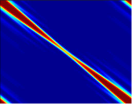
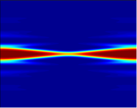
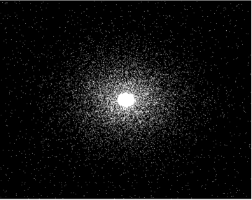
where S𝑆S is an index set of size at most k𝑘k and ASsubscript𝐴𝑆A_{S} denotes the selection of columns indexed by S𝑆S. In fact, we measure it more carefully by considering the local incoherence introduced in [15]. In contrast to the (isotropic) variable density sampling scheme introduced and analyzed in [15], our construction leads not unexpectedly to a set of highly directional random sampling schemes ΔMsubscriptΔ𝑀\Delta_{M}. It is though interesting to notice in which way the directionality appears, strongly concentrated along the angle bisectors.

We then prove that our novel sampling-reconstruction scheme is indeed asymptotically optimal (Theorem 3.5) in the sense of Subsection 1.4, which we will make a bit more precise later (Definition 3.1). To our knowledge this is the first optimality result for sampling-reconstruction schemes for Fourier data based on compressed sensing in the continuum setting. Besides the previously mentioned ingredients, one further key idea of our analysis is the approximation of the continuum situation by finite dimensional objects – in particular, at each level we consider a finite-dimensional shearlet system for reconstruction – in the spirit of, yet conceptionally different from the finite section method like approach of generalized sampling [4]. Moreover, our asymptotic analysis relies heavily on the multiscale structure of shearlets, though in contrast to the multiscale sparsity studied in [3], we also investigate sparsity patterns for cartoon-like functions with respect to directional parameters in the shearlet representation.

1.7. Outline

The paper is organized as follows. We start by introducing the main definitions and results for dualizable shearlets in Section 2. Section 3 is then devoted to introduce and discuss our novel sampling-reconstruction scheme, and state our optimality result. Its proof is presented in Section 4. Finally, numerical experiments comparing our scheme with other schemes are discussed in Section 5.

2. Dualizable Shearlets

Dualizable shearlets are one main ingredient in our sampling-reconstruction scheme, as discussed in the introduction. Hence this section shall serve as a review of the definition and main properties of dualizable shearlet frames. For further details we refer to [19].

As already indicated in the introduction, the composition of features (DS1)–(DS4) – which also distinguishes dualizable shearlet systems from “standard” shearlet systems (see [16]) – will enable us to derive an optimal sampling-reconstruction scheme.

2.1. Definition and Basic Notions

The construction consists of two steps. First, so-called shearlet-type wavelet systems are defined, which are unions of orthonormal bases, indexed by a shearing parameter. Second, a particular set of filters is used to cut out certain parts of those systems, to ensure directionality. Convolving both then leads to dualizable shearlet systems. In the spirit of the cone-based definition of standard shearlet systems (cf. [16]), these systems are composed of two parts: a system consisting of functions, for which the essential supports of their Fourier transforms are horizontally aligned, and a similar system associated with a vertical cone in Fourier domain – which is typically the rotated first system. We wish to mention that concerning the dualizable shearlet system we will only present the construction for the horizontal Fourier cone in detail, the vertically aligned system will be derived by switching the variables.

As our first step, aiming to construct a family of orthonormal bases for L2(2)superscript𝐿2superscript2L^{2}(\mathbb{R}^{2}) for each shearing direction, we choose two univariate functions φ1subscript𝜑1\varphi_{1} and ψ1subscript𝜓1\psi_{1} to satisfy the following definition. We wish to mention that as in the sequel the symbol less-than-or-similar-to\lesssim indicates the asymptotics for J𝐽J\to\infty.

Definition 2.1.

Let φ1,ψ1L2()subscript𝜑1subscript𝜓1superscript𝐿2\varphi_{1},\psi_{1}\in L^{2}(\mathbb{R}) be compactly supported and satisfy the support condition

δφ1=infξ[12,12]|φ^1(ξ)|>0,subscript𝛿subscript𝜑1subscriptinfimum𝜉1212subscript^𝜑1𝜉0\delta_{\varphi_{1}}=\inf_{\xi\in[-\frac{1}{2},\frac{1}{2}]}|\hat{\varphi}_{1}(\xi)|>0,

as well as, for some ρ(0,213)𝜌0213\rho\in(0,\frac{2}{13}), α6ρ+1𝛼6𝜌1\alpha\geq\frac{6}{\rho}+1, and β>α+1𝛽𝛼1\beta>\alpha+1, the decay conditions

|(ddξ)ψ^1(ξ)|min{1,|ξ|α}(1+|ξ|)βand|(ddξ)φ^1(ξ)|1(1+|ξ|)βfor =0,1.formulae-sequenceless-than-or-similar-tosuperscript𝑑𝑑𝜉subscript^𝜓1𝜉1superscript𝜉𝛼superscript1𝜉𝛽andformulae-sequenceless-than-or-similar-tosuperscript𝑑𝑑𝜉subscript^𝜑1𝜉1superscript1𝜉𝛽for 01\Bigl{|}\Bigl{(}\frac{d}{d\xi}\Bigr{)}^{\ell}\hat{\psi}_{1}(\xi)\Bigr{|}\lesssim\frac{\min\{1,|\xi|^{\alpha}\}}{(1+|\xi|)^{\beta}}\quad\mbox{and}\quad\Bigl{|}\Bigl{(}\frac{d}{d\xi}\Bigr{)}^{\ell}\hat{\varphi}_{1}(\xi)\Bigr{|}\lesssim\frac{1}{(1+|\xi|)^{\beta}}\quad\mbox{for }\ell=0,1.

We further assume that the system

{φ1(m):m}{2j/2ψ1(2jm):j0,m}\{\varphi_{1}(\cdot-m):m\in\mathbb{Z}\}\cup\{2^{j/2}\psi_{1}(2^{j}\cdot-m):j\geq 0,m\in\mathbb{Z}\}

forms an orthonormal basis for L2()superscript𝐿2L^{2}(\mathbb{R}). Then we refer to the pair (φ1,ψ1)subscript𝜑1subscript𝜓1(\varphi_{1},\psi_{1}) as (ρ,α,β)𝜌𝛼𝛽(\rho,\alpha,\beta)-admissible.

We remark that the condition to constitute an orthonormal basis can indeed be fulfilled by [8].

Let now (φ1,ψ1)subscript𝜑1subscript𝜓1(\varphi_{1},\psi_{1}) be (ρ,α,β)𝜌𝛼𝛽(\rho,\alpha,\beta)-admissible. Based on these univariate functions, for each x=(x1,x2)2𝑥subscript𝑥1subscript𝑥2superscript2x=(x_{1},x_{2})\in\mathbb{R}^{2}, we define

ψ0(x):=ψ1(x1)φ1(x2)andψp(x):=2(p1)/2ψ1(x1)ψ1(2p1x2)for p>0formulae-sequenceassignsuperscript𝜓0𝑥subscript𝜓1subscript𝑥1subscript𝜑1subscript𝑥2andassignsuperscript𝜓𝑝𝑥superscript2𝑝12subscript𝜓1subscript𝑥1subscript𝜓1superscript2𝑝1subscript𝑥2for 𝑝0\psi^{0}(x):=\psi_{1}(x_{1})\varphi_{1}(x_{2})\quad\mbox{and}\quad\psi^{p}(x):=2^{(p-1)/2}\psi_{1}(x_{1})\psi_{1}(2^{p-1}x_{2})\;\mbox{for }p>0 (3)

as well as

φ0(x):=φ1(x1)φ1(x2)andφp(x):=2(p1)/2φ1(x1)ψ1(2p1x2)for p>0.formulae-sequenceassignsuperscript𝜑0𝑥subscript𝜑1subscript𝑥1subscript𝜑1subscript𝑥2andassignsuperscript𝜑𝑝𝑥superscript2𝑝12subscript𝜑1subscript𝑥1subscript𝜓1superscript2𝑝1subscript𝑥2for 𝑝0\varphi^{0}(x):=\varphi_{1}(x_{1})\varphi_{1}(x_{2})\quad\mbox{and}\quad\varphi^{p}(x):=2^{(p-1)/2}\varphi_{1}(x_{1})\psi_{1}(2^{p-1}x_{2})\;\mbox{for }p>0. (4)

In this construction, the parameter p𝑝p enables a dyadic substructure in vertical direction. For a fixed integer j00subscript𝑗00j_{0}\geq 0, we now consider the system given by

{|det(Aj0)|1/2φp(Aj0Dpm),|det(Aj)|1/2ψp(AjDpm):jj0,p0},\{|\mathrm{det}(A_{j_{0}})|^{1/2}\varphi^{p}(A_{j_{0}}\cdot-D_{p}m),\>|\mathrm{det}(A_{j})|^{1/2}\psi^{p}(A_{j}\cdot-D_{p}m):j\geq j_{0},p\geq 0\},

where Dp=diag(1,2max{p1,0})subscript𝐷𝑝diag1superscript2𝑝10D_{p}=\mathrm{diag}(1,2^{-\max\{p-1,0\}}). By [19], this system forms an orthonormal basis for L2(2)superscript𝐿2superscript2L^{2}(\mathbb{R}^{2}).

We next recall that the shear parameter for a standard shearlet system should equal k2j/2𝑘superscript2𝑗2\frac{k}{2^{\lceil j/2\rceil}} for |k|2j/2𝑘superscript2𝑗2|k|\leq 2^{\lceil j/2\rceil}. Aiming to parameterize those quotients we define the injective map

s:{(j,q):j=0,q=0}{j:j0}×{q:|q|2j,q2+1}[1,1],s(j,q):=q2j,:𝑠formulae-sequenceconditional-set𝑗𝑞formulae-sequence𝑗0𝑞0conditional-set𝑗𝑗0conditional-set𝑞formulae-sequence𝑞superscript2𝑗𝑞2111assign𝑠𝑗𝑞𝑞superscript2𝑗s:\{(j,q):j=0,q=0\}\cup\{j:j\geq 0\}\times\{q:|q|\leq 2^{j},\,q\in 2\mathbb{Z}+1\}\to[-1,1],\,\,s(j,q):=\frac{q}{2^{j}},

as well as

𝕊={s(j,q)=0:j=0,q=0}{s(j,q):j0,|q|2j,q2+1}.𝕊conditional-set𝑠𝑗𝑞0formulae-sequence𝑗0𝑞0conditional-set𝑠𝑗𝑞formulae-sequence𝑗0formulae-sequence𝑞superscript2𝑗𝑞21\mathbb{S}=\{s(j,q)=0:j=0,q=0\}\cup\{s(j,q):j\geq 0,\,|q|\leq 2^{j},\,q\in 2\mathbb{Z}+1\}.

These preparations enable us to now defined shearlet-type wavelet systems.

Definition 2.2.

Let ρ(0,112)𝜌0112\rho\in(0,{\color[rgb]{0,0,0}\frac{1}{12}}), α6ρ+1𝛼6𝜌1\alpha\geq\frac{6}{\rho}+1, and β>α+1𝛽𝛼1\beta>\alpha+1. Let φ1,ψ1L2()subscript𝜑1subscript𝜓1superscript𝐿2\varphi_{1},\psi_{1}\in L^{2}(\mathbb{R}) with (φ1,ψ1)subscript𝜑1subscript𝜓1(\varphi_{1},\psi_{1}) being (ρ,α,β)𝜌𝛼𝛽(\rho,\alpha,\beta)-admissible, and let φp,ψpL2(2)superscript𝜑𝑝superscript𝜓𝑝superscript𝐿2superscript2\varphi^{p},\psi^{p}\in L^{2}(\mathbb{R}^{2}), p0𝑝0p\geq 0 satisfy (3) and (4). Further, set Dp:=diag(1,2dp)assignsubscript𝐷𝑝diag1superscript2subscript𝑑𝑝D_{p}:=\mathrm{diag}(1,2^{-d_{p}}) with dp:=max{p1,0}assignsubscript𝑑𝑝𝑝10d_{p}:=\max\{p-1,0\}. Then, for each shear parameter s:=s(j0/2,q0)𝕊assign𝑠𝑠subscript𝑗02subscript𝑞0𝕊s:=s(\lceil j_{0}/2\rceil,q_{0})\in\mathbb{S}, where j0subscript𝑗0j_{0} is the smallest nonnegative integer such that s=q02j0/2𝑠subscript𝑞0superscript2subscript𝑗02s=\frac{q_{0}}{2^{\lceil j_{0}/2\rceil}}, we define the shearlet-type wavelet system Ψs(φ1,ψ1)subscriptΨ𝑠subscript𝜑1subscript𝜓1\Psi_{s}(\varphi_{1},\psi_{1}) by

Ψs(φ1,ψ1):={φj0,s,m,p,ψj,s,m,p:jj0,m2,p0},assignsubscriptΨ𝑠subscript𝜑1subscript𝜓1conditional-setsubscript𝜑subscript𝑗0𝑠𝑚𝑝subscript𝜓𝑗𝑠𝑚𝑝formulae-sequence𝑗subscript𝑗0formulae-sequence𝑚superscript2𝑝0\Psi_{s}(\varphi_{1},\psi_{1}):=\{\varphi_{j_{0},s,m,p},\psi_{j,s,m,p}:j\geq j_{0},m\in\mathbb{Z}^{2},p\geq 0\},

where

φj,s,m,p:=|det(Aj)|1/2φp(AjSsDpm) and ψj,s,m,p:=|det(Aj)|1/2ψp(AjSsDpm).\varphi_{j,s,m,p}:=|\mathrm{det}(A_{j})|^{1/2}\varphi^{p}(A_{j}S_{s}\cdot-D_{p}m)\;\>\mbox{ and }\;\>\psi_{j,s,m,p}:=|\mathrm{det}(A_{j})|^{1/2}\psi^{p}(A_{j}S_{s}\cdot-D_{p}m).

The second step now consists in defining a filtering procedure. To be able to easier refer to properties of a generator and an associated filter, we introduce the following notion.

Definition 2.3.

Let ρ(0,213)𝜌0213\rho\in(0,\frac{2}{13}), α6ρ+1𝛼6𝜌1\alpha\geq\frac{6}{\rho}+1, and β>α+1𝛽𝛼1\beta>\alpha+1, and let gL2(2)𝑔superscript𝐿2superscript2g\in L^{2}(\mathbb{R}^{2}) be a compactly supported function satisfying the conic support condition

δg=infξΩg|g^(ξ)|>0,where Ωg={ξ2:|ξ2ξ1|<1,12<|ξ1|<1},formulae-sequencesubscript𝛿𝑔subscriptinfimum𝜉subscriptΩ𝑔^𝑔𝜉0where subscriptΩ𝑔conditional-set𝜉superscript2formulae-sequencesubscript𝜉2subscript𝜉1112subscript𝜉11\delta_{g}=\inf_{\xi\in\Omega_{g}}|\hat{g}(\xi)|>0,\quad\mbox{where }\Omega_{g}=\{\xi\in\mathbb{R}^{2}:|\tfrac{\xi_{2}}{\xi_{1}}|<1,\tfrac{1}{2}<|\xi_{1}|<1\Big{\}},

as well as the decay condition

|(ξ2)g^(ξ)|min{1,|ξ1|α}(1+|ξ1|)β(1+|ξ2|)βfor =0,1.formulae-sequenceless-than-or-similar-tosuperscriptsubscript𝜉2^𝑔𝜉1superscriptsubscript𝜉1𝛼superscript1subscript𝜉1𝛽superscript1subscript𝜉2𝛽for 01\Bigl{|}\Bigl{(}\frac{\partial}{\partial\xi_{2}}\Bigr{)}^{\ell}\hat{g}(\xi)\Bigr{|}\lesssim\frac{\min\{1,|\xi_{1}|^{\alpha}\}}{(1+|\xi_{1}|)^{\beta}(1+|\xi_{2}|)^{\beta}}\quad\mbox{for }\ell=0,1.

We then refer to the family of filters Gssubscript𝐺𝑠G_{s}, s=s(j0/2,q0)𝕊𝑠𝑠subscript𝑗02subscript𝑞0𝕊s=s(\lceil j_{0}/2\rceil,q_{0})\in\mathbb{S} defined by

G^0(ξ)=|φ^0(ξ)|2+j=0|g^(Aj1ξ)|2andG^s(ξ)=j=j0|g^(Aj1SsTξ)|2for s0formulae-sequencesubscript^𝐺0𝜉superscriptsuperscript^𝜑0𝜉2superscriptsubscript𝑗0superscript^𝑔subscriptsuperscript𝐴1𝑗𝜉2andformulae-sequencesubscript^𝐺𝑠𝜉superscriptsubscript𝑗subscript𝑗0superscript^𝑔subscriptsuperscript𝐴1𝑗subscriptsuperscript𝑆𝑇𝑠𝜉2for 𝑠0\hat{G}_{0}(\xi)=|\hat{\varphi}^{0}(\xi)|^{2}+\sum_{j=0}^{\infty}|\hat{g}(A^{-1}_{j}\xi)|^{2}\quad\mbox{and}\quad\hat{G}_{s}(\xi)=\sum_{j=j_{0}}^{\infty}|\hat{g}(A^{-1}_{j}S^{-T}_{s}\xi)|^{2}\quad\mbox{for }s\neq 0 (5)

as a family of (ρ,α,β;g)𝜌𝛼𝛽𝑔(\rho,\alpha,\beta;g)-filters.

Having introduced the two necessary ingredients, we can now formally define dualizable shearlet systems as follows. Notice that this definition will indeed require the systems derived by switching the variable in Ψs(φ1,ψ1)subscriptΨ𝑠subscript𝜑1subscript𝜓1\Psi_{s}(\varphi_{1},\psi_{1}), i.e., by R=(0110)𝑅0110R=\left(\begin{array}[]{cc}0&1\\ 1&0\\ \end{array}\right).

Definition 2.4 ([19]).

Let ρ(0,112)𝜌0112\rho\in(0,\frac{1}{12}), α6ρ+1𝛼6𝜌1\alpha\geq\frac{6}{\rho}+1, and β>α+1𝛽𝛼1\beta>\alpha+1. For any s𝕊𝑠𝕊s\in\mathbb{S}, let Ψs(φ1,ψ1)subscriptΨ𝑠subscript𝜑1subscript𝜓1\Psi_{s}(\varphi_{1},\psi_{1}) be a shearlet-type wavelet system, and let (Gs)s𝕊subscriptsubscript𝐺𝑠𝑠𝕊(G_{s})_{s\in\mathbb{S}} be a family of (ρ,α,β;g)𝜌𝛼𝛽𝑔(\rho,\alpha,\beta;g)-filters. Then the dualizable shearlet system 𝒮(φ1,ψ1;g)𝒮subscript𝜑1subscript𝜓1𝑔\mathcal{SH}(\varphi_{1},\psi_{1};g) is defined by

𝒮(φ1,ψ1;g)={ψλ:λΛs,s𝕊,=0,1}𝒮subscript𝜑1subscript𝜓1𝑔conditional-setsubscriptsuperscript𝜓𝜆formulae-sequence𝜆subscriptΛ𝑠formulae-sequence𝑠𝕊01\mathcal{SH}(\varphi_{1},\psi_{1};g)=\{\psi^{\ell}_{\lambda}:\lambda\in\Lambda_{s},s\in\mathbb{S},\ell=0,1\}

with index set

Λs={(j,s,m,p):j{1}{j0,j0+1,},m2,p0}for s=s(j0/2,q0),formulae-sequencesubscriptΛ𝑠conditional-set𝑗𝑠𝑚𝑝formulae-sequence𝑗1subscript𝑗0subscript𝑗01formulae-sequence𝑚superscript2𝑝0for 𝑠𝑠subscript𝑗02subscript𝑞0\Lambda_{s}=\{(j,s,m,p):j\in\{-1\}\cup\{j_{0},j_{0}+1,\ldots\},m\in\mathbb{Z}^{2},p\geq 0\}\quad\mbox{for }s=s(\lceil j_{0}/2\rceil,q_{0}),

where

ψλ0={Gsφj0,s,m,p:λ=(1,s,m,p)Λs,Gsψj,s,m,p:λ=(j,s,m,p)Λs,subscriptsuperscript𝜓0𝜆casessubscript𝐺𝑠subscript𝜑subscript𝑗0𝑠𝑚𝑝:𝜆1𝑠𝑚𝑝subscriptΛ𝑠subscript𝐺𝑠subscript𝜓𝑗𝑠𝑚𝑝:𝜆𝑗𝑠𝑚𝑝subscriptΛ𝑠\psi^{0}_{\lambda}=\left\{\begin{array}[]{rcl}G_{s}*\varphi_{j_{0},s,m,p}&:&\lambda=(-1,s,m,p)\in\Lambda_{s},\\ G_{s}*\psi_{j,s,m,p}&:&\lambda=(j,s,m,p)\in\Lambda_{s},\end{array}\right.

and ψλ1=ψλ0Rsubscriptsuperscript𝜓1𝜆subscriptsuperscript𝜓0𝜆𝑅\psi^{1}_{\lambda}=\psi^{0}_{\lambda}\circ R.

The following first two results from [19] state the announced properties of orthonormality (DS1) and compact support (DS2).

Proposition 2.5 ([19]).

For each s𝕊𝑠𝕊s\in\mathbb{S}, the shearlet-type wavelet system Ψs(φ1,ψ1)subscriptΨ𝑠subscript𝜑1subscript𝜓1\Psi_{s}(\varphi_{1},\psi_{1}) is an orthonormal basis for L2(2)superscript𝐿2superscript2L^{2}(\mathbb{R}^{2}).

Proposition 2.6 ([19]).

Each dualizable shearlet system is compactly supported.

The third already mentioned key property, i.e., (DS3), is the explicit form of one of the associated dual frames, made precise in the following statement.

Theorem 2.7 ([19]).

Let ρ(0,112)𝜌0112\rho\in(0,\frac{1}{12}), α6ρ+1𝛼6𝜌1\alpha\geq\frac{6}{\rho}+1, and β>α+1𝛽𝛼1\beta>\alpha+1. Let φ1,ψ1L2()subscript𝜑1subscript𝜓1superscript𝐿2\varphi_{1},\psi_{1}\in L^{2}(\mathbb{R}) with (φ1,ψ1)subscript𝜑1subscript𝜓1(\varphi_{1},\psi_{1}) being (ρ,α,β)𝜌𝛼𝛽(\rho,\alpha,\beta)-admissible, and let (Gs)s𝕊subscriptsubscript𝐺𝑠𝑠𝕊(G_{s})_{s\in\mathbb{S}} be a family of (ρ,α,β;g)𝜌𝛼𝛽𝑔(\rho,\alpha,\beta;g)-filters. Further, let 𝒮(φ1,ψ1;g)={ψλ:λΛs,s𝕊,=0,1}𝒮subscript𝜑1subscript𝜓1𝑔conditional-setsubscriptsuperscript𝜓𝜆formulae-sequence𝜆subscriptΛ𝑠formulae-sequence𝑠𝕊01\mathcal{SH}(\varphi_{1},\psi_{1};g)=\{\psi^{\ell}_{\lambda}:\lambda\in\Lambda_{s},s\in\mathbb{S},\ell=0,1\} be a dualizable shearlet system, which constitutes a frame for L2(2)superscript𝐿2superscript2L^{2}(\mathbb{R}^{2}). Then

𝒮~(φ1,ψ1;g)={ψ~λ:λΛs,s𝕊,=0,1}~𝒮subscript𝜑1subscript𝜓1𝑔conditional-setsubscriptsuperscript~𝜓𝜆formulae-sequence𝜆subscriptΛ𝑠formulae-sequence𝑠𝕊01\widetilde{\mathcal{SH}}(\varphi_{1},\psi_{1};g)=\{\tilde{\psi}^{\ell}_{\lambda}:\lambda\in\Lambda_{s},s\in\mathbb{S},\ell=0,1\}

is a dual frame for 𝒮(φ1,ψ1;g)𝒮subscript𝜑1subscript𝜓1𝑔\mathcal{SH}(\varphi_{1},\psi_{1};g), where, for λΛs𝜆subscriptΛ𝑠\lambda\in\Lambda_{s},

ψ~^λ0=ψ^λ0s𝕊|G^s|2+|G^sR|2andψ~λ1=ψ~λ0R.formulae-sequencesubscriptsuperscript^~𝜓0𝜆subscriptsuperscript^𝜓0𝜆subscriptsuperscript𝑠𝕊superscriptsubscript^𝐺superscript𝑠2superscriptsubscript^𝐺superscript𝑠𝑅2andsubscriptsuperscript~𝜓1𝜆subscriptsuperscript~𝜓0𝜆𝑅\hat{\tilde{\psi}}^{0}_{\lambda}=\frac{\hat{\psi}^{0}_{\lambda}}{\sum_{s^{\prime}\in\mathbb{S}}|\hat{G}_{s^{\prime}}|^{2}+|\hat{G}_{s^{\prime}}\circ{\color[rgb]{0,0,0}R}|^{2}}\quad\mbox{and}\quad\tilde{\psi}^{1}_{\lambda}=\tilde{\psi}^{0}_{\lambda}\circ{\color[rgb]{0,0,0}R}.

2.2. Sparse Approximation

We will next discuss the optimal sparse approximation properties dualizable shearlet systems satisfy. This anticipated behavior was before labeled as (DS4).

Since it is typically assumed that images are governed by anisotropic features, in particular, edges, a common model is the so-called class of cartoon-like functions. We start by formally introducing this class, which was first defined in [10].

Definition 2.8.

The set of cartoon-like functions 2(2)superscript2superscript2{\mathcal{E}}^{2}(\mathbb{R}^{2}) is defined by

2(2)={fL2(2):f=f0+f1χB},superscript2superscript2conditional-set𝑓superscript𝐿2superscript2𝑓subscript𝑓0subscript𝑓1subscript𝜒𝐵{\mathcal{E}}^{2}(\mathbb{R}^{2})=\{f\in L^{2}(\mathbb{R}^{2}):f=f_{0}+f_{1}\cdot\chi_{B}\},

where B[0,1]2𝐵superscript012B\subset[0,1]^{2} is a nonempty, simply connected set with C2superscript𝐶2C^{2}-boundary, B𝐵\partial B has bounded curvature, and fiC2(2)subscript𝑓𝑖superscript𝐶2superscript2f_{i}\in C^{2}(\mathbb{R}^{2}) satisfies suppfi[0,1]2suppsubscript𝑓𝑖superscript012\mathrm{supp}f_{i}\subseteq[0,1]^{2} and fiC21subscriptnormsubscript𝑓𝑖superscript𝐶21\|f_{i}\|_{C^{2}}\leq 1 for i=0,1𝑖01i=0,1.

In [10], Donoho proved a benchmark result in the sense of a lower bound for the achievable decay rate of the error of best N𝑁N-term approximation. One should mention that he in fact showed a more general result than the following statement; however this is what we require for our endeavour.

Theorem 2.9 ([10]).

Let (hi)iIL2(2)subscriptsubscript𝑖𝑖𝐼superscript𝐿2superscript2(h_{i})_{i\in I}\subseteq L^{2}(\mathbb{R}^{2}) be a frame for L2(2)superscript𝐿2superscript2L^{2}(\mathbb{R}^{2}). Then, for any f2(2)𝑓superscript2superscript2f\in{\mathcal{E}}^{2}(\mathbb{R}^{2}), the L2superscript𝐿2L^{2}-error of best N𝑁N-term approximation by fNsubscript𝑓𝑁f_{N} with respect to (hi)iIsubscriptsubscript𝑖𝑖𝐼(h_{i})_{i\in I} satisfies

ffN2N1as N.formulae-sequencegreater-than-or-equivalent-tosubscriptnorm𝑓subscript𝑓𝑁2superscript𝑁1as 𝑁\|f-f_{N}\|_{2}\gtrsim N^{-1}\qquad\text{as }N\rightarrow\infty.

Let us next assume that we are given a dualizable shearlet system

𝒮(φ1,ψ1;g)={ψλ:λΛs,s𝕊,=0,1}𝒮subscript𝜑1subscript𝜓1𝑔conditional-setsubscriptsuperscript𝜓𝜆formulae-sequence𝜆subscriptΛ𝑠formulae-sequence𝑠𝕊01\mathcal{SH}(\varphi_{1},\psi_{1};g)=\{\psi^{\ell}_{\lambda}:\lambda\in\Lambda_{s},s\in\mathbb{S},\ell=0,1\}

with associated dual frame

𝒮~(φ1,ψ1;g)={ψ~λ:λΛs,s𝕊,=0,1}~𝒮subscript𝜑1subscript𝜓1𝑔conditional-setsubscriptsuperscript~𝜓𝜆formulae-sequence𝜆subscriptΛ𝑠formulae-sequence𝑠𝕊01\widetilde{\mathcal{SH}}(\varphi_{1},\psi_{1};g)=\{\tilde{\psi}^{\ell}_{\lambda}:\lambda\in\Lambda_{s},s\in\mathbb{S},\ell=0,1\}

as defined in Theorem 2.7. Utilizing the more compact notation

Λ:={0,1}×s𝕊ΛsassignΛ01subscript𝑠𝕊subscriptΛ𝑠\Lambda:=\{0,1\}\times\bigcup_{s\in\mathbb{S}}\Lambda_{s}

for the index sets of those systems, we now consider N𝑁N-term approximations of f2(2)𝑓superscript2superscript2f\in{\mathcal{E}}^{2}(\mathbb{R}^{2}) of the form

fN=(,λ)ΛNf,ψλψ~λ,subscript𝑓𝑁subscript𝜆subscriptΛ𝑁𝑓subscriptsuperscript𝜓𝜆subscriptsuperscript~𝜓𝜆f_{N}=\sum_{(\ell,\lambda)\in\Lambda_{N}}\langle f,\psi^{\ell}_{\lambda}\rangle\tilde{\psi}^{\ell}_{\lambda},

where ΛNΛsubscriptΛ𝑁Λ\Lambda_{N}\subseteq\Lambda, #ΛN=N#subscriptΛ𝑁𝑁\#\Lambda_{N}=N. It might be surprising to consider expansions in terms of the dual frame, but in our case we have – and would like to use – knowledge on the decay of the frame coefficients (f,ψλ),λsubscript𝑓subscriptsuperscript𝜓𝜆𝜆(\langle f,\psi^{\ell}_{\lambda}\rangle)_{\ell,\lambda}.

The following result from [19] shows that the approximation rate of dualizable shearlets for cartoon-like functions can be arbitrarily close to the optimal rate as the smoothness of the generators is increased, i.e., as ρ0𝜌0\rho\to 0.

Theorem 2.10 ([19]).

Let ρ(0,112)𝜌0112\rho\in(0,\frac{1}{12}), α6ρ+1𝛼6𝜌1\alpha\geq\frac{6}{\rho}+1, and β>α+1𝛽𝛼1\beta>\alpha+1. Let φ1,ψ1L2()subscript𝜑1subscript𝜓1superscript𝐿2\varphi_{1},\psi_{1}\in L^{2}(\mathbb{R}) with (φ1,ψ1)subscript𝜑1subscript𝜓1(\varphi_{1},\psi_{1}) being (ρ,α,β)𝜌𝛼𝛽(\rho,\alpha,\beta)-admissible, and let (Gs)s𝕊subscriptsubscript𝐺𝑠𝑠𝕊(G_{s})_{s\in\mathbb{S}} be a family of (ρ,α,β;g)𝜌𝛼𝛽𝑔(\rho,\alpha,\beta;g)-filters. Further, let 𝒮(φ1,ψ1;g)={ψλ:λΛs,s𝕊,=0,1}𝒮subscript𝜑1subscript𝜓1𝑔conditional-setsubscriptsuperscript𝜓𝜆formulae-sequence𝜆subscriptΛ𝑠formulae-sequence𝑠𝕊01\mathcal{SH}(\varphi_{1},\psi_{1};g)=\{\psi^{\ell}_{\lambda}:\lambda\in\Lambda_{s},s\in\mathbb{S},\ell=0,1\} be a dualizable shearlet system, which constitutes a frame for L2(2)superscript𝐿2superscript2L^{2}(\mathbb{R}^{2}), and let f2(2)𝑓superscript2superscript2f\in\mathcal{E}^{2}(\mathbb{R}^{2}). Then

ffN2N1+12ρlog(N)as N,formulae-sequenceless-than-or-similar-tosubscriptnorm𝑓subscript𝑓𝑁2superscript𝑁112𝜌𝑁as 𝑁\|f-f_{N}\|_{2}\lesssim{\color[rgb]{0,0,0}N^{-1+12\rho}}\cdot\log(N)\qquad\text{as }N\rightarrow\infty,

where fN=(,λ)ΛNf,ψλψ~λsubscript𝑓𝑁subscript𝜆subscriptΛ𝑁𝑓subscriptsuperscript𝜓𝜆subscriptsuperscript~𝜓𝜆f_{N}=\sum_{(\ell,\lambda)\in\Lambda_{N}}\langle f,\psi^{\ell}_{\lambda}\rangle\tilde{\psi}^{\ell}_{\lambda} with ΛNΛsubscriptΛ𝑁Λ\Lambda_{N}\subseteq\Lambda, #ΛN=N#subscriptΛ𝑁𝑁\#\Lambda_{N}=N is the N𝑁N-term approximation using the N𝑁N largest coefficients (f,ψλ),λsubscript𝑓subscriptsuperscript𝜓𝜆𝜆(\langle f,\psi^{\ell}_{\lambda}\rangle)_{\ell,\lambda}.

Thus, dualizable shearlets do indeed satisfy (DS1)–(DS4).

3. Optimal Sampling-Reconstruction Scheme

We now turn to introducing our sampling-reconstruction scheme and stating the associated optimality result. But before, we first give a precise notion of optimality of sampling-reconstruction schemes, and – due to the technical difficulty of the construction and arguments – we will also provide some intuition on the construction of our scheme.

3.1. A Notion of Optimality

In Subsection 1.4, we already introduced a very general notion of optimality for general sampling-reconstruction schemes. We now make this precise in the setting we are considering.

We choose our model to be the model of cartoon-like functions 2(2)superscript2superscript2{\mathcal{E}}^{2}(\mathbb{R}^{2}) as defined in Definition 2.8) which, by Theorem 2.9, admits the following optimal decay rate of the best N𝑁N-term approximation:

ffN2N1 as N for all f2(2),less-than-or-similar-tosubscriptnorm𝑓subscript𝑓𝑁2superscript𝑁1 as 𝑁 for all 𝑓superscript2superscript2\|f-f_{N}\|_{2}\lesssim N^{-1}\mbox{ as }N\to\infty\mbox{ for all }f\in{\mathcal{E}}^{2}(\mathbb{R}^{2}),

where fN=λΛNcλψλsubscript𝑓𝑁subscript𝜆subscriptΛ𝑁subscript𝑐𝜆subscript𝜓𝜆f_{N}=\sum_{\lambda\in\Lambda_{N}}c_{\lambda}\psi_{\lambda} for some frame (ψλ)λΛL2(2)subscriptsubscript𝜓𝜆𝜆Λsuperscript𝐿2superscript2(\psi_{\lambda})_{\lambda\in\Lambda}\subseteq L^{2}(\mathbb{R}^{2}). Let now J𝐽J be a positive integer, and assume that we already constructed a set of sampling schemes

ΔJ2,J>0,with J#ΔJ strictly increasingformulae-sequencesubscriptΔ𝐽superscript2formulae-sequence𝐽0maps-towith 𝐽#subscriptΔ𝐽 strictly increasing\Delta_{J}\subseteq\mathbb{Z}^{2},J>0,\quad\mbox{with }J\mapsto\#\Delta_{J}\mbox{ strictly increasing} (6)

as well as an associated reconstruction scheme

=(2(2),Δ):2(2)×ΔL2(2),:superscript2superscript2Δsuperscript2superscript2Δsuperscript𝐿2superscript2\mathcal{R}=\mathcal{R}({\mathcal{E}}^{2}(\mathbb{R}^{2}),\Delta):{\mathcal{E}}^{2}(\mathbb{R}^{2})\times\Delta\to L^{2}(\mathbb{R}^{2}), (7)

where

Δ=J>0{ΔJ}.Δsubscript𝐽0subscriptΔ𝐽\Delta=\bigcup_{J>0}{\color[rgb]{0,0,0}\{\Delta_{J}\}}. (8)

We then introduce the following notion of optimality. We emphasize that we take an asymptotic viewpoint concerning optimality with J𝐽J being the parameter which provides the asymptotics. This is consistent with our continuum model in L2(2)superscript𝐿2superscript2L^{2}(\mathbb{R}^{2}) in the sense that we aim for an optimal behavior in this limit situation.

Definition 3.1.

A sampling-reconstruction scheme =(2(2),Δ)superscript2superscript2Δ\mathcal{R}=\mathcal{R}({\mathcal{E}}^{2}(\mathbb{R}^{2}),\Delta) is called asymptotically optimal, if, for all f2(2)𝑓superscript2superscript2f\in{\mathcal{E}}^{2}(\mathbb{R}^{2}),

f(f,ΔJ)2(#ΔJ)1as J.formulae-sequenceless-than-or-similar-tosubscriptnorm𝑓𝑓subscriptΔ𝐽2superscript#subscriptΔ𝐽1as 𝐽\|f-\mathcal{R}(f,\Delta_{J})\|_{2}\lesssim(\#\Delta_{J})^{-1}\quad\mbox{as }J\to\infty.

3.2. Intuition of Our Scheme

Before defining the sampling sets ΔJsubscriptΔ𝐽\Delta_{J}, J>0𝐽0J>0, and the reconstruction system similarly dependent on the scale J𝐽J, we will provide some first intuition for their choice. As already discussed in the introduction, we will choose a particular version of dualizable shearlet systems. In fact, for each limiting scale J𝐽J, we will choose a finite-dimensional version, which will turn out to be sufficient to derive an asymptotically optimal sampling-reconstruction scheme. A key ingredient will be the fact that those reconstruction systems will form orthonormal bases for each shear s𝑠s. The associated subset of the shearing parameters 𝕊𝕊\mathbb{S} associated with those finite-dimensional (dualizable) shearlet systems, will be chosen to be

𝕊J/2:={s(j,q)=0:j=0,q=0}{s(j/2,q):0jJ,|q|2j/2,q2+1},J>0.formulae-sequenceassignsubscript𝕊𝐽2conditional-set𝑠𝑗𝑞0formulae-sequence𝑗0𝑞0conditional-set𝑠𝑗2𝑞formulae-sequence0𝑗𝐽formulae-sequence𝑞superscript2𝑗2𝑞21𝐽0\mathbb{S}_{J/2}:=\{s(j,q)=0:j=0,q=0\}\cup\{s(\lceil j/2\rceil,q):0\leq j\leq J,\,|q|\leq 2^{\lceil j/2\rceil},\,q\in 2\mathbb{Z}+1\},\;J>0.

The sampling sets have then to be constructed such that the associated Fourier elements are maximally incoherent with the reconstruction system. To choose the sampling points in a suitable way requires analysis of the sparsity pattern of shearlet expansions of cartoon-like functions. Two sparsity pattern can be observed and need to be carefully handled:

  • Scale Dependence. The first sparsity pattern is the distribution of sparsity with respect to the scales j𝑗j. For this, we drive a strategy which is inspired by the variable density sampling strategy from [15], analyzing the local coherence terms of the shearlet elements and the elements of the Fourier basis. For each s𝕊J/2𝑠subscript𝕊𝐽2s\in\mathbb{S}_{J/2}, a suitable probability density function will then lead to a measurement matrix satisfying the Restricted Isometry Property with a sufficiently small restricted isometry constant with high probability. We remark that the orthogonality plays a prominent role in this analysis. Then, for each s𝑠s, we will reconstruct via 1subscript1\ell_{1} minimization, and finally patch the solutions together.

  • Shear Dependence. The second sparsity pattern we encounter is the distribution of sparsity with respect to the shear direction s𝑠s. To keep this under control, we will later slightly restrict the class of cartoon-like functions to ensure that the significant shearlet coefficients are almost equally distributed with respect to s𝑠s, which in a sense allows the patching of the solutions after the separate 1subscript1\ell_{1} minimizations.

As can be seen from this discussion, each ΔJsubscriptΔ𝐽\Delta_{J} needs to have a special substructure, namely, dependent on the shear s𝕊J/2𝑠subscript𝕊𝐽2s\in\mathbb{S}_{J/2}. In fact, the sampling sets will be constructed as a union of sampling sets ΔJ,ssubscriptΔ𝐽𝑠\Delta_{J,s}.

3.3. Sampling Systems

We first define the sampling sets – and with this the sampling systems – which we choose for (ΔJ)JsubscriptsubscriptΔ𝐽𝐽(\Delta_{J})_{J} in (6). Letting J>0𝐽0J>0, the complete sampling set has the form

ΩJ={(n1,n2)2:max(|n1|,|n2|)2J(1+ρ)}subscriptΩ𝐽conditional-setsubscript𝑛1subscript𝑛2superscript2less-than-or-similar-tosubscript𝑛1subscript𝑛2superscript2𝐽1𝜌\Omega_{J}=\{(n_{1},n_{2})\in\mathbb{Z}^{2}:\max(|n_{1}|,|n_{2}|)\lesssim 2^{J(1+\rho)}\}

with associated Fourier basis

ΦJ={en:=e2πi,n:n=(n1,n2)ΩJ}.subscriptΦ𝐽conditional-setassignsubscript𝑒𝑛superscript𝑒2𝜋𝑖𝑛𝑛subscript𝑛1subscript𝑛2subscriptΩ𝐽\Phi_{J}=\{e_{n}:=e^{2\pi i\langle\cdot,n\rangle}:n=(n_{1},n_{2})\in\Omega_{J}\}.

Let now j0subscript𝑗0j_{0} be an arbitrarily fixed scale. We then choose a sampling set ΔJ,ssubscriptΔ𝐽𝑠\Delta_{J,s} for each s=s(j0/2,q0)𝕊J/2𝑠𝑠subscript𝑗02subscript𝑞0subscript𝕊𝐽2s=s(\lceil j_{0}/2\rceil,q_{0})\in\mathbb{S}_{J/2} of size

mJ,s2Jj0223Jρ,similar-tosubscript𝑚𝐽𝑠superscript2𝐽subscript𝑗02superscript23𝐽𝜌m_{J,s}\sim 2^{\frac{J-j_{0}}{2}}{\color[rgb]{0,0,0}2^{3J\rho}},

i.e., dependent of s𝑠s. The mJ,ssubscript𝑚𝐽𝑠m_{J,s} sampling points ΔJ,ssubscriptΔ𝐽𝑠\Delta_{J,s} in ΩJsubscriptΩ𝐽\Omega_{J} are then chosen randomly according to the probability density function pJ,ssubscript𝑝𝐽𝑠p_{J,s} defined by

pJ,s(n)=csJ2(1+|n1|)(1+|n2sn1|)subscript𝑝𝐽𝑠𝑛subscript𝑐𝑠superscript𝐽21subscript𝑛11subscript𝑛2𝑠subscript𝑛1p_{J,s}(n)=\frac{c_{s}}{J^{2}(1+|n_{1}|)(1+|n_{2}-sn_{1}|)} (9)

over the discrete frequency domain ΩJsubscriptΩ𝐽\Omega_{J}, where the constant cssubscript𝑐𝑠c_{s} has obviously to be chosen so that nΩJps(n)=1subscript𝑛subscriptΩ𝐽subscript𝑝𝑠𝑛1\sum_{n\in\Omega_{J}}p_{s}(n)=1. Note that this condition implies that there exist some positive constants C1subscript𝐶1C_{1} and C2subscript𝐶2C_{2} such that C1<cs<C2subscript𝐶1subscript𝑐𝑠subscript𝐶2C_{1}<c_{s}<C_{2} for all s𝕊J/2𝑠subscript𝕊𝐽2s\in\mathbb{S}_{J/2}.

Thus, the random sampling sets (ΔJ)JsubscriptsubscriptΔ𝐽𝐽(\Delta_{J})_{J} employed in our sampling-reconstruction scheme are chosen as

ΔJ:=s𝕊J/2ΔJ,sassignsubscriptΔ𝐽subscript𝑠subscript𝕊𝐽2subscriptΔ𝐽𝑠\Delta_{J}:=\bigcup_{s\in\mathbb{S}_{J/2}}\Delta_{J,s} (10)

with associated sampling systems – as subsystems of ΦJsubscriptΦ𝐽\Phi_{J} – given by

{en:nΔJ,s,s𝕊J/2}.conditional-setsubscript𝑒𝑛formulae-sequence𝑛subscriptΔ𝐽𝑠𝑠subscript𝕊𝐽2\{e_{n}:n\in\Delta_{J,s},s\in\mathbb{S}_{J/2}\}.

Concerning the number of elements in each sampling set ΔJsubscriptΔ𝐽\Delta_{J}, we obtain the following result.

Lemma 3.2.

Let the sampling sets (ΔJ)JsubscriptsubscriptΔ𝐽𝐽(\Delta_{J})_{J} be defined as in (10). Then

#ΔJJ2J/2(1+6ρ).less-than-or-similar-to#subscriptΔ𝐽𝐽superscript2𝐽216𝜌\#\Delta_{J}\lesssim J\cdot 2^{J/2(1+{\color[rgb]{0,0,0}6\rho})}.
Proof.

We have

#ΔJ=s𝕊J/2mJ,sj0=0J2j0/22Jj0223JρJ2J/2(1+6ρ).#subscriptΔ𝐽subscript𝑠subscript𝕊𝐽2subscript𝑚𝐽𝑠less-than-or-similar-tosuperscriptsubscriptsubscript𝑗00𝐽superscript2subscript𝑗02superscript2𝐽subscript𝑗02superscript23𝐽𝜌less-than-or-similar-to𝐽superscript2𝐽216𝜌\#\Delta_{J}=\sum_{s\in\mathbb{S}_{J/2}}{\color[rgb]{0,0,0}m_{J,s}}\lesssim\sum_{j_{0}=0}^{J}2^{j_{0}/2}2^{\frac{J-j_{0}}{2}}{\color[rgb]{0,0,0}2^{3J\rho}}\lesssim J\cdot 2^{J/2(1+{\color[rgb]{0,0,0}6\rho})}.

This proves the claim. ∎

3.4. Reconstruction Systems

We continue by describing the representation systems we will employ for the reconstruction step. For this, we let ρ(0,112)𝜌0112\rho\in(0,{\color[rgb]{0,0,0}\frac{1}{12}}), α6ρ+1𝛼6𝜌1\alpha\geq\frac{6}{\rho}+1, and β>α+1𝛽𝛼1\beta>\alpha+1. Further, we choose φ1,ψ1L2()subscript𝜑1subscript𝜓1superscript𝐿2\varphi_{1},\psi_{1}\in L^{2}(\mathbb{R}) with (φ1,ψ1)subscript𝜑1subscript𝜓1(\varphi_{1},\psi_{1}) being (ρ,α,β)𝜌𝛼𝛽(\rho,\alpha,\beta)-admissible, and (Gs)s𝕊subscriptsubscript𝐺𝑠𝑠𝕊(G_{s})_{s\in\mathbb{S}} to form a family of (ρ,α,β;g)𝜌𝛼𝛽𝑔(\rho,\alpha,\beta;g)-filters. Let then 𝒮(φ1,ψ1;g)={ψλ:λΛs,s𝕊,=0,1}𝒮subscript𝜑1subscript𝜓1𝑔conditional-setsubscriptsuperscript𝜓𝜆formulae-sequence𝜆subscriptΛ𝑠formulae-sequence𝑠𝕊01\mathcal{SH}(\varphi_{1},\psi_{1};g)=\{\psi^{\ell}_{\lambda}:\lambda\in\Lambda_{s},s\in\mathbb{S},\ell=0,1\} be the associated dualizable shearlet system.

We next define finite-dimensional shearlet systems depending on J𝐽J and s𝑠s, which will serve as sparsifying systems for any fixed J𝐽J. For this, for each s=s(j0/2,q0)𝕊J/2𝑠𝑠subscript𝑗02subscript𝑞0subscript𝕊𝐽2s=s(\lceil j_{0}/2\rceil,q_{0})\in\mathbb{S}_{J/2}, we define the index set associated with those shearlets whose support basically intersects the support of the cartoon-like function f𝑓f, i.e.,

Λ~J,s={λ=(j,s,m,p)Λs:|supp(ψλ)[0,1]2|0,m2,pJρ2,j=j01,,J}.subscript~Λ𝐽𝑠conditional-set𝜆𝑗𝑠𝑚𝑝subscriptΛ𝑠formulae-sequencesuppsubscript𝜓𝜆superscript0120formulae-sequence𝑚superscript2formulae-sequence𝑝𝐽𝜌2𝑗subscript𝑗01𝐽\tilde{\Lambda}_{J,s}=\{\lambda=(j,s,m,p)\in\Lambda_{s}:|\operatorname*{supp}(\psi_{\lambda})\cap[0,1]^{2}|\neq 0,m\in\mathbb{Z}^{2},p\leq\frac{J\rho}{2},j=j_{0}-1,\dots,J\}. (11)

Recall that the support of f𝑓f is contained in [0,1]2superscript012[0,1]^{2}. As the observant reader will have noticed, we bounded the parameter p𝑝p, which will ensure that we now have “only” a finite-dimensional system to handle. Based on this index set, we next define a system ΨJ,ssubscriptΨ𝐽𝑠\Psi_{J,s}, with the property that GsΨJ,ssubscript𝐺𝑠subscriptΨ𝐽𝑠G_{s}*\Psi_{J,s} is a subsystem of 𝒮(φ1,ψ1;g)𝒮subscript𝜑1subscript𝜓1𝑔\mathcal{SH}(\varphi_{1},\psi_{1};g). The reason for this choice will become clear in the next subsection.

Definition 3.3.

Letting ρ(0,112)𝜌0112\rho\in(0,{\color[rgb]{0,0,0}\frac{1}{12}}), α6ρ+1𝛼6𝜌1\alpha\geq\frac{6}{\rho}+1, and β>α+1𝛽𝛼1\beta>\alpha+1. Further, we choose φ1,ψ1L2()subscript𝜑1subscript𝜓1superscript𝐿2\varphi_{1},\psi_{1}\in L^{2}(\mathbb{R}) with (φ1,ψ1)subscript𝜑1subscript𝜓1(\varphi_{1},\psi_{1}) being (ρ,α,β)𝜌𝛼𝛽(\rho,\alpha,\beta)-admissible, and (Gs)s𝕊subscriptsubscript𝐺𝑠𝑠𝕊(G_{s})_{s\in\mathbb{S}} to form a family of (ρ,α,β;g)𝜌𝛼𝛽𝑔(\rho,\alpha,\beta;g)-filters. Let also 𝒮(φ1,ψ1;g)={ψλ:λΛs,s𝕊,=0,1}𝒮subscript𝜑1subscript𝜓1𝑔conditional-setsubscriptsuperscript𝜓𝜆formulae-sequence𝜆subscriptΛ𝑠formulae-sequence𝑠𝕊01\mathcal{SH}(\varphi_{1},\psi_{1};g)=\{\psi^{\ell}_{\lambda}:\lambda\in\Lambda_{s},s\in\mathbb{S},\ell=0,1\} denote the associated dualizable shearlet system. For each J>0𝐽0J>0 and s𝕊J/2𝑠subscript𝕊𝐽2s\in\mathbb{S}_{J/2}, we then refer to

ΨJ,s={σλ:=1(ψ^λ/G^s):ψλ𝒮(φ1,ψ1;g),λΛ~J,s},subscriptΨ𝐽𝑠conditional-setassignsubscript𝜎𝜆superscript1subscript^𝜓𝜆subscript^𝐺𝑠formulae-sequencesubscript𝜓𝜆𝒮subscript𝜑1subscript𝜓1𝑔𝜆subscript~Λ𝐽𝑠\Psi_{J,s}=\{\sigma_{\lambda}:=\mathcal{F}^{-1}(\hat{\psi}_{\lambda}/\hat{G}_{s}):\psi_{\lambda}\in\mathcal{SH}(\varphi_{1},\psi_{1};g),\lambda\in\tilde{\Lambda}_{J,s}\},

where Λ~J,ssubscript~Λ𝐽𝑠\tilde{\Lambda}_{J,s} is defined as in (11), as the dualizable shearlet-reconstruction system for limiting scale J𝐽J and for shear direction s𝑠s.

We can immediately derive some basic properties of these systems.

Lemma 3.4.

Let ΨJ,ssubscriptΨ𝐽𝑠\Psi_{J,s} be a shearlet-reconstruction system for limiting scale J𝐽J and for shear direction s𝑠s. Then all elements in ΨJ,ssubscriptΨ𝐽𝑠\Psi_{J,s} are compactly supported, ΨJ,ssubscriptΨ𝐽𝑠\Psi_{J,s} forms an orthonormal basis for span(ΨJ,s)spansubscriptΨ𝐽𝑠\mbox{\rm span}(\Psi_{J,s}), and dim(span(ΨJ,s))2J/2(3+ρ)less-than-or-similar-todimensionspansubscriptΨ𝐽𝑠superscript2𝐽23𝜌\dim(\mbox{\rm span}(\Psi_{J,s}))\lesssim 2^{J/2(3+\rho)} as J𝐽J\to\infty

Proof.

Compact support immediately follows from Proposition 2.6. Moreover, Proposition 2.5 implies orthogonality, since ΨJ,sΨs(φ1,ψ1)subscriptΨ𝐽𝑠subscriptΨ𝑠subscript𝜑1subscript𝜓1\Psi_{J,s}\subset\Psi_{s}(\varphi_{1},\psi_{1}). The remaining claims follow from the observation that there exist about 232j2psuperscript232𝑗superscript2𝑝2^{\frac{3}{2}j}2^{p} elements σλΨJ,ssubscript𝜎𝜆subscriptΨ𝐽𝑠\sigma_{\lambda}\in\Psi_{J,s} for each parameter j𝑗j and p0𝑝0p\geq 0, hence the bounds jJ𝑗𝐽j\leq J and pJρ2𝑝𝐽𝜌2p\leq\frac{J\rho}{2} imply (ΨJ,s)2J2(3+ρ).less-than-or-similar-tosubscriptΨ𝐽𝑠superscript2𝐽23𝜌\sharp(\Psi_{J,s})\lesssim 2^{\frac{J}{2}(3+\rho)}.

3.5. Our Sampling-Reconstruction Scheme

We are now in a position to introduce the reconstruction scheme we choose for =(2(2),Δ)superscript2superscript2Δ\mathcal{R}=\mathcal{R}({\mathcal{E}}^{2}(\mathbb{R}^{2}),\Delta) in (7), with Δ=J>0{ΔJ}Δsubscript𝐽0subscriptΔ𝐽\Delta=\bigcup_{J>0}{\color[rgb]{0,0,0}\{\Delta_{J}\}} as just defined. To develop our scheme, for any f2(2)𝑓superscript2superscript2f\in{\mathcal{E}}^{2}(\mathbb{R}^{2}) and J>0𝐽0J>0, we need to define (f,ΔJ)𝑓subscriptΔ𝐽\mathcal{R}(f,\Delta_{J}). We remark that in fact we will define (f,ΔJ)𝑓subscriptΔ𝐽\mathcal{R}(f,\Delta_{J}) based on reconstructions from ΔJ,ssubscriptΔ𝐽𝑠\Delta_{J,s} for each s𝕊J/2𝑠subscript𝕊𝐽2s\in\mathbb{S}_{J/2}.

Now let f2(2)𝑓superscript2superscript2f\in{\mathcal{E}}^{2}(\mathbb{R}^{2}) and fix J𝐽J. Moreover, let s𝕊J/2𝑠subscript𝕊𝐽2s\in\mathbb{S}_{J/2} be arbitrarily fixed for now. We first expand some gL2(2)𝑔superscript𝐿2superscript2g\in L^{2}(\mathbb{R}^{2}) in terms of our chosen reconstruction system ΨJ,ssubscriptΨ𝐽𝑠\Psi_{J,s}. Since this system however only spans its closed linear hull and not L2(2)superscript𝐿2superscript2L^{2}(\mathbb{R}^{2}), we only obtain an expansion of the type

PΨJ,s(g)=λΛ~J,sg,σλσλ,subscript𝑃subscriptΨ𝐽𝑠𝑔subscript𝜆subscript~Λ𝐽𝑠𝑔subscript𝜎𝜆subscript𝜎𝜆P_{\Psi_{J,s}}(g)=\sum_{\lambda\in\tilde{\Lambda}_{J,s}}\langle g,\sigma_{\lambda}\rangle\sigma_{\lambda}, (12)

where PΨJ,ssubscript𝑃subscriptΨ𝐽𝑠P_{\Psi_{J,s}} denotes the orthogonal projection onto span(ΨJ,s)spansubscriptΨ𝐽𝑠\mbox{\rm span}(\Psi_{J,s}). Notice that the form of this expansion is only possible due to the fact that ΨJ,ssubscriptΨ𝐽𝑠\Psi_{J,s} forms an orthogonal basis, see Lemma 3.4. Next, we set g:=G¯sfassign𝑔subscript¯𝐺𝑠𝑓g:=\overline{G}_{s}*f and take the inner product of the previous equation with some element ensubscript𝑒𝑛e_{n}, n2𝑛superscript2n\in\mathbb{Z}^{2} of the Fourier basis, leading to

PΨJ,s(G¯sf),en=λΛ~J,sG¯sf,σλσλ,en.subscript𝑃subscriptΨ𝐽𝑠subscript¯𝐺𝑠𝑓subscript𝑒𝑛subscript𝜆subscript~Λ𝐽𝑠subscript¯𝐺𝑠𝑓subscript𝜎𝜆subscript𝜎𝜆subscript𝑒𝑛\langle P_{\Psi_{J,s}}(\overline{G}_{s}*f),e_{n}\rangle=\sum_{\lambda\in\tilde{\Lambda}_{J,s}}\langle\overline{G}_{s}*f,\sigma_{\lambda}\rangle\langle\sigma_{\lambda},e_{n}\rangle.

Recalling that by definition σλ:=1(ψ^λ/G^s)assignsubscript𝜎𝜆superscript1subscript^𝜓𝜆subscript^𝐺𝑠\sigma_{\lambda}:=\mathcal{F}^{-1}(\hat{\psi}_{\lambda}/\hat{G}_{s}) and using Plancherel twice, we obtain

PΨJ,s(G¯sf),en=λΛ~J,scλσλ,en,subscript𝑃subscriptΨ𝐽𝑠subscript¯𝐺𝑠𝑓subscript𝑒𝑛subscript𝜆subscript~Λ𝐽𝑠subscript𝑐𝜆subscript𝜎𝜆subscript𝑒𝑛\langle P_{\Psi_{J,s}}(\overline{G}_{s}*f),e_{n}\rangle=\sum_{\lambda\in\tilde{\Lambda}_{J,s}}c_{\lambda}\langle\sigma_{\lambda},e_{n}\rangle, (13)

where

cλ=G¯sf,σλ=f,ψλ.subscript𝑐𝜆subscript¯𝐺𝑠𝑓subscript𝜎𝜆𝑓subscript𝜓𝜆c_{\lambda}=\langle\overline{G}_{s}*f,\sigma_{\lambda}\rangle=\langle f,\psi_{\lambda}\rangle. (14)

We now claim that in applications, if we have access to f^(n)^𝑓𝑛\hat{f}(n), we also have access to PΨJ,s(G¯sf),ensubscript𝑃subscriptΨ𝐽𝑠subscript¯𝐺𝑠𝑓subscript𝑒𝑛\langle P_{\Psi_{J,s}}(\overline{G}_{s}*f),e_{n}\rangle. For this, first note that in computations we can only compute up to a particular scale. Hence the projection up to scale J𝐽J for J𝐽J large enough is no restriction. Second, the filter G¯ssubscript¯𝐺𝑠\overline{G}_{s} filters out the part of f𝑓f which corresponds to span(ΨJ,s)spansubscriptΨ𝐽𝑠\mbox{\rm span}(\Psi_{J,s}), hence can also be regarded as only causing a small, controllable error. Finally, by Plancherel, we have

G¯sf,en=G¯^s(n)f^(n),subscript¯𝐺𝑠𝑓subscript𝑒𝑛subscript^¯𝐺𝑠𝑛^𝑓𝑛\langle\overline{G}_{s}*f,e_{n}\rangle=\hat{\overline{G}}_{s}(n)\cdot\hat{f}(n),

which we indeed can compute knowing the action of the chosen filter G¯^s(n)subscript^¯𝐺𝑠𝑛\hat{\overline{G}}_{s}(n) as well as f^(n)^𝑓𝑛\hat{f}(n).

Applying now our choice for the sampling sets ΔJ,ssubscriptΔ𝐽𝑠\Delta_{J,s} from Subsection 3.3, the linear system of equations (13) becomes

PΨJ,s(G¯sf),en=λΛ~J,scλσλ,en,nΔJ,s.formulae-sequencesubscript𝑃subscriptΨ𝐽𝑠subscript¯𝐺𝑠𝑓subscript𝑒𝑛subscript𝜆subscript~Λ𝐽𝑠subscript𝑐𝜆subscript𝜎𝜆subscript𝑒𝑛𝑛subscriptΔ𝐽𝑠\langle P_{\Psi_{J,s}}(\overline{G}_{s}*f),e_{n}\rangle=\sum_{\lambda\in\tilde{\Lambda}_{J,s}}c_{\lambda}\langle\sigma_{\lambda},e_{n}\rangle,\quad n\in\Delta_{J,s}. (15)

Our reconstruction scheme solves this linear system of equations by exploiting the sparse approximation property of our chosen reconstruction system, i.e., we set

(f,ΔJ):=s𝕊J/2λΛ~J,sc^λψ~λ,assign𝑓subscriptΔ𝐽subscript𝑠subscript𝕊𝐽2subscript𝜆subscript~Λ𝐽𝑠subscript^𝑐𝜆subscript~𝜓𝜆\mathcal{R}(f,\Delta_{J}):=\sum_{s\in\mathbb{S}_{J/2}}\sum_{\lambda\in\tilde{\Lambda}_{J,s}}\hat{c}_{\lambda}\tilde{\psi}_{\lambda}, (16)

where

(c^λ)λΛ~J,s=argmin(c~λ)λΛ~J,s1 subject to (PΨJ,s(G¯sf),en=λΛ~J,sc~λσλ,en)nΔJ,s.subscriptsubscript^𝑐𝜆𝜆subscript~Λ𝐽𝑠argminsubscriptnormsubscriptsubscript~𝑐𝜆𝜆subscript~Λ𝐽𝑠1 subject to subscriptsubscript𝑃subscriptΨ𝐽𝑠subscript¯𝐺𝑠𝑓subscript𝑒𝑛subscript𝜆subscript~Λ𝐽𝑠subscript~𝑐𝜆subscript𝜎𝜆subscript𝑒𝑛𝑛subscriptΔ𝐽𝑠(\hat{c}_{\lambda})_{\lambda\in\tilde{\Lambda}_{J,s}}=\operatorname*{arg\,min}\|(\tilde{c}_{\lambda})_{\lambda\in\tilde{\Lambda}_{J,s}}\|_{1}\mbox{ subject to }\Bigg{(}\langle P_{\Psi_{J,s}}(\overline{G}_{s}*f),e_{n}\rangle=\sum_{\lambda\in\tilde{\Lambda}_{J,s}}\tilde{c}_{\lambda}\langle\sigma_{\lambda},e_{n}\rangle\Bigg{)}_{n\in\Delta_{J,s}}. (17)

In the sequel, instead of (15), we will often use the compact notation

𝐲𝐉,𝐬=AJ,s𝐜𝐉,𝐬subscript𝐲𝐉𝐬subscript𝐴𝐽𝑠subscript𝐜𝐉𝐬{\bf y_{J,s}}=A_{J,s}{\bf c_{J,s}} (18)

where 𝐲𝐉,𝐬=(PΨJ,s(G¯sf),en)nΔJ,ssubscript𝐲𝐉𝐬subscriptsubscript𝑃subscriptΨ𝐽𝑠subscript¯𝐺𝑠𝑓subscript𝑒𝑛𝑛subscriptΔ𝐽𝑠{\bf y_{J,s}}=(\langle P_{\Psi_{J,s}}(\overline{G}_{s}*f),e_{n}\rangle)_{n\in\Delta_{J,s}}, (AJ,s)n,λ=σλ,ensubscriptsubscript𝐴𝐽𝑠𝑛𝜆subscript𝜎𝜆subscript𝑒𝑛(A_{J,s})_{n,\lambda}=\langle\sigma_{\lambda},e_{n}\rangle, and 𝐜𝐉,𝐬=(cλ)λΛ~J,ssubscript𝐜𝐉𝐬subscriptsubscript𝑐𝜆𝜆subscript~Λ𝐽𝑠{\bf c_{J,s}}=(c_{\lambda})_{\lambda\in\tilde{\Lambda}_{J,s}}.

We finally wish to point out that in fact the very specific inner structure of the dualizable shearlet systems as well as of the associated dualizable shearlet-reconstruction systems only enabled this form of the linear system of equations. In fact, each of (DS1)–(DS3) have been exploited. The sparse approximation property (DS4) will then ensure that 1subscript1\ell_{1} minimization recovers an approximation with optimally small asymptotic error.

3.6. Main Result

We now have the sampling scheme ((8) and (10)) and the associated reconstruction scheme ((16) and (17)) at hand. The following theorem shows that our scheme is asymptotically optimal in the sense of Definition 3.1 for almost all cartoon-like functions. In fact, as announced in Subsection 3.2 we slightly restrict the set of cartoon-like functions to the set

~2(2)superscript~2superscript2\displaystyle\tilde{{\mathcal{E}}}^{2}(\mathbb{R}^{2}) :=assign\displaystyle:= {f2(2):fC2,r smooth with r[1/4,1) everywhere except for points\displaystyle\left\{f\in{\mathcal{E}}^{2}(\mathbb{R}^{2}):f\in C^{2,r}\mbox{ smooth with }r\in[1/4,1)\mbox{ everywhere except for points}\right.
lying on a C2 curve of non-vanishing curvature}.\displaystyle\hskip 5.69046pt\left.\mbox{lying on a }C^{2}\mbox{ curve of non-vanishing curvature}\right\}.

This condition ensures that the direction of the singularity curve of a cartoon-like function changes with a certain rate bounded from above, which leads to an almost equal distribution of the significant shearlet coefficients with respect to the shear s𝕊J/2𝑠subscript𝕊𝐽2s\in\mathbb{S}_{J/2} at a fixed scale J𝐽J. One instance of this can be seen in Proposition 4.4(ii).

We now have all ingredients to state the main result of this paper.

Theorem 3.5.

Letting ρ(0,213)𝜌0213\rho\in(0,\frac{2}{13}), α6ρ+1𝛼6𝜌1\alpha\geq\frac{6}{\rho}+1, and β>α+1𝛽𝛼1\beta>\alpha+1, we further choose φ1,ψ1L2()subscript𝜑1subscript𝜓1superscript𝐿2\varphi_{1},\psi_{1}\in L^{2}(\mathbb{R}) with (φ1,ψ1)subscript𝜑1subscript𝜓1(\varphi_{1},\psi_{1}) being (ρ,α,β)𝜌𝛼𝛽(\rho,\alpha,\beta)-admissible, and (Gs)s𝕊subscriptsubscript𝐺𝑠𝑠𝕊(G_{s})_{s\in\mathbb{S}} to form a family of (ρ,α,β;g)𝜌𝛼𝛽𝑔(\rho,\alpha,\beta;g)-filters. For each J>0𝐽0J>0 and s𝕊J/2𝑠subscript𝕊𝐽2s\in\mathbb{S}_{J/2}, let also ΨJ,ssubscriptΨ𝐽𝑠\Psi_{J,s} denote the associated dualizable shearlet-reconstruction system for limiting scale J𝐽J and for shear direction s𝑠s. Finally, let the sampling scheme ΔΔ\Delta be chosen as in (8) and (10), and let the reconstruction scheme \mathcal{R} be defined as in (16) and (17). Then there exists some universal constant C>0𝐶0C>0 (in particular, independent on ρ𝜌\rho), such that, for each f~2(2)𝑓superscript~2superscript2f\in\tilde{{\mathcal{E}}}^{2}(\mathbb{R}^{2}),

f(f,ΔJ)2(#ΔJ)1+ρCas J,formulae-sequenceless-than-or-similar-tosubscriptnorm𝑓𝑓subscriptΔ𝐽2superscript#subscriptΔ𝐽1𝜌𝐶as 𝐽\|f-\mathcal{R}(f,\Delta_{J})\|_{2}\lesssim(\#\Delta_{J})^{-1+\rho C}\quad\mbox{as }J\to\infty,

i.e., :~2(2)×ΔL2(2):superscript~2superscript2Δsuperscript𝐿2superscript2\mathcal{R}:\tilde{{\mathcal{E}}}^{2}(\mathbb{R}^{2})\times\Delta\to L^{2}(\mathbb{R}^{2}) is arbitrarily close to being asymptotically optimal.

Thus, our sampling-reconstruction scheme for reconstruction of the model class of cartoon-like functions from Fourier measurements is indeed asymptotically optimal, since ρ𝜌\rho can be chosen arbitrary small.

4. Proofs

This section is devoted to the proof of Theorem 3.5. We start with the overall structure and architecture of this proof, and then slowly delve into the details.

4.1. Architecture of the Proof of Theorem 3.5

As could already been predicted from the description of our sampling-reconstruction scheme in Subsection 3.5, also the proof relies heavily on the specific inner structure of dualizable shearlets, more precisely, of the dualizable shearlet-reconstruction systems for limiting scale J𝐽J and for shear direction s𝑠s. The proof will first estimate the error of the minimization procedure in (17) for each J𝐽J and s𝑠s, which will be subsequently combined mainly using the orthogonality stated in Lemma 3.4.

Given f~2(2)𝑓superscript~2superscript2f\in\tilde{{\mathcal{E}}}^{2}(\mathbb{R}^{2}), this splitting is performed by the estimate

f(f,ΔJ)2subscriptnorm𝑓𝑓subscriptΔ𝐽2\displaystyle\|f-\mathcal{R}(f,\Delta_{J})\|_{2} (19)
less-than-or-similar-to\displaystyle\lesssim j0=0Js{s(j/2,q)𝕊J/2:j=j0}𝐜𝐉,𝐬𝐜^𝐉,𝐬22+jJλΛj|f,ψλ|2+j=0JλΛj(Λj0)c|f,ψλ|2,superscriptsubscriptsubscript𝑗00𝐽subscript𝑠conditional-set𝑠superscript𝑗2superscript𝑞subscript𝕊𝐽2superscript𝑗subscript𝑗0subscriptsuperscriptnormsubscript𝐜𝐉𝐬subscript^𝐜𝐉𝐬22subscript𝑗𝐽subscript𝜆subscriptΛ𝑗superscript𝑓subscript𝜓𝜆2superscriptsubscript𝑗0𝐽subscript𝜆subscriptΛ𝑗superscriptsubscriptsuperscriptΛ0𝑗𝑐superscript𝑓subscript𝜓𝜆2\displaystyle\sum_{j_{0}=0}^{J}\sum_{s\in\{s(\lceil j^{{}^{\prime}}/2\rceil,q^{{}^{\prime}})\in\mathbb{S}_{J/2}:j^{{}^{\prime}}=j_{0}\}}\|{\bf c_{J,s}}-{\bf\hat{c}_{J,s}}\|^{2}_{2}+\sum_{j\geq J}\sum_{\lambda\in\Lambda_{j}}|\langle f,\psi_{\lambda}\rangle|^{2}+\sum_{j=0}^{J}\sum_{\lambda\in\Lambda_{j}\cap(\Lambda^{0}_{j})^{c}}|\langle f,\psi_{\lambda}\rangle|^{2},

where ΛjsubscriptΛ𝑗\Lambda_{j} is the set of all indices λ=(j,s,m,p)Λ𝜆𝑗𝑠𝑚𝑝Λ\lambda=(j,s,m,p)\in\Lambda with scale j𝑗j fixed and Λj0subscriptsuperscriptΛ0𝑗\Lambda^{0}_{j} is the subset of ΛjsubscriptΛ𝑗\Lambda_{j} where the oversampling parameters p𝑝p associated with Dpsubscript𝐷𝑝D_{p} are bounded by Jρ2𝐽𝜌2\frac{J\rho}{2}.

The first term in (19) will be handled by the following proposition.

Proposition 4.1.

We retain the same conditions and notations as in Theorem 3.5. Let 𝐜𝐉,𝐬:=(cλ)λΛ~J,s=(f,ψλ)λΛ~J,sassignsubscript𝐜𝐉𝐬subscriptsubscript𝑐𝜆𝜆subscript~Λ𝐽𝑠subscript𝑓subscript𝜓𝜆𝜆subscript~Λ𝐽𝑠{\bf c_{J,s}}:=(c_{\lambda})_{\lambda\in\tilde{\Lambda}_{J,s}}=(\langle f,\psi_{\lambda}\rangle)_{\lambda\in\tilde{\Lambda}_{J,s}} as in (14) and 𝐜^𝐉,𝐬:=(c^λ)λΛ~J,sassignsubscript^𝐜𝐉𝐬subscriptsubscript^𝑐𝜆𝜆subscript~Λ𝐽𝑠{\bf\hat{c}_{J,s}}:=(\hat{c}_{\lambda})_{\lambda\in\tilde{\Lambda}_{J,s}} be the solution of the 1subscript1\ell_{1} minimization problem (17). Then with probability at least 12J1superscript2𝐽1-2^{-J}, we have

𝐜𝐉,𝐬𝐜^𝐉,𝐬2σnJ,s(𝐜J,s)1nJ,sasJformulae-sequenceless-than-or-similar-tosubscriptnormsubscript𝐜𝐉𝐬subscript^𝐜𝐉𝐬2subscript𝜎subscript𝑛𝐽𝑠subscriptsubscript𝐜𝐽𝑠1subscript𝑛𝐽𝑠as𝐽\|{\bf c_{J,s}}-{\bf\hat{c}_{J,s}}\|_{2}\lesssim\frac{\sigma_{n_{J,s}}({\bf c}_{J,s})_{1}}{\sqrt{n_{J,s}}}\quad\text{as}\,\,J\rightarrow\infty

where

σnJ,s(𝐜𝐬)1:=inf{𝐜s𝐜~𝐬1:𝐜~𝐬0nJ,s}\sigma_{n_{J,s}}({\bf c_{s}})_{1}:=\inf\{\|{\bf c}_{s}-{\bf\tilde{c}_{s}}\|_{1}:\|{\bf\tilde{c}_{s}}\|_{0}\leq n_{J,s}\}

and nJ,sJ2Jj0222Jρsimilar-tosubscript𝑛𝐽𝑠𝐽superscript2𝐽subscript𝑗02superscript22𝐽𝜌n_{J,s}\sim J\cdot 2^{\frac{J-j_{0}}{2}}2^{{\color[rgb]{0,0,0}2J\rho}} for each s=s(j0/2,q0)𝕊J/2𝑠𝑠subscript𝑗02subscript𝑞0subscript𝕊𝐽2s=s(\lceil j_{0}/2\rceil,q_{0})\in\mathbb{S}_{J/2}.

One ingredient of the proof of this proposition, provided in Subsection 4.3.2, is a more or less classical result from compressed sensing. We state here the version presented in [15].

Theorem 4.2 ([15]).

Let Am×N𝐴superscript𝑚𝑁A\in\mathbb{C}^{m\times N} and xN𝑥superscript𝑁x\in\mathbb{C}^{N}. Suppose that y=Ax𝑦𝐴𝑥y=Ax where the restricted isometry constant of A𝐴A satisfies δ5s<13subscript𝛿5𝑠13\delta_{5s}<\frac{1}{3}. Then the solution to

minzNz1subject toAz=ysubscript𝑧superscript𝑁subscriptnorm𝑧1subject to𝐴𝑧𝑦\min_{z\in\mathbb{C}^{N}}\|z\|_{1}\quad\text{subject to}\quad Az=y

obeys

x^x2σs(x)1s.less-than-or-similar-tosubscriptnorm^𝑥𝑥2subscript𝜎𝑠subscript𝑥1𝑠\|\hat{x}-x\|_{2}\lesssim\frac{\sigma_{s}(x)_{1}}{\sqrt{s}}.

To apply this result, it needs to be shown that for the matrix A~J,ssubscript~𝐴𝐽𝑠\tilde{A}_{J,s} whose entries are given by

σλ,enmJ,spJ,s(n),nΔJ,s,λΛ~J,s,formulae-sequencesubscript𝜎𝜆subscript𝑒𝑛subscript𝑚𝐽𝑠subscript𝑝𝐽𝑠𝑛𝑛subscriptΔ𝐽𝑠𝜆subscript~Λ𝐽𝑠\frac{\langle\sigma_{\lambda},e_{n}\rangle}{\sqrt{m_{J,s}\cdot p_{J,s}(n)}},\quad n\in\Delta_{J,s},\lambda\in\tilde{\Lambda}_{J,s},

(compare the discussions in Subsections 1.1 and 1.3 as well as the definition of the 1subscript1\ell_{1} minimization problem (17)), its associated restricted isometry constant

δ^nJ,s:=max(S)nJ,sA~SA~SId2assignsubscript^𝛿subscript𝑛𝐽𝑠subscript𝑆subscript𝑛𝐽𝑠subscriptnormsubscriptsuperscript~𝐴𝑆subscript~𝐴𝑆Id2\hat{\delta}_{n_{J,s}}:=\max_{\sharp(S)\leq n_{J,s}}\|\tilde{A}^{*}_{S}\tilde{A}_{S}-\mathrm{Id}\|_{2}

can be made arbitrarily small. For this, a few ideas from [15] and [25] can be adapted and used. However, one main difficulty in our setting is to determine the required sampling size mJ,ssubscript𝑚𝐽𝑠m_{J,s} and the sparsity level nJ,ssubscript𝑛𝐽𝑠n_{J,s} for each shearing parameter s𝑠s by exploring sparsity patterns in the shearlet representation.

The second and third term in (19) require careful control of the decay of the shearlet coefficients. One key condition is that standard shearlets generated by Ajsubscript𝐴𝑗A_{j} and Sksubscript𝑆𝑘S_{k} are supported in Ss1Aj1[C,C]2subscriptsuperscript𝑆1𝑠subscriptsuperscript𝐴1𝑗superscript𝐶𝐶2S^{-1}_{s}A^{-1}_{j}[-C,C]^{2} for some C>0𝐶0C>0 with s=k2j/2𝑠𝑘superscript2𝑗2s=\frac{k}{2^{\lceil j/2\rceil}}. In this area, the C2superscript𝐶2C^{2} curvilinear singularity of a cartoon-like function is well approximated by its tangent. However, one can easily check that supp(ψλ)Ss1Aj01[C,C]2suppsubscript𝜓𝜆subscriptsuperscript𝑆1𝑠subscriptsuperscript𝐴1subscript𝑗0superscript𝐶𝐶2\mbox{supp}(\psi_{\lambda})\subset S^{-1}_{s}A^{-1}_{j_{0}}[-C,C]^{2}. In fact, supp(ψλ)suppsubscript𝜓𝜆\mbox{supp}(\psi_{\lambda}) is essentially the same as the support of standard shearlets considered in [18] for scale j=j0𝑗subscript𝑗0j=j_{0}. However, supp(ψλ)suppsubscript𝜓𝜆\mbox{supp}(\psi_{\lambda}) is much larger when jj0much-greater-than𝑗subscript𝑗0j\gg j_{0}. To resolve this issue, as already done in proofs in [19], we will approximate ψλsubscript𝜓𝜆\psi_{\lambda} by more suitable functions of smaller supports comparable to the size of the supports of standard shearlets with controllable error bound as follows:

For ψλ=Gsψj,s,m,psubscript𝜓𝜆subscript𝐺𝑠subscript𝜓𝑗𝑠𝑚𝑝\psi_{\lambda}=G_{s}*\psi_{j,s,m,p} with λ=(j,s,m,p)Λ,s=s(j0/2,q0)𝕊formulae-sequence𝜆𝑗𝑠𝑚𝑝Λ𝑠𝑠subscript𝑗02subscript𝑞0𝕊\lambda=(j,s,m,p)\in\Lambda,s=s(\lceil j_{0}/2\rceil,q_{0})\in\mathbb{S} and jj0𝑗subscript𝑗0j\geq j_{0}, define

ψ^λ(ξ)=j=max(j(1ρ),j0)|g^(AjSsξ)|2ψ^j,s,m,p(ξ).subscriptsuperscript^𝜓𝜆𝜉superscriptsubscriptsuperscript𝑗𝑗1𝜌subscript𝑗0superscript^𝑔subscriptsuperscript𝐴absentsuperscript𝑗subscriptsuperscript𝑆absent𝑠𝜉2subscript^𝜓𝑗𝑠𝑚𝑝𝜉\hat{\psi}^{\sharp}_{\lambda}(\xi)=\sum_{j^{{}^{\prime}}=\max(j(1-\rho),j_{0})}^{\infty}|\hat{g}(A^{-*}_{j^{{}^{\prime}}}S^{-*}_{s}\xi)|^{2}\hat{\psi}_{j,s,m,p}(\xi). (20)

Moreover, for ψλ𝒮(φ1,ψ1;g)subscript𝜓𝜆𝒮subscript𝜑1subscript𝜓1𝑔\psi_{\lambda}\in\mathcal{SH}(\varphi_{1},\psi_{1};g) of the form ψλ=Gsφj,s,m,psubscript𝜓𝜆subscript𝐺𝑠subscript𝜑𝑗𝑠𝑚𝑝\psi_{\lambda}=G_{s}*\varphi_{j,s,m,p}, we define ψλsubscriptsuperscript𝜓𝜆\psi^{\sharp}_{\lambda} as in (20) except for replacing ψ^j,s,m,psubscript^𝜓𝑗𝑠𝑚𝑝\hat{\psi}_{j,s,m,p} by φ^j,s,m,psubscript^𝜑𝑗𝑠𝑚𝑝\hat{\varphi}_{j,s,m,p}. Observe that for sufficiently small ρ>0𝜌0\rho>0, supp(ψλ)suppsubscriptsuperscript𝜓𝜆\mbox{supp}({\psi}^{\sharp}_{\lambda}) approximates the support of the original shearlet considered in [18] as follows.

Proposition 4.3 ([19]).

Let ψλL2(2)subscriptsuperscript𝜓𝜆superscript𝐿2superscript2\psi^{\sharp}_{\lambda}\in L^{2}(\mathbb{R}^{2}) as in (20). Then we have

supp(ψλ)Ss1Aj1([2jρC,2jρC]×[2j/2ρC,2j/2ρC]+Dpm)for someC>0.formulae-sequencesuppsubscriptsuperscript𝜓𝜆subscriptsuperscript𝑆1𝑠subscriptsuperscript𝐴1𝑗superscript2𝑗𝜌𝐶superscript2𝑗𝜌𝐶superscript2𝑗2𝜌𝐶superscript2𝑗2𝜌𝐶subscript𝐷𝑝𝑚for some𝐶0\operatorname*{supp}(\psi^{\sharp}_{\lambda})\subset S^{-1}_{s}A^{-1}_{j}\Bigl{(}[-2^{j\rho}C,2^{j\rho}C]\times[-2^{j/2\cdot\rho}C,2^{j/2\cdot\rho}C]+D_{p}m\Bigr{)}\quad\text{for some}\quad C>0.

Furthermore, we have

|f,(ψλψλ)|2jρα2pαf2forfL2(2).formulae-sequenceless-than-or-similar-to𝑓subscript𝜓𝜆subscriptsuperscript𝜓𝜆superscript2𝑗𝜌𝛼superscript2𝑝𝛼subscriptnorm𝑓2for𝑓superscript𝐿2superscript2|\langle f,(\psi_{\lambda}-\psi^{\sharp}_{\lambda})\rangle|\lesssim{\color[rgb]{0,0,0}2^{-j\rho\alpha}2^{-p\alpha}}\|f\|_{2}\quad\text{for}\quad f\in L^{2}(\mathbb{R}^{2}).

The decay estimates for the shearlet coefficients |f,ψλ|𝑓subscript𝜓𝜆|\langle f,\psi_{\lambda}\rangle| stated in the next result with (i) already being proven in [19] and (ii) in Subsection 4.3.1, will be the essential ingredients for controlling the first and second terms in (19).

Proposition 4.4 ([19]).

Assume that f𝑓f is a cartoon-like function with C2superscript𝐶2C^{2} discontinuity curve given by x1=E(x2)subscript𝑥1𝐸subscript𝑥2x_{1}=E(x_{2}). For ψλ𝒮(φ1,ψ1;g)subscript𝜓𝜆𝒮subscript𝜑1subscript𝜓1𝑔\psi_{\lambda}\in\mathcal{SH}(\varphi_{1},\psi_{1};g) with λ=(j,s,m,p)Λ𝜆𝑗𝑠𝑚𝑝Λ\lambda=(j,s,m,p)\in\Lambda and j0𝑗0j\geq 0, define ψλL2(2)subscriptsuperscript𝜓𝜆superscript𝐿2superscript2\psi^{\sharp}_{\lambda}\in L^{2}(\mathbb{R}^{2}) as in (20). Let x^2subscript^𝑥2\hat{x}_{2}\in\mathbb{R} so that (E(x^2),x^2)supp(ψλ)𝐸subscript^𝑥2subscript^𝑥2suppsubscriptsuperscript𝜓𝜆(E(\hat{x}_{2}),\hat{x}_{2})\in\mathrm{supp}(\psi^{\sharp}_{\lambda}) and s^=E(x^2)^𝑠superscript𝐸subscript^𝑥2\hat{s}=E^{{}^{\prime}}(\hat{x}_{2}). Also let kssubscript𝑘𝑠k_{s}\in\mathbb{Z} so that s=ks/2j/2𝑠subscript𝑘𝑠superscript2𝑗2s=k_{s}/2^{j/2}. Then for λ=(j,s,m,p)Λ𝜆𝑗𝑠𝑚𝑝Λ\lambda=(j,s,m,p)\in\Lambda with j0𝑗0j\geq 0, the following hold.

  • (i)

    If |s^|3^𝑠3|\hat{s}|\leq 3, then

    |f,ψλ|min(234j,234j23ρj|ks+2j/2s^|3).|\langle f,\psi_{\lambda}\rangle|\lesssim\min\Bigl{(}2^{-\frac{3}{4}j},\frac{2^{-\frac{3}{4}j}2^{3\rho j}}{|k_{s}+2^{j/2}\hat{s}|^{3}}\Bigl{)}.
  • (ii)

    If hL2(2)superscript𝐿2superscript2h\in L^{2}(\mathbb{R}^{2}) is C2,rsuperscript𝐶2𝑟C^{2,r} smooth in supp(ψλ)suppsubscriptsuperscript𝜓𝜆\operatorname*{supp}(\psi^{\sharp}_{\lambda}) with hC2,r(supp(ψλ))Csubscriptnormsuperscript𝐶2𝑟suppsubscriptsuperscript𝜓𝜆𝐶\|h\|_{C^{2,r}(\operatorname*{supp}(\psi^{\sharp}_{\lambda}))}\leq C and r[1/4,1)𝑟141r\in[1/4,1) for some C>0𝐶0C>0, then

    |h,ψλ|2p/22(34ρ)j.less-than-or-similar-tosubscript𝜓𝜆superscript2𝑝2superscript234𝜌𝑗|\langle h,\psi_{\lambda}\rangle|\lesssim 2^{p/2}2^{-(3-4\rho)j}.

Comparing with the standard shearlets considered in [18], our dualizable shearlet system 𝒮(φ1,ψ1;g)𝒮subscript𝜑1subscript𝜓1𝑔\mathcal{SH}(\varphi_{1},\psi_{1};g) has an additional parameter p𝑝p associated with the oversampling matrix Dpsubscript𝐷𝑝D_{p}. In addition to decay estimates in Proposition 4.4, we therefore need the decay of the shearlet coefficients with respect to p𝑝p. The following proposition shows how shearlet coefficients f,ψλ𝑓subscript𝜓𝜆\langle f,\psi_{\lambda}\rangle with this additional parameter p𝑝p can be controlled, which will be a crucial ingredient for controlling the third term in (19).

Proposition 4.5 ([19]).

For fL2(2)𝑓superscript𝐿2superscript2f\in L^{2}(\mathbb{R}^{2}), we have

|f,ψλ|2α2pf2for all λ=(j,s,p,m)Λ.formulae-sequenceless-than-or-similar-to𝑓subscript𝜓𝜆superscript2𝛼2𝑝subscriptnorm𝑓2for all 𝜆𝑗𝑠𝑝𝑚Λ|\langle f,\psi_{\lambda}\rangle|\lesssim 2^{-\frac{\alpha}{2}p}\cdot\|f\|_{2}\quad\text{for all }\lambda=(j,s,p,m)\in\Lambda.

Let us finally mention that in the subsequent proofs, without loss of generality, we will only consider shearlet elements ψλ0𝒮(φ1,ψ1;g)subscriptsuperscript𝜓0𝜆𝒮subscript𝜑1subscript𝜓1𝑔\psi^{0}_{\lambda}\in\mathcal{SH}(\varphi_{1},\psi_{1};g) associated with one frequency cone. Since the elements ψλ1subscriptsuperscript𝜓1𝜆\psi^{1}_{\lambda} are given by switching the variables with R𝑅R, they can be dealt with similarly. Hence, for the sake of brevity, we will often omit the superscript “0”, i.e., we write

ψλ:=ψλ0andψ~λ:=ψ~λ0.formulae-sequenceassignsubscript𝜓𝜆subscriptsuperscript𝜓0𝜆andassignsubscript~𝜓𝜆subscriptsuperscript~𝜓0𝜆\psi_{\lambda}:=\psi^{0}_{\lambda}\quad\mbox{and}\quad\tilde{\psi}_{\lambda}:=\tilde{\psi}^{0}_{\lambda}.

Moreover, for technical reasons, again without loss of generality, we now rescale each element σλΨJ,ssubscript𝜎𝜆subscriptΨ𝐽𝑠\sigma_{\lambda}\in\Psi_{J,s} so that

supp(σλ)[0,1]2,for all λΛ~J,s.formulae-sequencesuppsubscript𝜎𝜆superscript012for all 𝜆subscript~Λ𝐽𝑠\operatorname*{supp}(\sigma_{\lambda})\subset[0,1]^{2},\quad\mbox{for all }\lambda\in\tilde{\Lambda}_{J,s}.

4.2. Useful Lemmata from [25]

For the convenience of the reader, we state two lemmata both from [25], which will be required for the proof of Proposition 4.1.

Lemma 4.6 ([25]).

Assume that X=(X)=1m𝑋superscriptsubscriptsubscript𝑋1𝑚X=(X_{\ell})_{\ell=1}^{m} is a sequence of independent random vectors in Nsuperscript𝑁\mathbb{C}^{N} with XKsubscriptnormsubscript𝑋𝐾\|X_{\ell}\|_{\infty}\leq K for =1,,m1𝑚\ell=1,\dots,m. Then, for 1p<1𝑝1\leq p<\infty and nm𝑛𝑚n\leq m,

(𝔼|=1m(XiX𝔼XX)|np)1p2(𝔼|=1mϵXX|np)1p,superscript𝔼subscriptsuperscriptnormsuperscriptsubscript1𝑚subscriptsuperscript𝑋𝑖subscript𝑋𝔼subscriptsuperscript𝑋subscript𝑋𝑝𝑛1𝑝2superscript𝔼superscriptsubscriptnormsuperscriptsubscript1𝑚subscriptitalic-ϵsubscriptsuperscript𝑋subscript𝑋𝑛𝑝1𝑝\Bigl{(}\mathbb{E}{\left|\kern-1.07639pt\left|\kern-1.07639pt\left|\sum_{\ell=1}^{m}(X^{*}_{i}X_{\ell}-\mathbb{E}X^{*}_{\ell}X_{\ell})\right|\kern-1.07639pt\right|\kern-1.07639pt\right|}^{p}_{n}\Bigr{)}^{\frac{1}{p}}\leq 2\Bigl{(}\mathbb{E}{\left|\kern-1.07639pt\left|\kern-1.07639pt\left|\sum_{\ell=1}^{m}\epsilon_{\ell}X^{*}_{\ell}X_{\ell}\right|\kern-1.07639pt\right|\kern-1.07639pt\right|}_{n}^{p}\Bigr{)}^{\frac{1}{p}},

where ϵ=(ϵ)=1mitalic-ϵsuperscriptsubscriptsubscriptitalic-ϵ1𝑚\epsilon=(\epsilon_{\ell})_{\ell=1}^{m} is a Rademacher sequence independent of X𝑋X. Furthermore, for p2𝑝2p\geq 2,

(𝔼|=1mϵXX|np)1pCη1pKpnlog(100n)log(4N)log(10m)|=1mXX|n,superscript𝔼superscriptsubscriptnormsuperscriptsubscript1𝑚subscriptitalic-ϵsubscript𝑋subscriptsuperscript𝑋𝑛𝑝1𝑝𝐶superscript𝜂1𝑝𝐾𝑝𝑛100𝑛4𝑁10𝑚subscriptnormsuperscriptsubscript1𝑚subscript𝑋subscriptsuperscript𝑋𝑛\Bigl{(}\mathbb{E}{\left|\kern-1.07639pt\left|\kern-1.07639pt\left|\sum_{\ell=1}^{m}\epsilon_{\ell}X_{\ell}X^{*}_{\ell}\right|\kern-1.07639pt\right|\kern-1.07639pt\right|}_{n}^{p}\Bigr{)}^{\frac{1}{p}}\leq C{\eta}^{\frac{1}{p}}K\sqrt{p}\sqrt{n}\log(100n)\sqrt{\log(4N)\log(10m)}\sqrt{{\left|\kern-1.07639pt\left|\kern-1.07639pt\left|\sum_{\ell=1}^{m}X_{\ell}X^{*}_{\ell}\right|\kern-1.07639pt\right|\kern-1.07639pt\right|}_{n}},

where C𝐶C and η𝜂\eta are some positive constants and η<7𝜂7\eta<7.

Lemma 4.7.

[25]  Suppose that Z𝑍Z is a random variable satisfying

(𝔼|Z|p)1pC1C21pp1rfor allpp0formulae-sequencesuperscript𝔼superscript𝑍𝑝1𝑝subscript𝐶1superscriptsubscript𝐶21𝑝superscript𝑝1𝑟for all𝑝subscript𝑝0(\mathbb{E}|Z|^{p})^{\frac{1}{p}}\leq C_{1}C_{2}^{\frac{1}{p}}p^{\frac{1}{r}}\quad\text{for all}\,\,p\geq p_{0}

for some C1subscript𝐶1C_{1}, C2subscript𝐶2C_{2}, r𝑟r, p0>0subscript𝑝00p_{0}>0. Then

(|Z|e1rC1u)C2eur/rfor allup01r.formulae-sequence𝑍superscript𝑒1𝑟subscript𝐶1𝑢subscript𝐶2superscript𝑒superscript𝑢𝑟𝑟for all𝑢superscriptsubscript𝑝01𝑟\mathbb{P}(|Z|\geq e^{\frac{1}{r}}C_{1}u)\leq C_{2}e^{-u^{r}/r}\quad\text{for all}\,\,u\geq p_{0}^{\frac{1}{r}}.

4.3. Proof of Preparatory Results

4.3.1. Proof of Proposition 4.4(ii)

First notice that, by the error estimate in Proposition 4.3, it suffices to show that

|h,ψλ|2p/22(34ρ)jfor λ=(j,0,0,p)Λ.formulae-sequenceless-than-or-similar-tosubscriptsuperscript𝜓𝜆superscript2𝑝2superscript234𝜌𝑗for 𝜆𝑗00𝑝Λ|\langle h,\psi^{\sharp}_{\lambda}\rangle|\lesssim 2^{p/2}2^{-(3-4\rho)j}\quad\mbox{for }\lambda=(j,0,0,p)\in\Lambda. (21)

Hence, let λ=(j,0,0,p)𝜆𝑗00𝑝\lambda=(j,0,0,p). Again by Proposition 4.3, there exists some L>0𝐿0L>0 with

supp(ψλ)[2j+ρjL,2j+ρjL]×[2j/2+ρj/2L,2j/2+ρj/2L].suppsubscriptsuperscript𝜓𝜆superscript2𝑗𝜌𝑗𝐿superscript2𝑗𝜌𝑗𝐿superscript2𝑗2𝜌𝑗2𝐿superscript2𝑗2𝜌𝑗2𝐿\operatorname*{supp}(\psi^{\sharp}_{\lambda})\subset[-2^{-j+\rho j}L,2^{-j+\rho j}L]\times[-2^{-j/2+\rho j/2}L,2^{-j/2+\rho j/2}L]. (22)

Further, by construction, ψλsubscriptsuperscript𝜓𝜆\psi^{\sharp}_{\lambda} satisfies the vanishing moment condition

x1ψλ(x1,x2)𝑑x1=0for=0,1,2andψλ234j2p/2.formulae-sequencesubscriptsuperscriptsubscript𝑥1subscriptsuperscript𝜓𝜆subscript𝑥1subscript𝑥2differential-dsubscript𝑥10formulae-sequencefor012andless-than-or-similar-tosubscriptnormsubscriptsuperscript𝜓𝜆superscript234𝑗superscript2𝑝2\int_{\mathbb{R}}x_{1}^{\ell}\cdot\psi^{\sharp}_{\lambda}(x_{1},x_{2})dx_{1}=0\quad\text{for}\,\,\ell=0,1,2\quad\text{and}\quad\|\psi^{\sharp}_{\lambda}\|_{\infty}\lesssim 2^{\frac{3}{4}j}2^{p/2}.

Now let hC2,r(2)superscript𝐶2𝑟superscript2h\in C^{2,r}(\mathbb{R}^{2}), and observe that we may write hh as

h(x1,x2)==02(1!)(x1)h(0,x2)x1+R(x1,x2)x19/4for each(x1,x2)supp(ψλ)formulae-sequencesubscript𝑥1subscript𝑥2superscriptsubscript021superscriptsubscript𝑥10subscript𝑥2superscriptsubscript𝑥1𝑅subscript𝑥1subscript𝑥2superscriptsubscript𝑥194for eachsubscript𝑥1subscript𝑥2suppsubscriptsuperscript𝜓𝜆h(x_{1},x_{2})=\sum_{\ell=0}^{2}\Bigl{(}\frac{1}{\ell!}\Bigr{)}\Bigl{(}\frac{\partial}{\partial x_{1}}\Bigr{)}^{\ell}h(0,x_{2}){x_{1}}^{\ell}+R(x_{1},x_{2})x_{1}^{9/4}\quad\text{for each}\,\,(x_{1},x_{2})\in\operatorname*{supp}(\psi^{\sharp}_{\lambda}) (23)

for some bounded function g𝑔{\color[rgb]{0,0,0}g} with gCsubscriptnorm𝑔𝐶\|{\color[rgb]{0,0,0}g}\|_{\infty}\leq C for some C>0𝐶0C>0. Finally, by (22)–(23), we obtain

|h,ψλ|subscriptsuperscript𝜓𝜆\displaystyle|\langle h,\psi^{\sharp}_{\lambda}\rangle| less-than-or-similar-to\displaystyle\lesssim gψλ2j/2(1ρ)L2j/2(1ρ)L2j(1ρ)L2j(1ρ)L|x1|9/4𝑑x1𝑑x2subscriptnorm𝑔subscriptnormsubscriptsuperscript𝜓𝜆superscriptsubscriptsuperscript2𝑗21𝜌𝐿superscript2𝑗21𝜌𝐿superscriptsubscriptsuperscript2𝑗1𝜌𝐿superscript2𝑗1𝜌𝐿superscriptsubscript𝑥194differential-dsubscript𝑥1differential-dsubscript𝑥2\displaystyle\|{\color[rgb]{0,0,0}g}\|_{\infty}\|\psi^{\sharp}_{\lambda}\|_{\infty}\int_{-2^{-j/2(1-\rho)}L}^{2^{-j/2(1-\rho)}L}\int_{-2^{-j(1-\rho)}L}^{2^{-j(1-\rho)}L}|x_{1}|^{9/4}dx_{1}dx_{2}
less-than-or-similar-to\displaystyle\lesssim 234j2p/22j/2(1ρ)2j134(1ρ)2p22(34ρ)jsuperscript234𝑗superscript2𝑝2superscript2𝑗21𝜌superscript2𝑗1341𝜌superscript2𝑝2superscript234𝜌𝑗\displaystyle 2^{\frac{3}{4}j}2^{p/2}2^{-j/2(1-\rho)}2^{-j\frac{13}{4}(1-\rho)}\leq 2^{\frac{p}{2}}2^{-(3-4\rho)j}

This proves (21), and hence the claim. ∎

4.3.2. Proof of Proposition 4.1

The main part of this proof will be to show that Proposition 4.2 can be applied in a particular way. For this, let s=s(j0/2,q0)𝕊J/2𝑠𝑠subscript𝑗02subscript𝑞0subscript𝕊𝐽2s=s(\lceil j_{0}/2\rceil,q_{0})\in\mathbb{S}_{J/2}, and set ΔJ,s=:{t1,,tmJ,s}\Delta_{J,s}=:\{t_{1},\ldots,t_{m_{J,s}}\}. Moreover, let A𝐴A be the matrix defined by

(A~J,s)i,λ:=σ^λ(ti)mJ,spJ,s(ti)forλΛ~J,sandi=1,,mJ,s,formulae-sequenceformulae-sequenceassignsubscriptsubscript~𝐴𝐽𝑠𝑖𝜆subscript^𝜎𝜆subscript𝑡𝑖subscript𝑚𝐽𝑠subscript𝑝𝐽𝑠subscript𝑡𝑖for𝜆subscript~Λ𝐽𝑠and𝑖1subscript𝑚𝐽𝑠(\tilde{A}_{J,s})_{i,\lambda}:=\frac{\hat{\sigma}_{\lambda}(t_{i})}{\sqrt{m_{J,s}\cdot p_{J,s}(t_{i})}}\quad\text{for}\,\,\lambda\in\tilde{\Lambda}_{J,s}\,\,\text{and}\,\,i=1,\ldots,m_{J,s},

where σ^λ(ti)=σλ,etisubscript^𝜎𝜆subscript𝑡𝑖subscript𝜎𝜆subscript𝑒subscript𝑡𝑖\hat{\sigma}_{\lambda}(t_{i})=\langle\sigma_{\lambda},e_{t_{i}}\rangle and the tisubscript𝑡𝑖t_{i}’s are drawn from the probability density function pJ,ssubscript𝑝𝐽𝑠p_{J,s}. One should compare this choice with (18), seeing that it deviates from A𝐴A by (mJ,spJ,s(ti))1/2superscriptsubscript𝑚𝐽𝑠subscript𝑝𝐽𝑠subscript𝑡𝑖12(m_{J,s}\cdot p_{J,s}(t_{i}))^{1/2}. Further, let S𝑆S be any set of the column indices of A~~𝐴\tilde{A} with (S)nJ,s𝑆subscript𝑛𝐽𝑠\sharp(S)\leq n_{J,s}, and A~Ssubscript~𝐴𝑆\tilde{A}_{S} be the column submatrix of A~~𝐴\tilde{A} consisting of columns indexed by S𝑆S. Observe that (BST)STsubscriptsuperscriptsubscriptsuperscript𝐵𝑇𝑆𝑇𝑆(B^{T}_{S})^{T}_{S} is the submatrix of B𝐵B consisting of columns and rows indexed by S𝑆S, when B𝐵B is a square matrix.

We will now prove that the restricted isometry constant of A~~𝐴\tilde{A} given by

δ^nJ,s:=max(S)nJ,sA~SA~SId2assignsubscript^𝛿subscript𝑛𝐽𝑠subscript𝑆subscript𝑛𝐽𝑠subscriptnormsubscriptsuperscript~𝐴𝑆subscript~𝐴𝑆Id2\hat{\delta}_{n_{J,s}}:=\max_{\sharp(S)\leq n_{J,s}}\|\tilde{A}^{*}_{S}\tilde{A}_{S}-\mathrm{Id}\|_{2}

can be made arbitrarily small. Applying Proposition 4.2 then proves the claim.

For this, for each i=1,,mJ,s𝑖1subscript𝑚𝐽𝑠i=1,\ldots,m_{J,s}, first set

Xi:=(σ^λ(ti)pJ,s(ti))λΛ~J,sM~s,assignsubscript𝑋𝑖subscriptsubscript^𝜎𝜆subscript𝑡𝑖subscript𝑝𝐽𝑠subscript𝑡𝑖𝜆subscript~Λ𝐽𝑠superscriptsubscript~𝑀𝑠X_{i}:=\Big{(}\frac{\hat{\sigma}_{\lambda}(t_{i})}{\sqrt{p_{J,s}(t_{i})}}\Big{)}_{\lambda\in\tilde{\Lambda}_{J,s}}\in{\color[rgb]{0,0,0}\mathbb{C}^{\tilde{M}_{s}}},

where M~s=(Λ~J,s)2J2(3+ρ)subscript~𝑀𝑠subscript~Λ𝐽𝑠less-than-or-similar-tosuperscript2𝐽23𝜌{\color[rgb]{0,0,0}\tilde{M}_{s}}=\sharp(\tilde{\Lambda}_{J,s})\lesssim 2^{\frac{J}{2}(3+\rho)}. We further require the matrix norm

|B|n:=supzDn,d2|Bz,z|,where Dn,d2:={zd:z21,z0n},n0.formulae-sequenceassignsubscriptnorm𝐵𝑛subscriptsupremum𝑧subscriptsuperscript𝐷2𝑛𝑑𝐵𝑧𝑧formulae-sequenceassignwhere subscriptsuperscript𝐷2𝑛𝑑conditional-set𝑧superscript𝑑formulae-sequencesubscriptnorm𝑧21subscriptnorm𝑧0𝑛𝑛0{\left|\kern-1.07639pt\left|\kern-1.07639pt\left|B\right|\kern-1.07639pt\right|\kern-1.07639pt\right|}_{n}:=\sup_{z\in D^{2}_{n,d}}|\langle Bz,z\rangle|,\quad\mbox{where }D^{2}_{n,d}:=\{z\in\mathbb{C}^{d}:\|z\|_{2}\leq 1,\|z\|_{0}\leq n\},\,n\geq 0.

With this, we can estimate δ^nJ,ssubscript^𝛿subscript𝑛𝐽𝑠\hat{\delta}_{n_{J,s}} by

δ^nJ,ssubscript^𝛿subscript𝑛𝐽𝑠\displaystyle\hat{\delta}_{n_{J,s}} =\displaystyle= |1mJ,si=1mJ,sXiXiId|nJ,ssubscriptnorm1subscript𝑚𝐽𝑠superscriptsubscript𝑖1subscript𝑚𝐽𝑠subscript𝑋𝑖subscriptsuperscript𝑋𝑖Idsubscript𝑛𝐽𝑠\displaystyle{\left|\kern-1.07639pt\left|\kern-1.07639pt\left|\frac{1}{m_{J,s}}\sum_{i=1}^{m_{J,s}}X_{i}X^{*}_{i}-\mathrm{Id}\right|\kern-1.07639pt\right|\kern-1.07639pt\right|}_{n_{J,s}} (24)
\displaystyle\leq 1mJ,s|||i=1mJ,s(XiXi𝔼XiXi)|||nJ,s+|||𝔼XiXiId|||nJ,s=:T1+T2.\displaystyle\frac{1}{m_{J,s}}{\left|\kern-1.07639pt\left|\kern-1.07639pt\left|\sum_{i=1}^{m_{J,s}}(X_{i}X^{*}_{i}-\mathbb{E}X_{i}X^{*}_{i})\right|\kern-1.07639pt\right|\kern-1.07639pt\right|}_{n_{J,s}}+{\left|\kern-1.07639pt\left|\kern-1.07639pt\left|\mathbb{E}X_{i}X^{*}_{i}-\mathrm{Id}\right|\kern-1.07639pt\right|\kern-1.07639pt\right|}_{n_{J,s}}=:T_{1}+T_{2}.

We now show that both T1subscript𝑇1T_{1} and T2subscript𝑇2T_{2} can be made arbitrarily small. We start with T2subscript𝑇2T_{2}, and bound each entry in the matrix Id𝔼XiXiId𝔼subscript𝑋𝑖subscriptsuperscript𝑋𝑖\mathrm{Id}-\mathbb{E}X_{i}X^{*}_{i} by

|(Id𝔼XiXi)λ,λΛ~J,s|=|nΩJcσ^λ(n)σ^λ(n)¯|(nΩJc|σ^λ(n)|2)1/2(nΩJc|σ^λ(n)|2)1/2,subscriptId𝔼subscript𝑋𝑖subscriptsuperscript𝑋𝑖𝜆superscript𝜆subscript~Λ𝐽𝑠subscript𝑛subscriptsuperscriptΩ𝑐𝐽subscript^𝜎𝜆𝑛¯subscript^𝜎superscript𝜆𝑛superscriptsubscript𝑛subscriptsuperscriptΩ𝑐𝐽superscriptsubscript^𝜎𝜆𝑛212superscriptsubscript𝑛subscriptsuperscriptΩ𝑐𝐽superscriptsubscript^𝜎superscript𝜆𝑛212\Big{|}\Bigl{(}\mathrm{Id}-\mathbb{E}X_{i}X^{*}_{i}\Bigr{)}_{\lambda,\lambda^{{}^{\prime}}\in\tilde{\Lambda}_{J,s}}\Big{|}=\Big{|}\sum_{n\in\Omega^{c}_{J}}\hat{\sigma}_{\lambda}(n)\overline{\hat{\sigma}_{\lambda^{{}^{\prime}}}(n)}\Big{|}\leq\Bigl{(}\sum_{n\in\Omega^{c}_{J}}|\hat{\sigma}_{\lambda}(n)|^{2}\Bigr{)}^{1/2}\Bigl{(}\sum_{n\in\Omega^{c}_{J}}|\hat{\sigma}_{\lambda^{{}^{\prime}}}(n)|^{2}\Bigr{)}^{1/2}, (25)

where ΩJc=Ω1Ω2Ω3subscriptsuperscriptΩ𝑐𝐽subscriptΩ1subscriptΩ2subscriptΩ3\Omega^{c}_{J}=\Omega_{1}\cup\Omega_{2}\cup\Omega_{3} with

Ω1subscriptΩ1\displaystyle\Omega_{1} =\displaystyle= {nΩJc:|n1|>2J(1+ρ)},conditional-set𝑛subscriptsuperscriptΩ𝑐𝐽subscript𝑛1superscript2𝐽1𝜌\displaystyle\{n\in\Omega^{c}_{J}:|n_{1}|>2^{J(1+\rho)}\},
Ω2subscriptΩ2\displaystyle\Omega_{2} =\displaystyle= {nΩJc:|n2|>2J(1+ρ)and|n1|2J(1+ρ/2)}, andconditional-set𝑛subscriptsuperscriptΩ𝑐𝐽subscript𝑛2superscript2𝐽1𝜌andsubscript𝑛1superscript2𝐽1𝜌2 and\displaystyle\{n\in\Omega^{c}_{J}:|n_{2}|>2^{J(1+\rho)}\,\,\mathrm{and}\,\,|n_{1}|\leq 2^{J(1+\rho/2)}\},\mbox{ and}
Ω3subscriptΩ3\displaystyle\Omega_{3} =\displaystyle= {nΩJc:|n2|>2J(1+ρ)and|n1|>2J(1+ρ/2)}.conditional-set𝑛subscriptsuperscriptΩ𝑐𝐽subscript𝑛2superscript2𝐽1𝜌andsubscript𝑛1superscript2𝐽1𝜌2\displaystyle\{n\in\Omega^{c}_{J}:|n_{2}|>2^{J(1+\rho)}\,\,\mathrm{and}\,\,|n_{1}|>2^{J(1+\rho/2)}\}.

Next, for each λ=(j,s,m,p)Λ~J,s𝜆𝑗𝑠𝑚𝑝subscript~Λ𝐽𝑠\lambda=(j,s,m,p)\in\tilde{\Lambda}_{J,s}, the decay conditions in Definition 2.3 imply

nΩJc|σ^λ(n)|2nΩJ232jp(1+|2jn1|)2β(1+|2j/2p(n2sn1)|)2β.less-than-or-similar-tosubscript𝑛subscriptsuperscriptΩ𝑐𝐽superscriptsubscript^𝜎𝜆𝑛2subscript𝑛subscriptΩ𝐽superscript232𝑗𝑝superscript1superscript2𝑗subscript𝑛12𝛽superscript1superscript2𝑗2𝑝subscript𝑛2𝑠subscript𝑛12𝛽\sum_{n\in\Omega^{c}_{J}}|\hat{\sigma}_{\lambda}(n)|^{2}\lesssim\sum_{n\notin\Omega_{J}}\frac{2^{-\frac{3}{2}j-p}}{(1+|2^{-j}n_{1}|)^{2\beta}(1+|2^{-j/2-p}(n_{2}-sn_{1})|)^{2\beta}}. (26)

Using the decomposition of ΩJcsubscriptsuperscriptΩ𝑐𝐽\Omega^{c}_{J}, we first observe that, since |n2sn1|||n2||n1||2J(1+ρ/2)subscript𝑛2𝑠subscript𝑛1subscript𝑛2subscript𝑛1superscript2𝐽1𝜌2|n_{2}-sn_{1}|\geq||n_{2}|-|n_{1}||\geq 2^{J(1+\rho/2)} for all nΩ2𝑛subscriptΩ2n\in\Omega_{2}, we have

nΩ2232jp(1+|2jn1|)2β(1+|2j/2p(n2sn1)|)2βsubscript𝑛subscriptΩ2superscript232𝑗𝑝superscript1superscript2𝑗subscript𝑛12𝛽superscript1superscript2𝑗2𝑝subscript𝑛2𝑠subscript𝑛12𝛽\displaystyle\sum_{n\in\Omega_{2}}\frac{2^{-\frac{3}{2}j-p}}{(1+|2^{-j}n_{1}|)^{2\beta}(1+|2^{-j/2-p}(n_{2}-sn_{1})|)^{2\beta}} less-than-or-similar-to\displaystyle\lesssim |m|2J(1+ρ/2)2j/2p(1+|2j/2pm|)2βsubscript𝑚superscript2𝐽1𝜌2superscript2𝑗2𝑝superscript1superscript2𝑗2𝑝𝑚2𝛽\displaystyle\sum_{|m|\geq 2^{J(1+\rho/2)}}\frac{2^{-j/2-p}}{(1+|2^{-j/2-p}m|)^{2\beta}}
less-than-or-similar-to\displaystyle\lesssim 2J2(12β).superscript2𝐽212𝛽\displaystyle 2^{\frac{J}{2}(1-2\beta)}.

Moreover, we have

nΩ1Ω3232jp(1+|2jn1|)2β(1+|2j/2p(n2sn1)|)2β|n1|>2J(1+ρ/2)2j(1+|2jn1|)2β2Jρ(12β).less-than-or-similar-tosubscript𝑛subscriptΩ1subscriptΩ3superscript232𝑗𝑝superscript1superscript2𝑗subscript𝑛12𝛽superscript1superscript2𝑗2𝑝subscript𝑛2𝑠subscript𝑛12𝛽subscriptsubscript𝑛1superscript2𝐽1𝜌2superscript2𝑗superscript1superscript2𝑗subscript𝑛12𝛽less-than-or-similar-tosuperscript2𝐽𝜌12𝛽\sum_{n\in\Omega_{1}\cup\Omega_{3}}\frac{2^{-\frac{3}{2}j-p}}{(1+|2^{-j}n_{1}|)^{2\beta}(1+|2^{-j/2-p}(n_{2}-sn_{1})|)^{2\beta}}\lesssim\sum_{|n_{1}|>2^{J(1+\rho/2)}}\frac{2^{-j}}{(1+|2^{-j}n_{1}|)^{2\beta}}\lesssim 2^{J\rho(1-2\beta)}.

Applying the last two estimates to (26) and inserting into (25), we obtain

|(Id𝔼XX)λ,λ|2Jρ2(12β).less-than-or-similar-tosubscriptId𝔼subscript𝑋subscriptsuperscript𝑋𝜆superscript𝜆superscript2𝐽𝜌212𝛽\Big{|}\Bigl{(}\mathrm{Id}-\mathbb{E}X_{\ell}X^{*}_{\ell}\Bigr{)}_{\lambda,\lambda^{{}^{\prime}}}\Big{|}\lesssim 2^{\frac{J\rho}{2}(1-2\beta)}.

If β12(2ρ+1)𝛽122𝜌1\beta\geq\frac{1}{2}(\frac{2}{\rho}+1), then

supλ,λΛ~J,s|(Id𝔼XX)λ,λ|2J,less-than-or-similar-tosubscriptsupremum𝜆superscript𝜆subscript~Λ𝐽𝑠subscriptId𝔼subscript𝑋subscriptsuperscript𝑋𝜆superscript𝜆superscript2𝐽\sup_{\lambda,\lambda^{{}^{\prime}}\in\tilde{\Lambda}_{J,s}}\Big{|}\Bigl{(}\mathrm{Id}-\mathbb{E}X_{\ell}X^{*}_{\ell}\Bigr{)}_{\lambda,\lambda^{{}^{\prime}}}\Big{|}\lesssim 2^{-J},

which in turn implies that

T2=|𝔼XiXiId|nJ,ssubscript𝑇2subscriptnorm𝔼subscript𝑋𝑖subscriptsuperscript𝑋𝑖Idsubscript𝑛𝐽𝑠\displaystyle T_{2}={\left|\kern-1.07639pt\left|\kern-1.07639pt\left|\mathbb{E}X_{i}X^{*}_{i}-\mathrm{Id}\right|\kern-1.07639pt\right|\kern-1.07639pt\right|}_{n_{J,s}} \displaystyle\leq max(S)nJ,s((𝔼XiXiId)ST)ST2subscript𝑆subscript𝑛𝐽𝑠subscriptnormsubscriptsuperscriptsubscriptsuperscript𝔼subscript𝑋𝑖subscriptsuperscript𝑋𝑖Id𝑇𝑆𝑇𝑆2\displaystyle\max_{\sharp(S)\leq n_{J,s}}\|((\mathbb{E}X_{i}X^{*}_{i}-\mathrm{Id})^{T}_{S})^{T}_{S}\|_{2} (27)
\displaystyle\leq max(S)nJ,s((𝔼XiXiId)ST)ST((𝔼XiXiId)ST)ST1subscript𝑆subscript𝑛𝐽𝑠subscriptnormsubscriptsuperscriptsubscriptsuperscript𝔼subscript𝑋𝑖subscriptsuperscript𝑋𝑖Id𝑇𝑆𝑇𝑆subscriptnormsubscriptsuperscriptsubscriptsuperscript𝔼subscript𝑋𝑖subscriptsuperscript𝑋𝑖Id𝑇𝑆𝑇𝑆1\displaystyle\max_{\sharp(S)\leq n_{J,s}}\sqrt{\|((\mathbb{E}X_{i}X^{*}_{i}-\mathrm{Id})^{T}_{S})^{T}_{S}\|_{\infty}\|((\mathbb{E}X_{i}X^{*}_{i}-\mathrm{Id})^{T}_{S})^{T}_{S}\|_{1}}
less-than-or-similar-to\displaystyle\lesssim 2J2J/2(1+5ρ)=2J/4(15ρ).superscript2𝐽superscript2𝐽215𝜌superscript2𝐽415𝜌\displaystyle\sqrt{2^{-J}2^{J/2(1+{\color[rgb]{0,0,0}5\rho})}}=2^{-J/4(1-{\color[rgb]{0,0,0}5\rho})}.

For the last inequality, we used nJ,s2J/2(1+5ρ)less-than-or-similar-tosubscript𝑛𝐽𝑠superscript2𝐽215𝜌n_{J,s}\lesssim 2^{J/2(1+{\color[rgb]{0,0,0}5\rho})}.

Next, we estimate T1subscript𝑇1T_{1} in (24). For this, let n=(n1,n2)ΩJ𝑛subscript𝑛1subscript𝑛2subscriptΩ𝐽n=(n_{1},n_{2})\in\Omega_{J}, and first consider

supλΛ~J,s|σ^λ(n)|2|pJ,s(n)|subscriptsupremum𝜆subscript~Λ𝐽𝑠superscriptsubscript^𝜎𝜆𝑛2subscript𝑝𝐽𝑠𝑛\displaystyle\sup_{\lambda\in\tilde{\Lambda}_{J,s}}\frac{|\hat{\sigma}_{\lambda}(n)|^{2}}{|p_{J,s}(n)|} less-than-or-similar-to\displaystyle\lesssim (supj02j(1+|2jn1|)2βsupj,p02j/2p(1+|2j/2p(n2sn1)|)2β)(1|pJ,s(n)|)subscriptsupremum𝑗0superscript2𝑗superscript1superscript2𝑗subscript𝑛12𝛽subscriptsupremum𝑗𝑝0superscript2𝑗2𝑝superscript1superscript2𝑗2𝑝subscript𝑛2𝑠subscript𝑛12𝛽1subscript𝑝𝐽𝑠𝑛\displaystyle\Biggl{(}\sup_{j\geq 0}\frac{2^{-j}}{(1+|2^{-j}n_{1}|)^{2\beta}}\sup_{j,p\geq 0}\frac{2^{-j/2-p}}{(1+|2^{-j/2-p}(n_{2}-sn_{1})|)^{2\beta}}\Biggr{)}\Biggl{(}\frac{1}{|p_{J,s}(n)|}\Biggr{)} (28)
less-than-or-similar-to\displaystyle\lesssim (1(1+|n1|)(1+|n2sn1|))(J2(1+|n1|)(1+|n2sn1|))\displaystyle\Biggl{(}\frac{1}{(1+|n_{1}|)(1+|n_{2}-sn_{1}|)}\Biggl{)}\Biggl{(}J^{2}(1+|n_{1}|)(1+|n_{2}-sn_{1}|)\Biggr{)}
less-than-or-similar-to\displaystyle\lesssim J2.superscript𝐽2\displaystyle J^{2}.

Thus, by definition of Xisubscript𝑋𝑖X_{i} we conclude that there exists some K>0𝐾0K>0 with

XiKJfor i=1,,mJ,s.formulae-sequencesubscriptnormsubscript𝑋𝑖𝐾𝐽for 𝑖1subscript𝑚𝐽𝑠\|X_{i}\|_{\infty}\leq K\cdot J\quad\mbox{for }i=1,\dots,m_{J,s}.

For the sake of brevity, for p2𝑝2p\geq 2, we set

Ep:=(𝔼T1p)1pandDp,nJ,s,mJ,s:=CKη1pJpnJ,slog(100nJ,s)log(4M~s)log(10mJ,s),formulae-sequenceassignsubscript𝐸𝑝superscript𝔼superscriptsubscript𝑇1𝑝1𝑝andassignsubscript𝐷𝑝subscript𝑛𝐽𝑠subscript𝑚𝐽𝑠𝐶𝐾superscript𝜂1𝑝𝐽𝑝subscript𝑛𝐽𝑠100subscript𝑛𝐽𝑠4subscript~𝑀𝑠10subscript𝑚𝐽𝑠E_{p}:=(\mathbb{E}T_{1}^{p})^{\frac{1}{p}}\quad\mbox{and}\quad D_{p,n_{J,s},m_{J,s}}:=C\cdot K\cdot{\eta}^{\frac{1}{p}}J\sqrt{p}\sqrt{n_{J,s}}\log(100n_{J,s})\sqrt{\log(4\tilde{M}_{s})\log(10m_{J,s})},

where η𝜂\eta is some constant in the second claim of Lemma 4.6, and J𝐽J is chosen sufficiently large so that T21subscript𝑇21T_{2}\leq 1, which is possible by (27). Then, by Lemma 4.6, (27), and (28),

Eppsubscriptsuperscript𝐸𝑝𝑝\displaystyle E^{p}_{p} \displaystyle\leq (2Dp,nJ,s,mJ,smJ,s)p𝔼|1mJ,s=1mJ,sXX|nJ,sp2superscript2subscript𝐷𝑝subscript𝑛𝐽𝑠subscript𝑚𝐽𝑠subscript𝑚𝐽𝑠𝑝𝔼subscriptsuperscriptnorm1subscript𝑚𝐽𝑠superscriptsubscript1subscript𝑚𝐽𝑠subscript𝑋subscriptsuperscript𝑋𝑝2subscript𝑛𝐽𝑠\displaystyle\Bigl{(}\frac{2D_{p,n_{J,s},m_{J,s}}}{\sqrt{m_{J,s}}}\Bigr{)}^{p}\mathbb{E}{\left|\kern-1.07639pt\left|\kern-1.07639pt\left|\frac{1}{m_{J,s}}\sum_{\ell=1}^{m_{J,s}}X_{\ell}X^{*}_{\ell}\right|\kern-1.07639pt\right|\kern-1.07639pt\right|}^{\frac{p}{2}}_{n_{J,s}}
\displaystyle\leq (2Dp,nJ,s,mJ,smJ,s)p𝔼(|1mJ,s=1mJ,sXXId|nJ,s+1)p2superscript2subscript𝐷𝑝subscript𝑛𝐽𝑠subscript𝑚𝐽𝑠subscript𝑚𝐽𝑠𝑝𝔼superscriptsubscriptnorm1subscript𝑚𝐽𝑠superscriptsubscript1subscript𝑚𝐽𝑠subscript𝑋subscriptsuperscript𝑋Idsubscript𝑛𝐽𝑠1𝑝2\displaystyle\Bigl{(}\frac{2D_{p,n_{J,s},m_{J,s}}}{\sqrt{m_{J,s}}}\Bigr{)}^{p}\mathbb{E}\Bigl{(}{\left|\kern-1.07639pt\left|\kern-1.07639pt\left|\frac{1}{m_{J,s}}\sum_{\ell=1}^{m_{J,s}}X_{\ell}X^{*}_{\ell}-\mathrm{Id}\right|\kern-1.07639pt\right|\kern-1.07639pt\right|}_{n_{J,s}}+1\Bigr{)}^{\frac{p}{2}}
\displaystyle\leq (2Dp,nJ,s,mJ,smJ,s)p𝔼(|1mJ,s=1mJ,s(XX𝔼XX)|nJ,s+T2+1)p2superscript2subscript𝐷𝑝subscript𝑛𝐽𝑠subscript𝑚𝐽𝑠subscript𝑚𝐽𝑠𝑝𝔼superscriptsubscriptnorm1subscript𝑚𝐽𝑠superscriptsubscript1subscript𝑚𝐽𝑠subscript𝑋subscriptsuperscript𝑋𝔼subscript𝑋subscriptsuperscript𝑋subscript𝑛𝐽𝑠subscript𝑇21𝑝2\displaystyle\Bigl{(}\frac{2D_{p,n_{J,s},m_{J,s}}}{\sqrt{m_{J,s}}}\Bigr{)}^{p}\mathbb{E}\Bigl{(}{\left|\kern-1.07639pt\left|\kern-1.07639pt\left|\frac{1}{m_{J,s}}\sum_{\ell=1}^{m_{J,s}}(X_{\ell}X^{*}_{\ell}-\mathbb{E}X_{\ell}X^{*}_{\ell})\right|\kern-1.07639pt\right|\kern-1.07639pt\right|}_{n_{J,s}}+T_{2}+1\Bigr{)}^{\frac{p}{2}}
\displaystyle\leq (2Dp,nJ,s,mJ,smJ,s)p𝔼(|1mJ,s=1mJ,s(XX𝔼XX)|nJ,s+2)p2.superscript2subscript𝐷𝑝subscript𝑛𝐽𝑠subscript𝑚𝐽𝑠subscript𝑚𝐽𝑠𝑝𝔼superscriptsubscriptnorm1subscript𝑚𝐽𝑠superscriptsubscript1subscript𝑚𝐽𝑠subscript𝑋subscriptsuperscript𝑋𝔼subscript𝑋subscriptsuperscript𝑋subscript𝑛𝐽𝑠2𝑝2\displaystyle\Bigl{(}\frac{2D_{p,n_{J,s},m_{J,s}}}{\sqrt{m_{J,s}}}\Bigr{)}^{p}\mathbb{E}\Bigl{(}{\left|\kern-1.07639pt\left|\kern-1.07639pt\left|\frac{1}{m_{J,s}}\sum_{\ell=1}^{m_{J,s}}(X_{\ell}X^{*}_{\ell}-\mathbb{E}X_{\ell}X^{*}_{\ell})\right|\kern-1.07639pt\right|\kern-1.07639pt\right|}_{n_{J,s}}+2\Bigr{)}^{\frac{p}{2}}.

From this, we have

Ep2Dp,nJ,s,mJ,smJ,s𝔼1mJ,s|=1mJ,s(XX𝔼XX)|nJ,s+22Dp,nJ,s,mJ,smJ,sEp+2.subscript𝐸𝑝2subscript𝐷𝑝subscript𝑛𝐽𝑠subscript𝑚𝐽𝑠subscript𝑚𝐽𝑠𝔼1subscript𝑚𝐽𝑠subscriptnormsuperscriptsubscript1subscript𝑚𝐽𝑠subscript𝑋subscriptsuperscript𝑋𝔼subscript𝑋subscriptsuperscript𝑋subscript𝑛𝐽𝑠22subscript𝐷𝑝subscript𝑛𝐽𝑠subscript𝑚𝐽𝑠subscript𝑚𝐽𝑠subscript𝐸𝑝2E_{p}\leq\frac{2D_{p,n_{J,s},m_{J,s}}}{\sqrt{m_{J,s}}}\sqrt{\mathbb{E}\frac{1}{m_{J,s}}{\left|\kern-1.07639pt\left|\kern-1.07639pt\left|\sum_{\ell=1}^{m_{J,s}}(X_{\ell}X^{*}_{\ell}-\mathbb{E}X_{\ell}X^{*}_{\ell})\right|\kern-1.07639pt\right|\kern-1.07639pt\right|}_{n_{J,s}}+2}\leq\frac{2D_{p,n_{J,s},m_{J,s}}}{\sqrt{m_{J,s}}}\sqrt{E_{p}+2}.

This yields

Ep2(2Dp,nJ,s,mJ,smJ,s)2Ep+(2Dp,nJ,s,mJ,smJ,s)22subscriptsuperscript𝐸2𝑝superscript2subscript𝐷𝑝subscript𝑛𝐽𝑠subscript𝑚𝐽𝑠subscript𝑚𝐽𝑠2subscript𝐸𝑝superscript2subscript𝐷𝑝subscript𝑛𝐽𝑠subscript𝑚𝐽𝑠subscript𝑚𝐽𝑠22E^{2}_{p}\leq\Biggl{(}\frac{2D_{p,n_{J,s},m_{J,s}}}{\sqrt{m_{J,s}}}\Biggr{)}^{2}E_{p}+\Biggl{(}\frac{2D_{p,n_{J,s},m_{J,s}}}{\sqrt{m_{J,s}}}\Biggr{)}^{2}2

and also

(Ep12(2Dp,nJ,s,mJ,smJ,s)2)2(2Dp,nJ,s,mJ,smJ,s)2(2+14(2Dp,nJ,s,mJ,smJ,s)2),superscriptsubscript𝐸𝑝12superscript2subscript𝐷𝑝subscript𝑛𝐽𝑠subscript𝑚𝐽𝑠subscript𝑚𝐽𝑠22superscript2subscript𝐷𝑝subscript𝑛𝐽𝑠subscript𝑚𝐽𝑠subscript𝑚𝐽𝑠2214superscript2subscript𝐷𝑝subscript𝑛𝐽𝑠subscript𝑚𝐽𝑠subscript𝑚𝐽𝑠2\Biggl{(}E_{p}-\frac{1}{2}\Biggl{(}\frac{2D_{p,n_{J,s},m_{J,s}}}{\sqrt{m_{J,s}}}\Biggr{)}^{2}\Biggr{)}^{2}\leq\Biggl{(}\frac{2D_{p,n_{J,s},m_{J,s}}}{\sqrt{m_{J,s}}}\Biggr{)}^{2}\Biggl{(}2+\frac{1}{4}\Biggl{(}\frac{2D_{p,n_{J,s},m_{J,s}}}{\sqrt{m_{J,s}}}\Biggr{)}^{2}\Biggr{)},

implying that

Ep2Dp,nJ,s,mJ,smJ,s(2+14(2Dp,nJ,s,mJ,smJ,s)2)1/2+12(2Dp,nJ,s,mJ,smJ,s)2.subscript𝐸𝑝2subscript𝐷𝑝subscript𝑛𝐽𝑠subscript𝑚𝐽𝑠subscript𝑚𝐽𝑠superscript214superscript2subscript𝐷𝑝subscript𝑛𝐽𝑠subscript𝑚𝐽𝑠subscript𝑚𝐽𝑠21212superscript2subscript𝐷𝑝subscript𝑛𝐽𝑠subscript𝑚𝐽𝑠subscript𝑚𝐽𝑠2E_{p}\leq\frac{2D_{p,n_{J,s},m_{J,s}}}{\sqrt{m_{J,s}}}\Biggl{(}2+\frac{1}{4}\Biggl{(}\frac{2D_{p,n_{J,s},m_{J,s}}}{\sqrt{m_{J,s}}}\Biggr{)}^{2}\Biggr{)}^{1/2}+\frac{1}{2}\Biggl{(}\frac{2D_{p,n_{J,s},m_{J,s}}}{\sqrt{m_{J,s}}}\Biggr{)}^{2}.

Assuming 2Dp,nJ,s,mJ,smJ,s122subscript𝐷𝑝subscript𝑛𝐽𝑠subscript𝑚𝐽𝑠subscript𝑚𝐽𝑠12\frac{2D_{p,n_{J,s},m_{J,s}}}{\sqrt{m_{J,s}}}\leq\frac{1}{2}, we conclude that

Epκ2Dp,nJ,s,mJ,smJ,swith κ=33+14.formulae-sequencesubscript𝐸𝑝𝜅2subscript𝐷𝑝subscript𝑛𝐽𝑠subscript𝑚𝐽𝑠subscript𝑚𝐽𝑠with 𝜅3314E_{p}\leq\kappa\frac{2D_{p,n_{J,s},m_{J,s}}}{\sqrt{m_{J,s}}}\quad\mbox{with }\kappa=\frac{\sqrt{33}+1}{4}.

This implies

(𝔼min(1/2,T1p))1p(min((1/2)p,𝔼T1p))1pmin((1/2),Ep)κ2Dp,nJ,s,mJ,smJ,s.superscript𝔼12superscriptsubscript𝑇1𝑝1𝑝superscriptsuperscript12𝑝𝔼superscriptsubscript𝑇1𝑝1𝑝12subscript𝐸𝑝𝜅2subscript𝐷𝑝subscript𝑛𝐽𝑠subscript𝑚𝐽𝑠subscript𝑚𝐽𝑠(\mathbb{E}\min(1/2,T_{1}^{p}){\color[rgb]{0,0,0})}^{\frac{1}{p}}\leq(\min((1/2)^{p},\mathbb{E}T_{1}^{p}))^{\frac{1}{p}}\leq\min((1/2),E_{p})\leq\kappa\frac{2D_{p,n_{J,s},m_{J,s}}}{\sqrt{m_{J,s}}}.

Now, by Lemma 4.7 (with r=2,p0=2formulae-sequence𝑟2subscript𝑝02r=2,p_{0}=2) and using that η<7𝜂7\eta<7, for all u2𝑢2u\geq 2, we obtain

(min(1/2,T1)e12(2κ)CKJnJ,smJ,slog(100nJ,s)log(4M~s)log(10mJ,s)u)<7eu22.12subscript𝑇1superscript𝑒122𝜅𝐶𝐾𝐽subscript𝑛𝐽𝑠subscript𝑚𝐽𝑠100subscript𝑛𝐽𝑠4subscript~𝑀𝑠10subscript𝑚𝐽𝑠𝑢7superscript𝑒superscript𝑢22\mathbb{P}\Bigl{(}\min(1/2,T_{1})\geq e^{\frac{1}{2}}(2\kappa)C\cdot KJ\sqrt{\frac{n_{J,s}}{m_{J,s}}}\log(100n_{J,s})\sqrt{\log(4\tilde{M}_{s})\log(10m_{J,s})}u\Bigr{)}<7e^{-\frac{u^{2}}{2}}.

This implies that if

mJ,slog(mJ,s)2nJ,s(e122κC)2δ2K2J2log2(100nJ,s)log(7ϵ1)log(4M~s)=:T3,\frac{m_{J,s}}{\log(m_{J,s})}\geq 2n_{J,s}(e^{\frac{1}{2}}2\kappa C)^{2}\delta^{-2}K^{2}J^{2}\log^{2}(100n_{J,s})\log(7\epsilon^{-1})\log(4\tilde{M}_{s})=:T_{3}, (29)

then, with probability at least 1ϵ1italic-ϵ1-\epsilon,

T1δ12subscript𝑇1𝛿12T_{1}\leq\delta\leq\frac{1}{2} (30)

Let now ϵ=2Jitalic-ϵsuperscript2𝐽\epsilon=2^{-J} and note that M~s2J2(3+ρ)less-than-or-similar-tosubscript~𝑀𝑠superscript2𝐽23𝜌\tilde{M}_{s}\lesssim 2^{\frac{J}{2}(3+\rho)}. Since nJ,sJ2Jj0222Jρsimilar-tosubscript𝑛𝐽𝑠𝐽superscript2𝐽subscript𝑗02superscript22𝐽𝜌n_{J,s}\sim J\cdot 2^{\frac{J-j_{0}}{2}}2^{{\color[rgb]{0,0,0}2J\rho}} and mJ,s2Jj0223Jρsimilar-tosubscript𝑚𝐽𝑠superscript2𝐽subscript𝑗02superscript23𝐽𝜌m_{J,s}\sim 2^{\frac{J-j_{0}}{2}2^{{\color[rgb]{0,0,0}3}J\rho}}, we have

1T3mJ,slog(mJ,s)C~(δ2J8)2Jρ=:T4\frac{1}{T_{3}}\cdot\frac{m_{J,s}}{\log(m_{J,s})}\geq\tilde{C}\Bigl{(}\frac{\delta^{2}}{J^{8}}\Bigr{)}2^{{\color[rgb]{0,0,0}J\rho}}=:T_{4} (31)

with some constant C~>0~𝐶0\tilde{C}>0. Therefore, for any δ>0𝛿0\delta>0 and C~>0~𝐶0\tilde{C}>0 in (31), one may choose a sufficiently large J>0𝐽0J>0 such that T41subscript𝑇41T_{4}\geq 1. This proves (29), and hence (30).

Estimating (24) by (27) and (30), implies that the restricted isometry constant of A~~𝐴\tilde{A} can indeed be made arbitrary small by choosing J𝐽J sufficiently large. As discussed before, by Theorem 4.2, the proposition is proved. ∎

4.4. Proof of Theorem 3.5

We start by defining dyadic cubes Qj,subscript𝑄𝑗Q_{j,\ell} as

Qj,:=2j/2[0,1]2+2j/2for 2.formulae-sequenceassignsubscript𝑄𝑗superscript2𝑗2superscript012superscript2𝑗2for superscript2Q_{j,\ell}:=2^{-j/2}[0,1]^{2}+2^{-j/2}\ell\quad\text{for }\ell\in\mathbb{Z}^{2}.

Those cubes intersecting the discontinuity curve ΓΓ\Gamma are of particular interest, hence we set

𝒬j:={Qj,:int(Qj,)Γ},assignsubscript𝒬𝑗conditional-setsubscript𝑄𝑗intsubscript𝑄𝑗Γ\mathcal{Q}_{j}:=\{Q_{j,\ell}:\mathrm{int}(Q_{j,\ell})\cap\Gamma\neq\emptyset\},

where int(Qj,)intsubscript𝑄𝑗\mathrm{int}(Q_{j,\ell}) is the interior set of Qj,subscript𝑄𝑗Q_{j,\ell}. We assume that the discontinuity curve ΓΓ\Gamma is given by x1=E(x2)subscript𝑥1𝐸subscript𝑥2x_{1}=E(x_{2}) with EC2([0,1])𝐸superscript𝐶201E\in C^{2}([0,1]) and only consider this case. In fact, for sufficiently large j𝑗j, the discontinuity curve ΓΓ\Gamma can be expressed as either x1=E(x2)subscript𝑥1𝐸subscript𝑥2x_{1}=E(x_{2}) or x2=E~(x1)subscript𝑥2~𝐸subscript𝑥1x_{2}=\tilde{E}(x_{1}) in Qj,𝒬jsubscript𝑄𝑗subscript𝒬𝑗Q_{j,\ell}\in\mathcal{Q}_{j} and the same arguments can be applied for x2=E~(x1)subscript𝑥2~𝐸subscript𝑥1x_{2}=\tilde{E}(x_{1}) except for switching the order of variables.

For each Qj,𝒬jsubscript𝑄𝑗subscript𝒬𝑗Q_{j,\ell}\in\mathcal{Q}_{j}, let Ej,subscript𝐸𝑗E_{j,\ell} be a C2superscript𝐶2C^{2} function such that

Γint(Qj,)={(x1,x2)int(Qj,):x1=Ej,(x2)}.Γintsubscript𝑄𝑗conditional-setsubscript𝑥1subscript𝑥2intsubscript𝑄𝑗subscript𝑥1subscript𝐸𝑗subscript𝑥2\Gamma\cap\mathrm{int}(Q_{j,\ell})=\{(x_{1},x_{2})\in\mathrm{int}(Q_{j,\ell}):x_{1}=E_{j,\ell}(x_{2})\}.

Again, for sufficiently large j𝑗j and each Qj,𝒬jsubscript𝑄𝑗subscript𝒬𝑗Q_{j,\ell}\in\mathcal{Q}_{j}, we may assume either

Ej,3orinf(x1,x2)int(Qj,)|Ej,(x2)|>3/2.formulae-sequencesubscriptnormsubscriptsuperscript𝐸𝑗3orsubscriptinfimumsubscript𝑥1subscript𝑥2intsubscript𝑄𝑗subscriptsuperscript𝐸𝑗subscript𝑥232{\color[rgb]{0,0,0}\|E^{{}^{\prime}}_{j,\ell}\|_{\infty}\leq 3\quad\mbox{or}\quad}\inf_{(x_{1},x_{2})\in\mathrm{int}(Q_{j,\ell})}|E^{{}^{\prime}}_{j,\ell}(x_{2})|>3/2.

For this, we only consider the case when Ej,3subscriptnormsubscriptsuperscript𝐸𝑗3\|E^{{}^{\prime}}_{j,\ell}\|_{\infty}\leq 3 for any Qj,𝒬jsubscript𝑄𝑗subscript𝒬𝑗Q_{j,\ell}\in\mathcal{Q}_{j} and a similar argument can be applied for the latter case. Moreover, we define the orientation of the discontinuity curve ΓΓ\Gamma in each dyadic cube Qj,subscript𝑄𝑗Q_{j,\ell} by

s^j,=Ej,(x^2)for some(Ej,(x^1),x^2)int(Qj,)Γ.formulae-sequencesubscript^𝑠𝑗subscriptsuperscript𝐸𝑗subscript^𝑥2for somesubscript𝐸𝑗subscript^𝑥1subscript^𝑥2intsubscript𝑄𝑗Γ\hat{s}_{j,\ell}=E^{{}^{\prime}}_{j,\ell}(\hat{x}_{2})\quad\text{for some}\,\,(E_{j,\ell}(\hat{x}_{1}),\hat{x}_{2})\in\mathrm{int}(Q_{j,\ell})\cap\Gamma. (32)

We now aim to show that Proposition 4.1 can be applied, which will provide one ingredient to the estimate for the error ff^2subscriptnorm𝑓^𝑓2\|f-\hat{f}\|_{2}. For this, let J>0𝐽0J>0 be fixed. For each s=s(j0/2,q0)SJ/2𝑠𝑠subscript𝑗02subscript𝑞0subscript𝑆𝐽2s=s(\lceil j_{0}/2\rceil,q_{0})\in S_{J/2} and jj0𝑗subscript𝑗0j\geq j_{0}, we choose kj,ssubscript𝑘𝑗𝑠k_{j,s}\in\mathbb{Z} so that s=kj,s2j/2𝑠subscript𝑘𝑗𝑠superscript2𝑗2s=\frac{k_{j,s}}{2^{j/2}}. Next, for each 2{0,,2j/21}subscript20superscript2𝑗21\ell_{2}\in\{0,\dots,2^{j/2}-1\} with jj0𝑗subscript𝑗0j\geq j_{0}, there exists some point ξ2[0,1]subscript𝜉subscript201\xi_{\ell_{2}}\in[0,1] such that

E(2/2j/2)=E(0)+E′′(ξ2)22j/2.superscript𝐸subscript2superscript2𝑗2superscript𝐸0superscript𝐸′′subscript𝜉subscript2subscript2superscript2𝑗2E^{{}^{\prime}}(\ell_{2}/2^{j/2})=E^{{}^{\prime}}(0)+E^{{}^{\prime\prime}}(\xi_{\ell_{2}})\frac{\ell_{2}}{2^{j/2}}.

Notice that we may assume s^j,=E(2/2j/2)subscript^𝑠𝑗superscript𝐸subscript2superscript2𝑗2\hat{s}_{j,\ell}=E^{{}^{\prime}}(\ell_{2}/2^{j/2}) with =(1,2)subscript1subscript2\ell=(\ell_{1},\ell_{2}), where s^j,subscript^𝑠𝑗\hat{s}_{j,\ell} is the orientation of ΓΓ\Gamma in Qj,𝒬jsubscript𝑄𝑗subscript𝒬𝑗Q_{j,\ell}\in\mathcal{Q}_{j} defined as in (32) with =(1,2)subscript1subscript2\ell=(\ell_{1},\ell_{2}). Letting k^j,s():=kj,s+2j/2s^j,assignsubscript^𝑘𝑗𝑠subscript𝑘𝑗𝑠superscript2𝑗2subscript^𝑠𝑗\hat{k}_{j,s}(\ell):=k_{j,s}+2^{j/2}\hat{s}_{j,\ell} and using the relation kj,s=2j/2ssubscript𝑘𝑗𝑠superscript2𝑗2𝑠k_{j,s}=2^{j/2}s, we conclude that, for each Qj,𝒬jsubscript𝑄𝑗subscript𝒬𝑗Q_{j,\ell}\in\mathcal{Q}_{j},

k^j,s()=2j/2(s+E(0)+E′′(ξ2)22j/2).subscript^𝑘𝑗𝑠superscript2𝑗2𝑠superscript𝐸0superscript𝐸′′subscript𝜉subscript2subscript2superscript2𝑗2\hat{k}_{j,s}(\ell)=2^{j/2}\Bigl{(}s+E^{{}^{\prime}}(0)+E^{{}^{\prime\prime}}(\xi_{\ell_{2}})\frac{\ell_{2}}{2^{j/2}}\Bigr{)}.

From this, for each s=s(j0/2,q0)𝕊J/2𝑠𝑠subscript𝑗02subscript𝑞0subscript𝕊𝐽2s=s(\lceil j_{0}/2\rceil,q_{0})\in\mathbb{S}_{J/2}, in the case j0J/4subscript𝑗0𝐽4j_{0}\geq J/4 we define

Λ~J,s0subscriptsuperscript~Λ0𝐽𝑠\displaystyle{\color[rgb]{0,0,0}\tilde{\Lambda}^{0}_{J,s}} =\displaystyle= {λ=(1,s,m,p)or(j,s,m,p)Λ~J,s:int(supp(ψλ))Γint(Qj,)and\displaystyle\{\lambda=(-1,s,m,p)\,\,\text{or}\,\,(j,s,m,p)\in\tilde{\Lambda}_{J,s}:\mathrm{int}(\operatorname*{supp}(\psi^{\sharp}_{\lambda}))\cap\Gamma\cap\mathrm{int}(Q_{j,\ell})\neq\emptyset\,\,\text{and}
|k^j,s()|2Jj4forQj,𝒬j,j=j0,,J},\displaystyle\quad|\hat{k}_{j,s}(\ell)|\leq 2^{\frac{J-j}{4}}\,\,\text{for}\,\,Q_{j,\ell}\in\mathcal{Q}_{j},j=j_{0},\dots,J\},

and in the case j0<J/4subscript𝑗0𝐽4j_{0}<J/4, we set

Λ~J,s0subscriptsuperscript~Λ0𝐽𝑠\displaystyle{\color[rgb]{0,0,0}\tilde{\Lambda}^{0}_{J,s}} =\displaystyle= {λ=(j,s,m,p)Λ~J,s:j=1,j0,,J41}conditional-set𝜆𝑗𝑠𝑚𝑝subscript~Λ𝐽𝑠𝑗1subscript𝑗0𝐽41\displaystyle\{\lambda=(j,s,m,p)\in\tilde{\Lambda}_{J,s}:j=-1,j_{0},\dots,\frac{J}{4}-1\}
\displaystyle\cup {λ=(j,s,m,p)Λ~J,s:int(supp(ψλ))Γint(Qj,)and|k^j,s()|2Jj4\displaystyle\{\lambda=(j,s,m,p)\in\tilde{\Lambda}_{J,s}:\mathrm{int}(\operatorname*{supp}(\psi^{\sharp}_{\lambda}))\cap\Gamma\cap\mathrm{int}(Q_{j,\ell})\neq\emptyset\,\,\text{and}\,\,|\hat{k}_{j,s}(\ell)|\leq 2^{\frac{J-j}{4}}
forQj,𝒬j,j=J4,,J}.\displaystyle\quad\text{for}\,\,Q_{j,\ell}\in\mathcal{Q}_{j},j=\frac{J}{4},\dots,J\}.

This can be regarded as the set of estimated indices for the nJ,ssubscript𝑛𝐽𝑠n_{J,s} largest shearlet coefficients. Hence sparsity patterns in the shearlet coefficients are encoded here.

We next estimate the sizes of those sets. For this, note that, for s𝕊J/2𝑠subscript𝕊𝐽2s\in\mathbb{S}_{J/2}, j0𝑗0j\geq 0, p0𝑝subscript0p\in\mathbb{N}_{0} fixed and each Qj,𝒬jsubscript𝑄𝑗subscript𝒬𝑗Q_{j,\ell}\in\mathcal{Q}_{j}, we have

({λ=(j,s,m,p)Λ~J,s:int(supp(ψλ))int(Qj,)Γ})22Jρ(1+|k^j,s()|).less-than-or-similar-toconditional-set𝜆𝑗𝑠𝑚𝑝subscript~Λ𝐽𝑠intsuppsubscriptsuperscript𝜓𝜆intsubscript𝑄𝑗Γsuperscript22𝐽𝜌1subscript^𝑘𝑗𝑠\sharp\bigl{(}\{\lambda=(j,s,m,p)\in\tilde{\Lambda}_{J,s}:\mathrm{int}(\operatorname*{supp}(\psi^{\sharp}_{\lambda}))\cap\mathrm{int}(Q_{j,\ell})\cap\Gamma\neq\emptyset\}\bigr{)}\lesssim{\color[rgb]{0,0,0}2^{2J\rho}}(1+|\hat{k}_{j,s}(\ell)|). (33)

To show estimate (33), we first consider the simple case, namely when s^j,=0subscript^𝑠𝑗0\hat{s}_{j,\ell}=0 with =(0,0)00\ell=(0,0) and s=0𝑠0s=0. This implies k^j,s()=0subscript^𝑘𝑗𝑠0\hat{k}_{j,s}(\ell)=0 in (33). From Proposition 4.3, we have

int(supp(ψλ))Aj1(Ajρ[L,L]2+Dpm)for someL>0.formulae-sequenceintsuppsubscriptsuperscript𝜓𝜆subscriptsuperscript𝐴1𝑗subscript𝐴𝑗𝜌superscript𝐿𝐿2subscript𝐷𝑝𝑚for some𝐿0\text{int}(\text{supp}(\psi^{\sharp}_{\lambda}))\subset A^{-1}_{j}(A_{j\rho}[-L,L]^{2}+D_{p}m)\quad\text{for some}\,\,L>0. (34)

Also, since the discontinuity curve x1=E(x2)subscript𝑥1𝐸subscript𝑥2x_{1}=E(x_{2}) is C2superscript𝐶2C^{2} smooth, there exists some positive constant K>0𝐾0K>0 such that

int(Qj,)ΓAj1([0,K]2).intsubscript𝑄𝑗Γsubscriptsuperscript𝐴1𝑗superscript0𝐾2\mathrm{int}(Q_{j,\ell})\cap\Gamma\subset A^{-1}_{j}([0,K]^{2}).

Therefore,

LHS in (33) \displaystyle\leq ({m2:Aj1(Ajρ[L,L]2+Dpm)Aj1([0,K]2)})conditional-set𝑚superscript2subscriptsuperscript𝐴1𝑗subscript𝐴𝑗𝜌superscript𝐿𝐿2subscript𝐷𝑝𝑚subscriptsuperscript𝐴1𝑗superscript0𝐾2\displaystyle\sharp\bigl{(}\{m\in\mathbb{Z}^{2}:A^{-1}_{j}(A_{j\rho}[-L,L]^{2}+D_{p}m)\cap A^{-1}_{j}([0,K]^{2})\neq\emptyset\}\bigr{)}
\displaystyle\leq ({m2:(Ajρ[L,L]2+Dpm)[0,K]2})conditional-set𝑚superscript2subscript𝐴𝑗𝜌superscript𝐿𝐿2subscript𝐷𝑝𝑚superscript0𝐾2\displaystyle\sharp\bigl{(}\{m\in\mathbb{Z}^{2}:(A_{j\rho}[-L,L]^{2}+D_{p}m)\cap[0,K]^{2}\neq\emptyset\}\bigr{)}
less-than-or-similar-to\displaystyle\lesssim |Ajρ||Dp1|=232jρ2p.subscript𝐴𝑗𝜌subscriptsuperscript𝐷1𝑝superscript232𝑗𝜌superscript2𝑝\displaystyle|A_{j\rho}|\cdot|D^{-1}_{p}|=2^{\frac{3}{2}j\rho}2^{p}.

This yields (33) with k^j,s()=0subscript^𝑘𝑗𝑠0\hat{k}_{j,s}(\ell)=0, since jJ𝑗𝐽j\leq J and pJρ2𝑝𝐽𝜌2p\leq\frac{J\rho}{2} for λ=(j,s,m,p)Λ~J,s𝜆𝑗𝑠𝑚𝑝subscript~Λ𝐽𝑠\lambda=(j,s,m,p)\in\tilde{\Lambda}_{J,s}. For the general case, we note that (34) is precisely the form of standard shearlets considered in [18] except for an additional scaling matrix Ajρsubscript𝐴𝑗𝜌A_{j\rho} and oversampling matrix Dpsubscript𝐷𝑝D_{p}. This allows us to use the same argument as in [18](page 19) to show (33). And the additional factor 22Jρsuperscript22𝐽𝜌2^{2J\rho} comes from the oversampling parameter p𝑝p associated with sampling matrix Dpsubscript𝐷𝑝D_{p} and Ajρsubscript𝐴𝑗𝜌A_{j\rho} in (34). In addition, we will use the observation that each monotonic function hL1([a,b])superscript𝐿1𝑎𝑏h\in L^{1}([a,b]) satisfies

{:k^j,s()[a,b],Qj,𝒬j}h(k^j,s())1inft[0,1]|E′′(t)|[a,b]|h(x)|𝑑xless-than-or-similar-tosubscriptconditional-setformulae-sequencesubscript^𝑘𝑗𝑠𝑎𝑏subscript𝑄𝑗subscript𝒬𝑗subscript^𝑘𝑗𝑠1subscriptinfimum𝑡01superscript𝐸′′𝑡subscript𝑎𝑏𝑥differential-d𝑥\sum_{\{\ell:\hat{k}_{j,s}(\ell)\in[a,b],Q_{j,\ell}\in\mathcal{Q}_{j}\}}h(\hat{k}_{j,s}(\ell))\lesssim\frac{1}{\inf_{t\in[0,1]}|E^{{}^{\prime\prime}}(t)|}\int_{[a,b]}|h(x)|dx (35)

Now, let CE:=1inft[0,1]|E′′(t)|assignsubscript𝐶𝐸1subscriptinfimum𝑡01superscript𝐸′′𝑡C_{E}:=\frac{1}{\inf_{t\in[0,1]}|E^{{}^{\prime\prime}}(t)|}. Notice that this is a positive constant, since the discontinuity curve ΓΓ\Gamma given by x1=E(x2)subscript𝑥1𝐸subscript𝑥2x_{1}=E(x_{2}) is a C2superscript𝐶2C^{2} smooth curve of non-vanishing curvature. By (33) and (35), in the case j0J/4subscript𝑗0𝐽4j_{0}\geq J/4, we then have

(Λ~J,s0)subscriptsuperscript~Λ0𝐽𝑠\displaystyle\sharp({\color[rgb]{0,0,0}\tilde{\Lambda}^{0}_{J,s}}) less-than-or-similar-to\displaystyle\lesssim j=j0J{:|k^j,s()|2Jj4,Qj,𝒬j}22Jρ(1+|k^j,s()|)superscriptsubscript𝑗subscript𝑗0𝐽subscriptconditional-setformulae-sequencesubscript^𝑘𝑗𝑠superscript2𝐽𝑗4subscript𝑄𝑗subscript𝒬𝑗superscript22𝐽𝜌1subscript^𝑘𝑗𝑠\displaystyle\sum_{j=j_{0}}^{J}\sum_{\{\ell:|\hat{k}_{j,s}(\ell)|\leq 2^{\frac{J-j}{4}},Q_{j,\ell}\in\mathcal{Q}_{j}\}}{\color[rgb]{0,0,0}2^{2J\rho}}(1+|\hat{k}_{j,s}(\ell)|)
less-than-or-similar-to\displaystyle\lesssim CEj=j0J22Jρ2Jj2subscript𝐶𝐸superscriptsubscript𝑗subscript𝑗0𝐽superscript22𝐽𝜌superscript2𝐽𝑗2\displaystyle C_{E}\cdot\sum_{j=j_{0}}^{J}{\color[rgb]{0,0,0}2^{2J\rho}}2^{\frac{J-j}{2}}
less-than-or-similar-to\displaystyle\lesssim CE2Jj0222Jρ.subscript𝐶𝐸superscript2𝐽subscript𝑗02superscript22𝐽𝜌\displaystyle C_{E}\cdot 2^{\frac{J-j_{0}}{2}}{\color[rgb]{0,0,0}2^{2J\rho}}.

Also, in the case j0<J/4subscript𝑗0𝐽4j_{0}<J/4, we can compute

(Λ~J,s0)subscriptsuperscript~Λ0𝐽𝑠\displaystyle\sharp({\color[rgb]{0,0,0}\tilde{\Lambda}^{0}_{J,s}}) less-than-or-similar-to\displaystyle\lesssim j=j0J/41({λ=(j,s,m,p)Λ~J,s:pJρ2})+j=J/4J{:|k^j,s()|2Jj4,Qj,𝒬j}2Jρ2(1+|k^j,s()|)superscriptsubscript𝑗subscript𝑗0𝐽41conditional-set𝜆𝑗𝑠𝑚𝑝subscript~Λ𝐽𝑠𝑝𝐽𝜌2superscriptsubscript𝑗𝐽4𝐽subscriptconditional-setformulae-sequencesubscript^𝑘𝑗𝑠superscript2𝐽𝑗4subscript𝑄𝑗subscript𝒬𝑗superscript2𝐽𝜌21subscript^𝑘𝑗𝑠\displaystyle\sum_{j=j_{0}}^{J/4-1}\sharp(\{\lambda=(j,s,m,p)\in\tilde{\Lambda}_{J,s}:p\leq\frac{J\rho}{2}\})+\sum_{j=J/4}^{J}\sum_{\{\ell:|\hat{k}_{j,s}(\ell)|\leq 2^{\frac{J-j}{4}},Q_{j,\ell}\in\mathcal{Q}_{j}\}}2^{\frac{J\rho}{2}}(1+|\hat{k}_{j,s}(\ell)|)
less-than-or-similar-to\displaystyle\lesssim j=j0J/4122Jρ232j+CEj=J/4J22Jρ2Jj2superscriptsubscript𝑗subscript𝑗0𝐽41superscript22𝐽𝜌superscript232𝑗subscript𝐶𝐸superscriptsubscript𝑗𝐽4𝐽superscript22𝐽𝜌superscript2𝐽𝑗2\displaystyle\sum_{j=j_{0}}^{J/4-1}{\color[rgb]{0,0,0}2^{2J\rho}}2^{\frac{3}{2}j}+C_{E}\cdot\sum_{j=J/4}^{J}{\color[rgb]{0,0,0}2^{2J\rho}}2^{\frac{J-j}{2}}
less-than-or-similar-to\displaystyle\lesssim CE238J22Jρsubscript𝐶𝐸superscript238𝐽superscript22𝐽𝜌\displaystyle C_{E}\cdot 2^{\frac{3}{8}J}{\color[rgb]{0,0,0}2^{2J\rho}}
\displaystyle\leq CE2Jj0222Jρ.subscript𝐶𝐸superscript2𝐽subscript𝑗02superscript22𝐽𝜌\displaystyle C_{E}\cdot 2^{\frac{J-j_{0}}{2}}{\color[rgb]{0,0,0}2^{2J\rho}}.

Proposition 4.1 then implies

𝐜𝐉,𝐬𝐜^𝐉,𝐬22(J1)22Jρ2J+j02(λΛ~J,s(Λ~J,s0)c|f,ψλ|)2.less-than-or-similar-tosubscriptsuperscriptnormsubscript𝐜𝐉𝐬subscript^𝐜𝐉𝐬22superscript𝐽1superscript22𝐽𝜌superscript2𝐽subscript𝑗02superscriptsubscript𝜆subscript~Λ𝐽𝑠superscriptsubscriptsuperscript~Λ0𝐽𝑠𝑐𝑓subscript𝜓𝜆2\|{\bf c_{J,s}}-{\bf\hat{c}_{J,s}}\|^{2}_{2}\lesssim(J^{-1}){\color[rgb]{0,0,0}2^{-2J\rho}}2^{\frac{-J+j_{0}}{2}}\Bigl{(}\sum_{\lambda\in\tilde{\Lambda}_{J,s}\cap({\color[rgb]{0,0,0}\tilde{\Lambda}^{0}_{J,s}})^{c}}|\langle f,\psi_{\lambda}\rangle|\Bigr{)}^{2}. (36)

with nJ,sJ2Jj0222Jρsimilar-tosubscript𝑛𝐽𝑠𝐽superscript2𝐽subscript𝑗02superscript22𝐽𝜌n_{J,s}\sim J2^{\frac{J-j_{0}}{2}}2^{2J\rho} and mJ,s2Jj0223Jρsimilar-tosubscript𝑚𝐽𝑠superscript2𝐽subscript𝑗02superscript23𝐽𝜌m_{J,s}\sim 2^{\frac{J-j_{0}}{2}}2^{3J\rho}. Notice that we here used the fact that 𝐜𝐉,𝐬=(f,ψλ)λΛ~J,ssubscript𝐜𝐉𝐬subscript𝑓subscript𝜓𝜆𝜆subscript~Λ𝐽𝑠{\bf c_{J,s}}=(\langle f,\psi_{\lambda}\rangle)_{\lambda\in\tilde{\Lambda}_{J,s}}.

In a second step, we now estimate the error ff^2subscriptnorm𝑓^𝑓2\|f-\hat{f}\|_{2}, thereby finishing the proof. We begin by estimating this error by the three terms

ff^22subscriptsuperscriptnorm𝑓^𝑓22\displaystyle\|f-\hat{f}\|^{2}_{2} less-than-or-similar-to\displaystyle\lesssim j0=0Js{s(j/2,q)𝕊J/2:j=j0}𝐜𝐉,𝐬𝐜^𝐉,𝐬22+jJλΛj|f,ψλ|2+j=0JλΛj(Λj0)c|f,ψλ|2superscriptsubscriptsubscript𝑗00𝐽subscript𝑠conditional-set𝑠superscript𝑗2superscript𝑞subscript𝕊𝐽2superscript𝑗subscript𝑗0subscriptsuperscriptnormsubscript𝐜𝐉𝐬subscript^𝐜𝐉𝐬22subscript𝑗𝐽subscript𝜆subscriptΛ𝑗superscript𝑓subscript𝜓𝜆2superscriptsubscript𝑗0𝐽subscript𝜆subscriptΛ𝑗superscriptsubscriptsuperscriptΛ0𝑗𝑐superscript𝑓subscript𝜓𝜆2\displaystyle\sum_{j_{0}=0}^{J}\sum_{s\in\{s(\lceil j^{{}^{\prime}}/2\rceil,q^{{}^{\prime}})\in\mathbb{S}_{J/2}:j^{{}^{\prime}}=j_{0}\}}\|{\bf c_{J,s}}-{\bf\hat{c}_{J,s}}\|^{2}_{2}+\sum_{j\geq J}\sum_{\lambda\in\Lambda_{j}}|\langle f,\psi_{\lambda}\rangle|^{2}+\sum_{j=0}^{J}\sum_{\lambda\in\Lambda_{j}\cap(\Lambda^{0}_{j})^{c}}|\langle f,\psi_{\lambda}\rangle|^{2} (37)
=:absent:\displaystyle=: (I)+(II)+(III),IIIIII\displaystyle\mathrm{(I)}+\mathrm{(II)}+\mathrm{(III)},

where

Λj={λ=(j,s,m,p)Λ:j=j} and Λj0={λ=(j,s,m,p)Λj:pmax(jρ2,Jρ2)}.subscriptΛ𝑗conditional-set𝜆superscript𝑗𝑠𝑚𝑝Λsuperscript𝑗𝑗 and subscriptsuperscriptΛ0𝑗conditional-set𝜆𝑗𝑠𝑚𝑝subscriptΛ𝑗𝑝𝑗𝜌2𝐽𝜌2\Lambda_{j}=\{\lambda=(j^{{}^{\prime}},s,m,p)\in\Lambda:j^{{}^{\prime}}=j\}\mbox{ and }\Lambda^{0}_{j}=\{\lambda=(j,s,m,p)\in\Lambda_{j}:p\leq\max(\frac{j\rho}{2},\frac{J\rho}{2})\}.

We now turn to analyzing (I),(II)III\mathrm{(I)},\mathrm{(II)}, and (III)III\mathrm{(III)}. Starting with (I)I\mathrm{(I)}, we let s=s(j0/2,q0)𝕊J/2𝑠𝑠subscript𝑗02subscript𝑞0subscript𝕊𝐽2s=s(\lceil j_{0}/2\rceil,q_{0})\in\mathbb{S}_{J/2} and consider two cases:
Case 1: j0J/4subscript𝑗0𝐽4j_{0}\geq J/4. First,

Λ~J,s(Λ~J,s0)csubscript~Λ𝐽𝑠superscriptsubscriptsuperscript~Λ0𝐽𝑠𝑐\displaystyle{\tilde{\Lambda}_{J,s}}\cap({\color[rgb]{0,0,0}\tilde{\Lambda}^{0}_{J,s}})^{c}
=\displaystyle= {λ=(1,s,m,p)or(j,s,m,p)Λ~J,s:int(supp(ψλ))Γint(Qj,)and\displaystyle\{\lambda=(-1,s,m,p)\,\,\text{or}\,\,(j,s,m,p)\in\tilde{\Lambda}_{J,s}:\mathrm{int}(\operatorname*{supp}(\psi^{\sharp}_{\lambda}))\cap\Gamma\cap\mathrm{int}(Q_{j,\ell})\neq\emptyset\,\,\text{and}
for|k^j,s()|>2Jj4Qj,𝒬j,j=j0,,J}{λΛ~J,s:int(supp(ψλ))Γ=}\displaystyle\text{for}\,\,|\hat{k}_{j,s}(\ell)|>2^{\frac{J-j}{4}}\,\,Q_{j,\ell}\in\mathcal{Q}_{j},j=j_{0},\dots,J\}\cup\{\lambda\in\tilde{\Lambda}_{J,s}:\mathrm{int}(\operatorname*{supp}(\psi^{\sharp}_{\lambda}))\cap\Gamma=\emptyset\}
=:absent:\displaystyle=: 01.subscript0subscript1\displaystyle\mathcal{I}_{0}\cup\mathcal{I}_{1}.

By (36), we obtain

𝐜𝐉,𝐬𝐜^𝐉,𝐬22(J1)2j022J222Jρ(λ0|f,ψλ|+λ1|f,ψλ|)2.less-than-or-similar-tosubscriptsuperscriptnormsubscript𝐜𝐉𝐬subscript^𝐜𝐉𝐬22superscript𝐽1superscript2subscript𝑗02superscript2𝐽2superscript22𝐽𝜌superscriptsubscript𝜆subscript0𝑓subscript𝜓𝜆subscript𝜆subscript1𝑓subscript𝜓𝜆2\|{\bf c_{J,s}}-{\bf\hat{c}_{J,s}}\|^{2}_{2}\lesssim(J^{-1})2^{\frac{j_{0}}{2}}2^{-\frac{J}{2}}{\color[rgb]{0,0,0}2^{-2J\rho}}\Bigl{(}\sum_{\lambda\in\mathcal{I}_{0}}|\langle f,\psi_{\lambda}\rangle|+\sum_{\lambda\in\mathcal{I}_{1}}|\langle f,\psi_{\lambda}\rangle|\Bigr{)}^{2}. (38)

Setting

j:={:|k^j,s()|>2Jj4,Qj,𝒬j},assignsubscript𝑗conditional-setformulae-sequencesubscript^𝑘𝑗𝑠superscript2𝐽𝑗4subscript𝑄𝑗subscript𝒬𝑗\mathcal{L}_{j}:=\{\ell:|\hat{k}_{j,s}(\ell)|>2^{\frac{J-j}{4}},Q_{j,\ell}\in\mathcal{Q}_{j}\},

by Proposition 4.4(i), (33) and (35), for sufficiently large J>0𝐽0J>0 we have

2j022J222Jρ(λ0|f,ψλ|)2\displaystyle 2^{\frac{j_{0}}{2}}2^{-\frac{J}{2}}{\color[rgb]{0,0,0}2^{-2J\rho}}\Bigl{(}\sum_{\lambda\in\mathcal{I}_{0}}|\langle f,\psi_{\lambda}\rangle|\Bigl{)}^{2} less-than-or-similar-to\displaystyle\lesssim 2j022J222Jρ(j=j0J22Jρj(1+|k^j,s()|)234j23ρj|k^j,s()|3)2\displaystyle 2^{\frac{j_{0}}{2}}2^{-\frac{J}{2}}{\color[rgb]{0,0,0}2^{-2J\rho}}\Bigl{(}\sum_{j=j_{0}}^{J}{\color[rgb]{0,0,0}2^{2J\rho}}\sum_{\ell\in\mathcal{L}_{j}}(1+|\hat{k}_{j,s}(\ell)|)\frac{2^{-\frac{3}{4}j}2^{3\rho j}}{|\hat{k}_{j,s}(\ell)|^{3}}\Bigl{)}^{2} (39)
less-than-or-similar-to\displaystyle\lesssim CE2j022J222Jρ(j=j0J22Jρ234j23ρj2Jj4)2subscript𝐶𝐸superscript2subscript𝑗02superscript2𝐽2superscript22𝐽𝜌superscriptsuperscriptsubscript𝑗subscript𝑗0𝐽superscript22𝐽𝜌superscript234𝑗superscript23𝜌𝑗superscript2𝐽𝑗42\displaystyle C_{E}\cdot 2^{\frac{j_{0}}{2}}2^{-\frac{J}{2}}{\color[rgb]{0,0,0}2^{-2J\rho}}\Bigl{(}\sum_{j=j_{0}}^{J}{\color[rgb]{0,0,0}2^{2J\rho}}2^{-\frac{3}{4}j}2^{3\rho j}2^{-\frac{J-j}{4}}\Bigr{)}^{2}
less-than-or-similar-to\displaystyle\lesssim 2j022J28Jρ.superscript2subscript𝑗02superscript2𝐽superscript28𝐽𝜌\displaystyle 2^{-\frac{j_{0}}{2}}2^{-J}{\color[rgb]{0,0,0}2^{8J\rho}}.

Using that, for each j{j01,,J}𝑗subscript𝑗01𝐽j\in\{j_{0}-1,\dots,J\},

({λ=(j,s,m,p)1:j=j})232j+Jρ2,less-than-or-similar-toconditional-set𝜆superscript𝑗𝑠𝑚𝑝subscript1superscript𝑗𝑗superscript232𝑗𝐽𝜌2\sharp(\{\lambda=(j^{{}^{\prime}},s,m,p)\in\mathcal{I}_{1}:j^{{}^{\prime}}=j\})\lesssim 2^{\frac{3}{2}j+\frac{J\rho}{2}},

Proposition 4.4(ii) implies that

2j022J222Jρ(λ1|f,ψλ|)2\displaystyle 2^{\frac{j_{0}}{2}}2^{-\frac{J}{2}}{\color[rgb]{0,0,0}2^{-2J\rho}}\Bigl{(}\sum_{\lambda\in\mathcal{I}_{1}}|\langle f,\psi_{\lambda}\rangle|\Bigl{)}^{2} less-than-or-similar-to\displaystyle\lesssim 2j022J222Jρ(j=j0J232j+Jρ2(24ρj23j2Jρ4))2superscript2subscript𝑗02superscript2𝐽2superscript22𝐽𝜌superscriptsuperscriptsubscript𝑗subscript𝑗0𝐽superscript232𝑗𝐽𝜌2superscript24𝜌𝑗superscript23𝑗superscript2𝐽𝜌42\displaystyle 2^{\frac{j_{0}}{2}}2^{-\frac{J}{2}}{\color[rgb]{0,0,0}2^{-2J\rho}}\Bigl{(}\sum_{j=j_{0}}^{J}2^{\frac{3}{2}j+\frac{J\rho}{2}}(2^{4\rho j}2^{-3j}2^{\frac{J\rho}{4}})\Bigr{)}^{2} (40)
less-than-or-similar-to\displaystyle\lesssim 2j022J28Jρ.superscript2subscript𝑗02superscript2𝐽superscript28𝐽𝜌\displaystyle 2^{-\frac{j_{0}}{2}}2^{-J}{\color[rgb]{0,0,0}2^{8J\rho}}.

By (38), (39) and (40), we have

𝐜J,s𝐜^𝐉,𝐬22(J1)2j022J28Jρ.less-than-or-similar-tosubscriptsuperscriptnormsubscript𝐜𝐽𝑠subscript^𝐜𝐉𝐬22superscript𝐽1superscript2subscript𝑗02superscript2𝐽superscript28𝐽𝜌\|{\bf c}_{J,s}-{\bf\hat{c}_{J,s}}\|^{2}_{2}\lesssim(J^{-1})2^{-\frac{j_{0}}{2}}2^{-J}{\color[rgb]{0,0,0}2^{8J\rho}}. (41)

Case 2: j0<J/4subscript𝑗0𝐽4j_{0}<J/4. First, in analogy with the previous case, we observe that

Λ~J,s(Λ~J,s0)csubscript~Λ𝐽𝑠superscriptsubscriptsuperscript~Λ0𝐽𝑠𝑐\displaystyle{\tilde{\Lambda}_{J,s}}\cap({\color[rgb]{0,0,0}\tilde{\Lambda}^{0}_{J,s}})^{c}
=\displaystyle= {λ=(j,s,m,p)Λ~J,s:int(supp(ψλ))Γint(Qj,)and|k^j,s()|>2Jj4\displaystyle\{\lambda=(j,s,m,p)\in\tilde{\Lambda}_{J,s}:\mathrm{int}(\operatorname*{supp}(\psi^{\sharp}_{\lambda}))\cap\Gamma\cap\mathrm{int}(Q_{j,\ell})\neq\emptyset\,\,\text{and}\,\,|\hat{k}_{j,s}(\ell)|>2^{\frac{J-j}{4}}
forQj,𝒬j,j=J/4,,J}\displaystyle\quad\text{for}\,\,Q_{j,\ell}\in\mathcal{Q}_{j},j=J/4,\dots,J\}
\displaystyle\cup {λ=(j,s,m,p)Λ~J,s:int(supp(ψλ))Γ=,j=J/4,,J}conditional-set𝜆𝑗𝑠𝑚𝑝subscript~Λ𝐽𝑠formulae-sequenceintsuppsubscriptsuperscript𝜓𝜆Γ𝑗𝐽4𝐽\displaystyle\{\lambda=(j,s,m,p)\in\tilde{\Lambda}_{J,s}:\mathrm{int}(\operatorname*{supp}(\psi^{\sharp}_{\lambda}))\cap\Gamma=\emptyset,j=J/4,\dots,J\}
=:absent:\displaystyle=: ~1~2.subscript~1subscript~2\displaystyle\tilde{\mathcal{I}}_{1}\cup\tilde{\mathcal{I}}_{2}.

Hence,

𝐜J,s𝐜^𝐉,𝐬22(J1)2j022J222Jρ(λ~1|f,ψλ|+λ~2|f,ψλ|)2less-than-or-similar-tosuperscriptsubscriptnormsubscript𝐜𝐽𝑠subscript^𝐜𝐉𝐬22superscript𝐽1superscript2subscript𝑗02superscript2𝐽2superscript22𝐽𝜌superscriptsubscript𝜆subscript~1𝑓subscript𝜓𝜆subscript𝜆subscript~2𝑓subscript𝜓𝜆2\|{\bf c}_{J,s}-{\bf\hat{c}_{J,s}}\|_{2}^{2}\lesssim(J^{-1})2^{\frac{j_{0}}{2}}2^{-\frac{J}{2}}{\color[rgb]{0,0,0}2^{-2J\rho}}\Bigl{(}\sum_{\lambda\in\tilde{\mathcal{I}}_{1}}|\langle f,\psi_{\lambda}\rangle|+\sum_{\lambda\in\tilde{\mathcal{I}}_{2}}|\langle f,\psi_{\lambda}\rangle|\Bigr{)}^{2}

For each term λ~r|f,ψλ|subscript𝜆subscript~𝑟𝑓subscript𝜓𝜆\sum_{\lambda\in\tilde{\mathcal{I}}_{r}}|\langle f,\psi_{\lambda}\rangle| with r=1,2𝑟12r=1,2, we next apply the same argument as in Case 1 except for replacing j0subscript𝑗0j_{0} by J/4𝐽4J/4, which similarly yields

𝐜J,s𝐜^𝐉,𝐬22(J1)2j022J28Jρ.less-than-or-similar-tosubscriptsuperscriptnormsubscript𝐜𝐽𝑠subscript^𝐜𝐉𝐬22superscript𝐽1superscript2subscript𝑗02superscript2𝐽superscript28𝐽𝜌\|{\bf c}_{J,s}-{\bf\hat{c}_{J,s}}\|^{2}_{2}\lesssim(J^{-1})2^{-\frac{j_{0}}{2}}2^{-J}2^{{\color[rgb]{0,0,0}8J\rho}}. (42)

This shows that this estimate actually holds for each s𝕊J/2𝑠subscript𝕊𝐽2s\in\mathbb{S}_{J/2}.

Concluding this part, since

({s(j/2,q)𝕊J/2:j=j0})2j0/2,less-than-or-similar-toconditional-set𝑠superscript𝑗2superscript𝑞subscript𝕊𝐽2superscript𝑗subscript𝑗0superscript2subscript𝑗02\sharp(\{s(\lceil j^{{}^{\prime}}/2\rceil,q^{{}^{\prime}})\in\mathbb{S}_{J/2}:j^{{}^{\prime}}=j_{0}\})\lesssim 2^{j_{0}/2},

(41) and (42) imply

(I)j0=0J(2j02)(J1)(2j022J213Jρ2)2J(18ρ).less-than-or-similar-toIsuperscriptsubscriptsubscript𝑗00𝐽superscript2subscript𝑗02superscript𝐽1superscript2subscript𝑗02superscript2𝐽superscript213𝐽𝜌2less-than-or-similar-tosuperscript2𝐽18𝜌\mathrm{(I)}\lesssim\sum_{j_{0}=0}^{J}(2^{\frac{j_{0}}{2}})(J^{-1})(2^{-\frac{j_{0}}{2}}2^{-J}2^{\frac{13J\rho}{2}})\lesssim 2^{-J(1-{\color[rgb]{0,0,0}8\rho})}. (43)

Also, (II) can be estimated to show

jJλΛj|f,ψλ|22J(18ρ)less-than-or-similar-tosubscript𝑗𝐽subscript𝜆subscriptΛ𝑗superscript𝑓subscript𝜓𝜆2superscript2𝐽18𝜌\sum_{j\geq J}\sum_{\lambda\in\Lambda_{j}}|\langle f,\psi_{\lambda}\rangle|^{2}\lesssim 2^{-J(1-8\rho)} (44)

in the same way as in the proof of Theorem 2.10 in [19]. For (III), note that there exist about 22j+psuperscript22𝑗𝑝2^{2j+p} shearlets ψλsubscript𝜓𝜆\psi_{\lambda} with λ=(j,s,m,p)Λ𝜆𝑗𝑠𝑚𝑝Λ\lambda=(j,s,m,p)\in\Lambda for each fixed j𝑗j and p0𝑝0p\geq 0, since |s|2j/2less-than-or-similar-to𝑠superscript2𝑗2|s|\lesssim 2^{j/2}. Moreover, there exist about |Aj||Dp1|=232j2psubscript𝐴𝑗subscriptsuperscript𝐷1𝑝superscript232𝑗superscript2𝑝|A_{j}|\cdot|D^{-1}_{p}|=2^{\frac{3}{2}j}2^{p} translates for each shear parameter s𝑠s. In particular, this implies

({λ=(j,s,m,p)Λj:p=p})22j+p.less-than-or-similar-toconditional-set𝜆𝑗𝑠𝑚superscript𝑝subscriptΛ𝑗superscript𝑝𝑝superscript22𝑗𝑝\sharp\big{(}\{\lambda=(j,s,m,p^{{}^{\prime}})\in\Lambda_{j}:p^{{}^{\prime}}=p\}\big{)}\lesssim 2^{2j+p}. (45)

Here, we only need to count the number of shearlets ψλsubscript𝜓𝜆\psi_{\lambda} with int(supp(ψλ))int(supp(f))intsuppsubscript𝜓𝜆intsupp𝑓\text{int}(\text{supp}(\psi_{\lambda}))\cap\text{int}(\text{supp}(f))\neq\emptyset. Now using Proposition 4.5 and (45), we obtain

j=0JλΛj(Λj0)c|f,ψλ|2superscriptsubscript𝑗0𝐽subscript𝜆subscriptΛ𝑗superscriptsubscriptsuperscriptΛ0𝑗𝑐superscript𝑓subscript𝜓𝜆2\displaystyle\sum_{j=0}^{J}\sum_{\lambda\in\Lambda_{j}\cap(\Lambda^{0}_{j})^{c}}|\langle f,\psi_{\lambda}\rangle|^{2} less-than-or-similar-to\displaystyle\lesssim j=0Jp>J2ρ22j+p2αpsuperscriptsubscript𝑗0𝐽subscript𝑝𝐽2𝜌superscript22𝑗𝑝superscript2𝛼𝑝\displaystyle\sum_{j=0}^{J}\sum_{p>\frac{J}{2}\rho}2^{2j+p}2^{-\alpha p} (46)
less-than-or-similar-to\displaystyle\lesssim 2((α1)ρ22)J2J.superscript2𝛼1𝜌22𝐽superscript2𝐽\displaystyle 2^{-(\frac{(\alpha-1)\rho}{2}-2)J}\leq 2^{-J}.

For the last inequality, we used α6ρ+1𝛼6𝜌1\alpha\geq\frac{6}{\rho}+1.

Inserting the estimates for (I),(II)III\mathrm{(I)},\mathrm{(II)}, and (III)III\mathrm{(III)}, namely (43), (44), and (46), respectively, into (37) and using Lemma 3.2 completes the proof. ∎

5. Numerical Results

In this section, we provide numerical results for our directional sampling scheme described in Subsection 3.5. We first provide details on the implementation of our sampling-reconstruction scheme, which we will in this section also refer to as directional sampling-reconstruction scheme, or, if only the sampling part is meant, as directional sampling scheme. This part will be followed be numerical experiments on comparison of our scheme with other previously developed schemes.

5.1. Implementation of our Sampling-Reconstruction Scheme

We start by recalling the notion of the discrete Fourier transform \mathcal{F} of a sequence {a(n)}ndsubscript𝑎𝑛𝑛superscript𝑑\{a(n)\}_{n\in\mathbb{Z}^{d}}, which is defined by

(a)(ξ)=nde2πinξ.𝑎𝜉subscript𝑛superscript𝑑superscript𝑒2𝜋𝑖𝑛𝜉\mathcal{F}(a)(\xi)=\sum_{n\in\mathbb{Z}^{d}}e^{-2\pi in\cdot\xi}.

5.1.1. Discretization of the Filters Gsdsubscriptsuperscript𝐺𝑑𝑠G^{d}_{s}

We first describe the discretization of the filters G~sdsubscriptsuperscript~𝐺𝑑𝑠\tilde{G}^{d}_{s} from (5) and their duals. In [20], we developed digital shearlet filters ψjdsubscriptsuperscript𝜓𝑑𝑗\psi^{d}_{j} and ϕdsuperscriptitalic-ϕ𝑑\phi^{d}, which can be used to discretize g^(Aj1ξ)^𝑔subscriptsuperscript𝐴1𝑗𝜉\hat{g}(A^{-1}_{j}\xi) and φ^0(ξ)superscript^𝜑0𝜉\hat{\varphi}^{0}(\xi) in (5) by taking the discrete Fourier transform \mathcal{F}. Utilizing those, we obtain a discrete version of G^0subscript^𝐺0\hat{G}_{0} defined in (5) given as

(G0d)(ξ)=|(ϕd)(ξ)|2+j=0J|(ψjd)(ξ)|2.subscriptsuperscript𝐺𝑑0𝜉superscriptsuperscriptitalic-ϕ𝑑𝜉2superscriptsubscript𝑗0𝐽superscriptsubscriptsuperscript𝜓𝑑𝑗𝜉2\mathcal{F}(G^{d}_{0})(\xi)=|\mathcal{F}(\phi^{d})(\xi)|^{2}+\sum_{j=0}^{J}|\mathcal{F}(\psi^{d}_{j})(\xi)|^{2}.

Notice that we only take scales j𝑗j up to j=J𝑗𝐽j=J with some finite scale J𝐽J for a given N×N𝑁𝑁N\times N digital image u𝑢u with N2Jsimilar-to𝑁superscript2𝐽N\sim 2^{J}. Later we will choose J=2𝐽2J=2 and 444 so that the shearing parameters s𝕊J/2𝑠subscript𝕊𝐽2s\in\mathbb{S}_{J/2} for the directional filters Gssubscript𝐺𝑠G_{s} are given as s=1/2,0,1/2𝑠12012s=-1/2,0,1/2 and s=3/4,,3/4𝑠3434s=-3/4,\dots,3/4, respectively.

Continuing, for each s𝕊J/2𝑠subscript𝕊𝐽2s\in\mathbb{S}_{J/2}, we then apply a linear operator Ssdsubscriptsuperscript𝑆𝑑𝑠S^{d}_{s} faithfully discretizing Sssubscript𝑆𝑠S_{s} to obtain the digital directional filters

(Gsd)(ξ)=(Ssd(G0d))(ξ),subscriptsuperscript𝐺𝑑𝑠𝜉subscriptsuperscript𝑆𝑑𝑠subscriptsuperscript𝐺𝑑0𝜉\mathcal{F}(G^{d}_{s})(\xi)=\mathcal{F}(S^{d}_{s}(G^{d}_{0}))(\xi),

which now discretizes G^s(ξ)subscript^𝐺𝑠𝜉\hat{G}_{s}(\xi) in (5). We refer to [20] for more details on the digital shear operator Ssdsubscriptsuperscript𝑆𝑑𝑠S^{d}_{s}. Note that, for all s𝕊J/2𝑠subscript𝕊𝐽2s\in\mathbb{S}_{J/2}, we have fixed j0subscript𝑗0j_{0} in (5) as j0=0subscript𝑗00j_{0}=0 for our directional filters Gsdsubscriptsuperscript𝐺𝑑𝑠G^{d}_{s} to simplify our implementation. For an illustration of (Gsd)subscriptsuperscript𝐺𝑑𝑠\mathcal{F}({G}^{d}_{s}), we refer to Figure 1.

Refer to caption
Refer to caption

(a)(b)

Figure 1. (a) 2D plot of (Gsd)subscriptsuperscript𝐺𝑑𝑠\mathcal{F}({G}^{d}_{s}) with s=1𝑠1s=1. (b) (Gsd)subscriptsuperscript𝐺𝑑𝑠\mathcal{F}(G^{d}_{s}) with s=0𝑠0s=0.

In addition to those filters, we also need directional filters for GsRsubscript𝐺𝑠𝑅G_{s}\circ{\color[rgb]{0,0,0}R}. These filters are obtained by simply switching the variables. To simplify our presentation, we only consider Gsdsubscriptsuperscript𝐺𝑑𝑠G^{d}_{s} associated with Ajsubscript𝐴𝑗A_{j} and Sssubscript𝑆𝑠S_{s}.

We can now define dual filters G~sdsubscriptsuperscript~𝐺𝑑𝑠\tilde{G}^{d}_{s} for Gsdsubscriptsuperscript𝐺𝑑𝑠G^{d}_{s} by

(G~sd)=(Gsd)¯s𝒮J/2|(Gsd)|2,subscriptsuperscript~𝐺𝑑𝑠¯subscriptsuperscript𝐺𝑑𝑠subscript𝑠subscript𝒮𝐽2superscriptsubscriptsuperscript𝐺𝑑𝑠2\mathcal{F}(\tilde{G}^{d}_{s})=\frac{\overline{\mathcal{F}(G^{d}_{s})}}{\sum_{s\in\mathcal{S}_{J/2}}|\mathcal{F}(G^{d}_{s})|^{2}},

where the bar denotes the complex conjugate. As in [20], one can ensure s𝒮J/2|(Gsd)|2>Csubscript𝑠subscript𝒮𝐽2superscriptsubscriptsuperscript𝐺𝑑𝑠2𝐶\sum_{s\in\mathcal{S}_{J/2}}|\mathcal{F}(G^{d}_{s})|^{2}>C for some C>0𝐶0C>0 with a suitable choice for digital shearlet filters ψjsubscript𝜓𝑗\psi_{j}. From this, we have the following reconstruction formula:

u=s𝒮J/2G~sdGsdu𝑢subscript𝑠subscript𝒮𝐽2subscriptsuperscript~𝐺𝑑𝑠subscriptsuperscript𝐺𝑑𝑠𝑢u=\sum_{s\in\mathcal{S}_{J/2}}\tilde{G}^{d}_{s}\star G^{d}_{s}\star u

where \star is a discrete circular convolution.

5.1.2. Discretization of our Sampling Scheme ΔJsubscriptΔ𝐽\Delta_{J}

For the probability density function pJ,ssubscript𝑝𝐽𝑠p_{J,s}, in the implementation we use

pJ,s(n)=cs(1+|n1|)5(1+|2J/2n2sn1|)5subscript𝑝𝐽𝑠𝑛subscript𝑐𝑠superscript1subscript𝑛15superscript1superscript2𝐽2subscript𝑛2𝑠subscript𝑛15p_{J,s}(n)=\frac{c_{s}}{(1+|n_{1}|)^{5}(1+|2^{J/2}n_{2}-sn_{1}|)^{5}} (47)

for s𝕊J/2𝑠subscript𝕊𝐽2s\in\mathbb{S}_{J/2} rather than the one defined in (9) to incorporate the sparsity and anisotropy of shearlets. The reason being that we found this choice to in fact provide even better performance. From this, we define ΔJ,ssubscriptΔ𝐽𝑠\Delta_{J,s} by the set of Fourier sampling points randomly drawn according to the probability density function (47) and let

ΔJ=s𝕊J/2ΔJ,s.subscriptΔ𝐽subscript𝑠subscript𝕊𝐽2subscriptΔ𝐽𝑠\Delta_{J}=\bigcup_{s\in\mathbb{S}_{J/2}}\Delta_{J,s}.

Notice that for ΔJ,ssubscriptΔ𝐽𝑠\Delta_{J,s}, we simply take the same number of sampling points for each s𝕊J/2𝑠subscript𝕊𝐽2s\in\mathbb{S}_{J/2}, and the total number of Fourier samples to be given as

(ΔJ)=s𝕊J/2(ΔJ,s).subscriptΔ𝐽subscript𝑠subscript𝕊𝐽2subscriptΔ𝐽𝑠\sharp(\Delta_{J})=\sum_{s\in\mathbb{S}_{J/2}}\sharp(\Delta_{J,s}).

With this set ΔJsubscriptΔ𝐽\Delta_{J}, we can now define our random mask operator PΔJsubscript𝑃subscriptΔ𝐽P_{\Delta_{J}} such that PΔJ(u)(n)subscript𝑃subscriptΔ𝐽𝑢𝑛P_{\Delta_{J}}(u)(n) equals u(n)𝑢𝑛u(n) if nΔJ𝑛subscriptΔ𝐽n\in\Delta_{J} and 00 otherwise. The Fourier sampling points ΔJsubscriptΔ𝐽\Delta_{J} obtained by our directional sampling scheme, are illustrated in Figure 2(a).
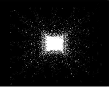
Refer to caption
Refer to caption

(a)(b)

Figure 2. Subsampling maps for Fourier measurements with 5% subsampling with sampling set ΔJsubscriptΔ𝐽\Delta_{J}: (a) Subsampling map for our directional sampling scheme – for this, we take a union of all directional subsampling maps ΔJ,ssubscriptΔ𝐽𝑠\Delta_{J,s}. (b) Subsampling map obtained with variable density sampling for wavelets – see [23] and [15].

5.1.3. Discretization of the Reconstruction Scheme (f,ΔJ)𝑓subscriptΔ𝐽\mathcal{R}(f,\Delta_{J})

Having defined the directional filters Gsdsubscriptsuperscript𝐺𝑑𝑠G^{d}_{s}, we now turn to derive a discretization for implementing our reconstruction scheme (16) and (17). For this, we first let 𝒲Jsubscript𝒲𝐽\mathcal{W}_{J} be the discrete wavelet transform associated with the anisotropic scale matrix Ajsubscript𝐴𝑗A_{j} up to the finest scale j=J𝑗𝐽j=J. For more details on 𝒲Jsubscript𝒲𝐽\mathcal{W}_{J}, we refer to [21].

Next, note that PΨJ,ssubscript𝑃subscriptΨ𝐽𝑠P_{\Psi_{J,s}} in (17) is given as (12), where the basis elements σλsubscript𝜎𝜆\sigma_{\lambda} are obtained by applying the shear operator Sssubscript𝑆𝑠S_{s} for anisotropic wavelets associated with Ajsubscript𝐴𝑗A_{j} for each s𝕊𝑠𝕊s\in\mathbb{S}. Therefore, for a given finite sequence of coefficients c=(cλ)λΛ~J,s𝑐subscriptsubscript𝑐𝜆𝜆subscript~Λ𝐽𝑠c=(c_{\lambda})_{\lambda\in\tilde{\Lambda}_{J,s}}, the wavelet expansion λΛ~J,scλσλsubscript𝜆subscript~Λ𝐽𝑠subscript𝑐𝜆subscript𝜎𝜆\sum_{\lambda\in\tilde{\Lambda}_{J,s}}c_{\lambda}\sigma_{\lambda} can be discretized by Ssd(𝒲J(c))subscriptsuperscript𝑆𝑑𝑠subscriptsuperscript𝒲𝐽𝑐S^{d}_{s}(\mathcal{W}^{*}_{J}(c)), where 𝒲Jsubscriptsuperscript𝒲𝐽\mathcal{W}^{*}_{J} is the conjugate transpose of 𝒲Jsubscript𝒲𝐽\mathcal{W}_{J} and 𝒲J𝒲J=𝒲J𝒲J=Isubscript𝒲𝐽subscriptsuperscript𝒲𝐽subscriptsuperscript𝒲𝐽subscript𝒲𝐽𝐼\mathcal{W}_{J}\mathcal{W}^{*}_{J}=\mathcal{W}^{*}_{J}\mathcal{W}_{J}=I.

We are now ready to derive our discrete implementation for (17) as follows. For this, we let u𝑢u be a target image we want to recover from Fourier samples given by y=PΔJ(u)𝑦subscript𝑃subscriptΔ𝐽𝑢y=P_{\Delta_{J}}\mathcal{F}(u). This is then achieved by first applying the discretization of (17) given by

c^s=argmincs1subject to(Gsd)y=PΔJ(Ssd(𝒲J(cs)))formulae-sequencesubscript^𝑐𝑠argminsubscriptnormsubscript𝑐𝑠1subject todirect-productsubscriptsuperscript𝐺𝑑𝑠𝑦subscript𝑃subscriptΔ𝐽subscriptsuperscript𝑆𝑑𝑠subscriptsuperscript𝒲𝐽subscript𝑐𝑠\hat{c}_{s}=\operatorname*{arg\,min}\|c_{s}\|_{1}{\color[rgb]{0,0,0}\quad\text{subject to}\quad}\mathcal{F}(G^{d}_{s})\odot y=P_{\Delta_{J}}\mathcal{F}(S^{d}_{s}(\mathcal{W}^{*}_{J}(c_{s}))) (48)

for each s𝕊J/2𝑠subscript𝕊𝐽2s\in\mathbb{S}_{J/2}, where direct-product\odot is entry-wise multiplication between two vectors. After obtaining coefficient vectors c^ssubscript^𝑐𝑠{\color[rgb]{0,0,0}\hat{c}_{s}} from (48), we then combine those coefficient sequences by the discrete version of (16) given as

u^=s𝕊J/2G~sdSsd(𝒲J(c^s)),^𝑢subscript𝑠subscript𝕊𝐽2subscriptsuperscript~𝐺𝑑𝑠subscriptsuperscript𝑆𝑑𝑠subscriptsuperscript𝒲𝐽subscript^𝑐𝑠\hat{u}=\sum_{s\in\mathbb{S}_{J/2}}\tilde{G}^{d}_{s}\star S^{d}_{s}(\mathcal{W}^{*}_{J}(\hat{c}_{s})),

to obtain the reconstructed image u^^𝑢\hat{u}.

5.2. Comparison with other Schemes

We now compare our directional sampling scheme with the wavelet based sampling scheme in [23] as well as a shearlet based sampling scheme. For the second scheme, we take a standard shearlet system as implemented in ShearLab [20] with the same Fourier measurements we used for our directional sampling scheme, i.e., we solve

mingΨJg1subject toPΔJ((ug))=0,subscript𝑔subscriptnormsubscriptΨ𝐽𝑔1subject tosubscript𝑃subscriptΔ𝐽𝑢𝑔0{\color[rgb]{0,0,0}\min_{g}\|\Psi_{J}g\|_{1}{\color[rgb]{0,0,0}\quad\text{subject to}\quad}P_{\Delta_{J}}(\mathcal{F}(u-g))=0,}

where ΨJsubscriptΨ𝐽\Psi_{J} is the shearlet transform up to scale J𝐽J. To be more precise, we consider the following sampling schemes:

  • shear08: Our directional sampling scheme with 8 directional filters. The redundancy of the associated shearlet system is 8.

  • shear16: Our directional sampling scheme with 16 directional filters. The redundancy of the associated shearlet system is 16.

  • shear: Shearlet based sampling scheme with a usual shearlet system and the same subsamplng map as one used for our directional sampling scheme. For this, we used a shearlet system with 4 4 8 8 directions across scales, which leads to a redundancy of 25.

  • wave01: Wavelet based sampling scheme with a subsampling map obtained by variable density sampling – see [23] and [15].

  • wave02: Wavelet based sampling scheme with the same subsampling map as the one used for our directional sampling scheme.

All schemes are implemented in MATLAB and tested on a CPU 2.7GHz with 4.00GB memory. Figure 2 illustrates each of the subsampling maps for directional sampling and variable density sampling. The directionality becomes very evident in Figure 2(a) as compared to (b).

Figure 3 shows PSNR values and running times for each of the sampling schemes for two test images. It is evident that our directional sampling schemes shear08 and shear16 consistently outperform the wavelet based sampling schemes wave01 and wave02 in terms of PSNR, while the running time of one of our directional sampling schemes, shear08 is comparable with wavelet based sampling schemes. Moreover, with respect to PNSR our new sampling scheme shear16 slightly outperforms the sampling scheme using the standard shearlets shear, but its running time is significantly faster, in fact about 410 times faster depending on sampling rate.
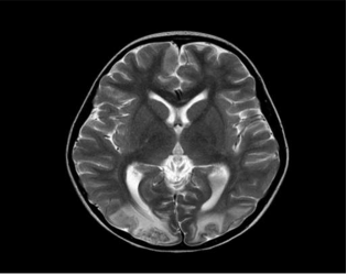
Refer to caption
Refer to caption

(a)(b)
Refer to captionRefer to caption(c)(d)
Refer to captionRefer to caption(e)(f)

Figure 3. (a) 512 ×\times 512 test image A𝐴A. (b) 512 ×\times 512 test image B𝐵B. (c) PSNR values for various sampling schemes for image A𝐴A. (d) PSNR values for various sampling schemes for image B𝐵B. (e) Running time of each of the sampling schemes for image A𝐴A. (f) Running time of each of the sampling schemes for image B𝐵B.

A visual comparison of the reconstruction accuracy is provided in Figure 4. As expected from the previous observations, the shearlet based schemes outperform the wavelet based schemes. In particular, Figure 4 (e)–(f) show that curvilinear edges are much better preserved by using an anisotropic system for reconstruction.
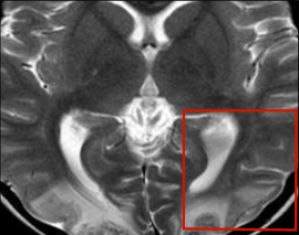
Refer to caption
Refer to caption
Refer to caption

(a)(b)(c)
Refer to captionRefer to captionRefer to caption(d)(e)(f)

Figure 4. Reconstructed images with wavelets and shearlets with our directional sampling using 5% Fourier coefficients for test image A: (a) Original image. (b) wave01: Reconstructed image with wavelets with 27.02dB. (c) shear16: Reconstructed image with our directional sampling scheme with 32.31dB. (d) Original image (Zoom in). (e) wave01: Zoomed image for (b). (f) shear16: Zoomed image for (c).

References

  • [1] B. Adcock, A. C. Hansen, G. Kutyniok, and J. Ma, Linear Stable Sampling Rate: Optimality of 2D Wavelet Reconstructions from Fourier Measurements, SIAM J. Math. Anal. 47 (2015), 1196–1233.
  • [2] B. Adcock, A. C. Hansen, C. Poon, On optimal wavelet reconstructions from Fourier samples: linearity and universality of the stable sampling rate, Appl. Comput. Harmon. Anal. 36 (2013), 387–415.
  • [3] B. Adcock, A. C. Hansen, C. Poon, and B. Roman, Breaking the coherence barrier: A new theory for compressed sensing, preprint.
  • [4] B. Adcock, A. C. Hansen, B. Roman, and G. Teschke, Generalized sampling: stable reconstructions, inverse problems and compressed sensing over the continuum, Adv. in Imag. and Electr. Phys. 182 (2014), 187–279.
  • [5] E. J. Candès and D. L. Donoho, New tight frames of curvelets and optimal representations of objects with piecewise C2superscript𝐶2C^{2} singularities, Comm. Pure Appl. Math. 56 (2004), 216–266.
  • [6] E. J. Candès, J. Romberg and T. Tao, Stable signal recovery from incomplete and inaccurate measurements, Comm. Pure Appl. Math. 59 (2006), 1207–1223.
  • [7] O. Christensen, An Introduction to Frames and Riesz Bases, Birkhäuser, Boston, 2003.
  • [8] I. Daubechies, Ten Lectures on Wavelets, SIAM, Philadelphia, 1992.
  • [9] M. Davenport, M. Duarte, Y. Eldar, and G. Kutyniok, Introduction to Compressed Sensing, in: Compressed Sensing: Theory and Applications, 1–-68, Cambridge University Press, 2012.
  • [10] D. L. Donoho, Sparse components of images and optimal atomic decomposition, Constr. Approx. 17 (2001), 353–382.
  • [11] D. L. Donoho, Compressed sensing, IEEE Trans. Inform. Theory 52 (2006), 1289–1306.
  • [12] D. J. Field, A. Hayes and R. F. Hess, Contour integration by the human visual system: evidence for a local “Association Field”, Vision Res. 33 (1993), 173–193.
  • [13] K. Gröchenig, J. L. Romero, J. Unnikrishnan, and M. Vetterli, On Minimal Trajectories for Mobile Sampling of Bandlimited Fields, Appl. Comp. Harm. Anal., to appear.
  • [14] K. Guo, G. Kutyniok, and D. Labate, Sparse multidimensional representations using anisotropic dilation and shear operators, in: Wavelets and Splines (Athens, GA, 2005), Nashboro Press, Nashville, TN, 2006, 189–201.
  • [15] F. Krahmer and R. Ward, Stable and robust sampling strategies for compressive imaging, IEEE Trans. Image Proc. 23 (2013), 612–622.
  • [16] G. Kutyniok and D. Labate, Introduction to Shearlets, in: Shearlets: Multiscale Analysis for Multivariate Data, 1–38, Birkhäuser Boston, 2012.
  • [17] P. Kittipoom, G. Kutyniok and W.-Q Lim, Construction of compactly supported shearlet frames, Constr. Approx. 35 (2012), 21–72.
  • [18] G. Kutyniok and W.-Q Lim, Compactly supported shearlets are optimally sparse, J. Approx. Theory, 163 (2011), 1564–1589.
  • [19] G. Kutyniok and W.-Q Lim, Dualizable Shearlet Frames and Sparse Approximation, preprint, ArXiv:1411.2303.
  • [20] G. Kutyniok, W.-Q Lim, and R. Reisenhofer, ShearLab 3D: Faithful Digital Shearlet Transforms based on Compactly Supported Shearlets, ACM Trans. Math. Software, to appear.
  • [21] W.-Q Lim, The discrete shearlet transform: A new directional transform and compactly supported shearlet frames, IEEE Trans. Image Proc. 19 (2010), 1166–1180.
  • [22] M. Lustig, D. L. Donoho, and J. M. Pauly, Sparse MRI: The application of compressed sensing for rapid MR imaging, Magn Reson. Med. 58 (2007), 1182–1195.
  • [23] M. Lustig, D. L. Donoho, J. M. Santos, and J. M. Pauly, Compressed Sensing MRI, IEEE Signal Processing Magazine, 25, pp. 72–82, (2008).
  • [24] S. Nam, M. E. Davies, M. Elad, and R. Gribonval, The Cosparse Analysis Model and Algorithms, Appl. Comput. Harmon. Anal. 34 (2013), 30–56.
  • [25] H. Rauhut, Compressive sensing and structured random matrices, in: Theoretical Foundations and Numerical Methods for Sparse Recovery, Radon Series Comp. Appl. Math. 9, 1–92, deGruyter, 2010.
  • [26] J. Shi, W. Yin, A. Sankaranarayanan, and R. Baraniuk, Video Compressive Sensing for Dynamic MRI, preprint.