Neutrino-Driven Convection in Core-Collapse Supernovae: High-Resolution Simulations

Abstract

We present results from high-resolution semi-global simulations of neutrino-driven convection in core-collapse supernovae. We employ an idealized setup with parametrized neutrino heating/cooling and nuclear dissociation at the shock front. We study the internal dynamics of neutrino-driven convection and its role in re-distributing energy and momentum through the gain region. We find that even if buoyant plumes are able to locally transfer heat up to the shock, convection is not able to create a net positive energy flux and overcome the downwards transport of energy from the accretion flow. Turbulent convection does, however, provide a significant effective pressure support to the accretion flow as it favors the accumulation of energy, mass and momentum in the gain region. We derive an approximate equation that is able to explain and predict the shock evolution in terms of integrals of quantities such as the turbulent pressure in the gain region or the effects of non-radial motion of the fluid. We use this relation as a way to quantify the role of turbulence in the dynamics of the accretion shock. Finally, we investigate the effects of grid resolution, which we change by a factor 20 between the lowest and highest resolution. Our results show that the shallow slopes of the turbulent kinetic energy spectra reported in previous studies are a numerical artefact. Kolmogorov scaling is progressively recovered as the resolution is increased.

1. Introduction

The gravitational collapse of the iron core to a proto-neutron star (PNS) marks the last stage of evolution of stars with zero-age main-sequence masses in excess of $\sim 8\ M_{\odot}$. A small ($\sim$ few %) fraction of the enormous amount of gravitational binding energy released in this process ($\sim\textrm{few }\times 10^{53}\,\mathrm{erg}$) is somehow deposited in the outer layers (with mass-coordinate $\gtrsim 1.5\,M_{\odot}$) of the star and powers some of the most energetic explosions in nature, core-collapse supernovae (CCSNe). However, the exact details of the mechanism responsible for re-processing the available energy, which is mostly released as neutrinos streaming out of the PNS, are still uncertain (Janka et al., 2007, 2012; Burrows, 2013; Foglizzo et al., 2015).

In the standard scenario the gravitational collapse of the iron core is halted by the repulsive component of the nuclear force at densities of a few $\times 10^{14}\ \mathrm{g}\,\mathrm{cm}^{-3}$, the inner core bounces back and launches a strong shock wave in the supersonically infalling outer part of the iron core. However, this initial shock wave does not propagate all the way out of the core. Instead, it loses energy due to neutrinos and photo-dissociation of iron-group nuclei and succumbs to the ram pressure of the infalling outer core material within tens of milliseconds. It turns into a stalled accretion shock at a radius of $\sim 100-200\ \mathrm{km}$. To launch an explosion a mechanism must be operating that revives the stalled shock.

The most commonly proposed mechanism to achieve shock revival is the delayed neutrino mechanism (Bethe & Wilson, 1985). In this mechanism, neutrinos are absorbed in the “gain” layer behind the shock. This is thought to provide the necessary energy to revive and accelerate the shock in a run-away process (Bethe, 1990; Burrows & Goshy, 1993; Pejcha & Thompson, 2012). Whether this mechanism is the one powering core-collapse supernovae (CCSN)e is still uncertain. It is now well established that for most progenitors the mechanism does not work in spherical symmetry (Rampp & Janka, 2000; Liebendörfer et al., 2001; Thompson et al., 2003; Liebendörfer et al., 2005; Sumiyoshi et al., 2005). However, successful explosions have been obtained in multiple dimensions thanks to the development of non-spherical fluid instabilities such as the standing accretion shock instability (SASI) (Blondin et al., 2003; Foglizzo et al., 2007) and neutrino-driven convection (Herant, 1995; Burrows et al., 1995; Janka & Müller, 1996; Foglizzo et al., 2006). These instabilities reduce the critical neutrino luminosity needed for explosion in various ways (more on this below). Neutrino-driven convection, in particular, seems to be the instability most commonly found for exploding or close-to-exploding models in 3D (Dolence et al., 2013; Murphy et al., 2013; Ott et al., 2013; Couch, 2013; Couch & O’Connor, 2014; Takiwaki et al., 2014; Abdikamalov et al., 2015; Melson et al., 2015b; Lentz et al., 2015; Melson et al., 2015a), however 3D SASI-dominated explosions have also been reported at least in simulations employing simplified physics (Hanke et al., 2013; Fernández, 2015; Cardall & Budiardja, 2015).

In this context, turbulence generated by buoyancy, SASI (Blondin & Mezzacappa, 2007; Endeve et al., 2012) and/or perturbations in the accretion flow (Couch & Ott, 2013; Müller & Janka, 2015; Couch et al., 2015), is expected to have an important role by providing additional effective pressure support behind the shock (Burrows et al., 1995; Murphy et al., 2013; Couch & Ott, 2015; Radice et al., 2015). At the same time, a full understanding of neutrino-driven convection is still missing. Previous studies were limited either because they were in 2D, (e.g., Murphy & Meakin 2011; Fernández et al. 2014), or because they did not have a sufficient resolution to fully resolve the turbulent dynamics (e.g., Hanke et al. 2012; Takiwaki et al. 2012; Dolence et al. 2013; Couch & O’Connor 2014; Handy et al. 2014; Couch & Ott 2015; Abdikamalov et al. 2015; Melson et al. 2015b; Cardall & Budiardja 2015). The former are probably affected by artefacts related to the symmetry assumptions due to the unphysical inverse cascade in 2D turbulence. The latter might instead be affected by systematic errors that are difficult to quantify without a resolution study spanning a large range of resolutions. The studies of Abdikamalov et al. (2015) and Radice et al. (2015) suggest that convection in current CCSN simulations is under-resolved and dominated by the so-called bottleneck effect, a phenomenon that arises when numerical viscosity suppresses some of the non-linear interactions of the energy cascade and results in the accumulation of kinetic energy at large scale (Yakhot & Zakharov, 1993; She & Jackson, 1993; Falkovich, 1994; Verma & Donzis, 2007; Frisch et al., 2008). This could result in low-resolution simulations being artificially more prone to explosion, as also observed in previous studies (Hanke et al., 2012).

In this study, we aim at increasing the understanding of the role of turbulent neutrino-driven convection in CCSNe and at identifying the key effects responsible for the global dynamics of the accretion flow in a controlled environment and with well resolved simulations. We develop a neutrino driven convection model that is simple enough to allow us to perform 3D simulations at unprecedented resolution, while including all of the basic physics ingredients of a realistic CCSN model: an accretion shock, the converging radial geometry, gravity, neutrino cooling, and neutrino heating.

The rest of the paper is organized as follows. First, in Section 2, we present the details of our neutrino-driven convection model and a description of the numerical methods we employ for our numerical investigation. The general evolution and features of our runs are discussed in Section 3. There, we focus on the dynamics of large scale quantities, such as the average shock radius and entropy profiles. In Section 4, we study the dynamics of convection. In particular, we focus on the role of convection in transporting energy and momentum through the gain region. Section 5 is dedicated to the turbulent energy cascade and to the role of turbulence in providing an effective additional pressure support in the postshock region. We discuss the turbulent cascade and the kinetic energy spectrum of neutrino-driven turbulent convection in Section 6. Finally, we summarize and conclude in Section 7. The appendices contain additional technical details of our model. Appendix A describes our treatment of nuclear dissociation at the shock and Appendix B contains the details of the construction of our initial conditions.

Throughout this paper we use a system of units such that $G=c=M_{\mathrm{PNS}}=1$, $M_{\mathrm{PNS}}$ being the PNS gravitational mass. Where CGS values are quoted, it is to be intended that they correspond to the fiducial case with $M_{\mathrm{PNS}}=1.3\ M_{\odot}$.

2. Methods

In the following, we present the details of our approach and of the employed numerical methods. We note that the aim of our work is not to develop a realistic explosion model. Rather we want to construct a controlled setup containing all of the most important ingredients present in nature and in state-of-the-art global simulations.

2.1. Neutrino-Driven Convection Model

Our initial conditions describe a stalled shock in the core of a massive star at a given radius $r_{s}$. We study the accretion flow in a 3D spherical wedge domain with a $90^{\circ}$ opening angle. The PNS is excised and replaced by an inner boundary condition at a fixed radius, $r_{\mathrm{PNS}}$.

The accretion flow is described by the equations of general relativistic hydrodynamics,

$$\nabla_{\mu}J^{\mu}=0\,, \nabla_{\nu}T^{\mu\nu}=L^{\mu}\,,$$ (1)

where

$$J^{\mu}=\rho u^{\mu}\,, T^{\mu\nu}=[\rho(1+\epsilon)+p]u^{\mu}u^{\nu}+pg^{\mu\nu}\,,$$ (2)

and $L^{\mu}$ is a term that we include to model neutrino heating and cooling (see below). $\rho$, $u^{\mu}$, $p$, $\epsilon$ and $g^{\mu\nu}$ denote the fluid rest-mass density, four-velocity, pressure, specific internal energy and the spacetime metric.

The equation of state (EOS) that we employ is a modified gamma-law EOS

$$p=(\gamma-1)\rho\tilde{\epsilon}\,,$$ (3)

where $\gamma=4/3$ is appropriate for a radiation-pressure dominated gas and $\tilde{\epsilon}$ represents the amount of specific “thermal energy” available after nuclear binding energy has been removed from $\epsilon$ for dissociated nuclei. We account for nuclear dissociation energy in a parametrized way similar to Fernández & Thompson (2009b, a). See Appendix A for the details of our implementation.

The specific entropy for our equation of state is defined up to a constant, so we exploit this to choose the zero of entropy following Foglizzo et al. (2006)

$$s=\frac{1}{\gamma-1}\log\bigg{[}\frac{p}{p_{1}}\Big{(}\frac{\rho_{1}}{\rho}\Big{)}^{\gamma}\bigg{]},$$ (4)

where $\rho_{1}$ and $p_{1}$ are, respectively, the initial postshock density and pressure (see Appendix B). In this way, $s$ is exactly zero at the location of the shock in the initial data.

The gravity of the PNS is included, while self-gravity of the accretion flow is neglected, i.e. we use the Cowling approximation, so that the spacetime metric is constant in time and given by

$$\mathrm{d}\,s^{2}=-\alpha^{2}(r)\,\mathrm{d}t^{2}+A^{2}(r)\,\mathrm{d}r^{2}+r^{2}\mathrm{d}\Omega^{2},$$ (5)

where $\mathrm{d}\,s^{2}$, not to be confused with the entropy, denotes the spacetime line element, $\mathrm{d}\Omega^{2}$ is the line element of the two-sphere and

$$\alpha^{2}=A^{-2}=1-\frac{2M_{\mathrm{PNS}}}{r}.$$ (6)

Neutrino heating and cooling is modeled using the light-bulb scheme introduced by Houck & Chevalier (1992); Janka (2001) and later used in many studies of CCSNe, the most recent being Cardall & Budiardja (2015). The functional form of $L^{\mu}$ that we use is similar to that of Fernández & Thompson (2009a), with the appropriate general-relativistic corrections:

$$L^{\mu}=u^{\mu}\mathcal{L}=u^{\mu}C\rho\bigg{[}f_{\mathrm{heat}}\big{(}Kp_{1}\big{)}^{3/2}\Big{(}\frac{r_{s}}{r}\Big{)}^{2}-p^{3/2}\bigg{]}e^{-\big{(}[s+s_{\mathrm{ref}}]_{-}\big{)}^{2}}\,,$$ (7)

where $C$ is an overall normalization constant, $p_{1}$ is the post-shock pressure, $K$ measures the strength of the heating, $r_{s}$ is the shock radius and we use the notation

$$[X]_{-}=\begin{cases}|X|,&\textrm{if }X<0,\\ 0,&\textrm{otherwise.}\end{cases}$$ (8)

$f_{\mathrm{heat}}$ is set to one for most simulations and when computing the initial conditions. We run some additional models with $f_{\mathrm{heat}}=0.9,0.95,1.05$, and $1.1$ (see Table 1 for more details). In Equation (7) we use a Gaussian cutoff of the heating/cooling term to avoid catastrophic cooling on the surface of the PNS and to suppress heating ahead of the shock. The reference entropy $s_{\mathrm{ref}}$ is chosen to ensure that heating is not switched off when the shock expands and $s$ becomes slightly negative. In our simulations we find (empirically)

$$s_{\mathrm{ref}}=\frac{1}{\gamma-1}\ln 2$$ (9)

to perform well and avoid any artificial suppression of the heating in the gain region. Note that our heating prescription neglects the non-linear feedback between accretion and neutrino luminosity. As such, our scheme might not be appropriate in regimes where the accretion rate at the base of the flow shows significant variations. However, it should be reasonably adequate for the study of nearly steady-state neutrino-driven convection we perform here.

Table 1Key Simulation Parameters.

Run	$f_{\mathrm{heat}}$	$\Delta r\ [\mathrm{m}]$	$\Delta\theta=\Delta\varphi\ [\mathrm{deg}]$
Ref.	$1.0\phantom{0}$	$3839$	$1.8\phantom{0}$
2x	$1.0\phantom{0}$	$1919$	$0.9\phantom{0}$
4x	$1.0\phantom{0}$	$\phantom{0}960$	$0.45$
6x	$1.0\phantom{0}$	$\phantom{0}640$	$0.3\phantom{0}$
12x	$1.0\phantom{0}$	$\phantom{0}320$	$0.15$
20x	$1.0\phantom{0}$	$\phantom{0}191$	$0.09$
F0.9-Ref.	$0.9\phantom{0}$	$3839$	$1.8\phantom{0}$
F0.95-Ref.	$0.95$	$3839$	$1.8\phantom{0}$
F1.05-Ref.	$1.05$	$3839$	$1.8\phantom{0}$
F1.1-Ref.3	$1.1\phantom{0}$	$3839$	$1.8\phantom{0}$
F1.1-2x3	$1.1\phantom{0}$	$1919$	$0.9\phantom{0}$
F1.1-6x3	$1.1\phantom{0}$	$\phantom{0}640$	$0.3\phantom{0}$
F1.1-12x3	$1.1\phantom{0}$	$\phantom{0}320$	$0.15$
1D	$1.0\phantom{0}$	$\phantom{0}640$	$-$
F1.1-1D	$1.1\phantom{0}$	$\phantom{0}640$	$-$

Neutrino heating and cooling is consistently included in the generation of the initial conditions with $f_{\mathrm{heat}}$ set to one. Our initial model is uniquely identified by the PNS radius $r_{\mathrm{PNS}}$, the initial shock position $r_{s}$, the accretion rate $\dot{M}$ and the heating parameter $K$. $C$ is fixed by the condition $\upsilon^{r}(r_{\mathrm{PNS}})=0$, where $\upsilon^{i}$ is the fluid three-velocity. Note that, since our EOS is scale free, the PNS mass, $M_{\mathrm{PNS}}$, scales out of the problem and our results can be applied to any PNS mass with the proper rescaling. The results that we quote are for the fiducial case $M_{\mathrm{PNS}}=1.3\ M_{\odot}$. In particular, the parameters used in this work are $r_{\mathrm{PNS}}=30$ ($\simeq 57\ \mathrm{km}$), $r_{s}=100$ ($\simeq 191\ \mathrm{km}$) and $\dot{M}=10^{-6}$ ($\simeq 0.2\ M_{\odot}\,\mathrm{s}^{-1}$). $K$ is set to $9$ and, correspondingly the equilibrium $C$ is found to be $C=9\times 10^{9}$, which, for our models, corresponds to a luminosity in both the electron or anti-electron neutrinos of

$$L_{\nu}\simeq 1.22\times 10^{52}\left(\frac{12\ \mathrm{MeV}}{T_{\nu}}\right)^{2}\frac{\mathrm{erg}}{\mathrm{s}}\,,$$ (10)

where $T_{\nu}$ is the temperature at the neutrinosphere in $\mathrm{MeV}$. $T_{\nu}$ needs not to be specified by our heating/cooling prescription, because our heating prescription depends only on the total neutrino luminosity and not separately on the neutrino number fluxes and average energies as would have been the case for a real transport scheme. Finally, a small random perturbation with relative amplitude $10^{-6}$ is added to the density field to break the symmetry. The details of the construction of the initial conditions are given in Appendix B.

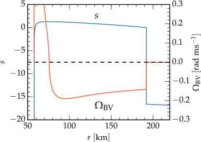
An important parameter for quantifying the convective (in)stability of the initial conditions is the Brunt-Väisäla frequency, $\Omega_{\mathrm{BV}}$, which we write in terms of the quantity (Foglizzo et al., 2006)

$$C_{\mathrm{BV}}=\frac{\gamma-1}{\gamma}g\partial_{r}s\,,$$ (11)

where $g$ is the gravitational acceleration, which we approximate as $M_{\mathrm{PNS}}/r^{2}$. We define

$$\Omega_{\mathrm{BV}}=\sqrt{|C_{\mathrm{BV}}|}\mathrm{sign}(C_{\mathrm{BV}})\,.$$ (12)

With our convention, negative values of $\Omega_{\mathrm{BV}}$ correspond to unstable stratification and $|\Omega_{\mathrm{BV}}|$ gives the growth rate of radial perturbations.

In the case of CCSNe, an additional condition for convective instability is that the growth rate of perturbations should be high enough so that they can reach non-linear amplitudes and become buoyant before being advected out of the gain region by the radial background flow (Foglizzo et al., 2006). This can be quantified by measuring the ratio between the two timescales,

$$\chi=\int\frac{[\Omega_{\mathrm{BV}}]_{-}}{|\upsilon^{r}|}\ \mathrm{d}r\,,$$ (13)

where the integral is extended over the gain region and we have once again used the notation of Equation (8). Foglizzo et al. (2006) showed that if $\chi\gtrsim 3$ perturbations have enough time to develop large-scale convection. Our simulations have an initial value of $\chi=5.33$, so we expect them to develop large-scale convection.

2.2. Simulation Setup

The Equations (1) are solved on a uniform spherical grid in flux-conservative form (Banyuls et al., 1997), using the 5th order MP5 finite difference high-resolution shock-capturing (Suresh & Huynh, 1997) scheme as implemented in the WhiskyTHC code (Radice & Rezzolla, 2012; Radice et al., 2014). WhiskyTHC employs a linearized flux-split method with carbuncle and entropy fix that makes full use of the characteristic structure of the general relativistic hydrodynamics equations with very small numerical dissipation.

Our computational domain covers the region $57\ \mathrm{km}\lesssim r\lesssim 442\ \mathrm{km}$ ($825\ \mathrm{km}$ for models with $f_{\mathrm{heat}}\geq 1.05$), $\pi/4<\theta<3\pi/4$ and $-\pi/4<\varphi<\pi/4$. We use reflecting boundary conditions at the inner boundary, inflow conditions at the outer boundary, and impose periodicity in the angular directions. To ensure a constant accretion rate through the shock, we add artificial dissipation, using a standard 2nd order prescription, close to the outer boundary, always outside of the shock front, to some of the low-resolution runs. Dissipation is found not to be necessary for the 4x, 12x, and 20x runs. In the other simulations, instead, we find dissipation to be necessary to prevent oscillations in the fluid quantities close to the outer boundary that, if not suppressed, can alter the accretion rate by a few percent. The grid spacing for the reference resolution is $\Delta r\simeq 3.8\ \mathrm{km}$, $\Delta\theta=\Delta\varphi=1.8^{\circ}$. The reference resolution is similar to the one employed in recent radiation-hydrodynamics simulations (Melson et al., 2015b; Lentz et al., 2015). For the other resolutions we refined the grid relative to the reference run by factors $2,4,6,12,20$, i.e. up to $\Delta r\simeq 190\ \mathrm{m}$ and $\Delta\theta=\Delta\varphi=0.09^{\circ}$ for the 20x run. All of the simulations are carried out until $\simeq 640\ \mathrm{ms}$, apart from the 20x and the F1.1 runs. We start the 20x at $\simeq 317\ \mathrm{ms}$ from a snapshot of the 12x run and follow it for only $\simeq 60\ \mathrm{ms}$ due to its high computational cost. We stop the F1.1-Ref., F1.1-6x, and F1.1-12x runs at times $t\simeq 384\ \mathrm{ms}$, $t\simeq 560\ \mathrm{ms}$ and $t\simeq 566\ \mathrm{ms}$, when the shock reaches the outer boundary of the computational domain. Finally, we perform two additional runs in spherical symmetry at the same (radial) resolution as the 6x resolution. The main characteristics of our runs are summarized in Table 1.

3. Overall dynamics

3.1. Shock evolution

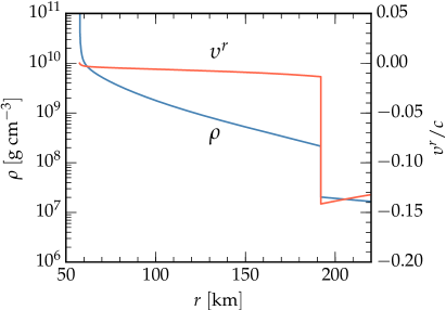
The overall dynamics of our runs is best summarized by the average shock radius evolution, shown in Figures 1 and 2. The dynamics consist in an initial transient lasting $\simeq 25\ \mathrm{ms}$ where the shock radius first expands and then recedes. This transient is triggered by waves reflecting on the surface of the PNS, where the initial conditions are necessarily an approximation to the real steady state solution, which predicts infinite density and zero velocity at the surface of the PNS (this is an artifact arising due to the assumption of stationarity, see Appendix B).

Figure 1.— Average shock radius evolution for all runs with $f_{\mathrm{heat}}=1$. After an initial transient, the shock radius expands as convection develops. For the fiducial model, the growth slows down significantly and quasi-periodic oscillations appear when the convective plumes start to interact non-linearly with the shock front. The black dashed line shows the shock radius for a reference 1D run.

Figure 2.— Average shock radius evolution for runs with enhanced heating. After the initial transient, the shock radius immediately starts to expand. The expansion is not significantly accelerated when the shock reaches large radii (as it would be in a full-physics simulations) partly because of our very simplified treatment of nuclear dissociation, with a constant specific energy loss for each fluid element crossing the shock. In a more realistic simulation, the amount of energy loss drops with radius and this leads to an accelerated expansion. The deviations between the reference resolution and the high resolution simulations are much more pronounced than for the case without enhanced heating (c.f. Figure 1). The black dashed line shows the shock radius for a reference 1D run.

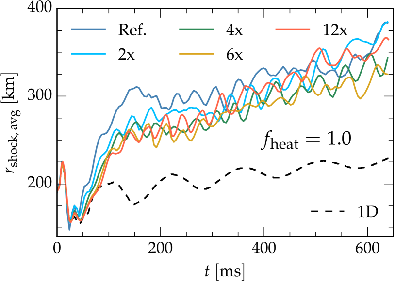
For the fiducial case with $f_{\mathrm{heat}}=1.0$, after the initial transient, turbulence starts to develop: the initial seed perturbations trigger the formation of small buoyant plumes at the base of the gain layer. These plumes grow as they find their way to the shock and convection gains strength. After $t\simeq 150\ \mathrm{ms}$ the entropy perturbations are strong enough to cause large deformations of the shock front.

When the plumes start to interact strongly with the shock at $t\gtrsim 150\ \mathrm{ms}$, the dynamics becomes fully non-linear and characterized by a slow growth of the shock radius and quasi-periodic oscillations with period of the order of the advection timescale (see below). Until this point the different runs appear to be monotonically convergent, with high-resolution simulations having smaller average shock radii. However, as soon as the dynamics becomes fully non-linear their shock radius evolutions lose point-wise convergence, although the evolutionary tracks of all of the runs are broadly consistent with each other.

By comparison, the evolution of our 1D run, also shown in Figure 1, is rather uneventful. The 1D run shows the same initial transient as the 3D data, but afterwards it starts oscillating around its original position and shows only a modest secular growth, which is mainly driven by the accumulation of material in the gain region and continues for the whole duration of the simulation. This shows that the growth of the shock radius after $t\simeq 75\ \mathrm{ms}$ and up to $t\simeq 100\ \mathrm{ms}$ is due to the initial development of convection, which is well captured by our runs.

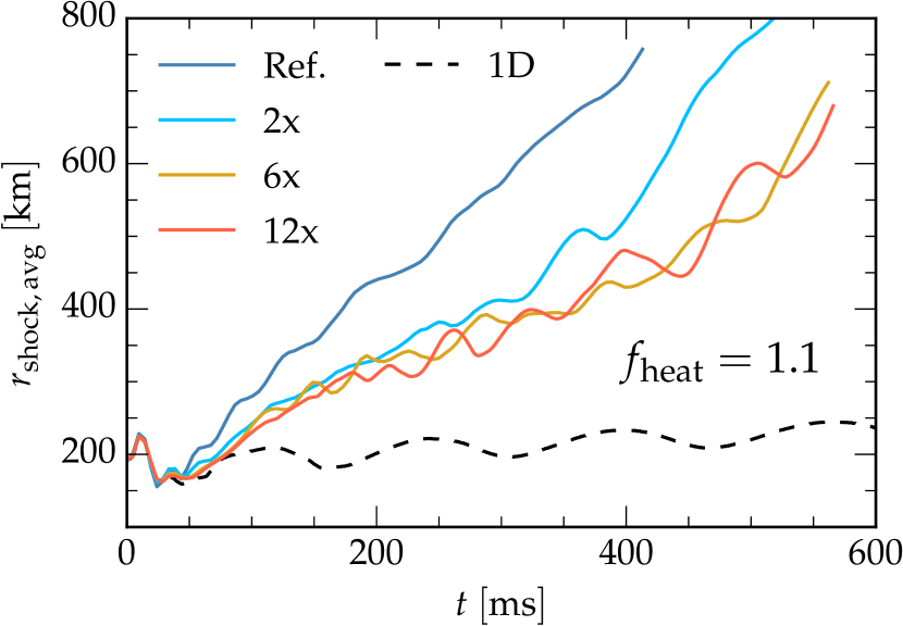
The dynamics of the shock and its behavior with resolution change rather drastically for models with enhanced heating. This can be seen in Figure 2, where we show the average shock radius for the simulations with $f_{\mathrm{heat}}=1.1$. The reference resolution simulation starts to diverge from the 6x and 12x resolutions as soon as the initial transient is over. The 2x resolution seems to be closer to the higher resolution runs, which appear to be converged, but eventually also diverges away after $t\simeq 300\ \mathrm{ms}$. Finally, the 6x and 12x resolutions appear to be consistent with each other for the entire simulated time.

Figure 3.— Entropy, normalized as in Equation (4), in the $xz-$plane at the common time $t\simeq 365\mathrm{ms}$ for the simulations with $f_{\mathrm{heat}}=1.0$. Clockwise from the top left: reference resolution, $2x$, $4x$, $6x$, $12x$ and $20x$ resolutions. The reference resolution is characterized by the presence of a few very large high-entropy plumes. As the resolution increases the topology of the flow becomes more complex and dominated by smaller scale features. At very high-resolutions plumes tend to lose coherency as small-scale turbulent mixing becomes effective at removing sharp features in the entropy.

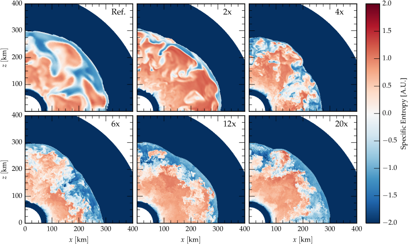
Going back to the fiducial case without enhanced heating, the qualitative differences between resolutions are particularly evident in the visualizations of the fluid entropy. This is shown in Figure 3, where we display the color coded entropy in the $xz-$plane at a representative time ($t\simeq 365\ \mathrm{ms}$). Compared with the other resolutions, the reference resolution shows larger plumes and higher entropies. At this resolution, the dynamics is characterized by the motion of few large structures, while, at higher resolutions, the dynamics appears to be characterized by smaller structures evolving on shorter timescales. Note that the appearance of large scale coherent plumes is typically observed at the onset of explosion (Dolence et al., 2013; Fernández et al., 2014; Müller & Janka, 2015; Lentz et al., 2015). This suggests that, as has been also observed by Hanke et al. (2012); Abdikamalov et al. (2015) and consistently with what we find for the simulations with enhanced heating, low resolution could artificially ease the explosion (see also Couch 2013). On the other hand, note that the 12x resolution, which is the highest for which we carry out a long term evolution, is also the one showing the highest average shock radius growth rate (Figure 1), suggesting that turbulence has a more complex role than simply destroying large-scale plumes.

As the resolution increases, first, secondary instabilities in the flow drive down the size of the typical plumes and create more complex flow structures. Second, at the highest resolutions (12x and 20x), plumes start to lose their coherence due to the presence of small-scale turbulent mixing. Instead of being characterized by entropy “bubbles” with sharp entropy gradients, as in the reference resolution, the flow in high resolution simulations appears to be dominated by the appearance and disappearance of large hot “clouds”, i.e. entropy structures with a complex topology. An animation of the entropy on the equatorial plane for the Ref., 2x, 4x, and 12x resolutions is included in the online supplemental materials.

Figure 4.— Top panel: ratio of the advection timescale (Equation 14) to heating timescale (Equation 16). Middle panel: heating timescale. Bottom panel: advection timescale. $f_{\mathrm{heat}}=1.0$ for all of the runs shown in this figure. As it is the case for the shock radius evolution, also in the heating efficiency our simulations appear to be closely convergent until $t\simeq 100\ \mathrm{ms}$. Afterwards convergence is not monotonic, but all the runs are still in good agreement with each other, especially for $\tau_{\mathrm{adv}}$. The heating timescale shows a somewhat larger spread.

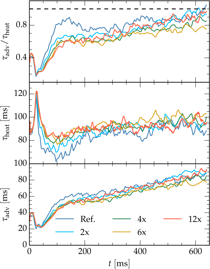
Another commonly employed diagnostic in CCSN simulations is the ratio between the timescale for the advection of a fluid element through the gain layer and the time necessary for it to absorb enough energy from neutrinos to become unbound.

Specifically, the advection timescale is typically defined as (Fernández, 2012; Müller et al., 2012)

$$\tau_{\mathrm{adv}}=\frac{M_{\mathrm{gain}}}{\dot{M}}\,,$$ (14)

where $\dot{M}$ is the accretion rate, $M_{\mathrm{gain}}$ is the total mass in the gain region

$$M_{\mathrm{gain}}=\int\rho W\sqrt{\gamma}\mathrm{d}V\,,$$ (15)

where $W$ is the Lorentz factor, $\sqrt{\gamma}$ is the spatial volume form and the integral is extended over the gain region.

The heating timescale is defined as (e.g., Fernández 2012)

$$\tau_{\mathrm{heat}}=\frac{|E_{\mathrm{bind}}|}{\dot{Q}_{\mathrm{net}}}\,,$$ (16)

where $E_{\mathrm{bind}}$ is the binding energy of the gain region, which we compute as in (Müller et al., 2012):

$$E_{\mathrm{bind}}=\int\big{\{}\alpha[\rho(1+\tilde{\epsilon}+p/\rho)W^{2}-p]-\rho W^{2}\big{\}}\sqrt{\gamma}\mathrm{d}V\,.$$ (17)

$\dot{Q}_{\mathrm{net}}$ is the net heating/cooling rate

$$\dot{Q}_{\mathrm{net}}=\int W\mathcal{L}\sqrt{\gamma}\,\mathrm{d}V\,,$$ (18)

where $\sqrt{\gamma}$ is the determinant of the spatial metric and the integrals in the previous equations are extended over the gain region.

The advection and heating timescales as well as their ratio for the fiducial model ($f_{\mathrm{heat}}=1.0$) are shown in Figure 4. In a similar way to what we see for the average shock radius, we find that the different runs are monotonically convergent during the first $\sim 100\ \mathrm{ms}$. Afterwards, the various simulations have consistent trends, but there is no point-wise convergence. After the initial transient, starting from $t\simeq 50\ \mathrm{ms}$, the advection timescale grows by roughly a factor $2$ as convection develops. Then, starting from $t\simeq 100\ \mathrm{ms}$ the advection timescale shows a secular growth, due to the increase of the mass in the gain region and it reaches $\sim 80\ \mathrm{ms}$ toward the end of the simulations. At the same time, the heating timescale remains roughly constant, especially at high resolution, and the runs slowly approach the approximate condition for explosion, $\tau_{\mathrm{adv}}\lesssim\tau_{\mathrm{heat}}$ (Murphy & Burrows, 2008; Marek & Janka, 2009; Fernández, 2012; Müller et al., 2012).

If we consider the ratio $\tau_{\mathrm{adv}}/\tau_{\mathrm{heat}}$ as a way to measure the proximity of the simulations to explosion, we can see from Figure 4 that, for the first $\sim 300\ \mathrm{ms}$, high resolution simulations are indeed further away from explosion than low resolution simulations as observed by Hanke et al. (2012) and Abdikamalov et al. (2015) (although this trend seems to be reversed at very high resolutions). Whether this results in explosions being triggered artificially or not at low resolution will likely depend on how close the models are to explosion. For instance, Abdikamalov et al. (2015) found finite-resolution effects to be small for non-exploding models and comparatively large for exploding models. Similarly, in our simplified setup we also find the evolution of models with enhanced heating to be more sensitive to resolution (compare Figures 1 and 2). The recent results by Melson et al. (2015a) suggest that full-physics CCSN simulations are close to the critical threshold for explosion. One might speculate that, near criticality, relatively small differences as those documented in Figure 4 could lead to dramatic consequences for some progenitors.

4. Dynamics of Convection

4.1. Convective Energy Transport

One of the characteristics of convection is that it provides a way to transport energy. In the context of neutrino-driven convection in CCSNe it is interesting to consider the role of convection in transporting energy from the bottom of the gain layer, where neutrino deposition is the strongest, outwards, toward the shock and, if an explosion is ultimately launched, by means of the latter, toward the envelope of the star.

Figure 5.— Thermal and kinetic energy transport by the flow for the $f_{\mathrm{heat}}=1.0$ simulations. Left panels: time- and angle-averages of the kinetic and thermal energy radial energy fluxes. Right panels: time- and angle-averages of the turbulent component of the kinetic and thermal radial energy fluxes. $r_{g}$ and $r_{s}$ are the gain and shock radius respectively. The time average excludes the first $t\simeq 192\ \mathrm{ms}$ and it is carried out until the end of the simulation. The gray shaded region shows the standard deviation of the 12x run. Turbulence operates by transporting thermal energy toward larger radii and kinetic energy toward smaller radii.

To analyze the efficiency of neutrino-driven convection for energy transport, we consider the angular-integrated energy equation. Our analysis can be considered as the general-relativistic analog of that of Meakin & Arnett (2007); Murphy & Meakin (2011), with some minor differences. Our starting point is the angle-averaged energy equation on the Schwarzschild background metric, Equation (5)

$$\partial_{t}\langle A\,r^{2}E\rangle+\partial_{r}\langle r^{2}[E+p]\upsilon^{r}\rangle=\mathcal{G}_{E}\,,$$ (19)

where $\mathcal{G}_{E}$ describes heating/cooling by neutrinos and gravity

$$\mathcal{G}_{E}=r^{2}\rho W\mathcal{L}-\big{[}r^{2}(E+p)\upsilon^{r}\big{]}\partial_{r}\log\alpha\,.$$ (20)

The energy density is

$$E=\rho hW^{2}-p\,.$$ (21)

The total energy density can be decomposed as

$$E=\rho hW(W-1)+(\rho\epsilon+p)W+\rho W-p\,,$$ (22)

where we can distinguish the relativistic kinetic energy density

$$K=\rho hW(W-1)\,,$$ (23)

the “Newtonian” enthalpy density

$$H=(\rho\epsilon+p)W\,,$$ (24)

and the rest-mass energy density

$$D=\rho W\,.$$ (25)

The associated radial fluxes are $F_{K}=r^{2}K\,\upsilon^{r}$, $F_{H}=r^{2}H\,\upsilon^{r}$ and $F_{D}=r^{2}D\,\upsilon^{r}$. We can rewrite Equation (19) as

$$\partial_{t}\langle Ar^{2}E\rangle+\partial_{r}\langle F_{K}+F_{H}+F_{D}\rangle=\mathcal{G}_{E}\,.$$ (26)

Furthermore, we decompose the radial velocity into a mean part and a “turbulent” part as

$$\upsilon^{r}=\langle\upsilon^{r}\rangle+\delta\upsilon^{r}\,.$$ (27)

More in general we define the turbulent velocity to be

$$\delta\upsilon^{i}=\upsilon^{i}-\langle\upsilon^{r}\rangle\delta_{r}^{\phantom{r}{i}}\,.$$ (28)

Note that our definition of turbulent velocity is not the standard definition in the turbulence literature, since $\langle\delta\upsilon^{\theta}\rangle$ and $\langle\delta\upsilon^{\phi}\rangle$ are not necessarily exactly zero. On the other hand, since we consider only non-rotating models, it is natural to consider any non-radial fluid motion to be related to turbulence. Moreover, since our background model is spherically symmetric, we expect the ensemble averages of $\delta\upsilon^{\phi}$ and $\delta\upsilon^{\theta}$ to vanish.

In the same way, we can split the fluxes into a mean and turbulent component as

$$F_{u}=\bar{F}_{u}+F_{u}^{\prime}\,,$$ (29)

where $u=K,H$ or $D$, and

$$\bar{F}_{u}=\langle r^{2}u\rangle\langle\upsilon^{r}\rangle\,, F_{u}^{\prime}=\langle r^{2}u\delta\upsilon^{r}\rangle\,.$$ (30)

Finally, the equation for the energy transported by convection can be written as

$$\partial_{t}\langle Ar^{2}E\rangle+\partial_{r}[\bar{F}_{K}+\bar{F}_{H}+\bar{F}_{D}]+\partial_{r}[F_{K}^{\prime}+F_{H}^{\prime}+F_{D}^{\prime}]=\mathcal{G}_{E}\,.$$ (31)

Note that $F_{D}$ is also the flux of the angle-averaged continuity equation

$$\partial_{t}\langle Ar^{2}D\rangle+\partial_{r}\langle F_{D}\rangle=0\,,$$ (32)

so that $\bar{F}_{D}$ and $F_{D}^{\prime}$ can also be interpreted as mean and turbulent contributions to the mass transport:

$$\partial_{t}\langle Ar^{2}D\rangle+\partial_{r}\bar{F}_{D}+\partial_{r}F_{D}^{\prime}=0\,.$$ (33)

Combining Equation (32) with Equation (26), we obtain an equation for the energy density minus the rest-mass energy density,

$$\partial_{t}\langle Ar^{2}[E-D]\rangle+\partial_{r}\langle F_{K}+F_{H}\rangle=\mathcal{G}_{E}\,.$$ (34)

The quantity $E-D$ can be considered as the generalization of the sum of the Newtonian internal and kinetic energy densities of the fluid.

To identify the important terms in the energy equation, we study the radial profiles of the angle-averaged mean and turbulent fluxes of Equation (34). To this end, we re-map the fluxes to be a function of the normalized radius

$$r_{\star}=\frac{r-r_{g}}{r_{s}-r_{g}}\,,$$ (35)

where $r_{g}$ and $r_{s}$ are the average gain and shock radius respectively and we defined the average gain radius, $r_{g}$, to be the radius at which neutrino heating becomes larger than neutrino cooling in an angle-averaged sense. This way the extent of the gain region in terms of the re-scaled radius is $0\leq r_{\star}\leq 1$ and we do not have to worry about secular changes in the shock radius when averaging in time. Next, we average the re-mapped fluxes using data starting at $t=30\,000\ M_{\mathrm{PNS}}\simeq 192\ \mathrm{ms}$ to exclude the initial transient and the development phase of convection and include only the later quasi-steady phase.

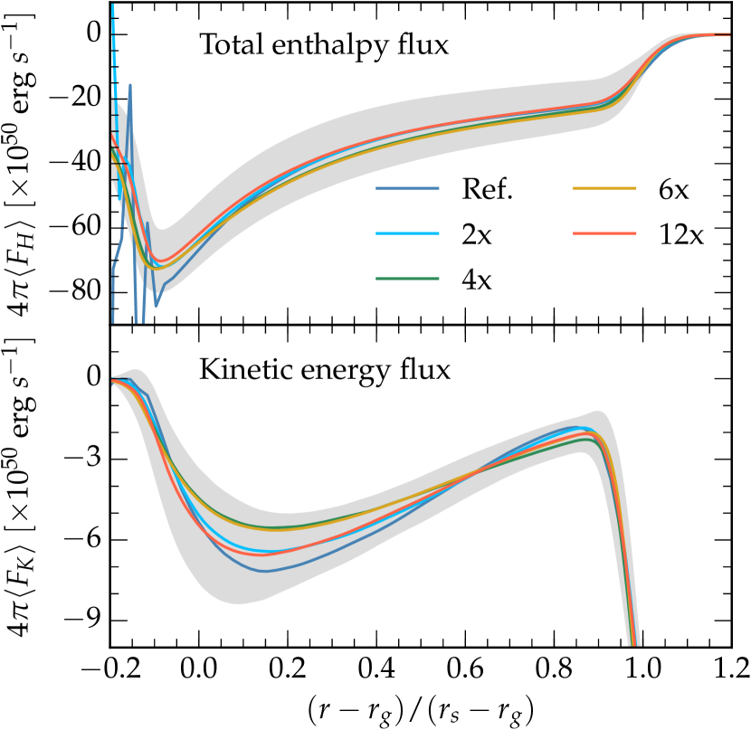
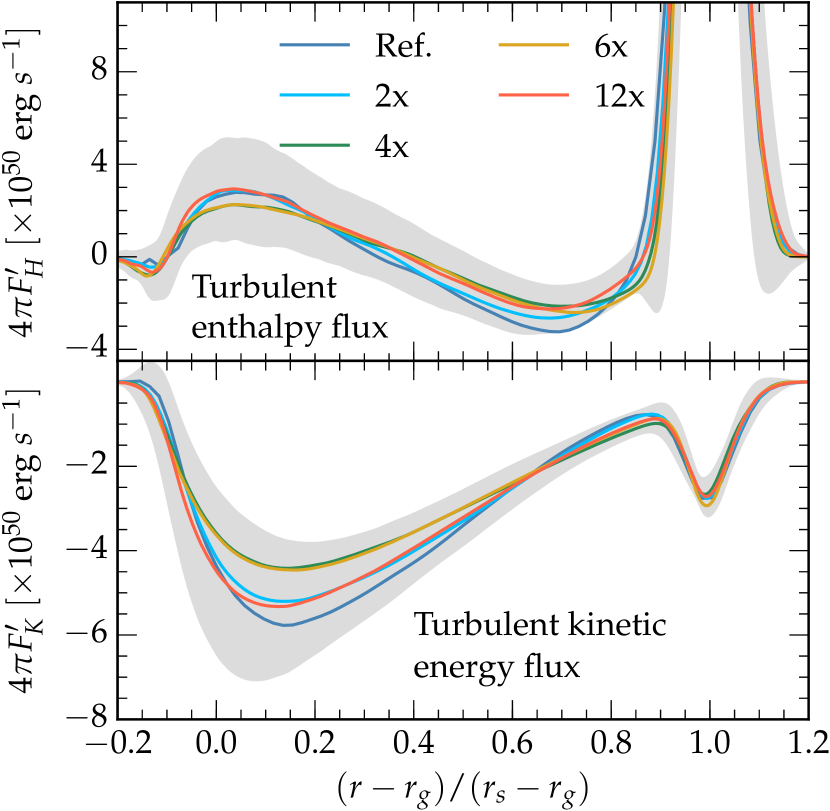
The result of this analysis is portrayed by Figure 5, where we show the angle-averaged total (mean + turbulent) and turbulent kinetic and enthalpy fluxes. In each panel, the gray shaded area shows the standard deviation of the 12x resolution. The other runs show variations of very similar magnitude and we do not show their standard deviations to avoid overcrowding the figure.

The large extent of the gray region in the plots is indicative of the fact that the angle-averaged fluxes, total and turbulent for both kinetic energy and enthalpy, show large variations in time. These are large-scale oscillations that correlate with the quasi-periodic oscillations we see in the shock radius (Figure 1).

The reference resolution also shows large spatial oscillations in the cooling layer where density and pressure have a steep gradient which is not sufficiently resolved at low resolution. These oscillations are present also for the 2x resolution, but are confined to a much deeper layer close to the PNS and disappear at higher resolution.

The angle-averaged fluxes are shown in the left panels of Figure 5. Both the enthalpy (top) and the kinetic (bottom) energy fluxes are negative. This means that, despite the presence of convection, the energetics of the flow are dominated by advection and there is no net transfer of energy upwards from the gain region to the shock. Note that this might change if the flow transitions to an explosion, see, e.g., (Abdikamalov et al., 2015). In the stalled shock phase, however, turbulence can only act in such a way as to decrease (in absolute value) the mean fluxes and favor the accumulation of mass and energy in the gain region, which is a necessary condition for shock expansion (Janka, 2001). Finally, from the amplitude of the fluxes upstream of the shock, we can also see that, as expected, kinetic energy is the main form with which energy is accreted through the shock, but most of it is converted into thermal energy by the shock.

The turbulent fluxes are shown in the right panels of Figure 5. The angle-averaged turbulent enthalpy flux is positive at the base of the gain region, while the angle-averaged turbulent kinetic energy flux is negative everywhere. This is the result of buoyant plumes driving thermal energy upwards and displacing lower entropy gas which is pushed downwards in a process that converts thermal energy back into kinetic energy.

An important point that we can deduce from Figure 5 is that the total amount of energy transported by turbulence is not particularly large compared to that of the background flow. Even at the base of the gain region, where heating is stronger and the convective enthalpy fluxes are more intense, the turbulent angle-average enthalpy flux is at most a few $\times 10^{50}\ \mathrm{erg}\ \mathrm{s}^{-1}$, which is only of order $10\%$ of the total enthalpy flux. Turbulence does contribute significantly to the total kinetic energy flux, with the turbulent angle-averaged fluxes being $\sim 80\%$ of the total, but kinetic energy is dwarfed by the thermal energy in the energy budged downstream from the shock. Obviously, these values are specific to our accretion model and, for instance, they change by a few percent as we vary $f_{\mathrm{heat}}$ from $0.9$ to $1.1$. However, we do not expect qualitative differences to appear for other models during the stalled accretion shock phase.

Despite the violence of convection and the fact that buoyant plumes impinge violently onto the shock, the total energy fluxes are still dominated by the radial advection flow. This shows that the larger shock radius in multi-dimensional simulations with respect to one-dimensional simulations is not mainly due to the direct transport of energy by convection, which has a measurable, but small overall impact. Turbulence, instead, acts in a more indirect way by slowing down the drain of energy from the region close to the shock.

This effect is analogous to, but distinct from, another well known consequence of neutrino-driven convection: the enhancement of the absorption efficiency due to the increased dwelling time of fluid elements in the gain region (e.g., Burrows et al. 1995; Murphy & Burrows 2008; Fernández & Thompson 2009a).

We remark that the large oscillations shown in Figure 5 in the angle averaged turbulent fluxes at the location of the shock wave are an artefact of our decomposition arising from the fact that the angle averaged velocity picks up values both upstream and downstream of the shock, so that the turbulent velocity, computed according to Equation (28), is artificially large. Obviously, this is only a limitation of our analysis and nothing “special” happens at the location of the shock. This can be confirmed by looking at the total fluxes in the left panels of Figure 5.

Finally, concerning the behavior with resolution, we see that there is no clear monotonic trend with resolution in the fluxes. The low resolution runs (Ref. and 2x) tend to show more vigorous convection (as measured from the magnitude of the turbulent fluxes) than high resolution runs (4x and 6x). However, at very high resolution (12x) convection becomes again as strong as for the low resolution simulations. This is consistent with the behavior of $\tau_{\mathrm{adv}}/\tau_{\mathrm{heat}}$ shown in Figure 4. Note, however, that, given the large time variations of the fluxes, these differences are not at a sufficient level to draw strong conclusions concerning the behavior with resolution. Also, as for the timescales, the differences in the energy fluxes with resolution might become more pronounced for models that are closer to the explosion threshold.

Figure 6.— Time- and angle-averaged entropy profiles for the $f_{\mathrm{heat}}=1.0$ simulations. $r_{g}$ and $r_{s}$ are the gain and shock radius respectively. The time average excludes the first $t\simeq 192\ \mathrm{ms}$ and it is carried out until the end of the simulation. The zero of the entropy is chosen according to Equation (4). Multi-dimensional convection tends to flatten the average entropy profile, with respect to the initial conditions (c.f. Figure 14) or the 1D spherically symmetric simulation. However, convection is not efficient enough to completely cancel out the entropy gradient.

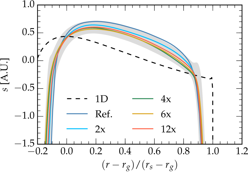
We note that Yamasaki & Yamada (2006) constructed an analytic model to study the effects of convection on the critical luminosity needed for explosion (Burrows & Goshy, 1993) and found, instead, turbulent energy transport due to convection to have a very significant effect. The discrepancy between our results and the model of Yamasaki & Yamada (2006) is due to the fact that in their model Yamasaki & Yamada (2006) estimated the turbulent energy fluxes assuming convection to be efficient enough to cancel the unstable gradient in the angle-averaged radial entropy profile. This is, however, not what it is found in simulations. The time- and angle-averaged entropy profiles from our simulations are shown in Figure 6. As for the fluxes, we remap the data to be a function of $r_{\star}$ and then average in time. We find that multi-dimensional convection is able to stabilize (and actually over-stabilize) the average entropy gradient at the base of the gain region and flatten it over most of the gain layer, as compared to the initial data (c.f. Figure 14), or to the 1D simulation. However, convection is not efficient enough to completely remove the unstable stratification and the average entropy profile still has a negative radial gradient over most of the gain region. Similar entropy profiles have also been reported in other simulations with varying degree of sophistication, (e.g., Murphy & Burrows 2008; Hanke et al. 2012; Dolence et al. 2013; Ott et al. 2013). This means that Yamasaki & Yamada (2006) overestimated the turbulent enthalpy fluxes induced by neutrino-driven convection, which, according to simulations are not as large as to cancel the entropy gradient. As a consequence, the model of Yamasaki & Yamada (2006) overestimates the effects of the turbulent energy transport on the critical luminosity.

4.2. Momentum transport

In the light of our previous discussion, we can conclude that thermal energy transport by turbulence appears to be only a $\sim 10\%$ effect. On the other hand, the fact that turbulence dominates the kinetic energy balance suggests that turbulence, and, in particular, turbulent pressure, might have a more important role in the momentum equation. This is indeed what was already suggested in various other studies (Murphy et al. 2013; Couch & Ott 2015; Radice et al. 2015).

Figure 7.— Time- and angle-averaged ratio between the radial turbulent pressure and the thermal pressure for the $f_{\mathrm{heat}}=1.0$ runs. $r_{g}$ and $r_{s}$ are the gain and shock radius respectively. The time average excludes the first $t\simeq 192\ \mathrm{ms}$ and it is carried out until the end of the simulation. Turbulence provides a significant contribution (of the order of $\simeq 30\%$) to the total pressure over most of the gain region and up to the shock, although $R_{r}^{\phantom{r}r}/\langle r^{2}p\rangle$ shows large variations close to the shock where the standard deviation of the pressure becomes of the order of the pressure due to the pressure jump across the shock.

To analyze this effect in detail, similarly to what we have done for the energy Equation (34), we consider the angle averaged radial momentum equation,

$$\partial_{t}\langle r^{2}AS_{r}\rangle+\partial_{r}\langle r^{2}S_{r}\upsilon^{r}\rangle=-\partial_{r}\langle r^{2}p\rangle+\mathcal{G}_{S}\,,$$ (36)

where the radial momentum is $S_{r}=\rho\,h\,W^{2}\,\upsilon_{r}$ and $\mathcal{G}_{S}$ is the term containing geometric, gravitational, and neutrino source terms in the momentum equation

$$\begin{split}\mathcal{G}_{S}=A^{2}r^{2}W^{2}(\upsilon^{r})^{2}\mathcal{L}-\big{[}E+p+S_{r}\upsilon^{r}\big{]}A^{2}+\frac{R_{\theta}^{\phantom{\theta}\theta}+R_{\phi}^{\phantom{\phi}\phi}}{r}+2pr\,,\end{split}$$ (37)

where $R_{i}^{\phantom{i}j}$ is the Reynolds stress tensor, which we define to be

$$R_{i}^{\phantom{i}j}=\langle r^{2}\rho hW^{2}\upsilon_{i}\,\delta\upsilon^{j}\rangle.$$ (38)

The reason for the $r^{2}$ factor in this definition is that this simplifies the notation when considering spherically averaged equations.

The flux term $F_{S}=\langle r^{2}S_{r}\,\upsilon^{r}\rangle$ in the LHS of (36) can also be decomposed in a mean and a turbulent part $F_{S}=\bar{F}_{S}+F_{S}^{\prime}=\langle r^{2}S_{r}\rangle\langle\upsilon^{r}\rangle+\langle r^{2}S_{r}\,\delta\upsilon^{r}\rangle$. So that the momentum equation can be rewritten as

$$\partial_{t}\langle r^{2}AS_{r}\rangle+\partial_{r}\bar{F}_{S}+\partial_{r}F_{S}^{\prime}=-\partial_{r}r^{2}\langle p\rangle+\mathcal{G}_{S}.$$ (39)

We note that $F_{S}^{\prime}=R_{r}^{\phantom{r}{r}}$ is the radial component of the Reynolds stress tensor.

Beside gravity, the two most important components of equation (39) are the turbulent pressure $R_{r}^{\phantom{r}{r}}$ and the thermal pressure $\partial_{r}\langle r^{2}p\rangle$. We find the mean angle-averaged momentum flux $\bar{F}_{S}$ to be contributing only $\sim 10\%$ of the total momentum flux. The remainder is carried by turbulence $F_{S}^{\prime}=R_{r}^{\phantom{r}{r}}$ over most of the gain region.

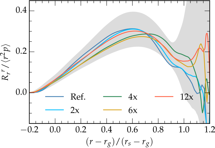
In Figure 7 we show the time- and angle-averaged ratio of the turbulent pressure $R_{r}^{\phantom{r}{r}}$ and the thermal pressure $r^{2}\langle p\rangle$ for our runs. As for the energy fluxes, we time-average the data starting at $t\simeq 192\ \mathrm{ms}$ rescaling them as a function of $r_{\star}$ (Equation 35). The shaded area shows the standard deviation (in time) of the 12x simulation.

We find the turbulent pressure to provide roughly $\sim 30\%$ of the total pressure support over most of the gain region and close to $\sim 20\%$ at the location of the shock in a time-average sense. As highlighted by the shaded region in Figure 7, the ratio of turbulent to thermal pressure does, however, show significant (tens of %) deviations in time. These variations are particularly large close to the shock, because there the pressure has variations of order 1 (given that the pre-shock pressure is negligible). Turbulent pressure support drops near the base of the gain region and in the cooling layer, where turbulence is suppressed by the strong stable stratification near the PNS surface.

Figure 8.— Time- and angle-averaged ratio between the radial turbulent pressure and the thermal pressure as a function of the heating factor $f_{\mathrm{heat}}$ for the reference resolution. $r_{g}$ and $r_{s}$ are the gain and shock radius respectively. The time average excludes the first $t\simeq 192\ \mathrm{ms}$ and it is carried out until the end of the simulation. As the simulations approach the threshold for explosion the turbulent contribution to the total pressure becomes increasingly important.

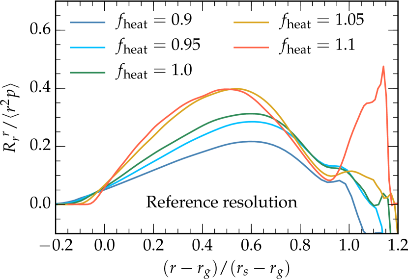
We point out that the ratio of the effective turbulent pressure to the thermal pressure is very sensitive to $f_{\mathrm{heat}}$: as $f_{\mathrm{heat}}$ changes from $0.9$ to $1.1$ at the reference resolution, the maximum of the time-averaged ratio grows from $\sim 20\%$ and saturates at the $\sim 40\%$ level as shown in Figure 8. There we show the time- and angle-averaged ratio of turbulent to thermal pressure for simulations with different heating factors $f_{\mathrm{heat}}$ (see Equation 7) at the reference resolution. The time-average window is the same as for Figure 7. What we find is consistent with what was found by Couch & Ott (2015) who also find the ratio between turbulent pressure and pressure to be significant. In their simulations, at the transition to explosion, the effective pressure support from turbulence exceeds $50\%$ of the thermal pressure.

The behavior with resolution for the ratio between turbulent and thermal pressure is in line with what we find for the energy fluxes or the characteristic timescales. Turbulent support initially appears to decrease with resolution, but rises again at the highest resolution (12x). Obviously, the same caveats discussed in the case of the energy fluxes hold here. The time variations of the ratio between turbulent pressure and pressure, with typical amplitudes of the order of $30\%$, are such that we cannot draw strong conclusions concerning their behavior with resolution based only on the differences we observe. There is, however, a clear correlation between shock radii, enthalpy fluxes and radial Reynolds stresses: large shock radii are found in simulations with high turbulent enthalpy flux and turbulent pressure.

Figure 9.— Time- and angle-averaged radial profiles for radial and tangential Reynolds stresses (Equation 38) for the $f_{\mathrm{heat}}=1.0$ runs. The Reynolds stresses show large time and spatial deviations from their average value. The gray shaded region shows the standard deviation of the 12x run. Turbulence is anisotropic with $R_{r}^{\phantom{r}r}\simeq 2R_{\theta}^{\phantom{\theta}\theta}$ over most of the gain region.

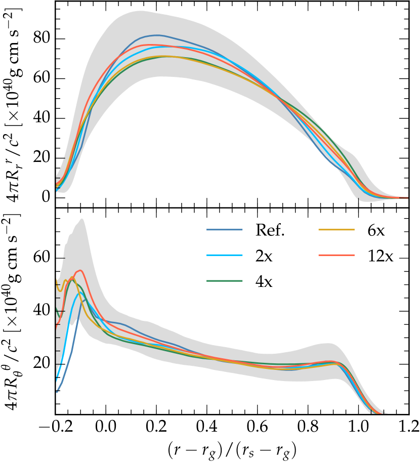
The time- and angle-averaged profiles for the radial and angular components of the Reynolds stresses are shown in Figure 9. We show $R_{r}^{\phantom{r}r}$ and $R_{\theta}^{\phantom{\theta}\theta}$ as a function of the normalized radius $r_{\star}$ (note that since our background model is non-rotating, $R_{\phi}^{\phantom{\phi}\phi}\sim R_{\theta}^{\phantom{\theta}\theta}$). The turbulence is highly anisotropic with $R_{r}^{\phantom{r}r}\sim 2R_{\theta}^{\phantom{\theta}\theta}\sim 2R_{\phi}^{\phantom{\phi}\phi}$ over most of the gain region, with the important exception of the regions close to the shock where there is near equipartition between $R_{r}^{\phantom{r}r}$ and $R_{\theta}^{\phantom{\theta}\theta}$ as also observed in other simulations, see e.g., (Murphy et al., 2013; Couch & Ott, 2015). The angular components of the Reynolds stress also become dominant in the cooling layer, where radial motions are strongly suppressed by the steep stratification.

5. The Effects of Turbulence

We have seen that the effective pressure from turbulence can contribute a significant fraction of the total pressure support in the gain region. However, it is not a-priori clear how to translate this into terms of the global evolution of a CCSN. For example, one may ask the important question of how much the effective pressure from turbulence contributes to the evolution of the shock radius. We address this question in the following by means of a model explaining the shock radius evolution in terms of measurable flow quantities in the gain region.

5.1. Momentum Balance Equation

We are going to derive an equation explaining the influence of turbulence on the shock radius evolution, which will be an extension of the approach introduced by Murphy et al. (2013). They considered the Rankine-Hugoniot conditions for a standing accretion shock in a supernova core. In our notation

$$[F_{S}+r^{2}p]_{d}=[F_{S}+r^{2}p]_{u}\,,$$ (40)

where $u$ and $d$ denote upstream and downstream values, respectively. They showed how these equations could be modified to account for the turbulent pressure. They formally decomposed the momentum flux in a turbulent and average part in Equation (40) to obtain, assuming a purely radial accretion flow upstream from the shock,

$$[\bar{F}_{S}+R_{r}^{\phantom{r}r}+r^{2}p]_{d}=[\bar{F}_{S}+r^{2}p]_{u}\,.$$ (41)

This equation is not entirely rigorous because it uses averaged quantities inside a non-averaged equation, however it has been shown to be well reproduced by the numerical simulations of Murphy et al. (2013) and Couch & Ott (2015). In particular, Couch & Ott (2015) found that the turbulent pressure expressed in this fashion can be up to $50\%$ of the thermal pressure, making a very significant contribution to the momentum balance in Equation (41).

Radice et al. (2015) pointed out that the effective adiabatic index of turbulence, which is related to the efficiency with which turbulent energy density is converted into thermal support, is $\gamma_{\mathrm{turb}}\simeq 2$, which is much larger than the $\gamma=4/3$ of a radiation pressure dominated gas. This makes turbulent energy more “valuable” than thermal energy in the sense that, per unit specific internal energy, turbulent energy contributes a greater effective pressure than thermal energy.

More recently, Murphy & Dolence (2015) extended Equation (40) using the integral form of the momentum and energy equations with the goal of developing a new explosion condition, but they did not include the effects of turbulence in their analysis. See also Gabay et al. (2015) for an alternative approach for the derivation of an explosion condition based on the use of a virial-like relation for the moment of inertia of the accretion layer around the PNS.

Here, we extend the approach of Murphy et al. (2013) in a way similar to Murphy & Dolence (2015), but with the different goal of finding a way to quantify the effects of turbulence on the explosion and not of constructing an explosion diagnostic, which would be inappropriate given the limitations of our model. Similarly to Murphy & Dolence (2015), our starting point is Equation (36). Let us consider two spheres with radius $r_{1}$ and $r_{0}$, with $r_{1}\geq r_{0}$. Then Equation (36) can be integrated between $r_{0}$ and $r_{1}$ to yield

$$\begin{split}\langle F_{S}(r_{1})+r_{1}^{2}p(r_{1})\rangle=\langle&F_{S}(r_{0})+r_{0}^{2}p(r_{0})\rangle+\\ &\int_{r_{0}}^{r_{1}}\langle\mathcal{G}_{S}\rangle\mathrm{d}r-\int_{r_{0}}^{r_{1}}\partial_{t}\langle r^{2}AS_{r}\rangle\mathrm{d}r\,,\end{split}$$ (42)

where $\langle F_{S}\rangle=\bar{F}_{S}+R_{r}^{\phantom{r}r}$. Note that for stationary solutions, in spherical symmetry and in the limit $r_{0}\to r_{s}^{-}$ and $r_{1}\to r_{s}^{+}$, $r_{s}$ being the shock radius, Equation (42) reduces to Equation (41). In the spherically symmetric, but unsteady case and in the same limit ($r_{0}\to r_{s}^{-}$ and $r_{1}\to r_{s}^{+}$), Equation (42) yields the explosion condition derived by Murphy & Dolence (2015). This is so, because, in the unsteady case, one finds

$$\lim_{\epsilon\to 0^{+}}\int_{r_{s}-\epsilon}^{r_{s}+\epsilon}\partial_{t}r^{2}AS_{r}=\upsilon_{s}r_{s}^{2}A(r_{s})\big{[}S_{r}(r_{s}^{-})-S_{r}(r_{s}^{+})\big{]}\,,$$ (43)

where $\upsilon_{s}$ is the shock velocity.

Since our goal is to derive an equation for the shock radius directly and not an explosion condition, we proceed differently from Murphy & Dolence (2015). Our starting point is the observation that in the case in which $r_{1}>r_{s,\max}$, the LHS of Equation (42) is well approximated by the ram pressure of a free falling gas, i.e. $\langle F_{S}(r_{1})+r_{1}^{2}p(r_{1})\rangle\simeq F_{S}(r_{1})\propto r_{1}^{-1/2}$. This suggests that an equation for $\sim r_{1}^{1/2}$ can be formally derived by integrating Equation (42) again with respect to $r_{0}$. Since we are interested in the dynamics of neutrino-driven turbulent convection, we extend the second integral over the whole gain region and up to $r_{1}$. This yields

$$\begin{split}(r_{1}-r_{g})&\big{\langle}F_{S}(r_{1})+r_{1}^{2}p(r_{1})\big{\rangle}=\\ &\int_{r_{g}}^{r_{1}}\langle F_{S}+r^{2}p\rangle\mathrm{d}r+\int_{r_{g}}^{r_{1}}\mathrm{d}r\int_{r}^{r_{1}}\langle\mathcal{G}_{S}\rangle\mathrm{d}r^{\prime}-\\ &\qquad\qquad\int_{r_{g}}^{r_{1}}\mathrm{d}r\int_{r}^{r_{1}}\partial_{t}\langle(r^{\prime})^{2}AS_{r}\rangle\mathrm{d}r^{\prime}\,,\end{split}$$ (44)

where $r_{g}$ is the gain radius. The maximum shock radius is implicitly determined by this equation as being the smallest value of $r_{1}$ for which Equation (44) holds when the expressions for the unperturbed pre-shock accretion shock momentum flux and pressure are used as the LHS.

If $r_{1}$ is chosen to be the maximum shock radius $r_{s,\max}$, Equation (44) can be used to measure the relative importance of the different terms of the momentum equation on the shock radius. In steady state, the RHS of Equation (44) contains terms describing the influence of

1. the background momentum flow

   $$\int_{r_{g}}^{r_{s,\max}}\bar{F}_{S}\mathrm{d}r\,,$$ (45)

2. thermal pressure support

   $$\int_{r_{g}}^{r_{s,\max}}\langle r^{2}p\rangle\mathrm{d}r+2\int_{r_{g}}^{r_{s,max}}\mathrm{d}r\int_{r}^{r_{s,\max}}\langle pr^{\prime}\rangle\mathrm{d}r^{\prime}\,,$$ (46)

3. turbulent pressure

   $$\int_{r_{g}}^{r_{s,\max}}R_{r}^{\phantom{r}r}\mathrm{d}r\,,$$ (47)

4. momentum deposition by neutrinos (in the approximation of our simplified prescription)

   $$\int_{r_{g}}^{r_{s,\max}}\mathrm{d}r\int_{r}^{r_{s,\max}}A^{2}(r^{\prime})^{2}W^{2}(\upsilon^{r})^{2}\mathcal{L}\mathrm{d}r^{\prime}\,,$$ (48)

5. gravity

   $$-\int_{r_{g}}^{r_{s,\max}}\mathrm{d}r\int_{r}^{r_{s,\max}}[E+p+S_{r}\upsilon^{r}]A^{2}\mathrm{d}r^{\prime}\,,$$ (49)

   and

6. centrifugal support

   $$\int_{r_{g}}^{r_{s,max}}\mathrm{d}r\int_{r}^{r_{s,\max}}\frac{R_{\theta}^{\phantom{\theta}\theta}+R_{\phi}^{\phantom{\phi}\phi}}{r^{\prime}}\mathrm{d}r^{\prime}\,.$$ (50)

We denote the sum of all of these terms as

$$\mathcal{F}(t)=\int_{r_{g}}^{r_{1}}\langle F_{S}+r^{2}p\rangle\mathrm{d}r+\int_{r_{g}}^{r_{1}}\mathrm{d}r\int_{r}^{r_{1}}\langle\mathcal{G}_{S}\rangle\mathrm{d}r^{\prime}\,,$$ (51)

while the term containing the time derivative of the momentum, which we compute as the residual of the stationary equation, will be denoted as

$$\mathcal{R}(t)=-\int_{r_{g}}^{r_{1}}\mathrm{d}r\int_{r_{0}}^{r_{1}}\partial_{t}\langle(r^{\prime})^{2}AS_{r}\rangle\mathrm{d}r^{\prime}\,.$$ (52)

Both $\mathcal{F}(t)$ and $\mathcal{R}(t)$ are only functions of time. $\mathcal{F}(t)$ encodes the flow of momentum across the gain region, while the residual $\mathcal{R}(t)$ encodes time variations of the flow in the gain region and the shock velocity through Equation (43).

If we set $r_{1}=r_{s,\max}$ and use the expressions for the unperturbed upstream accretion flow,

$$g(r_{s,\max})=(r_{s,\max}-r_{g})\big{[}F_{S}+r_{s,\max}^{2}p\big{]}_{\mathrm{freefall}}\,,$$ (53)

Equation (44) can be written as a formal equation for the shock radius

$$r_{s,\max}^{1/2}(t)\sim g\big{(}r_{s,\max}(t)\big{)}=\mathcal{F}(t)+\mathcal{R}(t)\,.$$ (54)

Figure 10.— Relative importance of the different terms in the equation for the radius evolution for the 12x run ($f_{\mathrm{heat}}=1.0)$. Left panel: relative contribution of the laminar part of the momentum flux (Equation 45), the momentum deposition by neutrinos (Equation 48), the thermal pressure (Equation 46) and gravity (Equation 49) to the RHS of the shock radius Equation (44). Right panel: relative contribution of turbulent pressure (Equation 47), centrifugal support (Equation 50), the background flow (the sum of all of the quantities in the left panel) and the residual of the stationary equation representing time variations of the flow (the last term of Equation 44; Equation 52) to the shock radius Equation (44). All of the terms are normalized by $\mathcal{F}$ (Equation 51). Gravity and thermal pressure give the greatest contributions, however, since the flow is quasi-stationary they tend to balance out. Their combined effect is of the same order as the turbulent support.

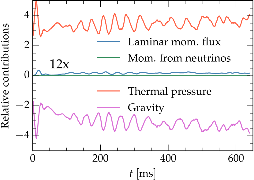
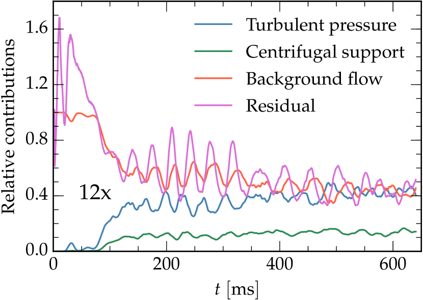
We show all terms of the RHS of Equation (54) for the 12x run in Figure 10. All of the terms are normalized by the sum of all terms, $\mathcal{F}$. For the purpose of making the figure easier to read, we separate these terms into two groups: terms associated with the “background” flow, shown in the left panel of the figure, and terms associated with the turbulent motion of the fluid, shown in the right panel.

Thermal pressure and gravity are the two largest terms in magnitude in Equation (54). The laminar part of the momentum flux (Equation 45) gives only a minor contribution and momentum deposition by neutrinos (Equation 48) is unsurprisingly negligible. Note that this does not mean that neutrino heating is negligible, but only that the direct deposition of momentum by neutrinos is small. The fact that thermal pressure term dominates in Figure 10 is not in contrast with what we find for the ratio of turbulent pressure to thermal pressure (Figure 7). Namely that turbulent pressure contributes significantly to the pressure balance. The reason for this apparent discrepancy is that most of the pressure support to the flow in Equation (46) comes from the bottom of the gain region, where turbulent pressure is only $\sim 5\%$ of the thermal pressure.

One of the first things that one notes from Figure 10 is that pressure and gravity nearly cancel each other. This means that, as a very first approximation, the flow can be considered to be quasi-stationary. The cancellation between pressure and gravity is, however, far from being exact, as can be seen from the red graph in the right panel of Figure 10, which summarizes the net effect of all background flow terms. This implies that, although the background flow is quasi-stationary, it is not static, but undergoes a secular evolution (mainly driven by the accumulation of mass and energy in the gain region; Section 3). The presence of secular changes in the flow is confirmed by the fact that $\mathcal{R}(t)$, which measures the rate of change of the total momentum of the flow, always has a positive sign and oscillates around a constant value for most of the simulation.

Turbulent convection can be seen as a perturbation on top of this slowly evolving background. The amplitude of the terms associated with turbulence in the right panel of Figure 10 is small if compared to that of those associated with gravity and thermal pressure. This means that the turbulent eddies are not strong enough to drastically alter the overall settling of the accretion flow. However, turbulent fluctuations are rather large on the scale associated with that of the secular changes of the accretion flow, as can be seen from the fact that turbulence terms in the right panel of Figure 10 are as large as the residual or the net background flow.

This is not too surprising in the light of our discussion in Section 4 on the energy and momentum equations. There we showed that turbulence produces large scale changes in the energy and momentum fluxes in space and time, but that the advection flow still dominates the overall energetics of the flow. Figure 10 provides a more quantitative and well defined way to measure this contribution.

Finally, it is worth pointing out that centrifugal support from non-radial motion produced by turbulence also provides a significant contribution to the dynamics of the flow. It provides of order $\sim 25\%$ of the turbulent pressure support. This is a factor that has been neglected in previous studies.

5.2. A Model for the Shock Evolution

So far, we have constructed a formal equation for the shock radius Equation (54) via momentum conservation. Then, we used this equation as a way to measure the relative importance of different terms in giving support to the shock. The following question arises naturally: is the equation we are using merely a trivial identity involving the shock radius? Or do the quantities $\mathcal{F}$, $\mathcal{R}$ and $r_{s}$ have deeper connections? Clearly, in the first case the analysis presented above would be of little value. The results of our simulations suggest that this is not the case and that $\mathcal{F}$ and $\mathcal{R}$ are relevant quantities determining the evolution of $r_{s}$.

In particular, we find that, given $\mathcal{F}$, $\mathcal{R}$, and the shock radius at a given time, it is possible to predict $r_{s,\mathrm{avg}}$ over a fraction of the advection timescale $\simeq 0.3\tau_{\mathrm{adv}}$ (Equation 14) with reasonable accuracy using a simple linear model based on Equation (54)

$$\left[\frac{r_{s,\mathrm{avg}}(t+0.3\tau_{\mathrm{adv}})}{1\ \mathrm{km}}\right]^{1/2}=A+B\mathcal{F}(t)+C\mathcal{R}(t)\,,$$ (55)

where $A$, $B$ and $C$ are coefficients that we fit using a least-squares procedure. For the 12x model, we find $A\simeq 4.84$, $B\simeq 8.54\times 10^{-44}\,\mathrm{s}^{2}\ \mathrm{g}^{-1}$ and $C\simeq 1.60\times 10^{-43}\,\mathrm{s}^{2}\ \mathrm{g}^{-1}$. We find similar values also for the other resolutions. However, we do not expect these values to be in any way universal. Actually, we find them to change by factors of order of a few when varying the heating factor $f_{\mathrm{heat}}$ in Equation (7). More on this below. Finally, we note that it is also possible to construct a similar model for $r_{s,\max}$. We focus on $r_{s,\mathrm{avg}}$ because its time evolution is smoother, while $r_{s,\max}$ necessarily “jumps” in steps that are multiple of the grid spacing, since our analysis is not able to identify the location of the shock to better than a single cell.

Figure 11.— Average shock radius evolution from the 12x run ($f_{\mathrm{heat}}=1.0$) at the retarded time $t+0.3\tau_{\mathrm{adv}}$ and its predicted value from the shock evolution Equation (55). For comparison we also show the average shock radius at the time when the prediction is made. The average shock radius can be accurately predicted over a fraction of the advection timescale (Equation 14) from the knowledge of $\mathcal{F}$ (Equation 51) and $\mathcal{R}$ (Equation 52).

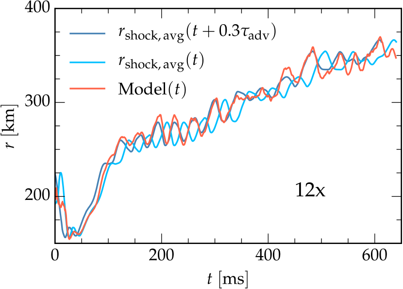
The results obtained with this simple model for the shock radius are shown in Figure 11. There, we show the prediction for the average shock radius at time $t+0.3\tau_{\mathrm{adv}}$ computed using the data available at time $t$, $\mathrm{Model}(t)$, the actual value of the average shock radius at the retarded time, $r_{s,\mathrm{avg}}(t+0.3\tau_{\mathrm{adv}})$, and the average shock radius at the time when the prediction is made, $r_{s,\mathrm{avg}}(t)$. As can be seen from the figure, the model specified by Equation (55) is able to predict both the shock radius oscillations and the secular trend of the shock radius with high accuracy. Note that we did not include any explicit term to model this trend in our fit: the entire shock evolution is contained in $\mathcal{F}$ and $\mathcal{R}$.

It is important to stress the fact that $\mathcal{F}$ and $\mathcal{R}$ encode information concerning the current shock position, as well as the flow in the gain region at the time when they are computed. They cannot be computed without resorting to a fully non-linear simulation. In this sense, Equation (55) is not predictive. The intriguing aspect of Equation (55) is that it suggests that $\mathcal{F}$ and $\mathcal{R}$ also encode information concerning the future shock position in a form which is easily extracted. This provides a validation to our interpretation of the different components of $\mathcal{F}$ and of their role in shaping the shock evolution (Section 5.1).

It is interesting to consider whether our simple model is able to predict the onset of a runaway explosion. This is difficult to fully assess with our simplified simulations, because we neglect important effects leading to the explosion, such as the sudden drop in the accretion rate following the accretion of the $\mathrm{Si/Si\,O}$ interface (Buras et al., 2006; Mezzacappa et al., 2007; Ugliano et al., 2012) or asphericities in the accretion flow (Couch & Ott 2013; Müller & Janka 2015). We also neglect the feedback of accretion on the neutrino luminosity and we do not include all of the necessary microphysics for a fully quantitative study.

Figure 12.— Shock radius at the retarded time $t+0.3\tau_{\mathrm{adv}}$ (dots) and its predicted value from the shock evolution (Equation 55) (solid lines) for the reference resolution, but using different heating factors.

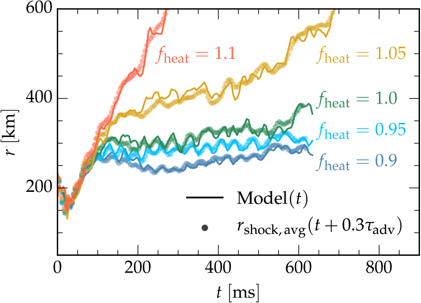
As a first step to study the reliability of our model for exploding simulations, we carry out a preliminary study were we obtain shock expansion / contraction by changing the value of $f_{\mathrm{heat}}$ in Equation (7) and fit the resulting shock evolutions using Equation (55). We perform these simulations at the reference resolution. As anticipated above, the fitting coefficients vary across the different runs. Nevertheless, we find Equation (55) to be well verified by all simulations. We show the results of this analysis in Figure 12.

As can be seen from this figure, the agreement between the predicted shock radius evolution from Equation (55) and the retarded average shock radius is reasonably good even as the heating factor is changed to the point that the model is starting to explode. The agreement is not as good as for the 12x model, possibly due to the higher numerical noise present in the reference resolution data in the cooling layer and in the first few grid points at the base of the gain region, where density and pressure increase steeply. This noise can contaminate $\mathcal{F}$ and $\mathcal{R}$ which are the two building blocks of Equation (55).

6. Turbulent Cascade

Following, e.g., Hanke et al. (2012); Couch (2013); Dolence et al. (2013); Couch & O’Connor (2014); Couch & Ott (2015) and Abdikamalov et al. (2015), we consider the power spectrum of the turbulent velocity $\delta\upsilon^{i}$ (Equation 28). Differently from most previous studies, however, we do not consider the spherical harmonics decomposition of the turbulent velocity on a sphere, but study the actual 3D spectrum of the turbulence.

During the evolution, at each time starting from $t\simeq 192\ \mathrm{ms}$ ($320\ \mathrm{ms}$ for the 20x resolution), we restrict our attention to the largest cubic region, $B$, entirely contained in the convectively unstable gain region and interpolate the turbulent velocity from the spherical grid used in our simulations to a uniform Cartesian grid defined on this region. Then, we compute the specific turbulent energy spectrum as the Fourier transform of the two-point correlation function

$$\tilde{E}(k)=\frac{1}{2}\int_{\mathbb{R}^{3}}\delta(|\mathbf{k}|-k)\widehat{\delta\upsilon_{i}^{*}}(\mathbf{k})\widehat{\delta\upsilon^{i}}(\mathbf{k})\mathrm{d}\mathbf{k}\,,$$ (56)

where $\delta(\cdot)$ is the Dirac delta, $\cdot^{*}$ denotes the complex conjugation and $\widehat{\delta\upsilon^{i}}$ is computed as

$$\widehat{\delta\upsilon^{i}}(\mathbf{k})=\int_{B}W(\mathbf{x})\delta\upsilon^{i}(\mathbf{x})\exp\left(2\pi\mathrm{i}\mathbf{k}\cdot\frac{\mathbf{x}}{L}\right)\mathrm{d}\mathbf{x}\,.$$ (57)

$W$ is a windowing function that smoothly goes to zero at the boundary of the box (more on this later), $L$ is the box size, and we neglected general-relativistic corrections in computing $\widehat{\delta\upsilon_{i}^{*}}$. Finally, in order to account for secular oscillations in the total turbulent energy, we normalize the spectrum to have unit integral

$$E(k)=\left[\int_{0}^{\infty}\tilde{E}(k)\mathrm{d}k\right]^{-1}\tilde{E}(k)\,,$$ (58)

and we average in time.

Windowing in the definition of the Fourier transform (57) is required because our data is not periodic. In particular, $W(\mathbf{x})$ is computed as

$$W(\mathbf{x})=W\left(\frac{x-x_{0}}{x_{1}-x_{0}}\right)W\left(\frac{y-y_{0}}{y_{1}-y_{0}}\right)W\left(\frac{z-z_{0}}{z_{1}-z_{0}}\right)\,,$$ (59)

where the $(x_{0},y_{0},z_{0})/(x_{1},y_{1},z_{1})$ are the minimum/maximum values of, respectively, $x,y$ and $z$ in the cube where we compute the spectra,

$$W(x)=\begin{cases}\exp\left[\frac{-1}{1-\left(\frac{x-\Delta}{\Delta}\right)^{2}}\right]&\textrm{if }x<\Delta\,,\\ 1&\textrm{if }\Delta\leq x\leq 1-\Delta\,,\\ \exp\left[\frac{-1}{1-\left(\frac{x-(1-\Delta)}{\Delta}\right)^{2}}\right]&\textrm{if }x>1-\Delta\,,\\ 0&\textrm{otherwise}\,,\end{cases}$$ (60)

and $\Delta$ is the grid spacing for the Cartesian grid, which we take to be equal to $\Delta r$.

Figure 13.— Compensated (i.e. multiplied by $k^{5/3}$) (right panel) and un-compensated (left-panel) specific turbulent energy power spectra, computed as in Equations (56) and (58) for the runs with $f_{\mathrm{heat}}=1.0$. The width of the shaded area around each curve represents the standard deviation of the energy spectrum during the averaging time window. The time average is done from $t\simeq 192\ \mathrm{ms}$ ($320\ \mathrm{ms}$ for the 20x resolution) until the end of the simulation.

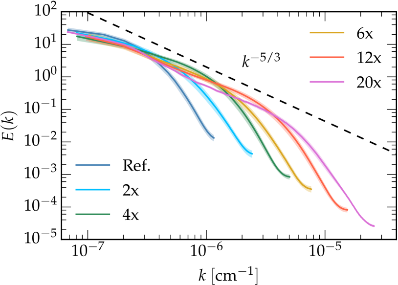
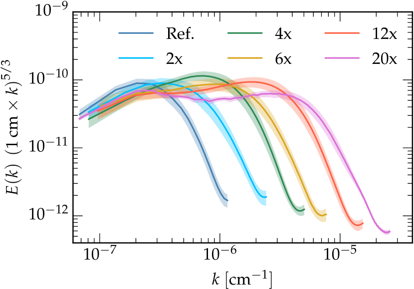
The normalized specific turbulent energy spectrum is shown in the left panel of Figure 13 for various resolutions. The right panel shows the spectra compensated (i.e. multiplied) by $k^{5/3}$ to highlight regions with Kolmogorov scaling, which we could expect on the basis of previous high-resolution local simulations (Radice et al., 2015). The shaded regions around each spectrum denote the standard deviation of the spectrum during the time-average window.

The slope of the spectra of low resolution simulations is rather shallow and consistent with a $k^{-1}$ scaling. The low resolution spectra are comparable to the ones reported at low-resolution by previous studies (Dolence et al., 2013; Couch & O’Connor, 2014; Couch & Ott, 2015; Abdikamalov et al., 2015). As argued by, Abdikamalov et al. (2015) and Radice et al. (2015), the $k^{-1}$ slope is due to the bottleneck effect artificially trapping turbulent energy at large scale.

As the resolution increases, the spectra become progressively steeper, but even the 12x resolution still shows a shallow $-4/3$ slope, indicative of the fact that even at this resolution the turbulence cascade is probably dominated by the bottleneck effect. However, the 20x resolution, which has over $1100$ points covering the gain region in the radial direction ($\sim 15$ times more than previous high-resolution simulations; Abdikamalov et al. 2015), finally shows an extended region compatible with the $k^{-5/3}$ scaling of Kolmogorov’s theory. This is particularly evident in the right panel of Figure 13 where we show the compensated spectrum.

This shows unambiguously that the shallow slopes reported in the CCSN literature are a finite-resolution effect, as previously argued by Abdikamalov et al. (2015) and Radice et al. (2015). It also give credence to the idea that the turbulent cascade of kinetic energy in neutrino-driven convection is well described by Kolmogorov theory, despite the presence of non-classical effects such as anisotropy, the geometric convergence of the flow, and mild compressibility.

Unfortunately, the computational costs of running at the 20x resolution are prohibitive even for our simplified setup and we could not run the 20x simulation for more than $\simeq 60\ \mathrm{ms}$, which is roughly equal to $\tau_{\mathrm{adv}}$. This is enough to study the energy spectrum at intermediate and small scales (including the inertial range), which we find to have reached a new equilibrium already $\sim 3\ \mathrm{ms}$ after the mapping from the 12x run. It is also sufficient to serve as benchmark data for future validation of turbulence models. Generating such benchmark data is one of the goals of the present work. It is not enough evolution time, however, to assess whether the structure of the gain layer and the general dynamics of the CCSN simulation model changes once the inertial range starts to be resolved.

7. Conclusions

Multi-dimensional instabilities are expected to play a fundamental role in the mechanism powering most CCSNe (e.g., Murphy & Meakin 2011; Murphy et al. 2013; Hanke et al. 2013; Couch 2013; Takiwaki et al. 2014; Couch & Ott 2015; Melson et al. 2015b; Lentz et al. 2015; Melson et al. 2015a). Neutrino-driven convection, in particular, is most commonly associated with post-collapse evolutions having strong neutrino heating and, in general, conditions that are most favorable for explosion (Dolence et al., 2013; Murphy et al., 2013; Ott et al., 2013; Couch, 2013; Couch & O’Connor, 2014; Takiwaki et al., 2014; Abdikamalov et al., 2015), however it is not excluded that SASI dominated CCSNe could also explode (Hanke et al., 2013; Fernández, 2015; Cardall & Budiardja, 2015).

Despite its central role in the context of the delayed neutrino mechanism, neutrino-driven convection has not been studied in a systematic way before. Previous studies were either performed in 2D, e.g., (Murphy & Meakin, 2011; Fernández et al., 2014), or spanned a relatively small range in resolution (Hanke et al., 2012; Dolence et al., 2013; Couch & O’Connor, 2014; Couch & Ott, 2015). Hence, it is difficult to assess to what level they are affected by finite-resolution effects. Abdikamalov et al. (2015) and Radice et al. (2015) showed that, at the resolutions typically used in 3D CCSN simulations the dynamics of the turbulent cascade of energy from large to small scale is severely affected by numerical viscosity. This artificially prevents kinetic energy from decaying to small scales and leads to an unphysical accumulation of energy at the largest scales, a phenomenon known as the bottleneck effect (Yakhot & Zakharov, 1993; She & Jackson, 1993; Falkovich, 1994; Verma & Donzis, 2007; Frisch et al., 2008). This large scale energy, in turn, results in an additional pressure support to the accreting flow (Radice et al., 2015). Considering the fact that turbulent pressure was found to be crucial in triggering explosions (Couch & Ott, 2015), having artificially large turbulent pressures, might result in a qualitative change in the evolution of a simulation. For this reason, it is important to quantify finite-resolution effects in CCSN simulations.

In the present study, we performed a series of semi-global neutrino-driven convection simulations with the goal of understanding the dynamics of neutrino-driven convection and the effects of finite resolution in CCSN simulations. Our simulations are rather unsophisticated when compared to state-of-the-art radiation-hydrodynamics simulations, e.g., (Melson et al., 2015a; Lentz et al., 2015). However, they include most of the basic physics ingredients relevant for neutrino-driven turbulent convection and they have the advantage of being completely under control. The converging geometry, the advection of gas through an accretion shock toward a central PNS, gravity, photo-dissociation of heavy-nuclei at the shock and neutrino/heating cooling are all included in a completely controlled way. The main limitations of our model are that we neglect the non-linear feedback between accretion and neutrino luminosity, which we assume to be constant, and that we fix the amount of specific energy lost to nuclear dissociation. These approximations would be particularly limiting in the study of the transition to explosion of our models. Such a study would require us to follow the shock as it develops large radial displacements with respect to its initial conditions and correctly account for significant changes in the accretion rate. However, this is not the aim of this work. Our current approximations are expected to be adequate for the study of the nearly stationary neutrino-driven convection we report here. We considered a constant accretion rate and analytic, stationary initial conditions so as to be able to perform long term evolutions and collect well-resolved statistics of the turbulent flow. We employed high-order, low dissipation numerical methods, a grid adapted to the problem (a spherical wedge) and we varied the grid scaling across different simulations by a factor 20, achieving unprecedented resolutions for this kind of study, with a radial spacing of $191\ \mathrm{m}$ and an angular resolution of $0.09^{\circ}$ in the gain layer.

We find that, as resolution increases, the qualitative dynamics of the flow changes drastically. At low resolution, the dynamics is characterized by the presence of large, slowly evolving, high-entropy plumes. At higher resolution, the dynamics is dominated by smaller structures evolving on a faster timescale. Given that the transition to explosion seems to be preceded by the formation of large, long-lived, high-entropy plumes (Fernández et al., 2014; Müller & Janka, 2015; Lentz et al., 2015), this is a first indication that low resolution might be artificially favouring explosion.

At high resolution, turbulent mixing is very effective at smoothing out sharp interfaces between high and low entropy regions: high-entropy plumes lose their coherence due to small scale mixing and they resemble more “clouds” than “bubbles”. This means that the separation of the flow into very well defined high and low entropy regions seen in most simulations is also an artifact of low resolution. This is not too surprising: the physics of neutrino-driven convection is not that of a multiphase flow. This calls into question the usefulness of arguments describing neutrino-driven convection in terms of an ensemble of “bubbles” moving through the accretion flow.

Despite these large qualitative changes with resolution, but as predicted by Radice et al. (2015), we find large scale quantities to be consistent among the different resolutions for our fiducial model. In other words, we find global quantities, such as the shock radius, the typical timescales for advection and heating, to be consistent across all of the resolutions and to be even monotonically convergent in the first $100\ \mathrm{ms}$, a phase in which convection is developing, but the buoyant plumes have not yet managed to strongly interact with the shock. Note, however, that we also find that this picture changes drastically for models where we induce an expansion of the shock by artificially increasing the heating rate. For these models, we find low and high resolution simulation to be diverging after the first $50\ \mathrm{ms}$ and low resolution simulations showing earlier shock expansion.

We also find, in agreement with Hanke et al. (2012) and Abdikamalov et al. (2015), that low resolution typically yields more favorable conditions for explosion, especially at early times. These differences are rather modest for our fiducial set of simulations, but are more pronounced for simulations that are closer to or at the transition to explosion. Given that some of the current full-physics models appear to be on the verge of explosion (Melson et al., 2015a), our results serve as an additional reminder that a resolution study is necessary to confirm any result. At the same time, we think, in the light of our findings, that some cautious optimism can be justified in the sense that many quantities of interest in CCSNe appear to be well converged at modest resolution, even though others, like the velocity spectra $E(k)$, are affected by serious artifacts until very high resolution is reached.

Furthermore, it is interesting to note that our results suggest that the flow dynamics and the resulting CCSN evolution may change quantitatively and qualitatively at very high resolution when turbulence begins to be resolved. The simulation at twelve times our fiducial resolution exhibits a reversal of the just discussed trend with resolution: its shock radius evolution has the steepest slope. Explosion diagnostics such as the ratio of advection to heating timescales suggest that it is approaching explosion faster than less resolved simulations. We cannot fully understand this trend until it becomes possible to carry out even higher-resolution long-term simulations. However, we speculate that our finding may be a consequence of the increasing non-linear coupling of a greater range of scales and the development of strong intermittency as the inertial range of turbulence begins to be resolved. The effects of fully resolved turbulence (perhaps captured by a sub-grid model) may ultimately be beneficial for explosion.

In order to better quantify the importance of turbulent convection for CCSN explosions, we studied the efficiency with which neutrino-driven convection transports energy and momentum across the gain region. We find the energy balance in the flow to be dominated by the thermal energy and the overall energetics to be driven by the background advective flow. Turbulence opposes the overall negative (down-flowing) radial enthalpy fluxes, but it is only able to contribute a small $\sim 10\%$ correction to the overall thermal energy flow. The kinetic energy evolution, on the other hand, is dominated by turbulence, which provides $\sim 80\%$ of the kinetic energy flux and $\sim 90\%$ of the advective part of the momentum flux (the part of the momentum flux not containing the pressure gradient). We also find the effective pressure support provided by turbulence to be significant and of the order of $\sim 30\%-40\%$ of the thermal pressure in our simulations.

According to our results neutrino-driven turbulent convection plays a more important role in the evolution of the momentum than in the evolution of the energy. This suggest that the large differences in, e.g., shock radii, between turbulent multi-dimensional and one-dimensional simulations can be mostly accounted for by the effects of turbulence in the momentum equation in agreement with Couch & Ott (2015). In this respect, we showed that it is possible to derive an equation that can explain and even predict the shock radius evolution over a fraction of the advection timescale starting from integrals of the terms appearing in the radial momentum equation. This new diagnostic generalizes and refines the approach by Murphy et al. (2013) in which the shock position was derived starting from an approximated angle-averaged shock jump condition. With our approach it is possible to quantify, in a rigorous way, the relative importance of different terms in providing pressure support to the shock. Our analysis suggests that turbulence plays an indirect role in the revival of the shock. Rather than directly transporting energy to the shock, turbulence acts as an effective barrier slowing down the drain of energy from the shock by the radial advection.

We studied the turbulent energy cascade in the gain region by means of the 3D power-spectrum of the turbulent velocity $E(k)$. We find conclusive evidence that the shallow spectra reported by many investigations are the result of the numerical bottleneck effect, as previously suggested by Abdikamalov et al. (2015). In particular, we observe that as resolution increases, the spectra become progressively steeper. At the highest resolution, the spectrum has a slope compatible with the $k^{-5/3}$ slope predicted by the classical theory of Kolmogorov, e.g., Pope (2000), and as suggested by local simulations (Radice et al., 2015).

Unfortunately, resolving the inertial range of neutrino-driven convection requires resolutions that are not even affordable for a full simulation in our simplified setup and that could only be employed to simulate a relatively short time frame ($\simeq 60\ \mathrm{ms}$) starting from a lower resolution simulation. This was enough to be able to measure the spectrum of the turbulent kinetic energy, which we find to have already reached a new equilibrium after $\sim 3\ \mathrm{ms}$. However, these $60\ \mathrm{ms}$ of evolution are not enough to fully assess the ramifications of not resolving the inertial range in a global simulation. Our simulations appear to be already converged at large scale, but the difference between resolving and not resolving the inertial range could become more substantial for models close to the explosion threshold.

At the moment, achieving a resolution sufficient to fully resolve the inertial range dynamics in global simulations seems to be impossible. At the same time, the numerical schemes currently adopted for CCSN simulations show rather poor performance for under-resolved turbulent flows (Radice et al., 2015). It is thus our opinion that performing qualitatively and quantitatively accurate CCSN simulations will require the use of some form of turbulent closure. In future work, we plan to use the simulation data presented here as a basis to guide the construction of numerical turbulent closures specialized for CCSN applications.

Appendix A A. Parametrized Nuclear Dissociation Treatment

Nuclear dissociation is included in a parametrized way using an approach similar to that of Fernández & Thompson (2009b, a), but with some important differences discussed here.

Fernández & Thompson (2009b) suggested to parametrize the amount of specific internal energy lost to nuclear dissociation, $\epsilon_{\mathrm{ND}}$, as a fraction, $\bar{\epsilon}$, of the free-fall kinetic energy at the initial location of the shock:

$$\epsilon_{\mathrm{ND}}=\frac{1}{2}\bar{\epsilon}\,\upsilon_{\mathrm{FF}}^{2}\,,$$ (A1)

where $\upsilon_{\mathrm{FF}}$ is the free-fall velocity at the initial location of the shock. In the relativistic case this translates to

$$\epsilon_{\mathrm{ND}}=\bar{\epsilon}(W_{\mathrm{FF}}-1)\,,$$ (A2)

where $W_{\mathrm{FF}}$ is the free-fall Lorentz factor (see Appendix B). A typical range of values for $\bar{\epsilon}$ is $0.2-0.4$ (Fernández & Thompson, 2009a).

Fernández & Thompson (2009b, a) used the nuclear burning module of the FLASH code Fryxell et al. (2000) to simulate nuclear dissociation with the inclusion of an energy sink term. This approach is perfectly viable in classical hydrodynamics, but not in the relativistic case, because, in relativistic hydrodynamics, the inertia (and momentum) of the fluid depends on the enthalpy and, for this reason, a sink term in the energy equation would result in an inconsistency with the shock jump conditions. In our implementation, instead, nuclear dissociation is included in the equation of state as follows. We model the effect of the thermal energy lost to nuclear dissociation with a modified gamma-law of the form

$$p=(\gamma-1)\rho\big{(}\epsilon-\epsilon_{\mathrm{ND}}^{\ast}(\epsilon)\big{)}\,,$$ (A3)

where

$$\epsilon^{\ast}_{\mathrm{ND}}(\epsilon)=\begin{cases}0\,,&\textrm{if }\epsilon\leq\epsilon_{\mathrm{ND}}\,,\\ \eta(\epsilon-\epsilon_{\mathrm{ND}})\,,&\textrm{if }\epsilon_{\mathrm{ND}}<\epsilon\leq\epsilon_{\mathrm{ND}}\big{(}\frac{\eta+1}{\eta}\big{)}\,,\\ \epsilon_{\mathrm{ND}}\,,&\textrm{if }\epsilon>\epsilon_{\mathrm{ND}}\big{(}\frac{\eta+1}{\eta}\big{)}\,,\end{cases}$$ (A4)

and $\eta=0.95$ is an efficiency parameter needed to ensure that $p(\rho,\cdot)$ is a one-to-one function (this is needed for the recovery of $\rho,\upsilon^{i}$ and $\epsilon$ from the evolved variables at the end of each iteration during the evolution). Another advantage of this approach, as compared to the one of Fernández & Thompson (2009b, a), is that it does not involve possibly stiff cooling terms that can give rise to numerical problems.

The results presented in this paper are obtained with $\bar{\epsilon}=0.3$, which corresponds to a value of $\epsilon_{\mathrm{ND}}=0.003$ ($\simeq 2.7\times 10^{18}\ \mathrm{erg}\ \mathrm{g}^{-1}$) for a shock stalled at $100$ Schwarzschild radii of the PNS ($\simeq 191\ \mathrm{km}$). We remark that our results are sensitive to the choice of $\bar{\epsilon}$, because the flow becomes stable against the development of convection when $\bar{\epsilon}$ is sufficiently small. The reason is that smaller $\bar{\epsilon}$ result in larger radial velocities immediately downstream from the shock, which, in turn, prevent buoyant instabilities from growing into fully-developed convection before being advected out of the gain region (Foglizzo et al., 2006). For more details, we refer to the studies of Fernández & Thompson (2009b, a), and Cardall & Budiardja (2015) that showed the impact of nuclear dissociation on the development of neutrino-driven convection and SASI.

Appendix B B. Relativistic Standing Accretion Shock Solution

The initial conditions of our simulations represent a stationary standing accretion shock. Our model is similar to the neutron star (NS) accretion models of Chevalier (1989); Houck & Chevalier (1992) and the CCSN model of Janka (2001), which has been used in many studies of SASI and convection, e.g., Blondin et al. (2003); Foglizzo et al. (2006); Cardall & Budiardja (2015).

To construct the initial conditions, we solve the equations of relativistic hydrodynamics (1) on top of a fixed gravitational background (Equation 5) time-independently. Heating, cooling and nuclear dissociation are also taken into account in the same way as for the subsequent numerical evolution. The initial conditions are specified by choosing values for the PNS radius, $r_{\mathrm{PNS}}$, the shock radius, $r_{s}$, the accretion rate $\dot{M}$, and the heating coefficient $K$. The heating/cooling normalization coefficient $C$ is then tuned so that the velocity vanishes at the PNS radius.

B.1. Pre-Shock Flow

The pre-shock flow is assumed to be cold and free falling, so that the pre-shock Lorentz factor $W_{0}$ can be computed from the lapse function at the location of the shock: $W_{0}=\frac{1}{\alpha_{0}}$. The pre-shock density is computed by fixing the accretion rate $\dot{M}$:

$$\rho_{0}=\frac{\dot{M}}{4\pi r_{s}^{2}W_{0}|\upsilon_{0}^{r}|}\,,$$ (B1)

where $\upsilon_{0}^{r}$ is the radial component of the pre-shock velocity. In practice, for numerical reasons, to minimize disturbances in the upstream flow, our initial conditions have a small, but non-zero, pre-shock internal energy $\epsilon_{0}$, which we compute from the requirement that the Mach number of the upstream flow should be equal to $100$.

B.2. Shock Jump Conditions

The post-shock density, pressure and velocity can be computed from the Rankine-Hugoniot conditions of a stationary shock

$$\rho_{1}W_{1}\upsilon_{1}^{r} =\rho_{0}W_{0}\upsilon_{0}^{r}\,,$$ (B2a)

$$\rho_{1}h_{1}W_{1}^{2}(\upsilon_{1}^{r})^{2}+p_{1}\alpha^{2} =\rho_{0}h_{0}W_{0}^{2}(\upsilon_{0}^{r})^{2}+p_{0}\alpha^{2}\,,$$ (B2b)

$$\rho_{1}h_{1}W_{1}^{2}\upsilon_{1}^{r} =\rho_{0}h_{0}W_{0}^{2}\upsilon_{0}^{r}\,,$$ (B2c)

where the indices $0$ and $1$ refer to pre- and post-shock quantities, respectively, and we made use of Equation (6). Note that the effect of dissociation is automatically included in these jump conditions, since it is accounted for in the equation of state.

In the strong shock limit, $\epsilon_{0}\ll 1$, and for small post-shock velocities, $W_{1}\simeq 1$, they can be simplified as

$$\rho_{1}\upsilon_{1}^{r} =\rho_{0}W_{0}\upsilon_{0}^{r}\,,$$ (B3a)

$$\rho_{1}h_{1}(\upsilon_{1}^{r})^{2}+p_{1}\alpha^{2} =\rho_{0}W_{0}^{2}(\upsilon_{0}^{r})^{2}\,,$$ (B3b)

$$\rho_{1}h_{1}\upsilon_{1}^{r} =\rho_{0}W_{0}^{2}\upsilon_{0}^{r}\,.$$ (B3c)

These can easily be solved for the post-shock density,

$$\rho_{1}=\rho_{0}W_{0}\frac{\upsilon_{0}^{r}}{\upsilon_{1}^{r}}\,,$$ (B4)

specific internal energy

$$\epsilon_{1}=\frac{W_{0}-1+(\gamma-1)\epsilon_{\mathrm{ND}}}{\gamma}\,,$$ (B5)

and velocity

$$\upsilon_{1}^{r}=\frac{\upsilon_{0}^{r}+\sqrt{(\upsilon_{0}^{r})^{2}-4\psi}}{2}\,,$$ (B6)

where

$$\psi=\alpha^{2}\frac{\gamma-1}{\gamma}\frac{W_{0}-1-\epsilon_{\mathrm{ND}}}{W_{0}}\,.$$ (B7)

Note that Equation (B5) is valid as long as $\bar{\epsilon}$ is sufficiently small so that

$$\bar{\epsilon}\bigg{(}\frac{\eta+1}{\eta}-\frac{\gamma-1}{\gamma}\bigg{)}\leq\frac{1}{\gamma}.$$ (B8)

For $\gamma=4/3$ and $\eta=0.95$ this means $\bar{\epsilon}\lesssim 0.42$, which is satisfied since we take $\bar{\epsilon}=0.3$.

B.3. Post-Shock Flow

The initial post-shock flow is computed by looking for a time-independent version of Equation (1), with boundary-conditions given by the post-shock density, velocity and specific internal energy. Note that, as we show later, the equations are singular at the point where $\upsilon^{r}=0$ and no boundary condition is required downstream of the shock. Instead, the normalization coefficient of the heating/cooling source, $S$, has to be adjusted so that $\upsilon^{r}$ vanishes at the surface of the PNS.

The first condition that we use is the continuity equation (first part of Equation 1), that, in the stationary, spherically symmetric case, is simply

$$r^{2}\rho W\upsilon^{r}=\frac{1}{4\pi}\dot{M}\,.$$ (B9)

The energy equation is rewritten in non-conservation form, by projecting the second part of Equation (1) along the velocity four-vector, to yield (see e.g., Gourgoulhon 2006 for a detailed derivation)

$$u^{\mu}\nabla_{\mu}(\rho\epsilon)=-(\rho\epsilon+p)\nabla_{\mu}u^{\mu}+\mathcal{L}\,.$$ (B10)

In the stationary, spherically symmetric case, this becomes

$$\frac{\dot{M}}{4\pi}\partial_{r}\epsilon=-2prW\upsilon^{r}-pr^{2}\partial_{r}(W\upsilon^{r})+\mathcal{L}\,.$$ (B11)

Similarly, the momentum equation is also rewritten in non-conservation form, by projecting the second part of Equation (1) perpendicularly to $u^{\mu}$ to obtain the relativistic Euler equations,

$$\rho ha_{\mu}=-\nabla_{\mu}p-u^{\nu}\nabla_{\nu}pu_{\mu}\,,$$ (B12)

where $a_{\mu}$ is the relativistic 4-acceleration vector

$$a_{\mu}=u^{\nu}\nabla_{\nu}u_{\mu}=u^{\nu}(\partial_{\nu}u_{\mu}-\Gamma^{\alpha}_{\phantom{\alpha}\nu\mu}u_{\alpha})\,,$$ (B13)

and $\Gamma^{\alpha}_{\phantom{\alpha}\nu\mu}$ are the Christoffel symbols of the Levi-Civita connection. In our case, the Euler equation reduces to

$$\rho hW\upsilon^{r}A^{2}\partial_{r}(W\upsilon^{r})=\frac{1}{A^{4}}\frac{2M}{r^{2}}\rho hW^{2}(\upsilon^{r})^{2}-\big{[}1+A^{2}W^{2}(\upsilon^{r})^{2}\big{]}\partial_{r}p-\frac{A^{2}}{r^{2}}MW^{2}\big{[}1+A^{2}(\upsilon^{r})^{2}\big{]}\rho h\,.$$ (B14)

Note that this equation has a manifest singularity for $\upsilon^{r}=0$. In practice, $\upsilon^{r}$ is never exactly equal to zero, although tuning $C$ yields very small values of $|\upsilon^{r}|$ close to the surface of the PNS, and we find that the ODE integrator of our choice, the implicit multistep “MSBDF” method implemented in the GNU Scientific Library (Galassi & Gough, 2009), is sufficiently robust to handle these equations.

Finally we can substitute the derivative of the pressure in the right-hand-side of Equation (B14) using the EOS to find

$$\begin{split}\Big{[}\rho hW\upsilon^{r}A^{2}-\frac{\gamma p}{W\upsilon}\big{(}1+A^{2}W^{2}(\upsilon^{r})^{2}\big{)}\Big{]}&\partial_{r}(W\upsilon^{r})=\\ &\frac{1}{A^{4}}\frac{2M}{r^{2}}\rho hW^{2}(\upsilon^{r})^{2}+\frac{1+A^{2}W^{2}(\upsilon^{r})^{2}}{r^{2}W\upsilon^{r}}\big{[}2\gamma rW\upsilon^{r}p-(\gamma-1)\mathcal{L}\big{]}-\frac{A^{2}}{r^{2}}MW^{2}\big{[}1+A^{2}(\upsilon^{r})^{2}\big{]}\rho h\,.\end{split}$$ (B15)

Figure 14.— Initial data profiles. Left panel: density and velocity. Right panel: entropy and Brunt-Väisäla frequency $\Omega_{\mathrm{BV}}$ computed as in Equations (4) and (12).

Equations (B9), (B11) and (B15) are the ones that we solve numerically, together with the EOS, to generate our initial conditions. Figure 14, shows the profile of the entropy and the Brunt-Väisäla frequency for the initial conditions used throughout this study.

References

- Abdikamalov et al. (2015) Abdikamalov, E., Ott, C. D., Radice, D., et al. 2015, ApJ, 808, 70
- Banyuls et al. (1997) Banyuls, F., Font, J. A., Ibáñez, J. M., Martí, J. M., & Miralles, J. A. 1997, ApJ, 476, 221
- Bethe (1990) Bethe, H. A. 1990, Rev. Mod. Phys., 62, 801
- Bethe & Wilson (1985) Bethe, H. A., & Wilson, J. R. 1985, ApJ, 295, 14
- Blondin & Mezzacappa (2007) Blondin, J. M., & Mezzacappa, A. 2007, Nature, 445, 58
- Blondin et al. (2003) Blondin, J. M., Mezzacappa, A., & DeMarino, C. 2003, ApJ, 584, 971
- Buras et al. (2006) Buras, R., Janka, H.-T., Rampp, M., & Kifonidis, K. 2006, A&A, 457, 281
- Burrows (2013) Burrows, A. 2013, Rev. Mod. Phys., 85, 245
- Burrows & Goshy (1993) Burrows, A., & Goshy, J. 1993, ApJ, 416, L75
- Burrows et al. (1995) Burrows, A., Hayes, J., & Fryxell, B. A. 1995, ApJ, 450, 830
- Cardall & Budiardja (2015) Cardall, C. Y., & Budiardja, R. D. 2015, ApJ, 813, L6
- Chevalier (1989) Chevalier, R. A. 1989, ApJ, 346, 847
- Couch (2013) Couch, S. M. 2013, ApJ, 775, 35
- Couch et al. (2015) Couch, S. M., Chatzopoulos, E., Arnett, W. D., & Timmes, F. X. 2015, ApJ, 808, L21
- Couch & O’Connor (2014) Couch, S. M., & O’Connor, E. P. 2014, ApJ, 785, 123
- Couch & Ott (2013) Couch, S. M., & Ott, C. D. 2013, ApJ, 778, L7
- Couch & Ott (2015) —. 2015, ApJ, 799, 5
- Dolence et al. (2013) Dolence, J. C., Burrows, A., Murphy, J. W., & Nordhaus, J. 2013, ApJ, 765, 110
- Endeve et al. (2012) Endeve, E., Cardall, C. Y., Budiardja, R. D., et al. 2012, ApJ, 751, 26
- Falkovich (1994) Falkovich, G. 1994, Phys. Fluids, 6, 1411
- Fernández (2012) Fernández, R. 2012, ApJ, 749, 142
- Fernández (2015) —. 2015, MNRAS, 452, 2071
- Fernández et al. (2014) Fernández, R., Müller, B., Foglizzo, T., & Janka, H.-T. 2014, MNRAS, 440, 2763
- Fernández & Thompson (2009a) Fernández, R., & Thompson, C. 2009a, ApJ, 703, 1464
- Fernández & Thompson (2009b) —. 2009b, ApJ, 697, 1827
- Foglizzo et al. (2007) Foglizzo, T., Galletti, P., Scheck, L., & Janka, H.-T. 2007, ApJ, 654, 1006
- Foglizzo et al. (2006) Foglizzo, T., Scheck, L., & Janka, H.-T. 2006, ApJ, 652, 1436
- Foglizzo et al. (2015) Foglizzo, T., Kazeroni, R., Guilet, J., et al. 2015, Pub. Ast. Soc. Aus., 32, e009
- Frisch et al. (2008) Frisch, U., Kurien, S., Pandit, R., et al. 2008, Phys. Rev. Lett., 101, 144501
- Fryxell et al. (2000) Fryxell, B., Olson, K., Ricker, P., et al. 2000, ApJS, 131, 273
- Gabay et al. (2015) Gabay, D., Balberg, S., & Keshet, U. 2015, ApJ, 815, 37
- Galassi & Gough (2009) Galassi, M., & Gough, B. 2009, GNU Scientific Library: Reference Manual, GNU manual (Network Theory)
- Gourgoulhon (2006) Gourgoulhon, E. 2006, 37
- Handy et al. (2014) Handy, T., Plewa, T., & Odrzywołek, A. 2014, ApJ, 783, 125
- Hanke et al. (2012) Hanke, F., Marek, A., Müller, B., & Janka, H.-T. 2012, ApJ, 755, 138
- Hanke et al. (2013) Hanke, F., Müller, B., Wongwathanarat, A., Marek, A., & Janka, H.-T. 2013, ApJ, 770, 66
- Herant (1995) Herant, M. 1995, Phys. Rep., 256, 117
- Houck & Chevalier (1992) Houck, J. C., & Chevalier, R. A. 1992, ApJ, 395, 592
- Janka (2001) Janka, H.-T. 2001, A&A, 368, 527
- Janka et al. (2012) Janka, H.-T., Hanke, F., Hüdepohl, L., et al. 2012, Prog. Th. Exp. Phys., 2012, 010000
- Janka et al. (2007) Janka, H.-T., Langanke, K., Marek, A., Martínez-Pinedo, G., & Müller, B. 2007, Phys. Rep., 442, 38
- Janka & Müller (1996) Janka, H.-T., & Müller, E. 1996, A&A, 306, 167
- Lentz et al. (2015) Lentz, E. J., Bruenn, S. W., Hix, W. R., et al. 2015, ApJ, 807, L31
- Liebendörfer et al. (2001) Liebendörfer, M., Mezzacappa, A., Thielemann, F.-K., et al. 2001, Phys. Rev. D, 63, 103004
- Liebendörfer et al. (2005) Liebendörfer, M., Rampp, M., Janka, H.-T., & Mezzacappa, A. 2005, ApJ, 620, 840
- Marek & Janka (2009) Marek, A., & Janka, H.-T. 2009, ApJ, 694, 664
- Meakin & Arnett (2007) Meakin, C. A., & Arnett, D. 2007, ApJ, 667, 448
- Melson et al. (2015a) Melson, T., Janka, H.-T., Bollig, R., et al. 2015a, ApJ, 808, L42
- Melson et al. (2015b) Melson, T., Janka, H.-T., & Marek, A. 2015b, ApJ, 801, L24
- Mezzacappa et al. (2007) Mezzacappa, A., Bruenn, S. W., Blondin, J. M., Hix, W. R., & Bronson Messer, O. E. 2007, in AIP Conf. Ser., Vol. 924, The Multicolored Landscape of Compact Objects and Their Explosive Origins, ed. T. di Salvo, G. L. Israel, L. Piersant, L. Burderi, G. Matt, A. Tornambe, & M. T. Menna, 234
- Müller & Janka (2015) Müller, B., & Janka, H.-T. 2015, MNRAS, 448, 2141
- Müller et al. (2012) Müller, B., Janka, H.-T., & Marek, A. 2012, ApJ, 756, 84
- Murphy & Burrows (2008) Murphy, J. W., & Burrows, A. 2008, ApJ, 688, 1159
- Murphy & Dolence (2015) Murphy, J. W., & Dolence, J. C. 2015, ArXiv:1507.08314
- Murphy et al. (2013) Murphy, J. W., Dolence, J. C., & Burrows, A. 2013, ApJ, 771, 52
- Murphy & Meakin (2011) Murphy, J. W., & Meakin, C. 2011, ApJ, 742, 74
- Ott et al. (2013) Ott, C. D., Abdikamalov, E., Mösta, P., et al. 2013, ApJ, 768, 115
- Pejcha & Thompson (2012) Pejcha, O., & Thompson, T. A. 2012, ApJ, 746, 106
- Pope (2000) Pope, S. B. 2000, Turbulent Flows, ed. Pope, S. B. (Cambridge Univ. Press, Cambridge, UK)
- Radice et al. (2015) Radice, D., Couch, S. M., & Ott, C. D. 2015, CompAC, 2
- Radice & Rezzolla (2012) Radice, D., & Rezzolla, L. 2012, A&A, 547, A26
- Radice et al. (2014) Radice, D., Rezzolla, L., & Galeazzi, F. 2014, Class. Quantum Grav., 31, 075012
- Rampp & Janka (2000) Rampp, M., & Janka, H.-T. 2000, ApJ, 539, L33
- She & Jackson (1993) She, Z., & Jackson, E. 1993, Phys. Fluids, 5, 1526
- Sumiyoshi et al. (2005) Sumiyoshi, K., Yamada, S., Suzuki, H., et al. 2005, ApJ, 629, 922
- Suresh & Huynh (1997) Suresh, A., & Huynh, H. T. 1997, J. Comp. Phys., 136, 83
- Takiwaki et al. (2012) Takiwaki, T., Kotake, K., & Suwa, Y. 2012, ApJ, 749, 98
- Takiwaki et al. (2014) —. 2014, ApJ, 786, 83
- Thompson et al. (2003) Thompson, T. A., Burrows, A., & Pinto, P. A. 2003, ApJ, 592, 434
- Ugliano et al. (2012) Ugliano, M., Janka, H.-T., Marek, A., & Arcones, A. 2012, ApJ, 757, 69
- Verma & Donzis (2007) Verma, M. K., & Donzis, D. 2007, J. Phys. A, 40, 4401
- Yakhot & Zakharov (1993) Yakhot, V., & Zakharov, V. 1993, Phys. D, 64, 379
- Yamasaki & Yamada (2006) Yamasaki, T., & Yamada, S. 2006, ApJ, 650, 291