Non-Hermitian Dynamics in the Quantum Zeno Limit

Abstract

We show that weak measurement leads to unconventional quantum Zeno dynamics with Raman-like transitions via virtual states outside the Zeno subspace. We extend this concept into the realm of non-Hermitian dynamics by showing that the stochastic competition between measurement and a system’s own dynamics can be described by a non-Hermitian Hamiltonian. We obtain a solution for ultracold bosons in a lattice and show that a dark state of tunnelling is achieved as a steady state in which the observable’s fluctuations are zero and tunnelling is suppressed by destructive matter-wave interference.

I Introduction

Frequent measurements can slow the evolution of a quantum system leading to the quantum Zeno effect Misra and Sudarshan (1977); Facchi and Pascazio (2008) which has been successfully observed in a variety of systems Itano et al. (1990); Nagels et al. (1997); Kwiat et al. (1999); Balzer et al. (2000); Streed et al. (2006); Hosten et al. (2006); Bernu et al. (2008). One can also devise measurements with multi-dimensional projections which lead to quantum Zeno dynamics where unitary evolution is uninhibited within this degenerate subspace, i.e. the Zeno subspace Facchi and Pascazio (2008); Raimond et al. (2010, 2012); Signoles et al. (2014). In this paper we go beyond conventional quantum Zeno dynamics. By considering the case of measurement near, but not in, the projective limit the system is still confined to a Zeno subspace, but intermediate transitions are allowed via virtual Raman-like processes. We show that this can be approximated by a non-Hermitian Hamiltonian thus extending the notion of quantum Zeno dynamics into the realm of non-Hermitian quantum mechanics joining the two paradigms.

Non-Hermitian systems exhibit a variety of rich behaviour, such as localisation Hatano and Nelson (1996); Refael et al. (2006), $\mathcal{PT}$ symmetry Bender and Boettcher (1998); Giorgi (2010); Zhang and Song (2013), spatial order Otterbach and Lemeshko (2014), or novel phase transitions Lee and Chan (2014); Lee et al. (2014). Recent experimental results further motivate the study of these novel phenomena Dembowski et al. (2001); Choi et al. (2010); Ruter et al. (2010); Barontini et al. (2013); Gao et al. (2015). Non-Hermitian Hamiltonians commonly arise in systems with decay or loss Dhar et al. (2015); Stannigel et al. (2014), limited by possibilities of controlling dissipation. Additionally, the non-unitary time evolution is subject to discontinuous jumps applied whenever decay events are detected requiring the postselection of trajectories Otterbach and Lemeshko (2014); Lee and Chan (2014); Lee et al. (2014). Here we consider systems where the non-Hermitian term arises from measurement and uncover a novel general mechanism that is independent of the nature of the original Hamiltonian. It does not rely on losses or postselection of exotic trajectories, thus conceptually simplifying experimental realizability of such intriguing effects. Furthermore, we show that the physics can be much more complicated and lead to dynamics beyond the conventional Hermitian and quantum Zeno dynamics paradigms.

As an example, we demonstrate the effects of non-Hermitian evolution by investigating a gas of ultracold bosons in a lattice inside an optical cavity which are subjects of intensive interdisciplinary research Bloch et al. (2007); Lewenstein et al. (2007); Ritsch et al. (2013); Mekhov and Ritsch (2012). This field is extremely flexible when it comes to engineering measurement Ruostekoski and Walls (1997); Mekhov et al. (2007a); Chen and Meystre (2009); Mekhov and Ritsch (2009a, 2010, 2011, 2012); Mekhov (2013); Pedersen et al. (2014); Elliott et al. (2015a); Kozlowski et al. (2015); Mazzucchi et al. (2016a); Elliott et al. (2015b); Wade et al. (2015); Ashida and Ueda (2015); Mazzucchi et al. (2016b); Caballero-Benitez et al. (2016). Furthermore, it is a realistic experimental proposal for our theoretical model given the rapid progress in merging quantum optics with ultracold gases Baumann et al. (2010); Wolke et al. (2012); Schmidt et al. (2014); Miyake et al. (2011); Weitenberg et al. (2011) including the most recent realizations of an optical lattice in a high-Q cavity Landig et al. (2016); Klinder et al. (2015). We go beyond quantum nondemolition approaches where the measurement backaction or many-body dynamics were neglected Mekhov et al. (2007b, c); Eckert et al. (2008); Roscilde et al. (2009); Mekhov and Ritsch (2009b, c); De Chiara et al. (2011); Hauke et al. (2013); Rogers et al. (2014). We will show that, counter-intuitively, non-Hermitian dynamics causes two competing processes, tunnelling and measurement, to cooperate to form a dark state of the atomic dynamics with zero fluctuations in the observed quantity without the need for an effective cavity potential which is typically considered in self-organisation Nagy et al. (2008); Niedenzu et al. (2013); Bakhtiari et al. (2015); Ivanov and Ivanova (2015); Schütz et al. (2015); Winterauer et al. (2015); Piazza and Ritsch (2015).

II Theoretical Model - Measurement Induced Non-Hermitian Dynamics

II.1 Suppression of Coherences in the Density Matrix by Strong Measurment

We consider a state described by the density matrix $\hat{\rho}$ whose isolated behaviour is described by the Hamiltonian $\hat{H}_{0}$ and when measured the jump operator $\hat{c}$ is applied to the state at each detection Wiseman and Milburn (2010). The master equation describing its time evolution when we ignore the measurement outcomes is given by

$$\dot{\hat{\rho}}=-i[\hat{H}_{0},\hat{\rho}]+\hat{c}\hat{\rho}\hat{c}^{\dagger}-\frac{1}{2}(\hat{c}^{\dagger}\hat{c}\hat{\rho}+\hat{\rho}\hat{c}^{\dagger}\hat{c}).$$ (1)

We also define $\hat{c}=\lambda\hat{o}$ and $\hat{H}_{0}=K\hat{h}$. The exact definition of $\lambda$ and $K$ is not so important as long as these coefficients can be considered to be some measure of the relative size of these operators. They would have to be determined on a case-by-case basis, because the operators $\hat{c}$ and $\hat{H}_{0}$ may be unbounded. If these operators are bounded, one can simply define them such that $||\hat{o}||\sim\mathcal{O}(1)$ and $||\hat{h}||\sim\mathcal{O}(1)$. If they are unbounded, one possible approach would be to identify the relevant subspace in whose dynamics we are interested in and scale the operators such that the eigenvalues of $\hat{o}$ and $\hat{h}$ in this subspace are $\sim\mathcal{O}(1)$.

We will use projectors $P_{m}$ which have no effect on states within a degenerate subspace of $\hat{c}$ ($\hat{o}$) with eigenvalue $c_{m}$ ($o_{m}$), but annihilate everything else. For convenience we will also use the following definition $\hat{\rho}_{mn}=P_{m}\hat{\rho}P_{n}$ (these are submatrices of the density matrix, which in general are not single matrix elements). Therefore, we can write the master equation that describes this open system as a set of equations

$$\dot{\hat{\rho}}_{mn}= -iKP_{m}\left[\hat{h}\sum_{r}\hat{\rho}_{rn}-\sum_{r}\hat{\rho}_{mr}\hat{h}\right]P_{n}$$

$$+\lambda^{2}\left[o_{m}o_{n}^{*}-\frac{1}{2}\left(|o_{m}|^{2}+|o_{n}|^{2}\right)\right]\hat{\rho}_{mn},$$ (2)

where the first term describes coherent evolution whereas the second term causes dissipation.

Firstly, note that for the density submatrices for which $m=n$, $\hat{\rho}_{mm}$, the dissipative term vanishes and they are thus decoherence free subspaces and will form the Zeno subspaces. Interestingly, any state that consists only of these decoherence free subspaces, i.e.  $\hat{\rho}=\sum_{m}\hat{\rho}_{mm}$, and that commutes with the Hamiltonian, $[\hat{\rho},\hat{H}_{0}]=0$, will be a steady state. This can be seen by substituting this ansatz into Eq. (II.1) which yields $\dot{\hat{\rho}}_{mn}=0$ for all $m$ and $n$. These states can be prepared dissipatively using known techniques Diehl et al. (2008), but it is not required that the state be a dark state of the dissipative operator as is usually the case.

Secondly, we consider a large detection rate, $\lambda^{2}\gg K$, for which the coherences, i.e.  the density submatrices $\hat{\rho}_{mn}$ for which $m\neq n$, will be heavily suppressed by dissipation. Therefore, we can adiabatically eliminate these cross-terms by setting $\dot{\hat{\rho}}_{mn}=0$, to get

$$\hat{\rho}_{mn}=\frac{K}{\lambda^{2}}\frac{iP_{m}\left[\hat{h}\sum_{r}\hat{\rho}_{rn}-\sum_{r}\hat{\rho}_{mr}\hat{h}\right]P_{n}}{o_{m}o_{n}^{*}-\frac{1}{2}\left(|o_{m}|^{2}+|o_{n}|^{2}\right)}$$ (3)

which tells us that they are of order $K/\lambda^{2}\ll 1$. One can easily recover the projective Zeno limit by considering $\lambda\rightarrow\infty$ when all the subspaces completely decouple. However, it is crucial that we only consider, $\lambda^{2}\gg K$, but not infinite. If the subspaces do not decouple completely, then transitions within a single subspace can occur via other subspaces in a manner similar to Raman transitions. In Raman transitions population is transferred between two states via a third, virtual, state that remains empty throughout the process. By avoiding the infinitely projective Zeno limit we open the option for such processes to happen in our system where transitions within a single Zeno subspace occur via a second, different, Zeno subspace even though the occupation of the intermediate states will remian negligible at all times.

In general, a density matrix can have all of its $m=n$ submatrices, $\hat{\rho}_{mm}$, be non-zero and non-negligible even when the coherences are small. However, for a pure state this would not be possible. To understand this, consider the state $|\Psi\rangle$ and take it to span exactly two distinct subspaces $P_{a}$ and $P_{b}$ ($a\neq b$). This wavefunction can also be written as $|\Psi\rangle=P_{a}|\Psi\rangle+P_{b}|\Psi\rangle$. The corresponding density matrix is thus given by

$$\hat{\rho}_{\Psi}= P_{a}|\Psi\rangle\langle\Psi|P_{a}+P_{a}|\Psi\rangle\langle\Psi|P_{b}$$

$$+P_{b}|\Psi\rangle\langle\Psi|P_{a}+P_{b}|\Psi\rangle\langle\Psi|P_{b}.$$ (4)

If the wavefunction has significant components in both subspaces then in general the density matrix will not have negligible coherences, $\hat{\rho}_{ab}=P_{a}|\Psi\rangle\langle\Psi|P_{b}$. Therefore, a density matrix with small cross-terms between different Zeno subspaces can only be composed of pure states that each lie predominantly within a single subspace.

Therefore, in order for the coherences to be of order $K/\lambda^{2}$ we would require the wavefunction components to satisfy $P_{a}|\Psi\rangle\approx\mathcal{O}(1)$ and $P_{b}|\Psi\rangle\approx\mathcal{O}(K/\lambda^{2})$. This in turn implies that the population of the states outside of the dominant subspace (and thus the submatrix $\hat{\rho}_{bb}$) will be of order $\langle\Psi|P_{b}^{2}|\Psi\rangle\approx\mathcal{O}(K^{2}/\lambda^{4})$. Therefore, these pure states cannot exist in a meaningful coherent superposition in this limit. This means that a density matrix that spans multiple Zeno subspaces has only classical uncertainty about which subspace is currently occupied as opposed to the uncertainty due to a quantum superposition.

II.2 Quantum Measurement vs. Dissipation

This is where quantum measurement deviates from dissipation. If we have access to a measurement record we can infer which Zeno subspace is occupied, because we know that only one of them can be occupied at any time. The time needed to determine the correct state is (see Appendix A)

$$t\gg\frac{1}{\lambda^{2}}\frac{|o_{n}|^{2}}{\left(|o_{m}|^{2}-|o_{n}|^{2}\right)^{2}}\quad\forall m,n\quad m\neq n,$$ (5)

which is faster than the system’s internal dynamics as long as the eigenvalues are distinguishable enough. Thanks to measurement we can make another approximation. If we observe a number of detections consistent with the subspace $P_{m}=P_{0}$ we can set $\hat{\rho}_{mn}\approx 0$ for all cases when both $m\neq 0$ and $n\neq 0$ leaving our density matrix in the form

$$\hat{\rho}=\hat{\rho}_{00}+\sum_{r\neq 0}(\hat{\rho}_{0r}+\hat{\rho}_{r0}).$$ (6)

We can do this, because the other states are inconsistent with the measurement record. We know from the previous section that the system must lie predominantly in only one of the Zeno subspaces and when that is the case, $\hat{\rho}_{0r}\approx\mathcal{O}(K/\lambda^{2})$ and for $m\neq 0$ and $n\neq 0$ we have $\hat{\rho}_{mn}\approx\mathcal{O}(K^{2}/\lambda^{4})$. Therefore, this amounts to keeping first order terms in $K/\lambda^{2}$ in our approximation.

This is a crucial step as all $\hat{\rho}_{mm}$ matrices are decoherence free subspaces and thus they can all coexist in a mixed state decreasing the purity of the system without measurement. Physically, this means we exclude trajectories in which the Zeno subspace has changed (measurement isn’t fully projective). By substituting Eq. (3) into Eq. (II.1) we see that this happens at a rate of $K^{2}/\lambda^{2}$. However, since the two measurement outcomes cannot coexist any transition between them happens in discrete transitions (which we know about from the change in the detection rate as each Zeno subspace will correspond to a different rate) and not as continuous coherent evolution. Therefore, we can postselect in a manner similar to Refs. Otterbach and Lemeshko (2014); Lee and Chan (2014); Lee et al. (2014), but our requirements are significantly more relaxed - we do not require a specific single trajectory, only that it remains within a Zeno subspace. Furthermore, upon reaching a steady state, these transitions become impossible as the coherences vanish. This approximation is analogous to optical Raman transitions where the population of the excited state is neglected. Here, we can make a similar approximation and neglect all but one Zeno subspace thanks to the additional knowledge we gain from knowing the measurement outcomes.

II.3 The Non-Hermitian Hamiltonian

Rewriting the master equation using $\hat{c}=c_{0}+\delta\hat{c}$, where $c_{0}$ is the eigenvalue corresponding to the eigenspace defined by the projector $P_{0}$ which we used to obtain the density matrix in Eq. (6), we get

$$\dot{\hat{\rho}}=-i\left(\hat{H}_{\mathrm{eff}}\hat{\rho}-\hat{\rho}\hat{H}_{\mathrm{eff}}^{\dagger}\right)+\delta\hat{c}\hat{\rho}\delta\hat{c}^{\dagger},$$ (7)

$$\hat{H}_{\mathrm{eff}}=\hat{H}_{0}+i\left(c_{0}^{*}\hat{c}-\frac{|c_{0}|^{2}}{2}-\frac{\hat{c}^{\dagger}\hat{c}}{2}\right).$$ (8)

The first term in Eq. (7) describes coherent evolution due to the non-Hermitian Hamiltonian $\hat{H}_{\mathrm{eff}}$ and the second term is decoherence due to our ignorance of measurement outcomes. When we substitute our approximation of the density matrix $\hat{\rho}=\hat{\rho}_{00}+\sum_{r\neq 0}(\hat{\rho}_{0r}+\hat{\rho}_{r0})$ into Eq. (7), the last term vanishes, $\delta\hat{c}\hat{\rho}\delta\hat{c}^{\dagger}=0$. This happens, because $\delta\hat{c}P_{0}\hat{\rho}=\hat{\rho}P_{0}\delta\hat{c}^{\dagger}=0$. The projector annihilates all states except for those with eigenvalue $c_{0}$ and so the operator $\delta\hat{c}=\hat{c}-c_{0}$ will always evaluate to $\delta\hat{c}=c_{0}-c_{0}=0$. Recall that we defined $\hat{\rho}_{mn}=P_{m}\hat{\rho}P_{n}$ which means that every term in our approximate density matrix contains the projector $P_{0}$. However, it is important to note that this argument does not apply to other second order terms in the master equation, because some terms only have the projector $P_{0}$ applied from one side, e.g. $\hat{\rho}_{0m}$. The term $\delta\hat{c}\hat{\rho}\delta\hat{c}^{\dagger}$ applies the fluctuation operator from both sides so it does not matter in this case, but it becomes relevant for terms such as $\delta\hat{c}^{\dagger}\delta\hat{c}\hat{\rho}$.

It is important to note that this term does not automatically vanish, but when the explicit form of our approximate density matrix is inserted, it is in fact zero. Therefore, we can omit this term using the information we gained from measurement, but keep other second order terms, such as $\delta\hat{c}^{\dagger}\delta\hat{c}\rho$ in the Hamiltonian which are the origin of other second-order dynamics. This could not be the case in a dissipative system.

Ultimately we find that a system under continuous measurement for which $\lambda^{2}\gg K$ in the Zeno subspace $P_{0}$ is described by the deterministic non-Hermitian Hamiltonian $\hat{H}_{\mathrm{eff}}$ in Eq. (8) and thus obeys the following Schrödinger equation

$$i\frac{\mathrm{d}|\Psi\rangle}{\mathrm{d}t}=\left[\hat{H}_{0}+i\left(c_{0}^{*}\hat{c}-\frac{|c_{0}|^{2}}{2}-\frac{\hat{c}^{\dagger}\hat{c}}{2}\right)\right]|\Psi\rangle.$$ (9)

Of the three terms in the parentheses the first two represent the effects of quantum jumps due to detections (which one can think of as ‘reference frame’ shifts between different degenerate eigenspaces) and the last term is the non-Hermitian decay due to information gain from no detections. It is important to emphasize that even though we obtained a deterministic equation, we have not neglected the stochastic nature of the detection events. The detection trajectory seen in an experiment will have fluctuations around the mean determined by the Zeno subspace, but there simply are many possible measurement records with the same outcome. This is just like the fully projective Zeno limit where the system remains perfectly pure in one of the possible projections, but the detections remain randomly distributed in time.

One might then be concerned that purity is preserved since we might be averaging over many trajectories within this Zeno subspace. We have neglected the small terms $\hat{\rho}_{m,n}$ ($m,n\neq 0$) which are $\mathcal{O}(K^{2}/\lambda^{4})$ and thus they are not correctly accounted for by the approximation. This means that we have an $\mathcal{O}(K^{2}/\lambda^{4})$ error in our density matrix and the purity given by

$$\mathrm{Tr}(\hat{\rho}^{2})=\mathrm{Tr}(\hat{\rho}^{2}_{00}+\sum_{m\neq 0}\hat{\rho}_{0m}\hat{\rho}_{m0})+\mathrm{Tr}(\sum_{m,n\neq 0}\hat{\rho}_{mn}\hat{\rho}_{nm})$$ (10)

where the second term contains the terms not accounted for by our approximation and thus introduces an $\mathcal{O}(K^{4}/\lambda^{8})$ error. Therefore, this discrepancy is negligible in our approximation. The pure state predicted by $\hat{H}_{\mathrm{eff}}$ is only an approximation, albeit a good one, and the real state will be mixed to a small extent. Whilst perfect purity within the Zeno subspace $\hat{\rho}_{00}$ is expected due to the measurement’s strong decoupling effect, the nearly perfect purity when transitions outside the Zeno subspace are included is a non-trivial result. Similarly, in Raman transitions the population of the neglected excited state is also non-zero, but negligible. Furthermore, this equation does not actually require the adiabatic elimination used in Eq. (3) (note that we only used it to convince ourselves that the coherences are small) and such situations may be considered provided all approximations remain valid. In a similar way the limit of linear optics is derived from the physics of a two-level nonlinear medium, when the population of the upper state is neglected and the adiabatic elimination of coherences is not required.

III Non-Hermitian Dynamics in Ultracold Gases

III.1 Theoretical Model

We now focus on ultracold bosons in a lattice inside a cavity which selects and enhances light scattered at a particular angle Bux et al. (2013); Keßler et al. (2014); Landig et al. (2015), as shown in Fig. 1. One of its key advantages is the flexibility of engineering the measurement $\hat{c}$ and the possibility of coupling to both density and inter-site interference Elliott et al. (2015a); Kozlowski et al. (2015); Mazzucchi et al. (2016a); Caballero-Benitez and Mekhov (2015a, b). The global nature of such measurement is also in contrast to spontaneous emission Pichler et al. (2010); Sarkar et al. (2014), local Syassen et al. (2008); Kepesidis and Hartmann (2012); Vidanović et al. (2014); Bernier et al. (2014); Daley (2014) and fixed-range addressing Ates et al. (2012); Everest et al. (2014) which are typically considered in dissipative systems. Furthermore, it provides the opportunity to extend quantum measurement and quantum Zeno dynamics beyond single atoms into strongly correlated many-body systems. However, our result can be applied to a variety of other setups such as trapped ions Lee and Chan (2014); Lee et al. (2014), Rydberg-dressed Bose-Einstein condensates Otterbach and Lemeshko (2014), circuit QED Bretheau et al. (2015), or other systems under continuous observation.

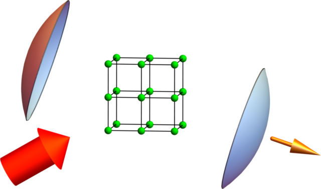
Figure 1: (Color online) Atoms in an optical lattice are probed by a coherent light beam, and the light scattered at a particular angle is enhanced and collected by a leaky cavity. The photons escaping the cavity are detected, perturbing the atomic evolution via measurement backaction.

The isolated system is described by the Bose-Hubbard Model (BHM),

$$\hat{H}_{0}=-J\sum_{\langle i,j\rangle}b^{\dagger}_{i}b_{j}+\frac{U}{2}\sum_{i}\hat{n}_{i}(\hat{n}_{i}-1),$$ (11)

where $b_{i}$ ($b^{\dagger}_{i}$) are the bosonic annihilation (creation) operators at site $i$, $\hat{n}_{i}$ is the atom number operator at site $i$, $U$ is the on-site interaction, and $J$ is the tunnelling coefficient. The optical Hamiltonian is adiabatically eliminated and if the cavity field backaction can be neglected (cavity detuning must be small compared to its decay rate) then its only effect on the system is via measurement backaction Mekhov and Ritsch (2012). The quantum jump operator is given by $\hat{c}=\sqrt{2\kappa}\hat{a}$, where $\kappa$ is the cavity relaxation rate, $\hat{a}=C\hat{D}$ is the annihilation operator of a photon in the cavity mode, $C$ is the coefficient of Rayleigh scattering into the cavity, $\hat{D}=\sum_{i}A_{i}\hat{n}_{i}$, with the coefficients given by $A_{i}=u^{*}_{\mathrm{out}}({\bf r}_{i})u_{\mathrm{in}}({\bf r}_{i})$, and $u_{\mathrm{in,out}}({\bf r}_{i})$ are the mode functions of the incoming and scattered light Mekhov and Ritsch (2012). Additionally, we have the necessary condition to be in the quantum Zeno regime $\gamma/J\gg 1$, where $\gamma=\kappa|C|^{2}$.

We will now consider the simplest case of global multi-site measurement of the form $\hat{D}=\hat{N}_{K}=\sum_{i}^{K}\hat{n}_{i}$, where the sum is over $K$ illuminated sites. Physically, this can be realised by collecting the light scattered into a diffraction maximum Mekhov et al. (2007b, c). The effective Hamiltonian becomes

$$\hat{H}_{\mathrm{eff}}=\hat{H}_{0}-i\gamma\left(\delta\hat{N}_{K}\right)^{2},$$ (12)

where $\delta\hat{N}_{K}=\hat{N}_{K}-N^{0}_{K}$ and $N^{0}_{K}$ is a subspace eigenvalue. It is now obvious that continuous measurement squeezes the fluctuations in the measured quantity, as expected, and that the only competing process is the system’s own dynamics.

In this case, if we adiabatically eliminate the density matrix cross-terms and substitute Eq. (3) into Eq. (II.1) for this system we obtain an effective Hamiltonian within the Zeno subspace defined by $N_{K}$

$$\hat{H}_{\varphi}=P_{\varphi}\left[\hat{H}_{0}-i\frac{J^{2}}{\gamma}\sum_{\begin{subarray}{c}\langle i\in\varphi,j\in\varphi^{\prime}\rangle\\ \langle k\in\varphi^{\prime},l\in\varphi\rangle\end{subarray}}b^{\dagger}_{i}b_{j}b^{\dagger}_{k}b_{l}\right]P_{\varphi},$$ (13)

where $\varphi=\{N_{K}\}$ denotes the set of states with $N_{K}$ atoms in the illuminated area, $\varphi^{\prime}=\{N_{K}\pm 1\}$ denotes the set of intermediate states and $P_{\varphi}$ is the projector onto $\varphi$. We focus on the case when the second term is not only significant, but also leads to dynamics within $\varphi$ that are not allowed by conventional quantum Zeno dynamics accounted for by the first term. The second term represents second-order transitions via other subspaces which act as intermediate states much like virtual states in optical Raman transitions. This is in contrast to the conventional understanding of the Zeno dynamics for infinitely frequent projective measurements (corresponding to $\gamma\rightarrow\infty$) where such processes are forbidden Facchi and Pascazio (2008). Thus, it is the weak quantum measurement that effectively couples the states.

III.2 Small System Example

To get clear physical insight, we initially consider three atoms in three sites and choose our measurement operator such that $\hat{D}=\hat{n}_{2}$, i.e. only the middle site is subject to measurement, and the Zeno subspace defined by $n_{2}=1$. Such an illumination pattern can be achieved with global addressing by crossing two beams and placing the nodes at the odd sites and the antinodes at even sites. This means that $P_{\varphi}\hat{H}_{0}P_{\varphi}=0$. However, the first and third sites are connected via the second term. Diagonalising the Hamiltonian reveals that out of its ten eigenvalues all but three have a significant negative imaginary component of the order $\gamma$ which means that the corresponding eigenstates decay on a time scale of a single quantum jump and thus quickly become negligible. The three remaining eigenvectors are dominated by the linear superpositions of the three Fock states $|2,1,0\rangle$, $|1,1,1\rangle$, and $|0,1,2\rangle$. Whilst it is not surprising that these components are the only ones that remain as they are the only ones that actually lie in the Zeno subspace $n_{2}=1$, it is impossible to solve the full dynamics by just considering these Fock states alone as they are not coupled to each other in $\hat{H}_{0}$. The components lying outside of the Zeno subspace have to be included to allow intermediate steps to occur via states that do not belong in this subspace, much like virtual states in optical Raman transitions.

An approximate solution for $U=0$ can be written for the $\{|2,1,0\rangle,|1,1,1\rangle,|0,1,2\rangle\}$ subspace by multiplying each eigenvector with its corresponding time evolution

$$|\Psi(t)\rangle\propto\left(\begin{array}[]{c}z_{1}+\sqrt{2}z_{2}e^{-6J^{2}t/\gamma}+z_{3}e^{-12J^{2}t/\gamma}\\ -\sqrt{2}\left(z_{1}-z_{3}e^{-12J^{2}t/\gamma}\right)\\ z_{1}-\sqrt{2}z_{2}e^{-6J^{2}t/\gamma}+z_{3}e^{-12J^{2}t/\gamma}\\ \end{array}\right),$$

where $z_{i}$ denote the overlap between the eigenvectors and the initial state, $z_{i}=\langle v_{i}|\Psi(0)\rangle$, with $|v_{1}\rangle=(1,-\sqrt{2},1)/2$, $|v_{2}\rangle=(1,0,-1)/\sqrt{2}$, and $|v_{3}\rangle=(1,\sqrt{2},1)/2$. The steady state as $t\rightarrow\infty$ is given by $|v_{1}\rangle=(1,-\sqrt{2},1)/2$. This solution is illustrated in Fig. 2 which clearly demonstrates dynamics beyond the canonical understanding of quantum Zeno dynamics as tunnelling occurs between states coupled via a different Zeno subspace.

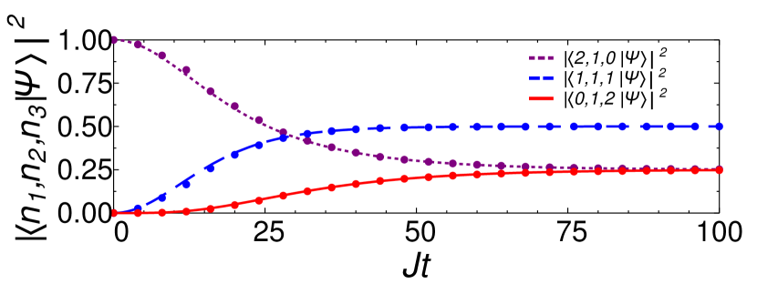
Figure 2: (Color online). Populations of the Fock states in the Zeno subspace for $\gamma/J=100$ and initial state $|2,1,0\rangle$. It is clear that quantum Zeno dynamics occurs via Raman-like processes even though none of these states are connected in $\hat{H}_{0}$. The dynamics occurs via virtual intermediate states outside the Zeno subspace. The system also tends to a steady state which minimises tunnelling effectively suppressing fluctuations. The lines are solutions to the non-Hermitian Hamiltonian, and the dots are points from a stochastic trajectory calculation.

III.3 Steady State of non-Hermitian Dynamics

A distinctive difference between BHM ground states and the final steady state, $[|2,1,0\rangle-\sqrt{2}|1,1,1\rangle+|0,1,2\rangle]$, is that its components are not in phase. Squeezing due to measurement naturally competes with inter-site tunnelling which tends to spread the atoms. However, from Eq. (12) we see the final state will always be the eigenvector with the smallest fluctuations as it will have an eigenvalue with the largest imaginary component. This naturally corresponds to the state where tunnelling between Zeno subspaces (here between every site) is minimised by destructive matter-wave interference, i.e. the tunnelling dark state defined by $\hat{T}|\Psi\rangle=0$, where $\hat{T}=\sum_{\langle i,j\rangle}b^{\dagger}_{i}b_{j}$. This is simply the physical interpretation of the steady states we predicted for Eq. (II.1). Crucially, this state can only be reached if the dynamics aren’t fully suppressed by measurement and thus, counter-intuitively, the atomic dynamics cooperate with measurement to suppress itself by destructive interference. Therefore, this effect is beyond the scope of traditional quantum Zeno dynamics and presents a new perspective on the competition between a system’s short-range dynamics and global measurement backaction.

We now consider a one-dimensional lattice with $M$ sites so we extend the measurement to $\hat{D}=\hat{N}_{\text{even}}$ where every even site is illuminated (obtained by crossing two beams such that the nodes coincide with odd sites and antinodes with even sites Mekhov et al. (2007c); Mazzucchi et al. (2016a)). The wavefunction in a Zeno subspace must be an eigenstate of $\hat{c}$ and we combine this with the requirement for it to be in the dark state of the tunnelling operator (eigenstate of $\hat{H}_{0}$ for $U=0$) to derive the steady state. These two conditions in momentum space are

$$\hat{T}|\Psi\rangle=\sum_{\text{RBZ}}\left[b^{\dagger}_{k}b_{k}-b^{\dagger}_{q}b_{q}\right]\cos(ka)|\Psi\rangle=0,$$

$$\Delta\hat{N}|\Psi\rangle=\sum_{\text{RBZ}}\left[b^{\dagger}_{k}b_{-q}+b^{\dagger}_{-q}b_{k}\right]|\Psi\rangle=\Delta N|\Psi\rangle,$$

where $b_{k}=\frac{1}{\sqrt{M}}\sum_{j}e^{ikja}b_{j}$, $\Delta\hat{N}=\hat{D}-N/2$, $q=\pi/a-k$, $a$ is the lattice spacing, $N$ the total atom number, and we perform summations over the reduced Brillouin zone (RBZ), $-\pi/2a<k\leq\pi/2a$, as the symmetries of the system are clearer this way. Now we define

$$\hat{\alpha}_{k}^{\dagger}=b^{\dagger}_{k}b^{\dagger}_{q}-b^{\dagger}_{-k}b^{\dagger}_{-q},$$ (14)

$$\hat{\beta}_{\varphi}^{\dagger}=b^{\dagger}_{\pi/2a}+\varphi b^{\dagger}_{-\pi/2a},$$ (15)

where $\varphi=\Delta N/|\Delta N|$, which create the smallest possible states that satisfy the two equations for $\Delta N=0$ and $\Delta N\neq 0$ respectively. Therefore, by noting that $\left[\hat{T},\hat{\alpha}_{k}^{\dagger}\right]=\left[\Delta\hat{N},\hat{\alpha}_{k}^{\dagger}\right]=\left[\hat{T},\hat{\beta}_{\varphi}^{\dagger}\right]=0$ and $\left[\Delta\hat{N},\hat{\beta}_{\varphi}^{\dagger}\right]=\varphi\hat{\beta}_{\varphi}^{\dagger}$ we can now write the equation for the $N$-particle steady state

$$|\Psi\rangle\propto\left[\prod_{i=1}^{(N-|\Delta N|)/2}\left(\sum_{k=0}^{\pi/2a}\phi_{i,k}\hat{\alpha}_{k}^{\dagger}\right)\right]\left(\hat{\beta}_{\varphi}^{\dagger}\right)^{|\Delta N|}|0\rangle,$$

where $\phi_{i,k}$ are coefficients that depend on the trajectory taken to reach this state and $|0\rangle$ is the vacuum state defined by $b_{k}|0\rangle=0$. Since this a dark state (an eigenstate of $\hat{H}_{0}$) of the atomic dynamics, this state will remain stationary even with measurement switched-off. Interestingly, this state is very different from the ground states of the BHM, it is even orthogonal to the superfluid state, and thus it cannot be obtained by cooling or projecting from an initial ground state. The combination of tunnelling with measurement is necessary.

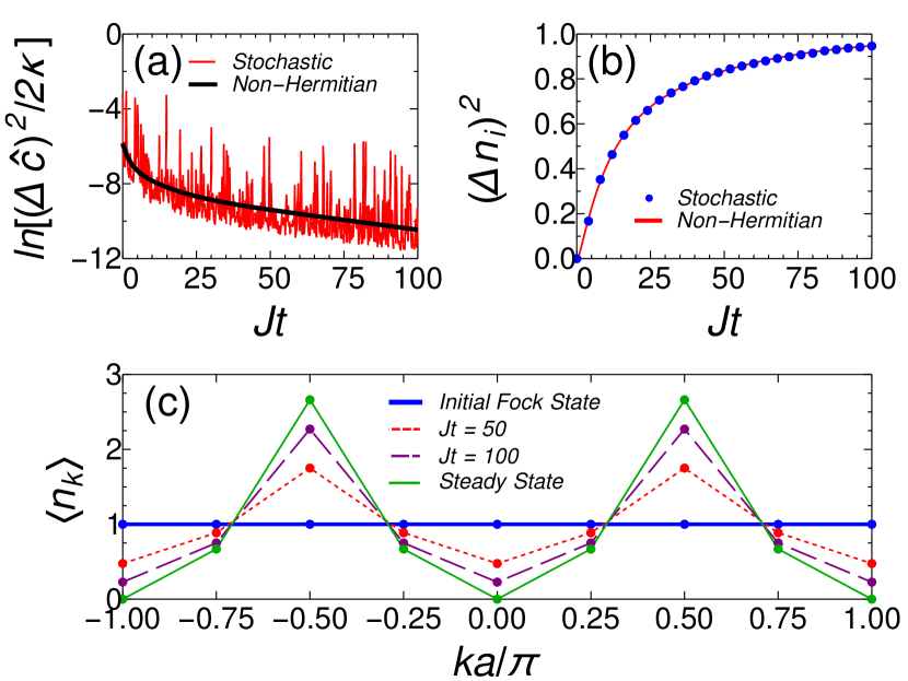
Figure 3: (Color online). A trajectory simulation for eight atoms in eight sites, initially in $|1,1,1,1,1,1,1,1\rangle$, with periodic boundary conditions and $\gamma/J=100$. (a), The fluctuations in $\hat{c}$ where the stochastic nature of the process is clearly visible on a single trajectory level. However, the general trend is captured by the non-Hermitian Hamiltonian. (b), The local density variance. Whilst the fluctuations in the global measurement operator decrease, the fluctuations in local density increase due to tunnelling via states outside the Zeno subspace. (c), The momentum distribution. The initial Fock state has a flat distribution which with time approaches the steady state distribution of two identical and symmetric distributions centred at $k=\pi/2a$ and $k=-\pi/2a$.

In order to prepare the steady state one has to run the experiment and wait until the photocount rate remains constant for a sufficiently long time. Such a trajectory is illustrated in Fig. 3 and compared to a deterministic trajectory calculated using the non-Hermitian Hamiltonian. It is easy to see from Fig. 3(a) how the stochastic fluctuations around the mean value of the observable have no effect on the general behaviour of the system in the strong measurement regime. By discarding these fluctuations we no longer describe a pure state, but we showed how this only leads to a negligible error. Fig. 3(b) shows the local density variance in the lattice. Not only does it grow showing evidence of tunnelling between illuminated and non-illuminated sites, but it grows to significant values. This is in contrast to conventional quantum Zeno dynamics where no tunnelling would be allowed at all. Finally, Fig. 3(c) shows the momentum distribution of the trajectory. We can clearly see that it deviates significantly from the initial flat distribution of the Fock state. Furthermore, the steady state does not have any atoms in the $k=0$ state and thus is orthogonal to the superfluid state as discussed.

To obtain a state with a specific value of $\Delta N$ postselection may be necessary, but otherwise it is not needed. The process can be optimised by feedback control since the state is monitored at all times Ivanov and Ivanova (2014). Furthermore, the form of the measurement operator is very flexible and it can easily be engineered by the geometry of the optical setup Elliott et al. (2015a); Mazzucchi et al. (2016a) which can be used to design a state with desired properties.

IV Summary

In summary, we have presented a new perspective on quantum Zeno dynamics when the measurement isn’t fully projective. By using the fact that the system is strongly confined to a specific measurement eigenspace we have derived an effective non-Hermitian Hamiltonian. In contrast to previous works, it is independent of the underlying system and there is no need to postselect for a particular exotic trajectory Lee and Chan (2014); Lee et al. (2014). Using the BHM as an example we have shown that whilst the system remains in its Zeno subspace, it will exhibit Raman-like transitions within this subspace which would be forbidden in the canonical fully projective limit. Finally, we have shown that the system will always tend towards the eigenstate of the Hamiltonian with the best squeezing in the measured quantity and the atomic dynamics, which normally tend to spread the distribution, cooperates with measurement to produce a state in which tunnelling is suppressed by destructive matter-wave interference. A dark state of the tunnelling operator will have zero fluctuations and we provided an expression for the steady state which is significantly different from the ground state of the Hamiltonian. This is in contrast to previous works on dissipative state preparation where the steady state had to be a dark state of the measurement operator instead Diehl et al. (2008).

Appendix A Determining the Zeno subspace

Following the main text we now consider how to estimate the Zeno subspace. Since the density matrix cross-terms are small we know a priori that the individual wavefunctions comprising the density matrix mixture will not be coherent superpositions of different Zeno subspaces. Therefore, each individual experiment will at any time be predominantly in a single Zeno subspace with small cross-terms and negligible occupations in the other subspaces. With no measurement record our density matrix would be a mixture of all these possibilities. However, we can try and determine the Zeno subspace around which the state evolves in a single experiment from the number of detections, $m$, in time $t$.

The detection distribution on time-scales shorter than dissipation (so we can approximate as if we were in a fully Zeno regime) can be obtained by integrating over the detection times Mekhov and Ritsch (2009c) to get

$$P(m,t)=\sum_{n}\frac{[|c_{n}|^{2}t]^{m}}{m!}e^{-|c_{n}|^{2}t}\mathrm{Tr}(\rho_{nn}).$$ (16)

For a state that is predominantly in one Zeno subspace, the distribution will be approximately Poissonian (up to $\mathcal{O}(K^{2}/\lambda^{4}$), the population of the other subspaces). Therefore, in a single experiment we will measure $m=|c_{0}|^{2}t\pm\sqrt{|c_{0}|^{2}t}$ detections (note, we have assumed $|c_{0}|^{2}t$ is large enough to approximate the distribution as normal. This is not necessary, we simply use it here to not have to worry about the asymmetry in the deviation around the mean value). The uncertainty does not come from the fact that $\lambda$ is not infinite. The jumps are random events with a Poisson distribution. Therefore, even in the full projective limit we will not observe the same detection trajectory in each experiment even though the system evolves in exactly the same way and remains in a perfectly pure state.

If the basis of $\hat{c}$ is continuous (e.g. free particle position or momentum) then the deviation around the mean will be our upper bound on the deviation of the system from a pure state evolving around a single Zeno subspace. However, continuous systems are beyond the scope of this work and we will confine ourselves to discrete systems. Though it is important to remember that continuous systems can be treated this way, but the error estimate (and thus the mixedness of the state) will be different.

For a discrete system it is easier to exclude all possibilities except for one. The error in our estimate of $|c_{0}|^{2}$ in a single experiment decreases as $1/\sqrt{t}$ and thus it can take a long time to confidently determine $|c_{0}|^{2}$ to a sufficient precision this way. However, since we know that it can only take one of the possible values from the set $\{|c_{n}|^{2}\}$ it is much easier to exclude all the other values.

In an experiment we can use Bayes’ theorem to infer the state of our system as follows

$$p(c_{n}=c_{0}|m)=\frac{p(m|c_{n}=c_{0})p(c_{n}=c_{0})}{p(m)},$$ (17)

where $p(x)$ denotes the probability of the discrete event $x$ and $p(x|y)$ the conditional probability of $x$ given $y$. We know that $p(m|c_{n}=c_{0})$ is simply given by a Poisson distribution with mean $|c_{0}|^{2}t$. $p(m)$ is just a normalising factor and $p(c_{n}=c_{0})$ is our a priori knowledge of the state. Therefore, one can get the probability of being in the right Zeno subspace from

$$p(c_{n} =c_{0}|m)=\frac{p_{0}(c_{n}=c_{0})\frac{\left(|c_{0}|^{2}t\right)^{2m}}{m!}e^{-|c_{0}|^{2}t}}{\sum_{n}p_{0}(c_{n})\frac{\left(|c_{n}|^{2}t\right)^{2m}}{m!}e^{-|c_{n}|^{2}t}}$$

$$=p_{0}(c_{n}=c_{0})\left[\sum_{n}p_{0}(c_{n})\left(\frac{|c_{n}|^{2}}{|c_{0}|^{2}}\right)^{2m}e^{\left(|c_{0}|^{2}-|c_{n}|^{2}\right)t}\right]^{-1},$$ (18)

where $p_{0}$ denotes probabilities at $t=0$. In a real experiment one could prepare the initial state to be close to the Zeno subspace of interest and thus it would be easier to deduce the state. Furthermore, in the middle of an experiment if we have already established the Zeno subspace this will be reflected in these a priori probabilities again making it easier to infer the correct subspace. However, we will consider the worst case scenario which might be useful if we don’t know the initial state or if the Zeno subspace changes during the experiment, a uniform $p_{0}(c_{n})$.

This probability is a rather complicated function as $m$ is a stochastic quantity that also increases with $t$. We want it to be as close to 1 as possible. In order to devise an appropriate condition for this we note that in the first line all terms in the denominator are Poisson distributions of $m$. Therefore, if the mean values $|c_{n}|^{2}t$ are sufficiently spaced out, only one of the terms in the sum will be significant for a given $m$ and if this happens to be the one that corresponds to $c_{0}$ we get a probability close to unity. Therefore, we set the condition such that it is highly unlikely that our measured $m$ could be produced by two different distributions

$$\sqrt{|c_{0}|^{2}t}\ll||c_{0}|^{2}-|c_{n}|^{2}||t,\forall n\neq 0$$ (19)

$$\sqrt{|c_{n}|^{2}t}\ll||c_{0}|^{2}-|c_{n}|^{2}||t,\forall n\neq 0$$ (20)

The LHS is the standard deviation of $m$ if the system was in subspace $P_{0}$ or $P_{n}$. The RHS is the difference in the mean detections between the subspace $n$ and the one we are interested in. The condition becomes more strict if the subspaces become less distinguishable as it becomes harder to confidently determine the correct state. Once again, using $\hat{c}=\lambda\hat{o}$ where $\hat{o}\sim\mathcal{O}(1)$ we get

$$t\gg\frac{1}{\lambda^{2}}\frac{|o_{0,n}|^{2}}{(|o_{0}|^{2}-|o_{n}|^{2}|)^{2}}.$$ (21)

Since detections happen on average at an average rate of order $\lambda^{2}$ we only need to wait for a few detections to satisfy this condition. Therefore, we see that even in the worst case scenario of complete ignorance of the state of the system we can very easily determine the correct subspace. Once it is established for the first time, the a priori information can be updated and it will become even easier to monitor the system.

However, it is important to note that physically once the quantum jumps deviate too much from the mean value the system is more likely to change the Zeno subspace (due to measurement backaction) and the detection rate will visibly change. Therefore, if we observe a consistent detection rate it is extremely unlikely that it can be produced by two different Zeno subspaces so in fact it is even easier to determine the correct state, but the above estimate serves as a good lower bound on the necessary detection time.

References

- Misra and Sudarshan (1977) B. Misra and E. C. G. Sudarshan, J. Math. Phys. 18, 756 (1977).
- Facchi and Pascazio (2008) P. Facchi and S. Pascazio, J. Phys. A: Math. Theor. 41, 493001 (2008).
- Itano et al. (1990) W. M. Itano, D. J. Heinzen, J. J. Bollinger, and D. J. Wineland, Phys. Rev. A 41, 2295 (1990).
- Nagels et al. (1997) B. Nagels, L. J. F. Hermans, and P. L. Chapovsky, Phys. Rev. Lett. 79, 3097 (1997).
- Kwiat et al. (1999) P. G. Kwiat, A. G. White, J. R. Mitchell, O. Nairz, G. Weihs, H. Weinfurter, and A. Zeilinger, Phys. Rev. Lett. 83, 4725 (1999).
- Balzer et al. (2000) C. Balzer, R. Huesmann, W. Neuhauser, and P. Toschek, Optics Communications 180, 115 (2000).
- Streed et al. (2006) E. W. Streed, J. Mun, M. Boyd, G. K. Campbell, P. Medley, W. Ketterle, and D. E. Pritchard, Phys. Rev. Lett. 97, 260402 (2006).
- Hosten et al. (2006) O. Hosten, M. T. Rakher, J. T. Barreiro, N. A. Peters, and P. G. Kwiat, Nature 439, 949 (2006).
- Bernu et al. (2008) J. Bernu, S. Deléglise, C. Sayrin, S. Kuhr, I. Dotsenko, M. Brune, J. M. Raimond, and S. Haroche, Phys. Rev. Lett. 101, 180402 (2008).
- Raimond et al. (2010) J. M. Raimond, C. Sayrin, S. Gleyzes, I. Dotsenko, M. Brune, S. Haroche, P. Facchi, and S. Pascazio, Phys. Rev. Lett. 105, 213601 (2010).
- Raimond et al. (2012) J. M. Raimond, P. Facchi, B. Peaudecerf, S. Pascazio, C. Sayrin, I. Dotsenko, S. Gleyzes, M. Brune, and S. Haroche, Phys. Rev. A 86, 032120 (2012).
- Signoles et al. (2014) A. Signoles, A. Facon, D. Grosso, I. Dotsenko, S. Haroche, J.-M. Raimond, M. Brune, and S. Gleyzes, Nat. Phys. 10, 715 (2014).
- Hatano and Nelson (1996) N. Hatano and D. R. Nelson, Phys. Rev. Lett. 77, 570 (1996).
- Refael et al. (2006) G. Refael, W. Hofstetter, and D. R. Nelson, Phys. Rev. B 74, 174520 (2006).
- Bender and Boettcher (1998) C. M. Bender and S. Boettcher, Phys. Rev. Lett. 80, 5243 (1998).
- Giorgi (2010) G. L. Giorgi, Phys. Rev. B 82, 052404 (2010).
- Zhang and Song (2013) X. Z. Zhang and Z. Song, Phys. Rev. A 87, 012114 (2013).
- Otterbach and Lemeshko (2014) J. Otterbach and M. Lemeshko, Phys. Rev. Lett. 113, 070401 (2014).
- Lee and Chan (2014) T. E. Lee and C.-K. Chan, Phys. Rev. X 4, 041001 (2014).
- Lee et al. (2014) T. E. Lee, F. Reiter, and N. Moiseyev, Phys. Rev. Lett. 113, 250401 (2014).
- Dembowski et al. (2001) C. Dembowski, H.-D. Gräf, H. L. Harney, A. Heine, W. D. Heiss, H. Rehfeld, and A. Richter, Phys. Rev. Lett. 86, 787 (2001).
- Choi et al. (2010) Y. Choi, S. Kang, S. Lim, W. Kim, J.-R. Kim, J.-H. Lee, and K. An, Phys. Rev. Lett. 104, 153601 (2010).
- Ruter et al. (2010) C. E. Ruter, K. G. Makris, R. El-Ganainy, D. N. Christodoulides, M. Segev, and D. Kip, Nat. Phys. 6, 192 (2010).
- Barontini et al. (2013) G. Barontini, R. Labouvie, F. Stubenrauch, A. Vogler, V. Guarrera, and H. Ott, Phys. Rev. Lett. 110, 035302 (2013).
- Gao et al. (2015) T. Gao, E. Estrecho, K. Bliokh, T. Liew, M. Fraser, S. Brodbeck, M. Kamp, C. Schneider, S. Höfling, Y. Yamamoto, et al., Nature advance online publication (2015).
- Dhar et al. (2015) S. Dhar, S. Dasgupta, A. Dhar, and D. Sen, Phys. Rev. A 91, 062115 (2015).
- Stannigel et al. (2014) K. Stannigel, P. Hauke, D. Marcos, M. Hafezi, S. Diehl, M. Dalmonte, and P. Zoller, Physical review letters 112, 120406 (2014).
- Bloch et al. (2007) I. Bloch, J. Dalibard, and W. Zwerger, Rev. Mod. Phys. 80, 885 (2007).
- Lewenstein et al. (2007) M. Lewenstein, A. Sanpera, V. Ahufinger, B. Damski, A. Sen(De), and U. Sen, Advances in Physics 56, 243 (2007).
- Ritsch et al. (2013) H. Ritsch, P. Domokos, F. Brennecke, and T. Esslinger, Rev. Mod. Phys. 85, 553 (2013).
- Mekhov and Ritsch (2012) I. B. Mekhov and H. Ritsch, J. Phys. B At. Mol. Opt. Phys. 45, 102001 (2012).
- Ruostekoski and Walls (1997) J. Ruostekoski and D. F. Walls, Physical Review A 56, 2996 (1997).
- Mekhov et al. (2007a) I. B. Mekhov, C. Maschler, and H. Ritsch, Nat. Phys. 3, 319 (2007a).
- Chen and Meystre (2009) W. Chen and P. Meystre, Phys. Rev. A 79, 043801 (2009).
- Mekhov and Ritsch (2009a) I. B. Mekhov and H. Ritsch, Laser physics 19, 610 (2009a).
- Mekhov and Ritsch (2010) I. B. Mekhov and H. Ritsch, Laser physics 20, 694 (2010).
- Mekhov and Ritsch (2011) I. B. Mekhov and H. Ritsch, Laser Physics 21, 1486 (2011).
- Mekhov (2013) I. B. Mekhov, Laser Physics 23, 015501 (2013).
- Pedersen et al. (2014) M. K. Pedersen, J. J. W. Sørensen, M. C. Tichy, and J. F. Sherson, New Journal of Physics 16, 113038 (2014).
- Elliott et al. (2015a) T. J. Elliott, W. Kozlowski, S. F. Caballero-Benitez, and I. B. Mekhov, Phys. Rev. Lett. 114, 113604 (2015a).
- Kozlowski et al. (2015) W. Kozlowski, S. F. Caballero-Benitez, and I. B. Mekhov, Phys. Rev. A 92, 013613 (2015).
- Mazzucchi et al. (2016a) G. Mazzucchi, W. Kozlowski, S. F. Caballero-Benitez, T. J. Elliott, and I. B. Mekhov, Phys. Rev. A 93, 023632 (2016a).
- Elliott et al. (2015b) T. J. Elliott, G. Mazzucchi, W. Kozlowski, S. F. Caballero-Benitez, and I. B. Mekhov, Atoms 3, 392 (2015b).
- Wade et al. (2015) A. C. J. Wade, J. F. Sherson, and K. Mølmer, Phys. Rev. Lett. 115, 060401 (2015).
- Ashida and Ueda (2015) Y. Ashida and M. Ueda, Phys. Rev. Lett. 115, 095301 (2015).
- Mazzucchi et al. (2016b) G. Mazzucchi, W. Kozlowski, S. F. Caballero-Benitez, and I. B. Mekhov, New Journal of Physics 18, 073017 (2016b).
- Caballero-Benitez et al. (2016) S. F. Caballero-Benitez, G. Mazzucchi, and I. B. Mekhov, Phys. Rev. A 93, 063632 (2016).
- Baumann et al. (2010) K. Baumann, C. Guerlin, F. Brennecke, and T. Esslinger, Nature 464, 1301 (2010).
- Wolke et al. (2012) M. Wolke, J. Klinner, H. Keßler, and A. Hemmerich, Science 337, 75 (2012).
- Schmidt et al. (2014) D. Schmidt, H. Tomczyk, S. Slama, and C. Zimmermann, Phys. Rev. Lett. 112, 115302 (2014).
- Miyake et al. (2011) H. Miyake, G. A. Siviloglou, G. Puentes, D. E. Pritchard, W. Ketterle, and D. M. Weld, Phys. Rev. Lett. 107, 175302 (2011).
- Weitenberg et al. (2011) C. Weitenberg, M. Endres, J. F. Sherson, M. Cheneau, P. Schauss, T. Fukuhara, I. Bloch, and S. Kuhr, Nature 471, 319 (2011).
- Landig et al. (2016) R. Landig, L. Hruby, N. Dogra, M. Landini, R. Mottl, T. Donner, and T. Esslinger, Nature (2016).
- Klinder et al. (2015) J. Klinder, H. Keßler, M. R. Bakhtiari, M. Thorwart, and A. Hemmerich, Physical Review Letters 115, 230403 (2015).
- Mekhov et al. (2007b) I. B. Mekhov, C. Maschler, and H. Ritsch, Phys. Rev. Lett. 98, 100402 (2007b).
- Mekhov et al. (2007c) I. B. Mekhov, C. Maschler, and H. Ritsch, Phys. Rev. A 76, 053618 (2007c).
- Eckert et al. (2008) K. Eckert, O. Romero-Isart, M. Rodriguez, M. Lewenstein, E. S. Polzik, and A. Sanpera, Nat. Phys. 4, 50 (2008).
- Roscilde et al. (2009) T. Roscilde, M. Rodríguez, K. Eckert, O. Romero-Isart, M. Lewenstein, E. Polzik, and A. Sanpera, New Jour. Phys. 11, 055041 (2009).
- Mekhov and Ritsch (2009b) I. B. Mekhov and H. Ritsch, Phys. Rev. Lett. 102, 020403 (2009b).
- Mekhov and Ritsch (2009c) I. B. Mekhov and H. Ritsch, Phys. Rev. A 80, 013604 (2009c).
- De Chiara et al. (2011) G. De Chiara, O. Romero-Isart, and A. Sanpera, Phys. Rev. A 83, 021604 (2011).
- Hauke et al. (2013) P. Hauke, R. J. Sewell, M. W. Mitchell, and M. Lewenstein, Phys. Rev. A 87, 021601 (2013).
- Rogers et al. (2014) B. Rogers, M. Paternostro, J. F. Sherson, and G. De Chiara, Phys. Rev. A 90, 043618 (2014).
- Nagy et al. (2008) D. Nagy, G. Szirmai, and P. Domokos, The European Physical Journal D 48, 127 (2008).
- Niedenzu et al. (2013) W. Niedenzu, S. Schütz, H. Habibian, G. Morigi, and H. Ritsch, Physical Review A 88, 033830 (2013).
- Bakhtiari et al. (2015) M. R. Bakhtiari, A. Hemmerich, H. Ritsch, and M. Thorwart, Phys. Rev. Lett. 114, 123601 (2015).
- Ivanov and Ivanova (2015) D. Ivanov and T. Y. Ivanova, J. Exp. Theor. Phys. 121, 179 (2015).
- Schütz et al. (2015) S. Schütz, S. B. Jäger, and G. Morigi, arXiv:1508.06606 (2015).
- Winterauer et al. (2015) D. J. Winterauer, W. Niedenzu, and H. Ritsch, Physical Review A 91, 053829 (2015).
- Piazza and Ritsch (2015) F. Piazza and H. Ritsch, Phys. Rev. Lett. 115, 163601 (2015).
- Wiseman and Milburn (2010) H. M. Wiseman and G. J. Milburn, Quantum Measurement and Control (Cambridge University Press, 2010).
- Diehl et al. (2008) S. Diehl, A. Micheli, A. Kantian, B. Kraus, H. Büchler, and P. Zoller, Nat. Phys. 4, 878 (2008).
- Bux et al. (2013) S. Bux, H. Tomczyk, D. Schmidt, P. W. Courteille, N. Piovella, and C. Zimmermann, Phys. Rev. A 87, 023607 (2013).
- Keßler et al. (2014) H. Keßler, J. Klinder, M. Wolke, and A. Hemmerich, Phys. Rev. Lett. 113, 070404 (2014).
- Landig et al. (2015) R. Landig, F. Brennecke, R. Mottl, T. Donner, and T. Esslinger, Nat. Comms. 6 (2015).
- Caballero-Benitez and Mekhov (2015a) S. F. Caballero-Benitez and I. B. Mekhov, Phys. Rev. Lett. 115, 243604 (2015a).
- Caballero-Benitez and Mekhov (2015b) S. F. Caballero-Benitez and I. B. Mekhov, New Journal of Physics 17, 123023 (2015b).
- Pichler et al. (2010) H. Pichler, A. J. Daley, and P. Zoller, Phys. Rev. A 82, 063605 (2010).
- Sarkar et al. (2014) S. Sarkar, S. Langer, J. Schachenmayer, and A. J. Daley, Phys. Rev. A 90, 023618 (2014).
- Syassen et al. (2008) N. Syassen, D. M. Bauer, M. Lettner, T. Volz, D. Dietze, J. J. Garcia-Ripoll, J. I. Cirac, G. Rempe, and S. Dürr, Science 320, 1329 (2008).
- Kepesidis and Hartmann (2012) K. V. Kepesidis and M. J. Hartmann, Phys. Rev. A 85, 063620 (2012).
- Vidanović et al. (2014) I. Vidanović, D. Cocks, and W. Hofstetter, Phys. Rev. A 89, 053614 (2014).
- Bernier et al. (2014) J.-S. Bernier, D. Poletti, and C. Kollath, Phys. Rev. B 90, 205125 (2014).
- Daley (2014) A. J. Daley, Adv. Phys. 63, 77 (2014).
- Ates et al. (2012) C. Ates, B. Olmos, W. Li, and I. Lesanovsky, Phys. Rev. Lett. 109, 233003 (2012).
- Everest et al. (2014) B. Everest, M. R. Hush, and I. Lesanovsky, Phys. Rev. B 90, 134306 (2014).
- Bretheau et al. (2015) L. Bretheau, P. Campagne-Ibarcq, E. Flurin, F. Mallet, and B. Huard, Science 348, 776 (2015).
- Ivanov and Ivanova (2014) D. Ivanov and T. Y. Ivanova, JETP letters 100, 481 (2014).