A Semantic Theory of the Internet of Things

Abstract

We propose a process calculus for modelling systems in the Internet of Things paradigm. Our systems interact both with the physical environment, via sensors and actuators, and with smart devices, via short-range and Internet channels. The calculus is equipped with a standard notion of bisimilarity which is a fully abstract characterisation of a well-known contextual equivalence. We use our semantic proof-methods to prove run-time properties as well as system equalities of non-trivial IoT systems.

1 Introduction

In the Internet of Things (IoT) paradigm, smart devices, such as smartphones, automatically collect information from shared resources (e.g. Internet access or physical devices) and aggregate them to provide new services to end users [16]. The “things” commonly deployed in IoT systems are: RFID tags, for unique identification, sensors, to detect physical changes in the environment, and actuators, to pass information to the environment.

The research on IoT is currently focusing on practical applications such as the development of enabling technologies [32], ad hoc architectures [30], semantic web technologies [9], and cloud computing [16]. However, as pointed out by Lanese et al. [20], there is a lack of research in formal methodologies to model the interactions among system components, and to verify the correctness of the network deployment before its implementation. Lanese et al. proposed the first process calculus for IoT systems, called IoT-calculus [20]. The IoT-calculus captures the partial topology of communications and the interaction between sensors, actuators and computing processes to provide useful services to the end user. A behavioural equivalence is then defined to compare IoT systems.

Devising a calculus for modelling a new paradigm requires understanding and distilling in a clean algebraic setting the main features of the paradigm. The main goal of this paper is to propose a new process calculus that integrates a number of crucial features not addressed in the IoT-calculus, and equipped with a clearly-defined semantic theory for specifying and reasoning on IoT applications. Let us try to figure out what are the main ingredients of IoT, by means of an example.

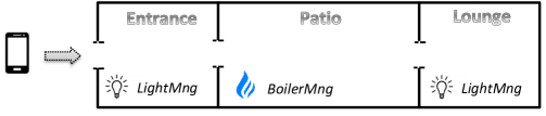
Figure 1: A simple smart home

Suppose a simple smart home in which the user can use her smartphone to remotely control the heating boiler of her house, and automatically turn on lights when entering a room. In Fig. 1, we draw a small smart home with an entrance and a lounge, separated by a patio. Entrance and lounge have their own lights (actuators) which are governed by different light manager processes, $LightMng$. The boiler is in the patio and is governed by a boiler manager process, $BoilerMng$. This process senses the local temperature (via a sensor) and decides whether the boiler should be turned on/off, by setting a proper actuator to signal the state of the boiler.

The smartphone executes two processes: $BoilerCtrl$ and $LightCtr$. The first one reads user’s commands, submitted via the phone touchscreen (a sensor), and forward them to the process $BoilerMng$, via an Internet channel. Whereas, the process $LightCtrl$ interacts with the processes $LightMng$, via short-range wireless channels (e.g. Bluetooth), to automatically turn on lights when the smartphone physically enters either the entrance or the lounge.

The whole system is given by the parallel composition of the smartphone (a mobile device) and the smart home (a stationary entity).

Now, on such kind of systems one may wish to prove run-time properties. Think of a fairness property saying that the boiler will be eventually turned on/off whenever some conditions are satisfied. Or consistency properties, saying the smartphone will never be in two rooms at the same time. Even more, one may be interested in understanding whether our system has the same observable behaviour of another system. Think of a variant of our smart home, where lights functionality depends on GPS coordinates of the smartphone (localisation is a common feature of today smartphones). Intuitively, the smartphone might send its GPS position to a centralised light manager, ${CL}ightMng$ (possibly placed in the patio), via an Internet channel. The process ${CL}ightMng$ will then interact with the two processes $LightMng$, via short-range channels, to switch on/off lights, depending on the position of the smartphone. Here comes an interesting question: Can these two implementations, based on different light management mechanisms, be actually distinguished by an end user?

In the paper at hand we develop a fully abstract semantic theory for a process calculus of IoT systems, called CaIT. We provide a formal notion of when two systems in CaIT  are indistinguishable, in all possible contexts, from the point of view of the end user. Formally, we use the approach of [18, 33], often called reduction (closed) barbed congruence, which relies on two crucial concepts: a reduction semantics, to describe system computations, and the basic observables, to represent what the environment can directly observe of a system. In CaIT, there here are at least two possible observables: the ability to transmit along channels, logical observation, and the capability to diffuse messages via actuators, physical observation. We have adopted the second form as our contextual equality remains invariant when adding logical observation. However, the right definition of physical observation is far from obvious as it involves some technical challenges in the definition of the reduction semantics (see the discussion in Sec. 2.3).

Our calculus is equipped with two labelled transition semantics (LTS) in the SOS style of Plotkin [31]: an intensional semantics and an extensional semantics. The adjective intensional is used to stress the fact that the actions here correspond to activities which can be performed by a system in isolation, without any interaction with the external environment. While, the extensional semantics focuses on those activities which require a contribution of the environment. Our extensional LTS builds on the intensional one, byintroducing specific transitions for modelling all interactions which a system can have with its environment. Here, we would like to point out that since our basic observation on systems does not involve the recording of the passage of time, this has to be taken into account extensionally in order to gain a proper extensional account of systems.

As a first result we prove that the reduction semantics coincides with the intensional semantics (Harmony Theorem), and that they satisfy some desirable time properties such as time determinism, patience, maximal progress and well-timedness [17].

However, the main result of the paper is that weak bisimilarity in the extensional LTS is sound and complete with respect to our contextual equivalence, reduction barbed congruence: two systems are related by some bisimulation in the extensional LTS if and only if they are contextually equivalent. This required a non-standard proof of the congruence theorem (Thm. 3). Finally, in order to show the effectiveness of our bisimulation proof method, we prove a number of non-trivial system equalities.

Outline

Sec. 2 contains the calculus together with the reduction semantics, the contextual equivalence, and a discussion on design choices. Sec. 3 gives the details of our smart home example, and provides desirable run-time properties for it. Sec. 4 defines both intensional and extensional LTSs. In Sec. 5 we define bisimilarity for IoT-systems, and prove the full abstraction result together with a number of non-trivial system equalities. Sec. 6 discusses related work, and concludes.

2 The calculus

In Tab. 1 we give the syntax of our Calculus for the Internet of Things, shortly CaIT, in a two-level structure: a lower one for processes and an upper one for networks of smart devices. We use letters $n,m$ to denote nodes/devices, $c,g$ for channels, $h,k$ for (physical) locations, $s,s^{\prime}$ for sensors, $a,a^{\prime}$ for actuators and $x,y,z$ for variables. Our values, ranged over by $v$ and $w$, are constituted by basic values, such as booleans and integers, sensor and actuator values, and coordinates of physical locations.

$\begin{array}[]{@{\hspace*{2mm}}rcl@{\hspace*{10mm}}l@{\hspace*{4mm}}rcl@{\hspace*{2mm}}l}\lx@intercol\textit{Network:}\hfil\lx@intercol\\ \hskip 5.69054pt\lx@intercol\hfil M,N&\>\;::=&\boldsymbol{0}\hfil\hskip 28.45274pt&\mbox{empty network}\hfil\hskip 11.38109pt\\ \hskip 5.69054pt\lx@intercol\hfil&\quad\big{|}&n{\boldsymbol{[}\mathcal{I}{\Join}P\boldsymbol{]}}^{\mu}_{h}\hfil\hskip 28.45274pt&\mbox{node/device}\hfil\hskip 11.38109pt\\ \hskip 5.69054pt\lx@intercol\hfil&\quad\big{|}&M|N\hfil\hskip 28.45274pt&\mbox{network composition}\hfil\hskip 11.38109pt\\ \hskip 5.69054pt\lx@intercol\hfil&\quad\big{|}&({\boldsymbol{\nu}}c)M\hfil\hskip 28.45274pt&\mbox{channel restriction}\hfil\hskip 11.38109pt\\[1.0pt] \lx@intercol\textit{Process:}\hfil\lx@intercol\\ \hskip 5.69054pt\lx@intercol\hfil P,Q&\>\;::=&\mathsf{nil}\hfil\hskip 28.45274pt&\mbox{termination}\hfil\hskip 11.38109pt\\ \hskip 5.69054pt\lx@intercol\hfil&\quad\big{|}&\rho.P\hfil\hskip 28.45274pt&\mbox{prefixing}\hfil\hskip 11.38109pt\\ \hskip 5.69054pt\lx@intercol\hfil&\quad\big{|}&P|Q\hfil\hskip 28.45274pt&\mbox{parallel composition}\hfil\hskip 11.38109pt\\ \hskip 5.69054pt\lx@intercol\hfil&\quad\big{|}&\lfloor\pi.P\rfloor Q\hfil\hskip 28.45274pt&\mbox{communication with timeout}\hfil\hskip 11.38109pt\\ \hskip 5.69054pt\lx@intercol\hfil&\quad\big{|}&[b]P;Q\hfil\hskip 28.45274pt&\mbox{conditional}\hfil\hskip 11.38109pt\\ \hskip 5.69054pt\lx@intercol\hfil&\quad\big{|}&X\hfil\hskip 28.45274pt&\mbox{process variable}\hfil\hskip 11.38109pt\\ \hskip 5.69054pt\lx@intercol\hfil&\quad\big{|}&{\mathsf{fix}}\,X.P\hfil\hskip 28.45274pt&\mbox{recursion}\hfil\hskip 11.38109pt\end{array}$

Table 1: Syntax

A network $M$ is a pool of distinct nodes running in parallel. We write $\boldsymbol{0}$ to denote the empty network, while $M|N$ represents parallel composition. In $({\boldsymbol{\nu}}c)M$ channel $c$ is private to the nodes of $M$. Each node is a term of the form $n{\boldsymbol{[}\mathcal{I}{\Join}P\boldsymbol{]}}^{\mu}_{l}$, where $n$ is the device ID; $\mathcal{I}$ is the physical interface of $n$, a partial mapping from sensor and actuator names to physical values; $P$ is the process modelling the logics of $n$; $l$ is the physical location of the device; $\mu\in\{\mathtt{s},\mathtt{m}\}$ is a tag to distinguish between stationary and mobile nodes.

For security reasons, sensors in $\mathcal{I}$ can be read only by its controller process $P$. Similarly, actuators in $\mathcal{I}$ can be modified only by $P$. No other devices can access the physical interface of $n$. Nodes live in a physical world which can be divided in an enumerable set of physical locations. We assume a discrete notion of distance between two locations $h$ and $k$, i.e. $\operatorname{d}(h,k)\in\mathbb{N}$.

In a node $n{\boldsymbol{[}\mathcal{I}{\Join}P\boldsymbol{]}}^{\mu}_{h}$, $P$ denotes a timed concurrent process which manages both the interaction with the physical interface $\mathcal{I}$ and channel communication. The communication paradigm is point-to-point via channels that may have different transmission ranges. We assume a global function $\operatorname{rng}()$ that given a channel $c$ returns an element of $\mathbb{N}\cup\{-1,\infty\}$. Thus, a channel $c$ can be used for: i) intra-node communications, if $\operatorname{rng}(c)=-1$; ii) short-range inter-node communications (such as Bluetooth, infrared, etc) if $0\leq\operatorname{rng}(c)<\infty$; iii) Internet communications, if $\operatorname{rng}(c)=\infty$.

Our processes build on CCS with discrete time [17]. We write $\rho.P$, with $\rho\in\{\sigma,@(x),s?(x),$ $a!v\}$, to denote intra-node actions. The process $\sigma.P$ sleeps for one time unit. The process $@(x).P$ gets the current location of the enclosing node. Process $s?(x).P$ reads a value $v$ from sensor $s$. Process $a!v.P$ writes the value $v$ on the actuator $a$. We write $\lfloor\pi.P\rfloor Q$, with $\pi\in\{\overline{c}\langle{v}\rangle,c({x})\}$, to denote channel communication with timeout. This process can communicate in the current time interval and then continues as P; otherwise, after one time unit, it evolves into $Q$. We write $[b]P;Q$ for conditional (guard $\llbracket b\rrbracket$ is always decidable). In processes of the form $\sigma.Q$ and $\lfloor\pi.P\rfloor Q$ the occurrence of $Q$ is said to be time-guarded. The process ${\mathsf{fix}}\,X.P$ denotes time-guarded recursion, as all occurrences of the process variable $X$ may only occur time-guarded in $P$. In processes $\lfloor c({x}).P\rfloor Q$, $s?(x).P$ and ${@(x).P}$ the variable $x$ is said to be bound. Similarly, in process ${\mathsf{fix}}\,X.P$ the process variable $X$ is bound. In the term $({\boldsymbol{\nu}}c)M$ the channel $c$ is bound. This gives rise to the standard notions of free/bound (process) variables, free/bound channels, and $\alpha$-conversion. A term is said to be closed if it does not contain free (process) variables, although it may contain free channels. We always work with closed networks: the absence of free variables is preserved at run-time. We write $T{\{^{v}\!/\!_{x}\}}$ for the substitution of the variable $x$ with the value $v$ in any expression $T$ of our language. Similarly, $T{\{^{P}\!/\!_{X}\}}$ is the substitution of the process variable $X$ with the process $P$ in $T$.

Actuator names are metavariables for actuators like $display@n$ or $alarm@n$. As node names are unique so are actuator names: different nodes have different actuators. The sensors embedded in a node can be of two kinds: location-dependent and node-dependent. The first ones sense data at the current location of the node, whereas the second ones sense data within the node, independently on the node’s location. Thus, node-dependent sensor names are metavariables for sensors like $touchscreen@n$ or $button@n$; whereas a sensor $temp@h$, for external temperature, is a typical example of location-dependent sensor. Like actuators, node-dependent sensor names are unique. This is not the case of location-dependent sensor names which may appear in different nodes. For simplicity, we use the same metavariables for both kind of sensors. When necessary we will specify the type of sensor in use.

The syntax given in Tab. 1 is a bit too permissive with respect to our intentions. We could rule out ill-formed networks with a simple type system. For the sake of simplicity, we prefer to provide the following definition.

Definition 1.

A network $M$ is said to be well-formed if

• it does not contain two nodes with the same name

• different nodes have different actuators

• different nodes have different node-dependent sensors

• for each $n{\boldsymbol{[}\mathcal{I}{\Join}P\boldsymbol{]}}^{\mu}_{h}$ in $M$, with a prefix $s?(x)$ (resp. $a!v$) in $P$, $\mathcal{I}(s)$ (resp. $\mathcal{I}(a)$) is defined

• for each $n{\boldsymbol{[}\mathcal{I}{\Join}P\boldsymbol{]}}^{\mu}_{h}$ in $M$ with $\mathcal{I}(s)$ defined for some location-dependent sensor $s$, it holds that $\mu=\mathtt{s}$.

Last condition implies that location-dependent sensors may be used only in stationary nodes. This restriction will be commented in Sec. 2.3. Hereafter, we will always work with well-formed networks. It is easy to show that well-formedness is preserved at runtime.

To end this section, we report some notational conventions. $\prod_{i\in I}M_{i}$ denotes the parallel composition of all $M_{i}$, for $i\in I$. We identify $\prod_{i\in I}M_{i}=\boldsymbol{0}$ and $\prod_{i\in I}P_{i}=\mathsf{nil}$, if $I=\emptyset$. Sometimes we write $\prod_{i}M_{i}$ when the index set $I$ is not relevant. We write $\lfloor\pi\rfloor\mathsf{nil}$ instead of $\lfloor\pi.\mathsf{nil}\rfloor\mathsf{nil}$. We write $\pi.P$ as an abbreviation for ${\mathsf{fix}}\,X.\lfloor\pi.P\rfloor X$. For $z\geq 0$, we write $\sigma^{z}.P$ as a shorthand for $\sigma.\sigma.\ldots\sigma.P$, where prefix $\sigma$ appears $z$ times. Finally, we write $({\boldsymbol{\nu}}\tilde{c})M$ as an abbreviation for $(\nu{c_{1}})\ldots(\nu{c_{k}})M$, for $\tilde{c}=c_{1},\ldots,c_{k}$.

2.1 Reduction semantics

$\begin{array}[]{@{\hspace*{2mm}}ll@{\hspace*{2mm}}l@ {\hspace*{1mm}}l@{\hspace*{0mm}}ll@{\hspace*{0mm}}l@{\hspace*{0mm}}l}\lx@intercol\textit{Processes:}\hfil\lx@intercol\\[2.0pt] \hskip 5.69054pt\lx@intercol&P|\mathsf{nil}\equiv P\hfil\hskip 5.69054pt&\hfil\hskip 2.84526pt\\ \hskip 5.69054pt\lx@intercol&P|Q\equiv Q|P\hfil\hskip 5.69054pt&\hfil\hskip 2.84526pt\\ \hskip 5.69054pt\lx@intercol&(P|Q)|R\equiv P|(Q|R)\hfil\hskip 5.69054pt&\hfil\hskip 2.84526pt\\ \hskip 5.69054pt\lx@intercol&[b]P;Q\equiv P\textrm{ if }\llbracket b\rrbracket=\mathsf{true}\hfil\hskip 5.69054pt&\hfil\hskip 2.84526pt\\ \hskip 5.69054pt\lx@intercol&[b]P;Q\equiv Q\textrm{ if }\llbracket b\rrbracket=\mathsf{false}\hfil\hskip 5.69054pt&\hfil\hskip 2.84526pt\\ \hskip 5.69054pt\lx@intercol&{\mathsf{fix}}\,X.P\equiv P\{^{{\mathsf{fix}}\,X.P}\!/\!_{X}\}\hfil\hskip 5.69054pt&\hfil\hskip 2.84526pt\\[3.0pt] \lx@intercol\textit{Networks:}\hfil\lx@intercol\\[2.0pt] \hskip 5.69054pt\lx@intercol&P\equiv Q\textrm{ implies }n{\boldsymbol{[}\mathcal{I}{\Join}P\boldsymbol{]}}^{\mu}_{h}\equiv n{\boldsymbol{[}\mathcal{I}{\Join}Q\boldsymbol{]}}^{\mu}_{h}\hfil\hskip 5.69054pt&\hfil\hskip 2.84526pt\\ \hskip 5.69054pt\lx@intercol&M|\boldsymbol{0}\equiv M\hfil\hskip 5.69054pt&\hfil\hskip 2.84526pt\\ \hskip 5.69054pt\lx@intercol&M|N\equiv N|M\hfil\hskip 5.69054pt&\hfil\hskip 2.84526pt\\ \hskip 5.69054pt\lx@intercol&(M|N)|O\equiv M|(N|O)\hfil\hskip 5.69054pt&\hfil\hskip 2.84526pt\\ \hskip 5.69054pt\lx@intercol&({\boldsymbol{\nu}}c)\boldsymbol{0}\equiv\boldsymbol{0}\hfil\hskip 5.69054pt&\hfil\hskip 2.84526pt&\\ \hskip 5.69054pt\lx@intercol&({\boldsymbol{\nu}}c)({\boldsymbol{\nu}}d)M\equiv({\boldsymbol{\nu}}d)({\boldsymbol{\nu}}c)M\hfil\hskip 5.69054pt\\ \hskip 5.69054pt\lx@intercol&({\boldsymbol{\nu}}c)(M|N)\equiv M|({\boldsymbol{\nu}}c)N\quad\textrm{ if }c\textrm{ not in }M\hfil\hskip 5.69054pt&\hfil\hskip 2.84526pt&\end{array}$

Table 2: Structural congruence

$\begin{array}[]{l@{\hspace*{1cm}}l}{\mbox{\small(pos)}}\;\begin{array}[]{c}-\\[2.0pt] \hline\cr n{\boldsymbol{[}\mathcal{I}{\Join}@(x).P\boldsymbol{]}}^{\mu}_{h}\rightarrowtriangle_{\tau}n{\boldsymbol{[}\mathcal{I}{\Join}P\{^{h}\!/\!_{x}\}\boldsymbol{]}}^{\mu}_{h}\end{array}\hfil\hskip 28.45274pt&{\mbox{\small(sensread)}}\;\begin{array}[]{c}\mathcal{I}(s)=v\\[2.0pt] \hline\cr n{\boldsymbol{[}\mathcal{I}{\Join}s?(x).P\boldsymbol{]}}^{\mu}_{h}\rightarrowtriangle_{\tau}n{\boldsymbol{[}\mathcal{I}{\Join}P\{^{v}\!/\!_{x}\}\boldsymbol{]}}^{\mu}_{h}\end{array}\\[15.0pt] {\mbox{\small(actunchg)}}\;\begin{array}[]{c}\mathcal{I}(a)=v\\[2.0pt] \hline\cr n{\boldsymbol{[}\mathcal{I}{\Join}a!v.P\boldsymbol{]}}^{\mu}_{h}\rightarrowtriangle_{\tau}n{\boldsymbol{[}\mathcal{I}{\Join}P\boldsymbol{]}}^{\mu}_{h}\end{array}\hfil\hskip 28.45274pt&{\mbox{\small(actchg)}}\;\begin{array}[]{c}\mathcal{I}(a)\neq v\quad\mathcal{I}^{\prime}:=\mathcal{I}[a\mapsto v]\\[2.0pt] \hline\cr n{\boldsymbol{[}\mathcal{I}{\Join}a!v.P\boldsymbol{]}}^{\mu}_{h}\rightarrowtriangle_{a}n{\boldsymbol{[}\mathcal{I}^{\prime}{\Join}P\boldsymbol{]}}^{\mu}_{h}\end{array}\\[15.0pt] \lx@intercol\hfil{\mbox{\small(loccom)}}\;\begin{array}[]{c}\operatorname{rng}(c)=-1\\[2.0pt] \hline\cr n{\boldsymbol{[}\mathcal{I}{\Join}\lfloor\overline{c}\langle{v}\rangle.P\rfloor R|{\lfloor c({x}).{Q}\rfloor S}\boldsymbol{]}}^{\mu}_{h}\;\rightarrowtriangle_{\tau}\;n{\boldsymbol{[}\mathcal{I}{\Join}P|{Q\{^{v}\!/\!_{x}\}}\boldsymbol{]}}^{\mu}_{h}\end{array}\hfil\lx@intercol\\[15.0pt] \lx@intercol\hfil{\mbox{\small(timestat)}}\;\begin{array}[]{c}n{\boldsymbol{[}\mathcal{I}{\Join}\prod_{i}\lfloor\pi_{i}.P_{i}\rfloor Q_{i}\>|\>\prod_{j}\sigma.R_{j}\boldsymbol{]}}^{\mathtt{s}}_{h}\>\not\rightarrowtriangle_{\tau}\\[2.0pt] \hline\cr n{\boldsymbol{[}\mathcal{I}{\Join}\prod_{i}\lfloor\pi_{i}.P_{i}\rfloor Q_{i}\>|\>\prod_{j}\sigma.R_{j}\boldsymbol{]}}^{\mathtt{s}}_{h}\rightarrowtriangle_{\sigma}n{\boldsymbol{[}\mathcal{I}{\Join}\prod_{i}Q_{i}\,|\,\prod_{j}R_{j}\boldsymbol{]}}^{\mathtt{s}}_{h}\end{array}\hfil\lx@intercol\\[15.0pt] \lx@intercol\hfil{\mbox{\small(timemob)}}\;\begin{array}[]{c}n{\boldsymbol{[}\mathcal{I}{\Join}\prod_{i}\lfloor\pi_{i}.P_{i}\rfloor Q_{i}\>|\>\prod_{j}\sigma.R_{j}\boldsymbol{]}}^{\mathtt{m}}_{h}\>\not\rightarrowtriangle_{\tau}\quad\;\operatorname{d}(h,k)\leq\delta\\[2.0pt] \hline\cr n{\boldsymbol{[}\mathcal{I}{\Join}\prod_{i}\lfloor\pi_{i}.P_{i}\rfloor Q_{i}\>|\>\prod_{j}\sigma.R_{j}\boldsymbol{]}}^{\mathtt{m}}_{h}\rightarrowtriangle_{\sigma}n{\boldsymbol{[}\mathcal{I}{\Join}\prod_{i}Q_{i}\,|\,\prod_{j}R_{j}\boldsymbol{]}}^{\mathtt{m}}_{k}\end{array}\hfil\lx@intercol\\[15.0pt] \lx@intercol\hfil{\mbox{\small(glbcom)}}\;\begin{array}[]{c}\operatorname{d}(h,k)\leq\operatorname{rng}(c)\\[2.0pt] \hline\cr n{\boldsymbol{[}\mathcal{I}{\Join}\lfloor\overline{c}\langle{v}\rangle.P\rfloor R\boldsymbol{]}}^{\mu_{1}}_{h}\;|\;m{\boldsymbol{[}\mathcal{I}{\Join}\lfloor c({x}).{Q}\rfloor S\boldsymbol{]}}^{\mu_{2}}_{k}\rightarrowtriangle_{\tau}n{\boldsymbol{[}\mathcal{I}{\Join}P\boldsymbol{]}}^{\mu_{1}}_{h}\;|\;m{\boldsymbol{[}\mathcal{I}{\Join}Q\{^{v}\!/\!_{x}\}\boldsymbol{]}}^{\mu_{2}}_{k}\end{array}\hfil\lx@intercol\\[15.0pt] \lx@intercol{\mbox{\small(parp)}}\;\begin{array}[]{c}\prod_{i}n_{i}{\boldsymbol{[}\mathcal{I}_{i}{\Join}P_{i}\boldsymbol{]}}^{\mu_{i}}_{h_{i}}\rightarrowtriangle_{\omega}\prod_{i}n_{i}{\boldsymbol{[}\mathcal{I}^{\prime}_{i}{\Join}P^{\prime}_{i}\boldsymbol{]}}^{\mu^{\prime}_{i}}_{h^{\prime}_{i}}\quad\omega\in\{\tau,a\}\\[2.0pt] \hline\cr\prod_{i}n_{i}{\boldsymbol{[}\mathcal{I}_{i}{\Join}P_{i}|Q_{i}\boldsymbol{]}}^{\mu_{i}}_{h_{i}}\rightarrowtriangle_{\omega}\prod_{i}n_{i}{\boldsymbol{[}\mathcal{I}^{\prime}_{i}{\Join}P^{\prime}_{i}|Q_{i}\boldsymbol{]}}^{\mu^{\prime}_{i}}_{h^{\prime}_{i}}\end{array}\quad{\mbox{\small(parn)}}\;\begin{array}[]{c}M\rightarrowtriangle_{\omega}M^{\prime}\quad\omega\in\{\tau,a\}\\[2.0pt] \hline\cr M|N\rightarrowtriangle_{\omega}M^{\prime}|N\end{array}\hfil\lx@intercol\\[15.0pt] \lx@intercol{\mbox{\small(timepar)}}\;\begin{array}[]{c}M\rightarrowtriangle_{\sigma}M^{\prime}\quad N\rightarrowtriangle_{\sigma}N^{\prime}\quad M|N\not\!\rightarrowtriangle_{\tau}\\[2.0pt] \hline\cr M|N\rightarrowtriangle_{\sigma}M^{\prime}|N^{\prime}\end{array}\quad\quad\quad\quad\>\;{\mbox{\small(timezero)}}\;\begin{array}[]{c}-\\[2.0pt] \hline\cr\boldsymbol{0}\rightarrowtriangle_{\sigma}\boldsymbol{0}\end{array}\hfil\lx@intercol\\[15.0pt] \lx@intercol{{\mbox{\small(res)}}\;\begin{array}[]{c}M\rightarrowtriangle_{\omega}N\quad\omega\in\{\tau,a,\sigma\}\\[2.0pt] \hline\cr({\boldsymbol{\nu}}c)M\rightarrowtriangle_{\omega}({\boldsymbol{\nu}}c)N\end{array}}\quad\quad\quad\quad{\mbox{\small(struct)}}\;\begin{array}[]{c}M\equiv N\>\;N\rightarrowtriangle_{\omega}N^{\prime}\>\;\mbox{\small$\omega\in\{\tau,a,\sigma\}$}\>\;N^{\prime}\equiv M^{\prime}\\[2.0pt] \hline\cr M\rightarrowtriangle_{\omega}M^{\prime}\end{array}\hfil\lx@intercol\end{array}$

Table 3: Reduction semantics

The dynamics of the calculus is specified in terms of reduction relations over networks described in Tab. 3. As usual in process calculi, a reduction semantics [27] relies on an auxiliary standard relation, $\equiv$, called structural congruence, which brings the participants of a potential interaction into contiguous positions. Formally, structural congruence is defined as the congruence induced by the axioms of Tab. 2.

As CaIT is a timed calculus, with a discrete notion of time, it will be necessary to distinguish between instantaneous reductions, $M\rightarrowtriangle_{\mathrm{i}}N$, and timed reductions, $M\rightarrowtriangle_{\sigma}N$. Relation $\rightarrowtriangle_{\mathrm{i}}$ denotes activities which take place within one time interval, whereas $\rightarrowtriangle_{\sigma}$ represents the passage of one time unit. Our instantaneous reductions are of two kinds: those which involve the change of the values associated to some actuator $a$, written $\rightarrowtriangle_{a}$, and the others, written $\rightarrowtriangle_{\tau}$. Intuitively, reductions of the form $M\rightarrowtriangle_{a}N$ denote watchpoints which cannot be ignored by the physical environment (in Ex. 2, and more extensively at the end of Sec. 2.3, we explain why it is important to distinguish between $\rightarrowtriangle_{\tau}$ and $\rightarrowtriangle_{a}$). Thus, we define the instantaneous reduction relation $\rightarrowtriangle_{\mathrm{i}}\;\stackrel{{\scriptstyle\operatorname{def}}}{{=}}\;\rightarrowtriangle_{\tau}\cup\rightarrowtriangle_{a}$, for any actuator $a$. We also define $\rightarrowtriangle\;\stackrel{{\scriptstyle\operatorname{def}}}{{=}}\;\rightarrowtriangle_{\tau}\cup\rightarrowtriangle_{\sigma}$.

The first seven rules in Tab. 3 model intra-node activities. Rule (sensread) represents the reading of the current data detected at some sensor $s$. Rule (pos) serves to compute the current position of a node. Rules (actunchg) and (actchg) implement the writing of some data $v$ on an actuator $a$, distinguishing whether the value of the actuator changes or not. Rule (loccom) models intra-node communications on a local channel $c$ ($\operatorname{rng}(c)=-1$). Rule (timestat) models the passage of time within a stationary node. Notice that all untimed intra-node actions are considered urgent actions as they must occur before the next timed action. As an example, position detection is a time-dependent operation which cannot be delayed. Similar argument applies to sensor reading, actuator writing and channel communication. Rule (timemob) models the passage of time within a mobile node. This rule also serves to model node mobility. Mobile nodes can nondeterministically move from one physical location $h$ to a (possibly different) location $k$, at the end of a time interval. Node mobility respects the following time discipline: in one time unit a node located at $h$ can move to any location $k$ such that $\operatorname{d}(h,k)\leq\delta$, for some fixed $\delta\in\mathbb{N}$ (obviously, it is possible to have $h=k$ and $\operatorname{d}(h,k)=0$). For the sake of simplicity, we fix the same constant $\delta$ for all nodes of our systems. The premises of Rules (timestat) and (timemob) ensure that if a node can perform a timed reduction $\rightarrowtriangle_{\sigma}$ then the same node cannot perform an instantaneous reduction $\rightarrowtriangle_{\tau}$. Actually, due to the syntactic restrictions in the premises of both rules, that node cannot perform an instantaneous reduction $\rightarrowtriangle_{a}$ either. This is formalised in Prop. 2.

Rule (glbcom) models inter-node communication along a global channel $c$ ($\operatorname{rng}(c)\geq 0$). Intuitively, two different nodes can communicate via a common channel $c$ if and only if they are within the transmission range of $c$. Rule (timepar) is for inter-node time synchronisation; the passage of time is allowed only if all instantaneous reductions have already fired. Well-timedness (Prop. 4) ensures the absence of infinite instantaneous traces which would prevent the passage of time. The remaining rules are standard.

We write $\rightarrowtriangle_{\mathrm{i}}^{k}$ as an shorthand for $k$ consecutive reductions $\rightarrowtriangle_{\mathrm{i}}$; $\rightarrowtriangle_{\mathrm{i}}^{\ast}$ is the reflexive and transitive closure of $\rightarrowtriangle_{\mathrm{i}}$. Similar conventions apply to the reduction relation $\rightarrowtriangle$.

Below we report a few standard time properties which hold in our calculus: time determinism, maximal progress, patience and well-timedness.

Proposition 1 (Local time determinism).

If $M\rightarrowtriangle_{\sigma}M^{\prime}$ and $M\rightarrowtriangle_{\sigma}M^{\prime\prime}$, then $M^{\prime}\equiv\prod_{i\in I}n_{i}{\boldsymbol{[}\mathcal{I}_{i}{\Join}P_{i}\boldsymbol{]}}^{\mu_{i}}_{h_{i}}$ and $M^{\prime\prime}\equiv\prod_{i\in I}n_{i}{\boldsymbol{[}\mathcal{I}_{i}{\Join}P_{i}\boldsymbol{]}}^{\mu_{i}}_{k_{i}}$, with $\operatorname{d}(h_{i},k_{i})\leq 2\delta$, for all $i\in I$.

In its standard formulation, time determinism says that a system reaches at most one new state by executing a reduction $\rightarrowtriangle_{\sigma}$. However, by an application of Rule (timemob), our mobile nodes may change location when executing a reduction $\rightarrowtriangle_{\sigma}$, thus we have a local variant of time determinism.

According to [17], the maximal progress property says that processes communicate as soon as a possibility of communication arises. In our calculus, we generalise this property saying that instantaneous reductions cannot be delayed.

Proposition 2 (Maximal progress).

If $M\rightarrowtriangle_{\mathrm{i}}M^{\prime}$, then there is no $M^{\prime\prime}$ such that $M\rightarrowtriangle_{\sigma}M^{\prime\prime}$.

On the other hand, if no instantaneous reductions are possible then time is free to pass.

Proposition 3 (Patience).

If $M\rightarrowtriangle_{\mathrm{i}}M^{\prime}$ for no $M^{\prime}$, then there is $N$ such that $M\rightarrowtriangle_{\sigma}N$.

Finally, time-guardedness in recursive processes allows us to prove that our networks are always well-timed.

Proposition 4 (Well-timedness).

For any $M$ there is a $z\in\mathbb{N}$ such that if $M\rightarrowtriangle_{\mathrm{i}}^{u}N$ then $u\leq z$.

2.2 Behavioural equivalence

In this section we provide a standard notion of contextual equivalence for our systems. Our touchstone equivalence is reduction barbed congruence [18, 28], a standard contextually defined process equivalence. Intuitively, two systems are reduction barbed congruent if they have the same basic observables in all contexts and under all possible computations.

As already pointed out in the Introduction, the notion of reduction barbed congruence relies on two crucial concepts: a reduction semantics to describe system computations, and the basic observable which denotes what the environment can directly observe of a system. So, the question is: What are the “right” observables, or barbs, in our calculus? Due to the hybrid nature of our systems we could choose to observe either channel communications -logical observation- as in standard process calculi, or the capability to diffuse messages via actuators -physical observation- or both things. Actually, it turns out that in CaIT  logical observations can be expressed in terms of physical ones (see Sec. 2.3 for more details). So, we adopt as basic observables the capability to publish messages on actuators.

Definition 2 (Barbs).

We write $M\downarrow_{a@h!v}$ if $M\equiv({\boldsymbol{\nu}}\tilde{g}){\big{(}n{\boldsymbol{[}\mathcal{I}{\Join}P\boldsymbol{]}}^{\mu}_{h}\,|\,M^{\prime}\big{)}}$ with $\mathcal{I}(a)=v$. We write $M\Downarrow_{a@h!v}$ if $M\rightarrowtriangle^{\ast}M^{\prime}\downarrow_{a@h!v}$.

The reader may wonder why our barb reports the location and not the node of the actuator. We recall that actuator names are unique, so they somehow codify the name of their node. The location is then necessary because the environment is potentially aware of its position when observing an actuator: if on Monday at 6.00AM your smartphone rings to wake you up, then you may react differently depending whether you are at home or on holidays in the Bahamas!

Definition 3.

A binary relation $\mathcal{R}$ over networks is barb preserving if $M\;\mathcal{R}\;N$ and $M\downarrow_{a@h!v}$ implies $N\Downarrow_{a@h!v}$.

Definition 4.

A binary relation $\mathcal{R}$ over networks is reduction closed if whenever $M\;\mathcal{R}\;N$ the following conditions are satisfied:

• $M\rightarrowtriangle M^{\prime}$ implies $N\rightarrowtriangle^{\ast}N^{\prime}$ with $M^{\prime}\;\mathcal{R}\;N^{\prime}$

• $M\rightarrowtriangle_{a}M^{\prime}$ implies $N\rightarrowtriangle^{\ast}\rightarrowtriangle_{a}\rightarrowtriangle^{\ast}N^{\prime}$ with $M^{\prime}\;\mathcal{R}\;N^{\prime}$.

We require reduction closure of both $\rightarrowtriangle$ and $\rightarrowtriangle_{a}$, for any $a$ (for understanding this choice, please see Ex. 2).

In order to model sensor updates made by the physical environment on a sensor $s$ in a given location $h$, we define an operator $[s@h\mapsto v]$ on networks.

Definition 5.

Given a location $h$, a sensor $s$, and a value $v$ in the domain of $s$, we define:
$\begin{array}[]{r@{\hspace*{-0.1mm}}c@{\hspace*{-0.1mm}}l}n{\boldsymbol{[}\mathcal{I}{\Join}P\boldsymbol{]}}^{\mu}_{h}[s@h\mapsto v]&{\;\stackrel{{\scriptstyle\operatorname{def}}}{{=}}}&n{\boldsymbol{[}\mathcal{I}[s\mapsto v]{\Join}P\boldsymbol{]}}^{\mu}_{h}\mbox{, if $\mathcal{I}(s)$ defined}\\ n{\boldsymbol{[}\mathcal{I}{\Join}P\boldsymbol{]}}^{\mu}_{k}[s@h\mapsto v]&{\;\stackrel{{\scriptstyle\operatorname{def}}}{{=}}}&n{\boldsymbol{[}\mathcal{I}{\Join}P\boldsymbol{]}}^{\mu}_{k}\mbox{, if $\mathcal{I}(s)$ undef.\ or $h\neq k$}\\ (M|N)[s@h\mapsto v]&{\;\stackrel{{\scriptstyle\operatorname{def}}}{{=}}}&M[s@h\mapsto v]\;|N[s@h\mapsto v]\\ \big{(}({\boldsymbol{\nu}}c)M\big{)}[s@h\mapsto v]&{\;\stackrel{{\scriptstyle\operatorname{def}}}{{=}}}&({\boldsymbol{\nu}}c){\big{(}M[s@h\mapsto v]\big{)}}\\ \boldsymbol{0}[s@h\mapsto v]&{\;\stackrel{{\scriptstyle\operatorname{def}}}{{=}}}&\boldsymbol{0}\enspace.\end{array}$

As for barbs, the reader may wonder why when updating a sensor we use its location, also for node-dependent sensors. This is because when changing a node-dependent sensor (e.g. touching a touchscreen of a smartphone) the environment is in general aware of its position.

Definition 6.

A binary relation $\mathcal{R}$ over networks is contextual if $M\;\mathcal{R}\;N$ implies that

• for all networks $O$, $M|O\;\mathrel{{\mathcal{R}}}\;N|O$

• for all channels $c$, $({\boldsymbol{\nu}}c)M\;\mathrel{{\mathcal{R}}}\;({\boldsymbol{\nu}}c)N$

• for all sensors $s$, locations $h$, and values $v$ in the domain of $s$, $M[s@h\mapsto v]\mathrel{{\mathcal{R}}}N[s@h\mapsto v]$.

The first two clauses requires closure under logical contexts (parallel systems), while the last clause regards physical contexts, which can nondeterministically update sensor values.

Finally, everything is in place to define our touchstone behavioural equality.

Definition 7.

Reduction barbed congruence, written $\cong$, is the largest symmetric relation over networks which is reduction closed, barb preserving and contextual.

Remark 1.

Obviously, if $M\cong N$ then $M$ and $N$ will be still equivalent in any setting where sensor updates are governed by specific physical laws. This is because the physical contexts that can affect sensor values, according to some physical law, are definitely fewer than those which can change sensors nondeterministically.

We recall that the reduction relation $\rightarrowtriangle$ ignores the passage of time, and therefore the reader might suspect that our reduction barbed congruence is impervious to the precise timing of activities. We will show that this is not the case.

Example 1.

Let $M$ and $N$ be two networks such that $M=n{\boldsymbol{[}\emptyset{\Join}\sigma.\lfloor\overline{c}\langle{}\rangle\rfloor\mathsf{nil}\boldsymbol{]}}^{\mathtt{s}}_{h}$ and $N=n{\boldsymbol{[}\emptyset{\Join}\lfloor\overline{c}\langle{}\rangle\rfloor.\mathsf{nil}\boldsymbol{]}}^{\mathtt{s}}_{h}$, with $\operatorname{rng}(c)=\infty$. It is easy to see that $M\rightarrowtriangle_{\sigma}N$. As the reduction relation $\rightarrowtriangle$ does not distinguish instantaneous reductions from timed ones, one may think that networks $M$ and $N$ are reduction barbed congruent, and that a prompt transmission along channel $c$ is equivalent to the same transmission delayed of one time unit. However, let us consider the test $T=test{\boldsymbol{[}\mathcal{J}{\Join}\sigma.{a!1}.\lfloor c({}).a!0\rfloor\mathsf{nil}\boldsymbol{]}}^{\mathtt{s}}_{l}$, with $\mathcal{J}(a)=0$, for some (fresh) actuator $a$. Our claim is that test $T$ can distinguish the two networks, and thus $M\not\cong N$. In fact, if $M|T\rightarrowtriangle\rightarrowtriangle_{a}O=n{\boldsymbol{[}\emptyset{\Join}\lfloor\overline{c}\langle{}\rangle\rfloor\mathsf{nil}\boldsymbol{]}}^{\mathtt{s}}_{h}|test{\boldsymbol{[}\mathcal{J}^{\prime}{\Join}\lfloor c({}).a!0\rfloor\mathsf{nil}\boldsymbol{]}}^{\mathtt{s}}_{l}$, with $\mathcal{J}^{\prime}(a)=1$, then there is no $O^{\prime}$ such that $N|T\rightarrowtriangle^{*}\rightarrowtriangle_{a}\rightarrowtriangle^{*}O^{\prime}$ with $O\cong O^{\prime}$. This is because $O$ can perform a reduction sequence $\rightarrowtriangle\rightarrowtriangle_{a}$ that cannot be matched by any $O^{\prime}$.

Behind this example there is the general principle that reduction barbed congruence is sensitive to the passage of time.

Proposition 5.

If $M\cong N$ and $M\rightarrowtriangle_{\sigma}M^{\prime}$ then there is $N^{\prime}$ such that $N\rightarrowtriangle_{\tau}^{\ast}\rightarrowtriangle_{\sigma}\rightarrowtriangle_{\tau}^{\ast}N^{\prime}$ and $M^{\prime}\cong N^{\prime}$.

Proof.

Suppose $M\rightarrowtriangle_{\sigma}M^{\prime}$. Consider the test $T=n{\boldsymbol{[}\mathcal{J}{\Join}\sigma.a!1.a!0.\mathsf{nil}\boldsymbol{]}}^{\mathtt{s}}_{k}$ such that both systems $M|T$ and $N|T$ are well-formed, and $\mathcal{J}(a)=0$. By construction, the presence of a barb $\Downarrow_{a@k!1}$ in a derivative of one of those systems implies that exactly one timed reduction $\rightarrowtriangle_{\sigma}$ has been inferred in the derivation.

Since $M\rightarrowtriangle_{\sigma}M^{\prime}$ it follows that $M|T\rightarrowtriangle_{\sigma}\rightarrowtriangle_{a}M^{\prime}|T^{\prime}$, with $T^{\prime}=n{\boldsymbol{[}{\mathcal{J}[a\mapsto 1]}{\Join}a!0.\mathsf{nil}\boldsymbol{]}}^{\mathtt{s}}_{k}$ and $M^{\prime}|T^{\prime}\downarrow_{a@k!1}$. As $M\cong N$ and $\cong$ is contextual, the reduction sequence above must be mimicked by $N|T$, that is $N|T\rightarrowtriangle^{*}\rightarrowtriangle_{a}\rightarrowtriangle^{*}\hat{N}$, with $M^{\prime}|T^{\prime}\cong\hat{N}$. As a consequence, $\hat{N}\Downarrow_{a@k!1}$. This implies that exactly one timed reduction has been inferred in the reduction sequence $N|T\rightarrowtriangle^{*}\rightarrowtriangle_{a}\rightarrowtriangle^{*}\hat{N}$. As $M|T$ and $N|T$ are well-formed networks, the actuator $a$ can appear neither in $M$ nor in $N$. So, the above reduction sequence can be decomposed as follows:

$$N|T\rightarrowtriangle^{*}N^{\prime}|T\rightarrowtriangle_{a}N^{\prime}|T^{\prime}\rightarrowtriangle^{*}N^{\prime\prime}|T^{\prime}=\hat{N}$$

with $N\rightarrowtriangle_{\tau}^{\ast}\rightarrowtriangle_{\sigma}\rightarrowtriangle_{\tau}^{\ast}N^{\prime\prime}$. From $M^{\prime}|T^{\prime}\cong N^{\prime\prime}|T^{\prime}$ it is easy to derive $M^{\prime}\cong N^{\prime\prime}$ (for details see Lem. 1 in Sec. 5). ∎

Now, we provide some insights into the design decision of having two different reduction relations $\rightarrowtriangle_{\tau}$ and $\rightarrowtriangle_{a}$.

Example 2.

Let $M$ and $N$ be two networks such that $M=n{\boldsymbol{[}\mathcal{I}{\Join}{a!1}|{a!0}.{a!1}\boldsymbol{]}}^{\mu}_{h}$ and $N=n{\boldsymbol{[}\mathcal{I}{\Join}a!1.{a!0}.{a!1}\boldsymbol{]}}^{\mu}_{h}$, with $\mathcal{I}(a)=0$ and undefined otherwise. Then, within one time unit, $M$ may display on the actuator $a$ either the sequence of values $01$ or the sequence $0101$, while $N$ can only display the sequence $0101$. As a consequence, from the point of view of the physical environment, the observable behaviours of $M$ and $N$ are clearly different. In the following we show how $\cong$ can observe that difference. We recall that the relation $\cong$ is reduction closed. Now, if $M\rightarrowtriangle_{\tau}\rightarrowtriangle_{a}M^{\prime}=n{\boldsymbol{[}\mathcal{J}{\Join}{a!1}\boldsymbol{]}}^{\mu}_{h}$, with $\mathcal{J}(a)=1$, the only possible reply of $N$ respecting reduction closure is $N\rightarrowtriangle^{\ast}\rightarrowtriangle_{a}N^{\prime}=n{\boldsymbol{[}\mathcal{J}{\Join}a!0.{a!1}\boldsymbol{]}}^{\mu}_{h}$. However, it is evident that $M^{\prime}\not\cong N^{\prime}$ because $N^{\prime}$ can turn the actuator $a$ to $0$ while $M^{\prime}$ cannot. Thus, $M\not\cong N$.

Notice that if the relation $\rightarrowtriangle_{a}$ was merged together with $\rightarrowtriangle_{\tau}$ then in the previous example we would have $M\cong N$. In fact, if we would merge the two reduction relations then the capability to observe messages on actuators, given by the barb, would not be enough to observe changes on actuators within one time unit. On the other hand, the decision of not including $\rightarrowtriangle_{a}$ as part of $\rightarrowtriangle$ gives to $\cong$ enough distinguishing power to observe strong preservation of barbs.

Proposition 6.

If $M\cong N$ and $M\downarrow_{a@h!v}$ then $N\downarrow_{a@h!v}$.

Proof.

We recall that $\rightarrowtriangle\;\stackrel{{\scriptstyle\operatorname{def}}}{{=}}\;\rightarrowtriangle_{\tau}\cup\rightarrowtriangle_{\sigma}$. Let us suppose that $M\downarrow_{a@h!v}$. As $\cong$ is barb preserving it follows that $N\Downarrow_{a@h!v}$, namely, $N\rightarrowtriangle^{*}N^{\prime}\downarrow_{a@h!v}$, for some $N^{\prime}$. We note that both reduction relations $\rightarrowtriangle_{\tau}$ and $\rightarrowtriangle_{\sigma}$ do not modify actuator values. As a consequence, this holds also for $\rightarrowtriangle$. Thus, $N\downarrow_{a@h!v}$. ∎

2.3 Design choices

In this section we provide some insights into the design choices adopted in CaIT. The main goal of CaIT is to provide a simple calculus to deal with the programming paradigm of IoT systems. Thus, for instance, CaIT is a value-passing rather than a name-passing calculus, as the $\pi$-calculus [33]. However, the theory of CaIT can be easily adapted to deal with the transmission of channel names at the price of adding the standard burden of scope-extrusion of names. Furthermore, as both actuators and sensors can only be managed inside their nodes, it would make little sense to transmit their names along channels.

CaIT is a timed process calculus with a discrete notion of time. The time model we adopt in CaIT is known as the fictitious clock approach (see e.g. [17]): a global clock is supposed to be updated whenever all nodes agree on this, by globally synchronising on a special timing action $\sigma$. Thus, time synchronisation relies on some clock synchronisation protocol for mobile wireless systems [36]. However, our notion of time interval is different from that adopted in synchronous languages [4, 1, 6] where the environment injects events at the start of instants and collect them at the end. In the synchronous approach, events happening during a time interval are not ordered while in our calculus we want to maintain the causality among actions, typical of process calculi.

In cyber-physical systems [34], sensor changes are modelled either using continuous models (differential equations) or through discrete models (difference equations). However, in this paper we aim at providing a behavioural semantics for IoT applications from the point of the view of the end user. And the end user cannot directly observe changes on the sensors of an IoT application: she can only observe the effects of those changes via actuators and communication channels. Thus, in CaIT we do not represent sensor changes via specific models, but we rather abstract on them by supporting nondeterministic sensor updates (see Def. 5 and 6). Actually, as seen in Rem. 1, behavioural equalities derived in our setting remains valid when adopting any specific model for sensor updates.

Another design decision in our language regards the possibility to change the value associated to sensors and actuators more than once within the same time interval. At first sight this choice may appear weird as certain actuators are physical devices that may require some time to turn on. On the other hand, other actuators, such as lights or displays, may have very quick reactions. A similar argument applies to sensors. In this respect our calculus does not enforce a synchronisation of physical events as for logical signals in synchronous languages. In fact, actuator changes are under nodes’ control: it is the process running inside a node that decides when changing the value exposed on an actuator of that node. Thus, if the actuator of a node models a slow device then it is under the responsibility of the process running at that node to change the actuator with a proper delay. Similarly, sensors should be read only when this makes sense. For instance, a temperature sensor should be read only when the temperature is supposed to be stable.

Let us now discuss on node mobility. The reader may wonder why CaIT does not provide a process to drive node mobility, as in Mobile Ambients [7]. Notice that, unlike Mobile Ambients, our nodes do not represent mobile computations within an Internet domain. Instead, they represent smart devices which do not decide where to move to: an external agent moves them. We also decided to allow node mobility only at the end of time intervals. This is because both intra-node and inter-node logical operations, such as channel communications, can be considered significantly faster than physical movements of devices. For instance, consider a transmitter that moves at 20 m/s and that transmits a 2000-byte frame over a channel having a 2 megabit/s bandwidth. The actual transmission would take about 0.008 s; during that time, the transmitter moves only about 16 cm away. In other words, we can assume that the nodes are stationary when transmitting and receiving, and may change their location only while they are idle. However, to avoid uncontrolled movements of nodes we decided to fix for all of them the same bound $\delta$, representing the maximum distance a node can travel within one time unit. There would not be problems in allowing different $\delta$ for different nodes. Finally, for the sake of simplicity, in the last constraint of Def. 1 we impose that location-dependent sensors can only occur in stationary nodes. This allows us to have a local, rather than a global, representation of those sensors. Notice that mobile location-dependent sensors would have the same technical challenges of mobile wireless sensor networks [38].

Another issue is about a proper representation of network topology. A tree-structure topology, as in Mobile Ambients, would be desirable to impose that a device cannot be in two mutually exclusive places at the same time. This desirable property cannot be expressed in [20], where links between nodes can be added and removed nondeterministically. However, a tree-structured topology would imply an higher-order bisimulation (for details see [26]); while in the current paper we look for a simple (first-order) bisimulation proof-technique which could be easily mechanised.

Finally, we would like to explain our choice about barbs. As already said in the previous section there are other possible definitions of barb. For instance, one could choose to observe the capability to transmit along a channel $c$, by defining $M\downarrow_{\overline{c}@h}$ if $M\equiv({\boldsymbol{\nu}}\tilde{g}){\big{(}n{\boldsymbol{[}\mathcal{I}{\Join}\lfloor\overline{c}\langle{v}\rangle.P\rfloor P^{\prime}|Q\boldsymbol{]}}^{\mu}_{k}\,|\,M^{\prime}\big{)}}$, with $c\not\in{\tilde{g}}$ and $\operatorname{d}(h,k)\leq\operatorname{rng}(c)$. However, if you consider the system $S=({\boldsymbol{\nu}}c)(M|m{\boldsymbol{[}\mathcal{J}{\Join}\lfloor c({x}).{{a!1}}\rfloor\mathsf{nil}\boldsymbol{]}}^{\mu}_{h})$, with $\mathcal{J}(a)=0$, for some appropriate $m$, then it is easy to show that $M\downarrow_{\overline{c}@h}$ if and only if $S\rightarrowtriangle\rightarrowtriangle_{a}S^{\prime}\downarrow_{a@h!1}$. Thus, the barb on channels can always be reformulated in terms of our barb. The vice versa is not possible. The reader may also wonder whether it is possible to turn the reduction $\rightarrowtriangle_{a}$ into $\rightarrowtriangle_{\tau}$ by introducing, at the same time, some special barb which would be capable to observe actuators changes. For instance, something like $M\downarrow_{a@h!v.w}$ if $M\equiv({\boldsymbol{\nu}}\tilde{g}){\big{(}n{\boldsymbol{[}\mathcal{I}{\Join}{a!w}.P|Q\boldsymbol{]}}^{\mu}_{h}\,|\,M^{\prime}\big{)}}$, with $\mathcal{I}(a)=v$ and $v\neq w$. It should be easy to see that this extra barb would not help in distinguishing the terms proposed in Ex. 2. Actually, here there is something deeper that needs to be spelled out. In process calculi, the term $\beta$ of a barb $\downarrow_{\beta}$ is a concise encoding of a context $C_{\beta}$ expressible in the calculus and capable to observe the barb $\downarrow_{\beta}$. However, our barb $\downarrow_{a@h!v}$ does not have such a corresponding physical context in our language. For instance, in CaIT we do not represent the “eyes of a person” looking at the values appearing to some display. Technically speaking, we don’t have terms of the form $a?(x).P$ that could be used by the physical environment to read values on the actuator $a$. This is because such terms would not be part of an IoT system. The lack of this physical, together with the persistent nature of actuators’ state, explains why our barb $\downarrow_{a@h!v}$ must work together with the reduction relation $\rightarrowtriangle_{a}$ to provide the desired distinguishing power of $\cong$.

3 Case study: a smart home

$$\begin{array}[]{@{\hspace*{2mm}}lr@{\hspace*{2mm}}c@{\hspace*{2mm}}l}\hskip 5.69054pt\lx@intercol&Sys\hskip 5.69054pt&\;\stackrel{{\scriptstyle\operatorname{def}}}{{=}}\hfil\hskip 5.69054pt&Phone\>\;\big{|}\>\;Home\\ \hskip 5.69054pt\lx@intercol&Phone\hskip 5.69054pt&\;\stackrel{{\scriptstyle\operatorname{def}}}{{=}}\hfil\hskip 5.69054pt&n_{P}{\boldsymbol{[}\mathcal{I}_{P}{\Join}BoilerCtrl|LightCtrl\boldsymbol{]}}^{\mathtt{m}}_{out}\\ \hskip 5.69054pt\lx@intercol&Home\hskip 5.69054pt&\;\stackrel{{\scriptstyle\operatorname{def}}}{{=}}\hfil\hskip 5.69054pt&LightMng1\>\;\big{|}\>\;LightMng2\>\;\big{|}\>\;BoilerMng\\ \hskip 5.69054pt\lx@intercol&LightMng1\hskip 5.69054pt&\;\stackrel{{\scriptstyle\operatorname{def}}}{{=}}\hfil\hskip 5.69054pt&n_{1}{\boldsymbol{[}\mathcal{I}_{1}{\Join}L_{1}\boldsymbol{]}}^{\mathtt{s}}_{loc1}\\ \hskip 5.69054pt\lx@intercol&LightMng2\hskip 5.69054pt&\;\stackrel{{\scriptstyle\operatorname{def}}}{{=}}\hfil\hskip 5.69054pt&n_{2}{\boldsymbol{[}\mathcal{I}_{2}{\Join}L_{2}\boldsymbol{]}}^{\mathtt{s}}_{loc4}\\ \hskip 5.69054pt\lx@intercol&BoilerMng\hskip 5.69054pt&\;\stackrel{{\scriptstyle\operatorname{def}}}{{=}}\hfil\hskip 5.69054pt&n_{B}{\boldsymbol{[}\mathcal{I}_{B}{\Join}Auto\boldsymbol{]}}^{\mathtt{s}}_{loc2}\\[5.0pt] \hskip 5.69054pt\lx@intercol&BoilerCtrl\hskip 5.69054pt&\;\stackrel{{\scriptstyle\operatorname{def}}}{{=}}\hfil\hskip 5.69054pt&{\mathsf{fix}}\,X.mode?(z).\lfloor\overline{b}\langle{z}\rangle.\sigma.X\rfloor X\\ \hskip 5.69054pt\lx@intercol&LightCtrl\hskip 5.69054pt&\;\stackrel{{\scriptstyle\operatorname{def}}}{{=}}\hfil\hskip 5.69054pt&\prod_{j=1}^{2}{\mathsf{fix}}\,X.\lfloor\overline{c_{j}}\langle{}\rangle.\sigma.X\rfloor X\\ \hskip 5.69054pt\lx@intercol&L_{j}\hskip 5.69054pt&\;\stackrel{{\scriptstyle\operatorname{def}}}{{=}}\hfil\hskip 5.69054pt&{\mathsf{fix}}\,X.\lfloor c_{j}({}).light_{j}!\mathsf{on}.\sigma.X\rfloor light_{j}!\mathsf{off}.X\>\;\textrm{ for }j\in\{1,2\}\\ \hskip 5.69054pt\lx@intercol&Auto\hskip 5.69054pt&\;\stackrel{{\scriptstyle\operatorname{def}}}{{=}}\hfil\hskip 5.69054pt&{\mathsf{fix}}\,X.\lfloor b({x}).[x=\mathsf{man}]\,boiler!\mathsf{on}.\sigma.Manual;TempCtrl\rfloor TempCtrl\\ \hskip 5.69054pt\lx@intercol&Manual\hskip 5.69054pt&\;\stackrel{{\scriptstyle\operatorname{def}}}{{=}}\hfil\hskip 5.69054pt&{\mathsf{fix}}\,Y.b({y}).[y=\mathsf{auto}]X;\sigma.Y\\ \hskip 5.69054pt\lx@intercol&TempCtrl\hskip 5.69054pt&\;\stackrel{{\scriptstyle\operatorname{def}}}{{=}}\hfil\hskip 5.69054pt&temp?(t).[t<\Theta]\,boiler!\mathsf{on}.\sigma.X;boiler!\mathsf{off}.\sigma.X\end{array}$$

Table 4: A smart home in CaIT

In this section we model the simple smart home discussed in the Introduction, and represented in Fig. 1. Our house spans over $4$ contiguous physical locations $loci$, for $i=[1..4]$, such that $\operatorname{d}(loci,locj)=|i-j|$. The entrance (also called Room1) is in $loc1$, the patio spans from $loc2$ to $loc3$ and the lounge (also called Room2) is in $loc4$. The house can only be accessed via its entrance, i.e. Room1.

Our system $Sys$ consists of the smartphone, $Phone$, and the smart home, $Home$. The smartphone is represented as a mobile node, with $\delta=1$, initially placed outside the house: $out\neq locj$, for $j\in[1..4]$. As the phone can only access the house from its entrance, and $\delta=1$, we have $\operatorname{d}(l,loci)\geq i$, for any $l\not\in\{loc1,loc2,loc3,loc4\}$ and $i\in[1..4]$. Its interface $\mathcal{I}_{P}$ contains only one sensor, called $mode$, representing the touchscreen to control the boiler. This is a node-dependent sensor. The process $BoilerCtrl$ reads $mode$ and forwards its value to the boiler manager, $BoilerMng$, via the Internet channel $b$ ($\operatorname{rng}(b)=\infty$). The domain of the sensor $mode$ is $\{\mathsf{man},\mathsf{auto}\}$, where $\mathsf{man}$ stands for manual and $\mathsf{auto}$ for automatic; initially, $\mathcal{I}_{P}(mode)=\mathsf{auto}$.

In $Phone$ there is a second process, called $LightCtrl$, which allows the smartphone to switch on lights only when getting in touch with the light managers installed in the rooms. Here channels $c_{1}$ and $c_{2}$ serve to control the lights of Room 1 and 2, respectively; these are short-range channels: $\operatorname{rng}(c_{1})=\operatorname{rng}(c_{2})=0$. The light managers are $LightMng1$, $LightMng2$, respectively. These are stationary nodes running the processes $L_{1}$ and $L_{2}$ to manage the corresponding lights via the actuators $light_{j}$, for $j\in\{1,2\}$. The domain of these actuators is $\{\mathsf{on},\mathsf{off}\}$; initially, $\mathcal{I}_{j}(light_{j})=\mathsf{off}$, for $j\in\{1,2\}$.

Let us describe the behaviour of the boiler manager $BoilerMng$ in node $n_{B}$. Here, the physical interface $\mathcal{I}_{B}$ contains a sensor $temp$ and an actuator $boiler$; $temp$ is a location-dependent temperature sensor, whose domain is $\mathbb{N}$, and $boiler$ is an actuator to display boiler functionality, whose domain is $\{\mathsf{on},\mathsf{off}\}$. Processes $Auto$ and $Manual$ model the two boiler modalities. In $Auto$ mode sensor $temp$ is periodically checked: if the temperature is under a threshold $\Theta$ then the boiler will be switched on, otherwise it will be switched off. Conversely, in manual mode, the boiler is always switched on. Initially, $\mathcal{I}_{B}(temp)=\Theta$ and $\mathcal{I}_{B}(boiler)=\mathsf{off}$.

Our system $Sys$ enjoys a number of desirable run-time properties. For instance, if the boiler is in manual mode or its temperature is under the threshold $\Theta$ then the boiler will get switched on, within one time unit. Conversely, if the boiler is in automatic mode and its temperature is higher than or equal to the threshold $\Theta$, then the boiler will get switched off within one time unit. These two fairness properties can be easily proved because our calculus is well-timed. In general, similar properties cannot be expressed in untimed calculi like that in [20]. Finally, our last property states the phone cannot act on the lights of the two rooms at the same time, manifesting a kind of “ubiquity”. Again, this undesired behaviour is admissible in the calculus of [20]. For the sake of simplicity, in the following proposition we omit location names both in barbs and in sensor updates, writing $\downarrow_{a!v}$ instead of $\downarrow_{a@h!v}$, and $[s\mapsto v]$ instead of $[s@h\mapsto v]$. The system $Sys^{\prime}$ denotes an arbitrary (stable) derivative of $Sys$.

Proposition 7.

Let $Sys\;(\rightarrowtriangle_{\mathrm{i}}^{\ast}\rightarrowtriangle_{\sigma})^{\ast}\;Sys^{\prime}$, for some $Sys^{\prime}$.

• If ${Sys^{\prime}}[mode{\mapsto}\mathsf{man}]\rightarrowtriangle_{\mathrm{i}}^{\ast}Sys^{\prime\prime}\rightarrowtriangle_{\sigma}$ then $Sys^{\prime\prime}\downarrow_{boiler!\mathsf{on}}$

• If $Sys^{\prime}[temp\mapsto t]\rightarrowtriangle_{\mathrm{i}}^{\ast}Sys^{\prime\prime}\rightarrowtriangle_{\sigma}$, with $t<\Theta$, then $Sys^{\prime\prime}\downarrow_{boiler!\mathsf{on}}$

• If $Sys^{\prime}[temp\mapsto t]{\rightarrowtriangle_{\mathrm{i}}^{\ast}}{Sys^{\prime\prime}}\rightarrowtriangle_{\sigma}$, with $t\geq\Theta$, then $Sys^{\prime\prime}\downarrow_{boiler!\mathsf{off}}$

• If ${Sys^{\prime}}\rightarrowtriangle_{\mathrm{i}}^{\ast}Sys^{\prime\prime}\downarrow_{light_{1}!\mathsf{on}}$ then ${Sys^{\prime\prime}}\downarrow_{light_{2}!\mathsf{off}}$, and vice versa.

Finally, we propose a variant $\overline{Sys}$ of our system, where lights functionality depends on the GPS coordinates of the smartphone. Intuitively, the smartphone sends its actual position to a centralised light manager via an Internet channel $g$, $\operatorname{rng}(g)=\infty$. The centralised manager will then interact with the local light managers to switch on/off lights of rooms, depending on the position of the smartphone.

$\begin{array}[]{rcl}\overline{Sys}&\;\stackrel{{\scriptstyle\operatorname{def}}}{{=}}&\overline{Phone}\>\;\big{|}\>\;\overline{Home}\\ \overline{Home}&\;\stackrel{{\scriptstyle\operatorname{def}}}{{=}}&Home\>\;\big{|}\>\;\overline{CLightMng}\\ \overline{Phone}&\;\stackrel{{\scriptstyle\operatorname{def}}}{{=}}&n_{P}{\boldsymbol{[}\mathcal{I}_{P}{\Join}BoilerCtrl|\overline{LightCtrl}\boldsymbol{]}}^{\mathtt{m}}_{out}\\ \overline{LightCtrl}&\;\stackrel{{\scriptstyle\operatorname{def}}}{{=}}&{\mathsf{fix}}\,X.@(x).\lfloor\overline{g}\langle{x}\rangle.\sigma.X\rfloor X\\ \overline{CLightMng}&\;\stackrel{{\scriptstyle\operatorname{def}}}{{=}}&n_{LM}{\boldsymbol{[}\emptyset{\Join}\overline{CLM}\boldsymbol{]}}^{\mathtt{s}}_{loc3}\\ \overline{CLM}&\;\stackrel{{\scriptstyle\operatorname{def}}}{{=}}&{\mathsf{fix}}\,X.{\lfloor g({y}).[y=loc1]\lfloor\overline{c_{1}}\langle{}\rangle.\sigma.X\rfloor X;}\\ &&\hskip 28.02597pt[y=loc4]\lfloor\overline{c_{2}}\langle{}\rangle.\sigma.X\rfloor X;\sigma.X\rfloor X\end{array}$

Table 5: Smart home: a position based light management

In Table 5, new components have been overlined. Short-range channels have now different ranges and they serve to communicate with the centralised light manager $\overline{CLightMng}$. Thus, $\operatorname{rng}(c_{1})=2$ and $\operatorname{rng}(c_{2})=1$.

Prop. 7 holds for the new system $\overline{Sys}$ as well. Actually, the two systems are closely related.

Proposition 8.

For $\delta=1$, $({\boldsymbol{\nu}}\tilde{c})Sys\cong({\boldsymbol{\nu}}\tilde{c})({\boldsymbol{\nu}}g)\overline{Sys}$.

The bisimulation proof technique developed in the remainder of the paper will be very useful to prove such kind of non-trivial system equalities.

We end this section with a comment. While reading this case study the reader should have realised that our reduction semantics does not model sensor updates. This is because sensor changes depend on the physical environment, while a reduction semantics models the evolution of a system in isolation. Interactions with the external environment will be treated in our extensional semantics (see Sec. 4)

4 Labelled transition semantics

$$\small\begin{array}[]{l@{\hspace*{1cm}}l}{\mbox{\small(SndP)}}\;\begin{array}[]{c}-\\[2.0pt] \hline\cr\lfloor\overline{c}\langle{v}\rangle.P\rfloor Q\mathrel{\;\raisebox{0.0pt}{$\stackrel{{\scriptstyle\,\overline{c}v}}{{\makebox[15.17986pt]{\rule{0.0pt}{3.87498pt}\mbox{}\leavevmode\xleaders\hbox{$\mkern-2.6mu\relbar\mkern-2.6mu$}\hfill\mbox{}}}}$}\rightarrow}P\end{array}\hfil\hskip 28.45274pt&{\mbox{\small(RcvP)}}\;\begin{array}[]{c}-\\[2.0pt] \hline\cr\lfloor c({x}).P\rfloor Q\mathrel{\;\raisebox{0.0pt}{$\stackrel{{\scriptstyle\,cv}}{{\makebox[12.9062pt]{\rule{0.0pt}{3.87498pt}\mbox{}\leavevmode\xleaders\hbox{$\mkern-2.6mu\relbar\mkern-2.6mu$}\hfill\mbox{}}}}$}\rightarrow}P{\{^{v}\!/\!_{x}\}}\end{array}\\[15.0pt] {\mbox{\small(Sensor)}}\;\begin{array}[]{c}-\\[2.0pt] \hline\cr s?(x).P\mathrel{\;\raisebox{0.0pt}{$\stackrel{{\scriptstyle\,s?v}}{{\makebox[16.10797pt]{\rule{0.0pt}{3.87498pt}\mbox{}\leavevmode\xleaders\hbox{$\mkern-2.6mu\relbar\mkern-2.6mu$}\hfill\mbox{}}}}$}\rightarrow}P{\{^{v}\!/\!_{x}\}}\end{array}\hfil\hskip 28.45274pt&{\mbox{\small(Actuator)}}\;\begin{array}[]{c}-\\[2.0pt] \hline\cr a!v.P\mathrel{\;\raisebox{0.0pt}{$\stackrel{{\scriptstyle\,a!v}}{{\makebox[15.25995pt]{\rule{0.0pt}{3.87498pt}\mbox{}\leavevmode\xleaders\hbox{$\mkern-2.6mu\relbar\mkern-2.6mu$}\hfill\mbox{}}}}$}\rightarrow}P\end{array}\\[15.0pt] {\mbox{\small(PosP)}}\;\begin{array}[]{c}-\\[2.0pt] \hline\cr@(x).P\mathrel{\;\raisebox{0.0pt}{$\stackrel{{\scriptstyle\,@h}}{{\makebox[15.42986pt]{\rule{0.0pt}{3.87498pt}\mbox{}\leavevmode\xleaders\hbox{$\mkern-2.6mu\relbar\mkern-2.6mu$}\hfill\mbox{}}}}$}\rightarrow}P{\{^{h}\!/\!_{x}\}}\end{array}\hfil\hskip 28.45274pt&{\mbox{\small(Com)}}\;\begin{array}[]{c}P\mathrel{\;\raisebox{0.0pt}{$\stackrel{{\scriptstyle\,\overline{c}v}}{{\makebox[15.17986pt]{\rule{0.0pt}{3.87498pt}\mbox{}\leavevmode\xleaders\hbox{$\mkern-2.6mu\relbar\mkern-2.6mu$}\hfill\mbox{}}}}$}\rightarrow}P^{\prime}\quad Q\mathrel{\;\raisebox{0.0pt}{$\stackrel{{\scriptstyle\,cv}}{{\makebox[12.9062pt]{\rule{0.0pt}{3.87498pt}\mbox{}\leavevmode\xleaders\hbox{$\mkern-2.6mu\relbar\mkern-2.6mu$}\hfill\mbox{}}}}$}\rightarrow}Q^{\prime}\quad\operatorname{rng}(c)=-1\\[2.0pt] \hline\cr P|Q\mathrel{\;\raisebox{0.0pt}{$\stackrel{{\scriptstyle\,\tau}}{{\makebox[9.65413pt]{\rule{0.0pt}{3.87498pt}\mbox{}\leavevmode\xleaders\hbox{$\mkern-2.6mu\relbar\mkern-2.6mu$}\hfill\mbox{}}}}$}\rightarrow}P^{\prime}|Q^{\prime}\end{array}\\[15.0pt] {\mbox{\small(ParP)}}\;\begin{array}[]{c}P\mathrel{\;\raisebox{0.0pt}{$\stackrel{{\scriptstyle\,\lambda}}{{\makebox[10.57506pt]{\rule{0.0pt}{3.87498pt}\mbox{}\leavevmode\xleaders\hbox{$\mkern-2.6mu\relbar\mkern-2.6mu$}\hfill\mbox{}}}}$}\rightarrow}P^{\prime}\quad\lambda\neq\sigma\\[2.0pt] \hline\cr P|Q\mathrel{\;\raisebox{0.0pt}{$\stackrel{{\scriptstyle\,\lambda}}{{\makebox[10.57506pt]{\rule{0.0pt}{3.87498pt}\mbox{}\leavevmode\xleaders\hbox{$\mkern-2.6mu\relbar\mkern-2.6mu$}\hfill\mbox{}}}}$}\rightarrow}P^{\prime}|Q\end{array}\hfil\hskip 28.45274pt&{\mbox{\small(Fix)}}\;\begin{array}[]{c}P{\{^{{\mathsf{fix}}\,X.P}\!/\!_{X}\}}\mathrel{\;\raisebox{0.0pt}{$\stackrel{{\scriptstyle\,\lambda}}{{\makebox[10.57506pt]{\rule{0.0pt}{3.87498pt}\mbox{}\leavevmode\xleaders\hbox{$\mkern-2.6mu\relbar\mkern-2.6mu$}\hfill\mbox{}}}}$}\rightarrow}Q\\[2.0pt] \hline\cr{\mathsf{fix}}\,X.P\mathrel{\;\raisebox{0.0pt}{$\stackrel{{\scriptstyle\,\lambda}}{{\makebox[10.57506pt]{\rule{0.0pt}{3.87498pt}\mbox{}\leavevmode\xleaders\hbox{$\mkern-2.6mu\relbar\mkern-2.6mu$}\hfill\mbox{}}}}$}\rightarrow}Q\end{array}\\[15.0pt] {\mbox{\small(TimeNil)}}\;\begin{array}[]{c}-\\[2.0pt] \hline\cr\mathsf{nil}\mathrel{\;\raisebox{0.0pt}{$\stackrel{{\scriptstyle\,\sigma}}{{\makebox[10.49995pt]{\rule{0.0pt}{3.87498pt}\mbox{}\leavevmode\xleaders\hbox{$\mkern-2.6mu\relbar\mkern-2.6mu$}\hfill\mbox{}}}}$}\rightarrow}\mathsf{nil}\end{array}\hfil\hskip 28.45274pt&{\mbox{\small(Delay)}}\;\begin{array}[]{c}-\\[2.0pt] \hline\cr\sigma.P\mathrel{\;\raisebox{0.0pt}{$\stackrel{{\scriptstyle\,\sigma}}{{\makebox[10.49995pt]{\rule{0.0pt}{3.87498pt}\mbox{}\leavevmode\xleaders\hbox{$\mkern-2.6mu\relbar\mkern-2.6mu$}\hfill\mbox{}}}}$}\rightarrow}P\end{array}\\[15.0pt] {\mbox{\small(Timeout)}}\;\begin{array}[]{c}-\\[2.0pt] \hline\cr\lfloor\pi.P\rfloor Q\mathrel{\;\raisebox{0.0pt}{$\stackrel{{\scriptstyle\,\sigma}}{{\makebox[10.49995pt]{\rule{0.0pt}{3.87498pt}\mbox{}\leavevmode\xleaders\hbox{$\mkern-2.6mu\relbar\mkern-2.6mu$}\hfill\mbox{}}}}$}\rightarrow}Q\end{array}\hfil\hskip 28.45274pt&{\mbox{\small(TimeParP)}}\;\begin{array}[]{c}P\mathrel{\;\raisebox{0.0pt}{$\stackrel{{\scriptstyle\,\sigma}}{{\makebox[10.49995pt]{\rule{0.0pt}{3.87498pt}\mbox{}\leavevmode\xleaders\hbox{$\mkern-2.6mu\relbar\mkern-2.6mu$}\hfill\mbox{}}}}$}\rightarrow}P^{\prime}\quad Q\mathrel{\;\raisebox{0.0pt}{$\stackrel{{\scriptstyle\,\sigma}}{{\makebox[10.49995pt]{\rule{0.0pt}{3.87498pt}\mbox{}\leavevmode\xleaders\hbox{$\mkern-2.6mu\relbar\mkern-2.6mu$}\hfill\mbox{}}}}$}\rightarrow}Q^{\prime}\quad P|Q\not\!\!\!\mathrel{\;\raisebox{0.0pt}{$\stackrel{{\scriptstyle\,\tau}}{{\makebox[9.65413pt]{\rule{0.0pt}{3.87498pt}\mbox{}\leavevmode\xleaders\hbox{$\mkern-2.6mu\relbar\mkern-2.6mu$}\hfill\mbox{}}}}$}\rightarrow}\\[2.0pt] \hline\cr P|Q\mathrel{\;\raisebox{0.0pt}{$\stackrel{{\scriptstyle\,\sigma}}{{\makebox[10.49995pt]{\rule{0.0pt}{3.87498pt}\mbox{}\leavevmode\xleaders\hbox{$\mkern-2.6mu\relbar\mkern-2.6mu$}\hfill\mbox{}}}}$}\rightarrow}P^{\prime}|Q^{\prime}\end{array}\end{array}$$

Table 6: Intensional semantics for processes

$\small\begin{array}[]{l@{\hspace*{1.5cm}}l}{\mbox{\small(Pos)}}\;\begin{array}[]{c}P\mathrel{\;\raisebox{0.0pt}{$\stackrel{{\scriptstyle\,@h}}{{\makebox[15.42986pt]{\rule{0.0pt}{3.87498pt}\mbox{}\leavevmode\xleaders\hbox{$\mkern-2.6mu\relbar\mkern-2.6mu$}\hfill\mbox{}}}}$}\rightarrow}P^{\prime}\\[2.0pt] \hline\cr n{\boldsymbol{[}\mathcal{I}{\Join}P\boldsymbol{]}}^{\mu}_{h}\mathrel{\;\raisebox{0.0pt}{$\stackrel{{\scriptstyle\,\tau}}{{\makebox[9.65413pt]{\rule{0.0pt}{3.87498pt}\mbox{}\leavevmode\xleaders\hbox{$\mkern-2.6mu\relbar\mkern-2.6mu$}\hfill\mbox{}}}}$}\rightarrow}n{\boldsymbol{[}\mathcal{I}{\Join}P^{\prime}\boldsymbol{]}}^{\mu}_{h}\end{array}\hfil\hskip 42.67912pt&{\mbox{\small(SensRead)}}\;\begin{array}[]{c}\mathcal{I}(s)=v\quad P\mathrel{\;\raisebox{0.0pt}{$\stackrel{{\scriptstyle\,s?v}}{{\makebox[16.10797pt]{\rule{0.0pt}{3.87498pt}\mbox{}\leavevmode\xleaders\hbox{$\mkern-2.6mu\relbar\mkern-2.6mu$}\hfill\mbox{}}}}$}\rightarrow}P^{\prime}\\[2.0pt] \hline\cr n{\boldsymbol{[}\mathcal{I}{\Join}P\boldsymbol{]}}^{\mu}_{h}\mathrel{\;\raisebox{0.0pt}{$\stackrel{{\scriptstyle\,\tau}}{{\makebox[9.65413pt]{\rule{0.0pt}{3.87498pt}\mbox{}\leavevmode\xleaders\hbox{$\mkern-2.6mu\relbar\mkern-2.6mu$}\hfill\mbox{}}}}$}\rightarrow}n{\boldsymbol{[}\mathcal{I}{\Join}P^{\prime}\boldsymbol{]}}^{\mu}_{h}\end{array}\\[20.0pt] {\mbox{\small(ActUnChg)}}\;\begin{array}[]{c}\mathcal{I}(a)=v\quad P\mathrel{\;\raisebox{0.0pt}{$\stackrel{{\scriptstyle\,a!v}}{{\makebox[15.25995pt]{\rule{0.0pt}{3.87498pt}\mbox{}\leavevmode\xleaders\hbox{$\mkern-2.6mu\relbar\mkern-2.6mu$}\hfill\mbox{}}}}$}\rightarrow}P^{\prime}\\[2.0pt] \hline\cr n{\boldsymbol{[}\mathcal{I}{\Join}P\boldsymbol{]}}^{\mu}_{h}\mathrel{\;\raisebox{0.0pt}{$\stackrel{{\scriptstyle\,\tau}}{{\makebox[9.65413pt]{\rule{0.0pt}{3.87498pt}\mbox{}\leavevmode\xleaders\hbox{$\mkern-2.6mu\relbar\mkern-2.6mu$}\hfill\mbox{}}}}$}\rightarrow}n{\boldsymbol{[}\mathcal{I}{\Join}P^{\prime}\boldsymbol{]}}^{\mu}_{h}\end{array}\hfil\hskip 42.67912pt&{\mbox{\small(LocCom)}}\;\begin{array}[]{c}P\mathrel{\;\raisebox{0.0pt}{$\stackrel{{\scriptstyle\,\tau}}{{\makebox[9.65413pt]{\rule{0.0pt}{3.87498pt}\mbox{}\leavevmode\xleaders\hbox{$\mkern-2.6mu\relbar\mkern-2.6mu$}\hfill\mbox{}}}}$}\rightarrow}P^{\prime}\\[2.0pt] \hline\cr n{\boldsymbol{[}\mathcal{I}{\Join}P\boldsymbol{]}}^{\mu}_{h}\mathrel{\;\raisebox{0.0pt}{$\stackrel{{\scriptstyle\,\tau}}{{\makebox[9.65413pt]{\rule{0.0pt}{3.87498pt}\mbox{}\leavevmode\xleaders\hbox{$\mkern-2.6mu\relbar\mkern-2.6mu$}\hfill\mbox{}}}}$}\rightarrow}n{\boldsymbol{[}\mathcal{I}{\Join}P^{\prime}\boldsymbol{]}}^{\mu}_{h}\end{array}\\[20.0pt] \lx@intercol\hfil{\mbox{\small(ActChg)}}\;\begin{array}[]{c}\mathcal{I}(a)\neq v\quad P\mathrel{\;\raisebox{0.0pt}{$\stackrel{{\scriptstyle\,a!v}}{{\makebox[15.25995pt]{\rule{0.0pt}{3.87498pt}\mbox{}\leavevmode\xleaders\hbox{$\mkern-2.6mu\relbar\mkern-2.6mu$}\hfill\mbox{}}}}$}\rightarrow}P^{\prime}\quad\mathcal{I}^{\prime}:=\mathcal{I}[a\mapsto v]\\[2.0pt] \hline\cr n{\boldsymbol{[}\mathcal{I}{\Join}P\boldsymbol{]}}^{\mu}_{h}\mathrel{\;\raisebox{0.0pt}{$\stackrel{{\scriptstyle\,a}}{{\makebox[10.23016pt]{\rule{0.0pt}{3.87498pt}\mbox{}\leavevmode\xleaders\hbox{$\mkern-2.6mu\relbar\mkern-2.6mu$}\hfill\mbox{}}}}$}\rightarrow}n{\boldsymbol{[}\mathcal{I}^{\prime}{\Join}P^{\prime}\boldsymbol{]}}^{\mu}_{h}\end{array}\hfil\lx@intercol\\[20.0pt] {\mbox{\small(TimeStat)}}\;\begin{array}[]{c}P\mathrel{\;\raisebox{0.0pt}{$\stackrel{{\scriptstyle\,\sigma}}{{\makebox[10.49995pt]{\rule{0.0pt}{3.87498pt}\mbox{}\leavevmode\xleaders\hbox{$\mkern-2.6mu\relbar\mkern-2.6mu$}\hfill\mbox{}}}}$}\rightarrow}P^{\prime}\>\;n{\boldsymbol{[}\mathcal{I}{\Join}P\boldsymbol{]}}^{\mathtt{s}}_{h}\!\!\mathrel{{\mathrel{\;\raisebox{0.0pt}{$\stackrel{{\scriptstyle\,\tau}}{{\makebox[9.65413pt]{\rule{0.0pt}{3.87498pt}\mbox{}\leavevmode\xleaders\hbox{$\mkern-2.6mu\relbar\mkern-2.6mu$}\hfill\mbox{}}}}$}\rightarrow}}\makebox[0.0pt][r]{$\not$\hskip 7.74997pt}}{\!}\\[2.0pt] \hline\cr n{\boldsymbol{[}\mathcal{I}{\Join}P\boldsymbol{]}}^{\mathtt{s}}_{h}\mathrel{\;\raisebox{0.0pt}{$\stackrel{{\scriptstyle\,\sigma}}{{\makebox[10.49995pt]{\rule{0.0pt}{3.87498pt}\mbox{}\leavevmode\xleaders\hbox{$\mkern-2.6mu\relbar\mkern-2.6mu$}\hfill\mbox{}}}}$}\rightarrow}n{\boldsymbol{[}\mathcal{I}{\Join}P^{\prime}\boldsymbol{]}}^{\mathtt{s}}_{h}\end{array}\par\hfil\hskip 42.67912pt&{\mbox{\small(TimeMob)}}\;\begin{array}[]{c}P\mathrel{\;\raisebox{0.0pt}{$\stackrel{{\scriptstyle\,\sigma}}{{\makebox[10.49995pt]{\rule{0.0pt}{3.87498pt}\mbox{}\leavevmode\xleaders\hbox{$\mkern-2.6mu\relbar\mkern-2.6mu$}\hfill\mbox{}}}}$}\rightarrow}P^{\prime}\>\;n{\boldsymbol{[}\mathcal{I}{\Join}P\boldsymbol{]}}^{\mathtt{m}}_{h}\!\!\mathrel{{\mathrel{\;\raisebox{0.0pt}{$\stackrel{{\scriptstyle\,\tau}}{{\makebox[9.65413pt]{\rule{0.0pt}{3.87498pt}\mbox{}\leavevmode\xleaders\hbox{$\mkern-2.6mu\relbar\mkern-2.6mu$}\hfill\mbox{}}}}$}\rightarrow}}\makebox[0.0pt][r]{$\not$\hskip 7.74997pt}}{\!}\>\;{\scriptstyle\operatorname{d}(h,k){\leq}\delta}\\[2.0pt] \hline\cr n{\boldsymbol{[}\mathcal{I}{\Join}P\boldsymbol{]}}^{\mathtt{m}}_{h}\mathrel{\;\raisebox{0.0pt}{$\stackrel{{\scriptstyle\,\sigma}}{{\makebox[10.49995pt]{\rule{0.0pt}{3.87498pt}\mbox{}\leavevmode\xleaders\hbox{$\mkern-2.6mu\relbar\mkern-2.6mu$}\hfill\mbox{}}}}$}\rightarrow}n{\boldsymbol{[}\mathcal{I}{\Join}P^{\prime}\boldsymbol{]}}^{\mathtt{m}}_{k}\end{array}\par\\[20.0pt] {\mbox{\small(Snd)}}\;\begin{array}[]{c}P\mathrel{\;\raisebox{0.0pt}{$\stackrel{{\scriptstyle\,\overline{c}v}}{{\makebox[15.17986pt]{\rule{0.0pt}{3.87498pt}\mbox{}\leavevmode\xleaders\hbox{$\mkern-2.6mu\relbar\mkern-2.6mu$}\hfill\mbox{}}}}$}\rightarrow}P^{\prime}\quad\operatorname{rng}(c)\geq 0\\[2.0pt] \hline\cr n{\boldsymbol{[}\mathcal{I}{\Join}P\boldsymbol{]}}^{\mu}_{h}\mathrel{\;\raisebox{0.0pt}{$\stackrel{{\scriptstyle\,\overline{c}v@h}}{{\makebox[23.70966pt]{\rule{0.0pt}{3.87498pt}\mbox{}\leavevmode\xleaders\hbox{$\mkern-2.6mu\relbar\mkern-2.6mu$}\hfill\mbox{}}}}$}\rightarrow}n{\boldsymbol{[}\mathcal{I}{\Join}P^{\prime}\boldsymbol{]}}^{\mu}_{h}\end{array}\hfil\hskip 42.67912pt&{\mbox{\small(Rcv)}}\;\begin{array}[]{c}P\mathrel{\;\raisebox{0.0pt}{$\stackrel{{\scriptstyle\,cv}}{{\makebox[12.9062pt]{\rule{0.0pt}{3.87498pt}\mbox{}\leavevmode\xleaders\hbox{$\mkern-2.6mu\relbar\mkern-2.6mu$}\hfill\mbox{}}}}$}\rightarrow}P^{\prime}\quad\operatorname{rng}(c)\geq 0\\[2.0pt] \hline\cr n{\boldsymbol{[}\mathcal{I}{\Join}P\boldsymbol{]}}^{\mu}_{h}\mathrel{\;\raisebox{0.0pt}{$\stackrel{{\scriptstyle\,cv@h}}{{\makebox[21.436pt]{\rule{0.0pt}{3.87498pt}\mbox{}\leavevmode\xleaders\hbox{$\mkern-2.6mu\relbar\mkern-2.6mu$}\hfill\mbox{}}}}$}\rightarrow}n{\boldsymbol{[}\mathcal{I}{\Join}P^{\prime}\boldsymbol{]}}^{\mu}_{h}\end{array}\\[20.0pt] \lx@intercol\hfil{\mbox{\small(GlbCom)}}\;\begin{array}[]{c}M\mathrel{\;\raisebox{0.0pt}{$\stackrel{{\scriptstyle\,\overline{c}v@k}}{{\makebox[23.55798pt]{\rule{0.0pt}{3.87498pt}\mbox{}\leavevmode\xleaders\hbox{$\mkern-2.6mu\relbar\mkern-2.6mu$}\hfill\mbox{}}}}$}\rightarrow}M^{\prime}\quad N\mathrel{\;\raisebox{0.0pt}{$\stackrel{{\scriptstyle\,cv@h}}{{\makebox[21.436pt]{\rule{0.0pt}{3.87498pt}\mbox{}\leavevmode\xleaders\hbox{$\mkern-2.6mu\relbar\mkern-2.6mu$}\hfill\mbox{}}}}$}\rightarrow}N^{\prime}\quad\operatorname{d}(h,k)\leq\operatorname{rng}(c)\\[2.0pt] \hline\cr M|N\mathrel{\;\raisebox{0.0pt}{$\stackrel{{\scriptstyle\,\tau}}{{\makebox[9.65413pt]{\rule{0.0pt}{3.87498pt}\mbox{}\leavevmode\xleaders\hbox{$\mkern-2.6mu\relbar\mkern-2.6mu$}\hfill\mbox{}}}}$}\rightarrow}M^{\prime}|N^{\prime}\end{array}\hfil\lx@intercol\\[20.0pt] \lx@intercol{\mbox{\small(ParN)}}\;\begin{array}[]{c}M\mathrel{\;\raisebox{0.0pt}{$\stackrel{{\scriptstyle\,\nu}}{{\makebox[10.01215pt]{\rule{0.0pt}{3.87498pt}\mbox{}\leavevmode\xleaders\hbox{$\mkern-2.6mu\relbar\mkern-2.6mu$}\hfill\mbox{}}}}$}\rightarrow}M^{\prime}\quad\nu\neq\sigma\\[2.0pt] \hline\cr M|N\mathrel{\;\raisebox{0.0pt}{$\stackrel{{\scriptstyle\,\nu}}{{\makebox[10.01215pt]{\rule{0.0pt}{3.87498pt}\mbox{}\leavevmode\xleaders\hbox{$\mkern-2.6mu\relbar\mkern-2.6mu$}\hfill\mbox{}}}}$}\rightarrow}M^{\prime}|N\end{array}\quad{\mbox{\small(TimePar)}}\;\begin{array}[]{c}M\mathrel{\;\raisebox{0.0pt}{$\stackrel{{\scriptstyle\,\sigma}}{{\makebox[10.49995pt]{\rule{0.0pt}{3.87498pt}\mbox{}\leavevmode\xleaders\hbox{$\mkern-2.6mu\relbar\mkern-2.6mu$}\hfill\mbox{}}}}$}\rightarrow}M^{\prime}\quad N\mathrel{\;\raisebox{0.0pt}{$\stackrel{{\scriptstyle\,\sigma}}{{\makebox[10.49995pt]{\rule{0.0pt}{3.87498pt}\mbox{}\leavevmode\xleaders\hbox{$\mkern-2.6mu\relbar\mkern-2.6mu$}\hfill\mbox{}}}}$}\rightarrow}N^{\prime}\quad M|N\mathrel{{\mathrel{\;\raisebox{0.0pt}{$\stackrel{{\scriptstyle\,\tau}}{{\makebox[9.65413pt]{\rule{0.0pt}{3.87498pt}\mbox{}\leavevmode\xleaders\hbox{$\mkern-2.6mu\relbar\mkern-2.6mu$}\hfill\mbox{}}}}$}\rightarrow}}\makebox[0.0pt][r]{$\not$\hskip 7.74997pt}}{\!}\\[2.0pt] \hline\cr M|N\mathrel{\;\raisebox{0.0pt}{$\stackrel{{\scriptstyle\,\sigma}}{{\makebox[10.49995pt]{\rule{0.0pt}{3.87498pt}\mbox{}\leavevmode\xleaders\hbox{$\mkern-2.6mu\relbar\mkern-2.6mu$}\hfill\mbox{}}}}$}\rightarrow}M^{\prime}|N^{\prime}\end{array}\hfil\lx@intercol\\[20.0pt] {\mbox{\small(TimeZero)}}\;\begin{array}[]{c}-\\[2.0pt] \hline\cr\boldsymbol{0}\mathrel{\;\raisebox{0.0pt}{$\stackrel{{\scriptstyle\,\sigma}}{{\makebox[10.49995pt]{\rule{0.0pt}{3.87498pt}\mbox{}\leavevmode\xleaders\hbox{$\mkern-2.6mu\relbar\mkern-2.6mu$}\hfill\mbox{}}}}$}\rightarrow}\boldsymbol{0}\end{array}\hfil\hskip 42.67912pt&{{\mbox{\small(Res)}}\;\begin{array}[]{c}M\mathrel{\;\raisebox{0.0pt}{$\stackrel{{\scriptstyle\,\nu}}{{\makebox[10.01215pt]{\rule{0.0pt}{3.87498pt}\mbox{}\leavevmode\xleaders\hbox{$\mkern-2.6mu\relbar\mkern-2.6mu$}\hfill\mbox{}}}}$}\rightarrow}N\quad\nu\not\in\{\overline{c}v@h,cv@h\}\\[2.0pt] \hline\cr({\boldsymbol{\nu}}c)M\mathrel{\;\raisebox{0.0pt}{$\stackrel{{\scriptstyle\,\nu}}{{\makebox[10.01215pt]{\rule{0.0pt}{3.87498pt}\mbox{}\leavevmode\xleaders\hbox{$\mkern-2.6mu\relbar\mkern-2.6mu$}\hfill\mbox{}}}}$}\rightarrow}({\boldsymbol{\nu}}c){N}\end{array}}\end{array}$

Table 7: Intensional semantics for networks

In this section we provide two labelled semantic models, in the SOS style of Plotkin [31]: the intensional semantics and the extensional semantics. The adjective intensional is used to stress the fact that the actions of that semantics correspond to those activities which can be performed by a system in isolation, without any interaction with the external environment. Whereas, the extensional semantics focuses on those activities which require a contribution of the environment.

4.1 Intensional semantics

Since our syntax distinguishes between networks and processes, we have two different kinds of transitions:

• $P\mathrel{\;\raisebox{0.0pt}{$\stackrel{{\scriptstyle\,\lambda}}{{\makebox[10.57506pt]{\rule{0.0pt}{3.87498pt}\mbox{}\leavevmode\xleaders\hbox{$\mkern-2.6mu\relbar\mkern-2.6mu$}\hfill\mbox{}}}}$}\rightarrow}Q$, with $\lambda\in\{\sigma,\tau,{\overline{c}v},{cv},@h,{s?v},{a!v}\}$, for process transitions

• $M\mathrel{\;\raisebox{0.0pt}{$\stackrel{{\scriptstyle\,\nu}}{{\makebox[10.01215pt]{\rule{0.0pt}{3.87498pt}\mbox{}\leavevmode\xleaders\hbox{$\mkern-2.6mu\relbar\mkern-2.6mu$}\hfill\mbox{}}}}$}\rightarrow}N$, with $\nu\in\{\sigma,\tau,a,\overline{c}v@h,cv@h\}$, for network transitions.

In Tab. 6 we report standard transition rules for processes. As in CCS, we assume $[b]P;Q=P$ if $\llbracket b\rrbracket=\mathsf{true}$, and $[b]P;Q=Q$ if $\llbracket b\rrbracket=\mathsf{false}$. Rule (Com) model intra-node communications along channel $c$; that’s why $\operatorname{rng}(c)=-1$. The symmetric counterparts of Rules (ParP) and (Com) are omitted.

In Tab. 7 we report the transition rules for networks. Rule (Pos) extracts the position of a node. Rule (SensRead) models the reading of a value from a sensor of the enclosing node. Rules (ActUnChg) and (ActChg) describes the writing of a value $v$ on an actuator $a$ of the node, distinguishing whether the value of the actuator is changed or not. Rule (LocCom) models intra-node communications. Rule (TimeStat) models the passage of time for a stationary node. Rule (TimeMob) models both time passing and node mobility at the end of a time interval. Rules (Snd) and (Rcv) represent transmission and reception along a global channel. Rule (GlbCom) models inter-node communications. The remaining rules are straightforward. The symmetric counterparts of Rule (ParN) and Rule (GlobCom) are omitted.

As expected, the reduction semantics and the labelled intensional semantics coincide.

Theorem 1 (Harmony theorem).

Let $\omega\in\{\tau,a,\sigma\}$:

• $M\mathrel{\;\raisebox{0.0pt}{$\stackrel{{\scriptstyle\,\omega}}{{\makebox[10.82152pt]{\rule{0.0pt}{3.87498pt}\mbox{}\leavevmode\xleaders\hbox{$\mkern-2.6mu\relbar\mkern-2.6mu$}\hfill\mbox{}}}}$}\rightarrow}M^{\prime}$ implies $M\rightarrowtriangle_{\omega}M^{\prime}$

• $M\rightarrowtriangle_{\omega}M^{\prime}$ implies $M\mathrel{\;\raisebox{0.0pt}{$\stackrel{{\scriptstyle\,\omega}}{{\makebox[10.82152pt]{\rule{0.0pt}{3.87498pt}\mbox{}\leavevmode\xleaders\hbox{$\mkern-2.6mu\relbar\mkern-2.6mu$}\hfill\mbox{}}}}$}\rightarrow}{\equiv}M^{\prime}$.

4.2 Extensional semantics

$\small\begin{array}[]{l@{\hspace*{1cm}}l}{\mbox{\small(SndObs)}}\;\begin{array}[]{c}M\mathrel{\;\raisebox{0.0pt}{$\stackrel{{\scriptstyle\,\overline{c}v@h}}{{\makebox[23.70966pt]{\rule{0.0pt}{3.87498pt}\mbox{}\leavevmode\xleaders\hbox{$\mkern-2.6mu\relbar\mkern-2.6mu$}\hfill\mbox{}}}}$}\rightarrow}M^{\prime}\>\;\;\operatorname{d}(h,k){\leq}\operatorname{rng}(c)\\[2.0pt] \hline\cr M\mathrel{\;\raisebox{0.0pt}{$\stackrel{{\scriptstyle\,\overline{c}v\triangleright k}}{{\makebox[25.80798pt]{\rule{0.0pt}{3.87498pt}\mbox{}\leavevmode\xleaders\hbox{$\mkern-2.6mu\relbar\mkern-2.6mu$}\hfill\mbox{}}}}$}\rightarrow}M^{\prime}\end{array}\hfil\hskip 28.45274pt&{\mbox{\small(RcvObs)}}\;\begin{array}[]{c}M\mathrel{\;\raisebox{0.0pt}{$\stackrel{{\scriptstyle\,cv@h}}{{\makebox[21.436pt]{\rule{0.0pt}{3.87498pt}\mbox{}\leavevmode\xleaders\hbox{$\mkern-2.6mu\relbar\mkern-2.6mu$}\hfill\mbox{}}}}$}\rightarrow}M^{\prime}\>\;\;\operatorname{d}(k,h){\leq}\operatorname{rng}(c)\\[2.0pt] \hline\cr M\mathrel{\;\raisebox{0.0pt}{$\stackrel{{\scriptstyle\,cv\triangleright k}}{{\makebox[23.53433pt]{\rule{0.0pt}{3.87498pt}\mbox{}\leavevmode\xleaders\hbox{$\mkern-2.6mu\relbar\mkern-2.6mu$}\hfill\mbox{}}}}$}\rightarrow}M^{\prime}\end{array}\\[20.0pt] {\mbox{\small(SensEnv)}}\;\begin{array}[]{c}\textrm{$v$ in the domain of $s$}\\[2.0pt] \hline\cr M\mathrel{\;\raisebox{0.0pt}{$\stackrel{{\scriptstyle\,s@h?v}}{{\makebox[24.63777pt]{\rule{0.0pt}{3.87498pt}\mbox{}\leavevmode\xleaders\hbox{$\mkern-2.6mu\relbar\mkern-2.6mu$}\hfill\mbox{}}}}$}\rightarrow}M[{s@h}\mapsto v]\end{array}\hfil\hskip 28.45274pt&{\mbox{\small(ActEnv)}}\;\begin{array}[]{c}M\downarrow_{a@h!v}\\[2.0pt] \hline\cr M\mathrel{\;\raisebox{0.0pt}{$\stackrel{{\scriptstyle\,a@h!v}}{{\makebox[23.78975pt]{\rule{0.0pt}{3.87498pt}\mbox{}\leavevmode\xleaders\hbox{$\mkern-2.6mu\relbar\mkern-2.6mu$}\hfill\mbox{}}}}$}\rightarrow}M\end{array}\end{array}$

Table 8: Extensional semantics: additional rules

Here we redesign our LTS to focus on the interactions of our systems with the external environment. As the environment has a logical part (the parallel nodes) and a physical part (the physical world) our extensional semantics distinguishes two different kinds of transitions:

• $M\mathrel{\;\raisebox{0.0pt}{$\stackrel{{\scriptstyle\,\alpha}}{{\makebox[10.93018pt]{\rule{0.0pt}{3.87498pt}\mbox{}\leavevmode\xleaders\hbox{$\mkern-2.6mu\relbar\mkern-2.6mu$}\hfill\mbox{}}}}$}\rightarrow}N$, logical transitions, for $\alpha\in\{\tau,\sigma,a,\overline{c}v\triangleright k,cv\triangleright k\}$, to denote the interaction with the logical environment; here, actuator changes, $\tau$- and $\sigma$-actions are inherited from the intensional semantics, so we don’t provide inference rules for them;

• $M\mathrel{\;\raisebox{0.0pt}{$\stackrel{{\scriptstyle\,\alpha}}{{\makebox[10.93018pt]{\rule{0.0pt}{3.87498pt}\mbox{}\leavevmode\xleaders\hbox{$\mkern-2.6mu\relbar\mkern-2.6mu$}\hfill\mbox{}}}}$}\rightarrow}N$, physical transitions, for $\alpha\in\{s@h?v,a@h!v\}$, to denote the interaction with the physical world.

In Tab. 8 the extensional actions deriving from rules (SndObs) and (RcvObs) mention the location $k$ of the logical environment which can observe the communication occurring at channel $c$. Rules (SensEnv) and (ActEnv) model the interaction of a system $M$ with the physical environment. In particular, the environment can nondeterministically update the current value of a (location-dependent or node-dependent) sensor $s$ with a value $v$, and can read the value $v$ appearing on an actuator $a$ at $h$. As already discussed in Sec. 2.2 the environment is potentially aware of its position when doing these actions.

Note that our LTSs are image finite. They are also finitely branching, and hence mechanisable, under the obvious assumption of finiteness of all domains of admissible values, and the set of physical locations.

5 Full abstraction

Based on our extensional semantics, we are ready to define a notion of bisimilarity which will be showed to be both sound and complete with respect to our contextual equivalence. We adopt a standard notation for weak transitions. We denote with $\stackrel{{\scriptstyle\,{}\,}}{{\Longrightarrow}}$ the reflexive and transitive closure of $\tau$-actions, namely $(\mathrel{\;\raisebox{0.0pt}{$\stackrel{{\scriptstyle\,\tau}}{{\makebox[9.65413pt]{\rule{0.0pt}{3.87498pt}\mbox{}\leavevmode\xleaders\hbox{$\mkern-2.6mu\relbar\mkern-2.6mu$}\hfill\mbox{}}}}$}\rightarrow})^{*}$, whereas $\stackrel{{\scriptstyle\,{\alpha}\,}}{{\Longrightarrow}}$ means $\Longrightarrow\mathrel{\;\raisebox{0.0pt}{$\stackrel{{\scriptstyle\,\alpha}}{{\makebox[10.93018pt]{\rule{0.0pt}{3.87498pt}\mbox{}\leavevmode\xleaders\hbox{$\mkern-2.6mu\relbar\mkern-2.6mu$}\hfill\mbox{}}}}$}\rightarrow}\Longrightarrow$, and finally $\stackrel{{\scriptstyle\,{\hat{\alpha}}\,}}{{\Longrightarrow}}$ denotes $\stackrel{{\scriptstyle\,{}\,}}{{\Longrightarrow}}$ if $\alpha=\tau$ and $\stackrel{{\scriptstyle\,{\alpha}\,}}{{\Longrightarrow}}$ otherwise.

Definition 8 (Bisimulation).

A binary symmetric relation $\mathcal{R}$ over networks is a bisimulation if $M\mathrel{{\mathcal{R}}}N$ and $M\mathrel{\;\raisebox{0.0pt}{$\stackrel{{\scriptstyle\,\alpha}}{{\makebox[10.93018pt]{\rule{0.0pt}{3.87498pt}\mbox{}\leavevmode\xleaders\hbox{$\mkern-2.6mu\relbar\mkern-2.6mu$}\hfill\mbox{}}}}$}\rightarrow}M^{\prime}$ imply there exists $N^{\prime}$ such that $N\mathrel{\;\raisebox{0.0pt}{$\stackrel{{\scriptstyle\,\hat{\alpha}}}{{\makebox[12.45563pt]{\mbox{}\leavevmode\xleaders\hbox{$\mkern-2.6mu\Relbar\mkern-2.6mu$}\hfill\mbox{}}}}$}\Rightarrow}N^{\prime}$ and $M^{\prime}\mathrel{{\mathcal{R}}}N^{\prime}$. We say that $M$ and $N$ are bisimilar, written $M\approx N$, if $M\mathrel{{\mathcal{R}}}N$ for some bisimulation ${{\mathcal{R}}}$.

Sometimes it is useful to count the number of $\tau$-actions performed by a process. The expansion relation [2], written $\lesssim$, is an asymmetric variant of $\approx$ such that $P\lesssim Q$ holds if $P\approx Q$ and $Q$ has at least as many $\tau$-moves as $P$.

As a workbench we can use our notion of bisimilarity to prove a number of algebraic laws on well-formed networks.

Theorem 2 (Some algebraic laws).

1. $n{\boldsymbol{[}\mathcal{I}{\Join}{a!v}.P|R\boldsymbol{]}}^{\mu}_{h}\gtrsim n{\boldsymbol{[}\mathcal{I}{\Join}P|R\boldsymbol{]}}^{\mu}_{h}$, if $\mathcal{I}(a)=v$ and $a$ does not occur in $R$

2. $n{\boldsymbol{[}\mathcal{I}{\Join}@(x).P|R\boldsymbol{]}}^{\mu}_{h}\gtrsim n{\boldsymbol{[}\mathcal{I}{\Join}\{^{h}\!/\!_{x}\}P|R\boldsymbol{]}}^{\mu}_{h}$

3. $n{\boldsymbol{[}\mathcal{I}{\Join}\lfloor\overline{c}\langle{v}\rangle.P\rfloor S|\lfloor c({x}).Q\rfloor T|R\boldsymbol{]}}^{\mu}_{h}\gtrsim n{\boldsymbol{[}\mathcal{I}{\Join}P|Q{\{^{v}\!/\!_{x}\}}|R\boldsymbol{]}}^{\mu}_{h}$, if $c$ is not in $R$ and $\operatorname{rng}(c)=-1$

4. $({\boldsymbol{\nu}}c){(n{\boldsymbol{[}\mathcal{I}{\Join}\lfloor\overline{c}\langle{v}\rangle.{P}\rfloor S|{R}\boldsymbol{]}}^{\mu}_{h}\,|\,m{\boldsymbol{[}\mathcal{J}{\Join}\lfloor c({x}).{Q}\rfloor T|{U}\boldsymbol{]}}^{\mu^{\prime}}_{k})}$
   $\gtrsim({\boldsymbol{\nu}}c){(n{\boldsymbol{[}\mathcal{I}{\Join}{{P}}|{R}\boldsymbol{]}}^{\mu}_{h}\,|\,m{\boldsymbol{[}\mathcal{J}{\Join}{Q{\{^{v}\!/\!_{x}\}}}|{U}\boldsymbol{]}}^{\mu^{\prime}}_{k})}$ if $\operatorname{rng}(c){=}\infty$ and $c$ does not occur in $R$ and $U$.

5. $n{\boldsymbol{[}\mathcal{I}{\Join}P\boldsymbol{]}}^{\mu}_{h}\approx n{\boldsymbol{[}\mathcal{I}{\Join}\mathsf{nil}\boldsymbol{]}}^{\mu}_{h}$ if subterms $\lfloor\pi.P_{1}\rfloor P_{2}$ or ${a!v}.P_{1}$ do not occur in $P$

6. $n{\boldsymbol{[}\mathcal{I}{\Join}\mathsf{nil}\boldsymbol{]}}^{\mu}_{h}\approx\boldsymbol{0}$ if $\mathcal{I}(a)$ is undefined for any actuator $a$

7. $n{\boldsymbol{[}\emptyset{\Join}P\boldsymbol{]}}^{\mathtt{m}}_{h}\approx m{\boldsymbol{[}\emptyset{\Join}P\boldsymbol{]}}^{\mathtt{s}}_{k}$ if $P$ does not contain terms of the form $@(x).Q$, and for any channel $c$ in $P$ either $\operatorname{rng}(c){=}\infty$ or $\operatorname{rng}(c)=-1$.

Laws 1-4 are a sort of tau-laws. Laws 5 and 6 models garbage collection of processes and nodes, respectively. Law 7 gives a sufficient condition for node anonymity as well as for non-observable node mobility.

Now, it is time to show how our labelled bisimilarity can be used to deal with more complicated systems. In particular, if you consider the systems of Prop. 8, it holds the following:

Proposition 9.

If $\delta=1$ then $({\boldsymbol{\nu}}\tilde{c})Sys\approx({\boldsymbol{\nu}}\tilde{c})({\boldsymbol{\nu}}g)\overline{Sys}$.

Due to the size of the systems involved, the proof of the proposition above is quite challenging. In this respect, the first four laws of Thm. 2 are fundamentals to apply non-trivial up to expansion proof-techniques [33].

In the remainder of the section we provide the full abstraction result, i.e. we prove that our labelled bisimilarity is a sound and complete characterisation of reduction barbed congruence.

In order to prove soundness, we provide the following easy technical result relating barbs with extensional actions.

Proposition 10.

$M\downarrow_{a@h!v}$ if and only if $M\mathrel{\;\raisebox{0.0pt}{$\stackrel{{\scriptstyle\,a@h!v}}{{\makebox[23.78975pt]{\rule{0.0pt}{3.87498pt}\mbox{}\leavevmode\xleaders\hbox{$\mkern-2.6mu\relbar\mkern-2.6mu$}\hfill\mbox{}}}}$}\rightarrow}M$.

Proof.

It follows from the definition of rule (ActEnv). ∎

A crucial result is that our bisimilarity is a congruence.

Theorem 3.

The relation $\approx$ is contextual.

Proof (Sketch).

The most difficult case is when proving that $M\approx N$ entails $M[s@h\mapsto v]\approx N[s@h\mapsto v]$, for all sensors $s$, locations $h$, and values $v$ in the domain of $s$. In fact, a standard approach to this proof consisting in trying to show that the relation

$$\left\{\big{(}M[s@h\mapsto v]\,,\,N[s@h\mapsto v]\big{)}:M\approx N\right\}$$

is a bisimulation, is not affordable.

Thus, our proof is by well-founded induction. Details can be found in the Appendix. ∎

Now, everything is in place to prove that our labelled bisimilarity is sound with respect to reduction barbed congruence. Basically, we have to prove that the labelled bisimilarity is reduction-closed, barb preserving and contextual.

Theorem 4 (Soundness).

Let $M$ and $N$ be two networks such that $M\approx N$, then $M\cong N$.

Proof.

We recall that $\cong$ is defined (Def. 7) as the largest symmetric reduction which is reduction closed, barb preserving and contextual.

First, we prove that bisimilarity is reduction closed.

Suppose that $M\rightarrowtriangle M^{\prime}$. Then we have two cases: either $M\rightarrowtriangle_{\tau}M^{\prime}$ or $M\rightarrowtriangle_{\sigma}M^{\prime}$. In the first case Th. 1 implies that $M\mathrel{\;\raisebox{0.0pt}{$\stackrel{{\scriptstyle\,\tau}}{{\makebox[9.65413pt]{\rule{0.0pt}{3.87498pt}\mbox{}\leavevmode\xleaders\hbox{$\mkern-2.6mu\relbar\mkern-2.6mu$}\hfill\mbox{}}}}$}\rightarrow}\equiv M^{\prime}$. Since by hypothesis $M\approx N$, then there exists $N^{\prime}$ such that $N\mathrel{\;\raisebox{0.0pt}{$\stackrel{{\scriptstyle\,}}{{\makebox[6.90005pt]{\mbox{}\leavevmode\xleaders\hbox{$\mkern-2.6mu\Relbar\mkern-2.6mu$}\hfill\mbox{}}}}$}\Rightarrow}N^{\prime}$ and $N^{\prime}\approx M^{\prime}$. Now, by Th. 1 we have that each of the $\tau$-actions in the sequence $N\mathrel{\;\raisebox{0.0pt}{$\stackrel{{\scriptstyle\,}}{{\makebox[6.90005pt]{\mbox{}\leavevmode\xleaders\hbox{$\mkern-2.6mu\Relbar\mkern-2.6mu$}\hfill\mbox{}}}}$}\Rightarrow}N^{\prime}$ can be rewritten in terms of $\rightarrowtriangle_{\tau}$. Thus the entire sequence $N\mathrel{\;\raisebox{0.0pt}{$\stackrel{{\scriptstyle\,}}{{\makebox[6.90005pt]{\mbox{}\leavevmode\xleaders\hbox{$\mkern-2.6mu\Relbar\mkern-2.6mu$}\hfill\mbox{}}}}$}\Rightarrow}N^{\prime}$ ca be rewritten as the sequence of instantaneous reductions $N\rightarrowtriangle_{\tau}^{*}N^{\prime}$, which is a particular case of $N\rightarrowtriangle^{*}N^{\prime}$, with $N^{\prime}\approx M^{\prime}$. Let us conder now the second case: $M\rightarrowtriangle_{\sigma}M^{\prime}$. By Th. 1 it follows that $M\mathrel{\;\raisebox{0.0pt}{$\stackrel{{\scriptstyle\,\sigma}}{{\makebox[10.49995pt]{\rule{0.0pt}{3.87498pt}\mbox{}\leavevmode\xleaders\hbox{$\mkern-2.6mu\relbar\mkern-2.6mu$}\hfill\mbox{}}}}$}\rightarrow}\equiv M^{\prime}$. As $M\approx N$ there exists $N^{\prime}$ such that $N\stackrel{{\scriptstyle\,{\sigma}\,}}{{\Longrightarrow}}N^{\prime}$ and $N^{\prime}\approx M^{\prime}$. By several applications of Th. 1 we get $N\rightarrowtriangle_{\tau}^{*}\rightarrowtriangle_{\sigma}\rightarrowtriangle_{\tau}^{*}N^{\prime}$. Thus, $N\rightarrowtriangle^{*}N^{\prime}$, with $N^{\prime}\approx M^{\prime}$.

The case $M\rightarrowtriangle_{a}N$ is similar.

From reduction closure and Prop. 10 it follows immediately that $\approx$ is barb preserving.

Thm. 3 proves that our labelled bisimilarity is contextual.

As $\cong$ is defined as the largest relation which is reduction closed, barb-preserving and contextual, it follows that $\approx\;\subseteq\;\cong$. ∎

Here, before proving completeness, we would like to point out some peculiarities of our bisimilarity. As the reader may have noticed, our bisimulation is completely standard, in a weak fashion. However, the real distinguishing power of physical transitions follows the pattern of strong bisimulation.

Proposition 11 (Physical environment and strong observation).

• If $M\approx N$ and $M\mathrel{\;\raisebox{0.0pt}{$\stackrel{{\scriptstyle\,a@h!v}}{{\makebox[23.78975pt]{\rule{0.0pt}{3.87498pt}\mbox{}\leavevmode\xleaders\hbox{$\mkern-2.6mu\relbar\mkern-2.6mu$}\hfill\mbox{}}}}$}\rightarrow}M^{\prime}$ then there is $N^{\prime}$ such that $N\mathrel{\;\raisebox{0.0pt}{$\stackrel{{\scriptstyle\,a@h!v}}{{\makebox[23.78975pt]{\rule{0.0pt}{3.87498pt}\mbox{}\leavevmode\xleaders\hbox{$\mkern-2.6mu\relbar\mkern-2.6mu$}\hfill\mbox{}}}}$}\rightarrow}N^{\prime}$ and $M^{\prime}\approx N^{\prime}$

• If $M\approx N$ and $M\mathrel{\;\raisebox{0.0pt}{$\stackrel{{\scriptstyle\,s@h?v}}{{\makebox[24.63777pt]{\rule{0.0pt}{3.87498pt}\mbox{}\leavevmode\xleaders\hbox{$\mkern-2.6mu\relbar\mkern-2.6mu$}\hfill\mbox{}}}}$}\rightarrow}M^{\prime}$ then there is $N^{\prime}$ such that $N\mathrel{\;\raisebox{0.0pt}{$\stackrel{{\scriptstyle\,s@h?v}}{{\makebox[24.63777pt]{\rule{0.0pt}{3.87498pt}\mbox{}\leavevmode\xleaders\hbox{$\mkern-2.6mu\relbar\mkern-2.6mu$}\hfill\mbox{}}}}$}\rightarrow}N^{\prime}$ and $M^{\prime}\approx N^{\prime}$.

Proof.

Let us prove the first item. By Thm. 4 we derive $M\cong N$. By Prop. 6 we know that $M\downarrow_{a@h!v}$ implies $N\downarrow_{a@h!v}$. The result follows by inspection of the definition of the rule (ActEnv) to derive the transition $\mathrel{\;\raisebox{0.0pt}{$\stackrel{{\scriptstyle\,a@h!v}}{{\makebox[23.78975pt]{\rule{0.0pt}{3.87498pt}\mbox{}\leavevmode\xleaders\hbox{$\mkern-2.6mu\relbar\mkern-2.6mu$}\hfill\mbox{}}}}$}\rightarrow}$.

Let us prove the second item. By an application of Thm. 3 we have $M[{s@h}\mapsto v]\approx N[{s@h}\mapsto v]$, for all sensors $s$ and values $v$ in the domain of $s$. The result follows by inspection of the rule (SensEnv) to derive the transition $\mathrel{\;\raisebox{0.0pt}{$\stackrel{{\scriptstyle\,s@h?v}}{{\makebox[24.63777pt]{\rule{0.0pt}{3.87498pt}\mbox{}\leavevmode\xleaders\hbox{$\mkern-2.6mu\relbar\mkern-2.6mu$}\hfill\mbox{}}}}$}\rightarrow}$. ∎

This first sub-result is perfectly in line with Proposition 6. Intuitively, the whole Prop. 11 says that changes in the physical environment may have immediate consequences on IoT systems: waiting for a $\tau$-action might make a difference.

We prove now completeness. The proof relies on showing that for each extensional action $\alpha$ it is possible to exhibit a test $T_{\alpha}$ which determines whether or not a system $M$ can perform the action $\alpha$. We need a technical lemma to cut down observing contexts.

Lemma 1.

Let $M$ and $N$ be two networks. Let $O=n{\boldsymbol{[}\mathcal{I}{\Join}a!v.\mathsf{nil}\boldsymbol{]}}^{\mathtt{s}}_{k}$, for an arbitrary node name $n$, an arbitrary actuator $a$, and arbitrary values $v$ and $w$, in the domain of $a$, such that $\mathcal{I}$ is only defined for $a$ and $\mathcal{I}(a)=w\neq v$. If both $M|O$ and $N|O$ are well-formed and $M|O\cong N|O$ then $M\cong N$.

Theorem 5 (Completeness).

Let $M$ and $N$ such that $M\cong N$, then $M\approx N$.

Proof.

We show that relation $\mathcal{R}=\{(M,N)\mid M\cong N\}$ is a bisimulation up to $\equiv$. Let us consider two networks $M$ and $N$ such that $(M,N)\in\mathcal{R}$. We proceed by case analysis on the possible extensional actions of $M$.

First, we consider logical transitions.

• Let us suppose that $M\mathrel{\;\raisebox{0.0pt}{$\stackrel{{\scriptstyle\,a}}{{\makebox[10.23016pt]{\rule{0.0pt}{3.87498pt}\mbox{}\leavevmode\xleaders\hbox{$\mkern-2.6mu\relbar\mkern-2.6mu$}\hfill\mbox{}}}}$}\rightarrow}M^{\prime}$. By Th. 1 we derive $M\rightarrowtriangle_{a}M^{\prime}$. Let us define the test $T_{a}$:

  $$T_{a}\;\stackrel{{\scriptstyle\operatorname{def}}}{{=}}\;n{\boldsymbol{[}\mathcal{J}{\Join}b!1.\mathsf{nil}\boldsymbol{]}}^{\mathtt{s}}_{k}$$

  where $n$ is a fresh node name and $b$ is a fresh actuator such that $\mathcal{J}(b)=0$. By Prop. 2, no $\sigma$-move can fire if a reduction $\rightarrowtriangle_{b}$ is possible. Thus, the presence of a barb $\Downarrow_{b@k!0}$ means that no $\sigma$-actions have occurred yet. Since $M\rightarrowtriangle_{a}M^{\prime}$, we can apply rule (parn) to infer $M|T_{a}\rightarrowtriangle_{a}M^{\prime}|T_{a}$, with $M^{\prime}|T_{a}\downarrow_{b@k!0}$. As $M\cong N$ and the relation $\cong$ is both contextual and reduction closed, it follows that $N|T_{a}\rightarrowtriangle^{*}\rightarrowtriangle_{a}\rightarrowtriangle^{*}\hat{N}$, for some $\hat{N}$, with $M^{\prime}|T_{a}\cong\hat{N}$. As a consequence, $\hat{N}\Downarrow_{b@k!0}$. This implies that $\hat{N}\equiv N^{\prime}|T_{a}$ for some $N^{\prime}$, such that $N|T_{a}\rightarrowtriangle^{*}\rightarrowtriangle_{a}\rightarrowtriangle^{*}N^{\prime}|T_{a}$, with $N\rightarrowtriangle^{*}\rightarrowtriangle_{a}\rightarrowtriangle^{*}N^{\prime}$, and $M^{\prime}|T_{a}\cong N^{\prime}|T_{a}$. As the presence of a barb $\Downarrow_{b@k!0}$ ensures that no $\sigma$-actions have occurred, it follows that $N\rightarrowtriangle_{\tau}^{\ast}\rightarrowtriangle_{a}\rightarrowtriangle_{\tau}^{\ast}N^{\prime}$. By several applications of Thm. 1 it follows that $N\mathrel{\;\raisebox{0.0pt}{$\stackrel{{\scriptstyle\,a}}{{\makebox[10.23016pt]{\mbox{}\leavevmode\xleaders\hbox{$\mkern-2.6mu\Relbar\mkern-2.6mu$}\hfill\mbox{}}}}$}\Rightarrow}\equiv N^{\prime}$ (this relies on the straightforward result that $\equiv$ is a strong bisimulation). By $M^{\prime}|T_{a}\cong N^{\prime}|T_{a}$ and Lem. 1 we derive $M^{\prime}\cong N^{\prime}$. This implies that $(M^{\prime},N^{\prime})\in\;\equiv\mathcal{R}\equiv$.

• Let us suppose that $M\mathrel{\;\raisebox{0.0pt}{$\stackrel{{\scriptstyle\,\tau}}{{\makebox[9.65413pt]{\rule{0.0pt}{3.87498pt}\mbox{}\leavevmode\xleaders\hbox{$\mkern-2.6mu\relbar\mkern-2.6mu$}\hfill\mbox{}}}}$}\rightarrow}M^{\prime}$. This case is similar to the previous one with $T_{\tau}=T_{a}$.

• Let us suppose that $M\mathrel{\;\raisebox{0.0pt}{$\stackrel{{\scriptstyle\,\sigma}}{{\makebox[10.49995pt]{\rule{0.0pt}{3.87498pt}\mbox{}\leavevmode\xleaders\hbox{$\mkern-2.6mu\relbar\mkern-2.6mu$}\hfill\mbox{}}}}$}\rightarrow}M^{\prime}$. By Th. 1 we derive $M\rightarrowtriangle_{\sigma}M^{\prime}$. As $M\cong N$, by Prop. 5 there exists $N^{\prime}$ such that $N\rightarrowtriangle_{\tau}^{\ast}\rightarrowtriangle_{\sigma}\rightarrowtriangle_{\tau}^{\ast}N^{\prime}$ and $M^{\prime}\cong N^{\prime}$. By several applications of Th. 1 we obtain $N\stackrel{{\scriptstyle\,{\sigma}\,}}{{\Longrightarrow}}\equiv N^{\prime}$. As $M^{\prime}\cong N^{\prime}$, it follows that $(M^{\prime},N^{\prime})\in\;\equiv\mathcal{R}\equiv$.

• Let us suppose that $M\mathrel{\;\raisebox{0.0pt}{$\stackrel{{\scriptstyle\,\overline{c}v\triangleright k}}{{\makebox[25.80798pt]{\rule{0.0pt}{3.87498pt}\mbox{}\leavevmode\xleaders\hbox{$\mkern-2.6mu\relbar\mkern-2.6mu$}\hfill\mbox{}}}}$}\rightarrow}M^{\prime}$. This transition can only be derived by an application of rule (SndObs) if $M\mathrel{\;\raisebox{0.0pt}{$\stackrel{{\scriptstyle\,\overline{c}v@h}}{{\makebox[23.70966pt]{\rule{0.0pt}{3.87498pt}\mbox{}\leavevmode\xleaders\hbox{$\mkern-2.6mu\relbar\mkern-2.6mu$}\hfill\mbox{}}}}$}\rightarrow}M^{\prime}$, for some $h$, such that $\operatorname{d}(h,k)\leq\operatorname{rng}(c)$. Let us build up a context that is capable to observe the action $\overline{c}v\triangleright k$. We define testing term $T_{\overline{c}v\triangleright k}$. For simplicity, in the following we abbreviate it with $T$:

  $$T\;\stackrel{{\scriptstyle\operatorname{def}}}{{=}}\;m{\boldsymbol{[}\mathcal{J}{\Join}\lfloor c({x}).[x=v]b!1.b!0.\mathsf{nil};\mathsf{nil}\rfloor\mathsf{nil}\boldsymbol{]}}^{\mathtt{s}}_{k}$$

  where $m$ is a fresh node name and $b$ is a fresh actuator name such that $\mathcal{J}(b)=0$. The intuition behind this testing process is the following: $T$ has barb $\Downarrow_{b@k!1}$ only if the communication along $c$ has already occurred and no time actions have been fired (Prop. 2).

  Since $\cong$ is contextual, $M\cong N$ implies $M|T\cong N|T$. From $M\mathrel{\;\raisebox{0.0pt}{$\stackrel{{\scriptstyle\,\overline{c}v@h}}{{\makebox[23.70966pt]{\rule{0.0pt}{3.87498pt}\mbox{}\leavevmode\xleaders\hbox{$\mkern-2.6mu\relbar\mkern-2.6mu$}\hfill\mbox{}}}}$}\rightarrow}M^{\prime}$ we can easily infer $M|T\mathrel{\;\raisebox{0.0pt}{$\stackrel{{\scriptstyle\,\tau}}{{\makebox[9.65413pt]{\rule{0.0pt}{3.87498pt}\mbox{}\leavevmode\xleaders\hbox{$\mkern-2.6mu\relbar\mkern-2.6mu$}\hfill\mbox{}}}}$}\rightarrow}\mathrel{\;\raisebox{0.0pt}{$\stackrel{{\scriptstyle\,b}}{{\makebox[9.6038pt]{\rule{0.0pt}{3.87498pt}\mbox{}\leavevmode\xleaders\hbox{$\mkern-2.6mu\relbar\mkern-2.6mu$}\hfill\mbox{}}}}$}\rightarrow}M^{\prime}|T^{\prime}$, with $T^{\prime}=m{\boldsymbol{[}\mathcal{J}[b\mapsto 1]{\Join}b!0.\mathsf{nil}\boldsymbol{]}}^{\mathtt{s}}_{k}$. Notice that $M^{\prime}|T^{\prime}\downarrow_{b@k!1}$. By Th. 1, we derive $M|T\rightarrowtriangle_{\tau}\rightarrowtriangle_{b}M^{\prime}|T^{\prime}$. As $M|T\cong N|T$ it follows that $N|T\rightarrowtriangle^{*}\rightarrowtriangle_{b}\rightarrowtriangle^{*}\hat{N}$, with $\hat{N}\Downarrow_{b@k!1}$. This implies that $\hat{N}\equiv N^{\prime}|T^{\prime}$, for some $N^{\prime}$. Furthermore, no timed actions have occurred in the reduction sequence, and hence: $N|T\rightarrowtriangle_{\tau}^{\ast}\rightarrowtriangle_{b}\rightarrowtriangle_{\tau}^{\ast}N^{\prime}|T^{\prime}$. By several applications of Thm. 1 we obtain $N|T\mathrel{\;\raisebox{0.0pt}{$\stackrel{{\scriptstyle\,}}{{\makebox[6.90005pt]{\mbox{}\leavevmode\xleaders\hbox{$\mkern-2.6mu\Relbar\mkern-2.6mu$}\hfill\mbox{}}}}$}\Rightarrow}\mathrel{\;\raisebox{0.0pt}{$\stackrel{{\scriptstyle\,b}}{{\makebox[9.6038pt]{\rule{0.0pt}{3.87498pt}\mbox{}\leavevmode\xleaders\hbox{$\mkern-2.6mu\relbar\mkern-2.6mu$}\hfill\mbox{}}}}$}\rightarrow}\mathrel{\;\raisebox{0.0pt}{$\stackrel{{\scriptstyle\,}}{{\makebox[6.90005pt]{\mbox{}\leavevmode\xleaders\hbox{$\mkern-2.6mu\Relbar\mkern-2.6mu$}\hfill\mbox{}}}}$}\Rightarrow}\equiv N^{\prime}|T^{\prime}$. This implies that $N\mathrel{\;\raisebox{0.0pt}{$\stackrel{{\scriptstyle\,\overline{c}v@h^{\prime}}}{{\makebox[24.69965pt]{\mbox{}\leavevmode\xleaders\hbox{$\mkern-2.6mu\Relbar\mkern-2.6mu$}\hfill\mbox{}}}}$}\Rightarrow}\equiv N^{\prime}$, for some $h^{\prime}$ such that $\operatorname{d}(h^{\prime},k)\leq\operatorname{rng}(c)$. By an application of rule (SndObs) we get $N\mathrel{\;\raisebox{0.0pt}{$\stackrel{{\scriptstyle\,\overline{c}v\triangleright k}}{{\makebox[25.80798pt]{\mbox{}\leavevmode\xleaders\hbox{$\mkern-2.6mu\Relbar\mkern-2.6mu$}\hfill\mbox{}}}}$}\Rightarrow}\equiv N^{\prime}$. From $M^{\prime}|T\cong N^{\prime}|T$ and Lem.1 we derive $M^{\prime}\cong N^{\prime}$. This allows us to show that $(M^{\prime},N^{\prime})\in\;\equiv\mathcal{R}\equiv$.

• The case of $M\mathrel{\;\raisebox{0.0pt}{$\stackrel{{\scriptstyle\,cv\triangleright k}}{{\makebox[23.53433pt]{\rule{0.0pt}{3.87498pt}\mbox{}\leavevmode\xleaders\hbox{$\mkern-2.6mu\relbar\mkern-2.6mu$}\hfill\mbox{}}}}$}\rightarrow}M^{\prime}$, is similar to the previous one. The observing term is

  $$T_{cv\triangleright k}\;\stackrel{{\scriptstyle\operatorname{def}}}{{=}}\;m{\boldsymbol{[}\mathcal{J}{\Join}\lfloor\overline{c}\langle{v}\rangle.b!1.b!0.\mathsf{nil}\rfloor\mathsf{nil}\boldsymbol{]}}^{\mathtt{s}}_{k}$$

  where $m$ is a fresh node name and $b$ is a fresh actuator name such that $\mathcal{J}(b)=0$.

Let us now consider physical transitions. Here, as already explained in Sec.2.3, we will not provide an observing context as our language for IoT systems does not allow us to write physical observers.

• Let $M\mathrel{\;\raisebox{0.0pt}{$\stackrel{{\scriptstyle\,a@h!v}}{{\makebox[23.78975pt]{\rule{0.0pt}{3.87498pt}\mbox{}\leavevmode\xleaders\hbox{$\mkern-2.6mu\relbar\mkern-2.6mu$}\hfill\mbox{}}}}$}\rightarrow}M^{\prime}$. Since this transition can be only derived by an application of rule (ActEnv), it follows that $M^{\prime}=M$ and $M\downarrow_{a@h!v}$. By Prop. 6 we obtain $N\downarrow_{a@h!v}$. By applying again rule (ActRead) to $N$, we obtain $N\mathrel{\;\raisebox{0.0pt}{$\stackrel{{\scriptstyle\,a@h!v}}{{\makebox[23.78975pt]{\rule{0.0pt}{3.87498pt}\mbox{}\leavevmode\xleaders\hbox{$\mkern-2.6mu\relbar\mkern-2.6mu$}\hfill\mbox{}}}}$}\rightarrow}N^{\prime}=N$ with $(M^{\prime},N^{\prime})\in\mathcal{R}$.

• Let $M\mathrel{\;\raisebox{0.0pt}{$\stackrel{{\scriptstyle\,s@h?v}}{{\makebox[24.63777pt]{\rule{0.0pt}{3.87498pt}\mbox{}\leavevmode\xleaders\hbox{$\mkern-2.6mu\relbar\mkern-2.6mu$}\hfill\mbox{}}}}$}\rightarrow}M^{\prime}$. Since this transition can be only derived by an application of rule (SenEnv), it follows that $M^{\prime}=M[{s@h}\mapsto v]$. By an application of the same rule (SensEnv) we obtain $N\mathrel{\;\raisebox{0.0pt}{$\stackrel{{\scriptstyle\,s@h?v}}{{\makebox[24.63777pt]{\rule{0.0pt}{3.87498pt}\mbox{}\leavevmode\xleaders\hbox{$\mkern-2.6mu\relbar\mkern-2.6mu$}\hfill\mbox{}}}}$}\rightarrow}N^{\prime}=N[{s@h}\mapsto v]$. As $\cong$ is contextual we have $M[{s@h}\mapsto v]\cong N[{s@h}\mapsto v]$. This implies that $(M^{\prime},N^{\prime})\in\mathcal{R}$.

∎

By Thm. 4 and Thm. 5 we derive our full abstraction result: reduction barbed congruence coincides with our labelled bisimilarity.

Corollary 1 (Full abstraction).

$M\approx N$ if and only if $M\cong N$.

Remark 2.

A consequence of Thm. 1 and Rem. 1 is that our bisimulation proof-technique remains sound in a setting with more restricted contexts, where nondeterministic sensor updates are replaced by some specific model for sensors.

6 Conclusions, related and future work

We have proposed a process calculus, called CaIT, to investigate the semantic theory of systems based on the Internet of Things paradigm. The calculus is equipped with a simple reduction semantics, to model the dynamics of systems in isolation, and an extensional semantics to emphasize the interaction of IoT systems with the environment. The latter semantics has been used to define a labelled bisimilarity which has been proved to be fully abstract with respect to a natural notion of contextual equivalence. Our bisimilarity has been used to prove non-trivial system equalities.

To our knowledge, paper [20] is the first process calculus for IoT systems to capture the interaction between sensors, actuators and computing processes. Smart objects are represented as point-to-point communicating nodes of heterogeneous networks. The network topology is represented as a graph whose links can be nondeterministically established or destroyed. The paper contains a labelled transition system with two different kinds of transitions. The first one takes into account interactions with the physical environment, similarly to our physical transitions, but includes also topology changes. The second kind of transition models nodes activities, mainly communications, similarly to our logical transitions. Then the paper proposes two notions of bisimilarity: one using only the first kind of transitions and equating systems from the point of view of the end user, and a second one using all transitions and equating systems from the point of view of the other devices.

We report here the main differences between CaIT and the IoT-calculus. In CaIT  we support timed behaviours, with desirable time and fairness properties. Both sensors and actuators in CaIT are under the control of a single entity, i.e. the controller process of the node where they are deployed. This was a security issue. The nondeterministic link entailment of the IoT-calculus makes the semantics of communication simpler than ours; on the other hand it does not allow to enforce that a smart device should be either in a place or in another, but never in both. CaIT has a finer control of inter-node communications as they depend on nodes’ distance and transmission range of channels. Node mobility in CaIT  is timed constrained: in one time unit at most a fixed distance $\delta$ may be covered. Finally, Lanese et al.’s end-user bisimilarity shares the same motivations of our bisimilarity. In the IoT-calculus, end users provide values to sensors and check actuators. They can also directly observe node mobility, but they cannot observe channel communication. Our bisimilarity may observe node mobility in an indirect manner: the movements of a mobile node can be observed if the node either uses an actuator or transmits along a short-range channel or communicates its physical position. Lanese et al.’s End-user bisimilarity is not preserved by parallel composition. Compositionality is recovered by strengthening its discriminating ability.

Our calculus takes inspiration from algebraic models for wireless systems [21, 29, 23, 14, 13, 24, 25, 19, 22, 35, 12, 8, 5]. All these models adopt broadcast communication on partial topologies, while we consider point-to-point communication, as in [20]. Our way of modelling network topology is taken from [21, 23]. Paper [15] provides formal models for node mobility depending on the passage of time. Prop. 5 was inspired by [8]. A fully abstract observational theory for untimed ad hoc networks can be found in [23, 14]. Paper [35] provides a symbolic semantics for ad hoc networks.

Vigo et al. [37] proposed a calculus for wireless-based cyber-physical (CPS) systems endowed with a theory that allows modelling and reasoning about cryptographic primitives, together with explicit notions of communication failure and unwanted communication. One of the main goal of the paper is a faithful representation denial-of-service. However, as pointed out in [39], the calculus does not provide a notion of network topology, local broadcast and behavioural equivalence. It also lacks a clear distinction between physical components (sensor and actuators) and logical ones (processes). Compared to [37], paper [39] introduces a static network topology and enrich the theory with an harmony theorem.

As already said, CaIT has some similarities with the synchronous languages of the Esterel family [4, 6, 3, 1]. In this setting, computations proceed in phases called “instants”, which are quite similar to our time intervals. For instance, our timed reduction semantics has many points in common with that of a recent synchronous reactive language, $CRL$ [3]. The authors define two bisimulation equivalences. The first bisimulation formalises a fine-grained observation of programs: the observer is viewed as a program, which is able to interact with the observed program at any point of its execution. The second reflects a coarse-grained observation of programs: here the observer is viewed as part of the environment, which interacts with the observed program only at the start and the end of instants. The fine-grained bisimilarity is more in the style of a bisimulation for a process calculus. Finally, the paper in [1] presents a version of the $\pi$-calculus where communication is synchronous in the sense of reactive synchronous languages, thus integrating the reactive synchronous paradigm into a classical process calculus. A notion of labelled bisimilarity is introduced, which is then characterised as a contextual bisimilarity (these equivalences are close to the coarse-grained bisimilarity of [3]).

Finally, CaIT is somehow reminiscent of the SCEL language [10]. A framework to model behaviour, knowledge, and data aggregation of Autonomic Systems.

To end the paper, we want to stress the great potentialities of smart objects, that are not only drivers for changes in terms of content and applications. Given their ability to potentially change in function as they can be digitally enhanced and “upgraded”, they may acquire disruptive potentiality that could lead to serious repercussions [11]. So, the next step of our research will be to investigate security aspects of IoT systems from a semantic point of view. There are many issues in this respect, such as: (i) ensuring continuity and availability in the provision of IoT-based services; (ii) preventing unauthorised accesses to users’ sensitive information (e.g. login/passwords); (iii) forbidding untrusted operations (e.g. fake requests of deactivation of alarms); (iv) ensuring traceability and profiling of unlawful processing; (v) ensuring data protection and individuals’ privacy (e.g. personal data and health monitoring sensors); (vi) preventing the download of malicious code via firmware and software upgrade.

Acknowledgements

We thank Ilaria Castellani and Matthew Hennessy for their precious comments on an early draft.

Appendix A Technical Proofs

A.1 Proofs of Sec. 2

We start with the proofs of Sec. 2.1.

Lemma 2 (Node time determinism).

If $n{\boldsymbol{[}P\boldsymbol{]}}^{\mu}_{h}\rightarrowtriangle_{\sigma}n^{\prime}{\boldsymbol{[}P^{\prime}\boldsymbol{]}}^{\mu^{\prime}}_{h^{\prime}}$ and $n{\boldsymbol{[}P\boldsymbol{]}}^{\mu}_{h}\rightarrowtriangle_{\sigma}n^{\prime\prime}{\boldsymbol{[}P^{\prime\prime}\boldsymbol{]}}^{\mu^{\prime\prime}}_{h^{\prime\prime}}$ then $n=n^{\prime}=n^{\prime\prime}$, $P^{\prime}\equiv P^{\prime\prime}$, $\mu=\mu^{\prime}=\mu^{\prime\prime}$ and $\operatorname{d}(h^{\prime},h^{\prime\prime})\leq 2\delta$.

Proof.

By structural induction on $P$. ∎

Proof of Prop. 1.

The proof is by rule induction on why $M\rightarrowtriangle_{\sigma}M^{\prime}$.

• Let $M\rightarrowtriangle_{\sigma}M^{\prime}$ by an application of rule (timezero). This case is straightforward.

• Let $M\rightarrowtriangle_{\sigma}M^{\prime}$ by an application of rule (timemob):

  $$\begin{array}[]{c}n{\boldsymbol{[}{\mathcal{I}{\Join}{\prod_{i\in I}\lfloor\pi_{i}.P_{i}\rfloor Q_{i}}|\prod_{j\in J}\sigma.P_{j}}\boldsymbol{]}}^{\mathtt{m}}_{k}\not\rightarrowtriangle_{\tau}\quad\operatorname{d}(k,k^{\prime})\leq\delta\\[2.0pt] \hline\cr n{\boldsymbol{[}{\mathcal{I}{\Join}{\prod_{i\in I}\lfloor\pi_{i}.P_{i}\rfloor Q_{i}}|\prod_{j\in J}\sigma.P_{j}}\boldsymbol{]}}^{\mathtt{m}}_{k}\rightarrowtriangle_{\sigma}n{\boldsymbol{[}\mathcal{I}{\Join}\prod_{i\in I}Q_{i}|\prod_{j\in J}P_{j}\boldsymbol{]}}^{\mathtt{m}}_{k^{\prime}}\end{array}$$

  with $M=n{\boldsymbol{[}{\mathcal{I}{\Join}{\prod_{i\in I}\lfloor\pi_{i}.P_{i}\rfloor Q_{i}}|\prod_{j\in J}\sigma.P_{j}}\boldsymbol{]}}^{\mathtt{m}}_{k}$ and $M^{\prime}=n{\boldsymbol{[}\mathcal{I}{\Join}\prod_{i\in I}Q_{i}|\prod_{j\in J}P_{j}\boldsymbol{]}}^{\mathtt{m}}_{k^{\prime}}$. Suppose there exists $M^{\prime\prime}$ such that $M\rightarrowtriangle_{\sigma}M^{\prime\prime}$. Notice that, due to its structure, network $M$ may perform a timed reduction only by an application of rule (timemob). Thus, by rule (timemob) we would have:

  $$\begin{array}[]{c}n{\boldsymbol{[}{\mathcal{I}{\Join}{\prod_{i\in I}\lfloor\pi_{i}.P_{i}\rfloor Q_{i}}|\prod_{j\in J}\sigma.P_{j}}\boldsymbol{]}}^{\mathtt{m}}_{k}\not\rightarrowtriangle_{\tau}\quad\operatorname{d}(k,k^{\prime\prime})\leq\delta\\[2.0pt] \hline\cr n{\boldsymbol{[}{\mathcal{I}{\Join}{\prod_{i\in I}\lfloor\pi_{i}.P_{i}\rfloor Q_{i}}|\prod_{j\in J}\sigma.P_{j}}\boldsymbol{]}}^{\mathtt{m}}_{k}\rightarrowtriangle_{\sigma}n{\boldsymbol{[}\mathcal{I}{\Join}\prod_{i\in I}{Q^{\prime\prime}}_{i}|\prod_{j\in J}{P^{\prime\prime}}_{j}\boldsymbol{]}}^{\mathtt{m}}_{k^{\prime\prime}}\end{array}$$

  with $M^{\prime\prime}=n{\boldsymbol{[}\mathcal{I}{\Join}\prod_{i\in I}{Q^{\prime\prime}_{i}}|\prod_{j\in J}{P^{\prime\prime}_{j}}\boldsymbol{]}}^{\mathtt{m}}_{k^{\prime\prime}}$. By Lem. 2 it follows that $\prod_{i\in I}{Q_{i}}|\prod_{j\in J}{P_{j}}\equiv\prod_{i\in I}{Q^{\prime\prime}_{i}}|\prod_{j\in J}{P^{\prime\prime}_{j}}$. Moreover, by triangular inequality it holds that $\operatorname{d}(k^{\prime},k^{\prime\prime})\leq\operatorname{d}(k,k^{\prime})+\operatorname{d}(k,k^{\prime\prime})\leq 2\delta$.

• Let $M\rightarrowtriangle_{\sigma}M^{\prime}$ by an application of rule (timestat). This case is similar to the previous one.

• Let $M\rightarrowtriangle_{\sigma}M^{\prime}$ by an application of (timepar):

  $$\begin{array}[]{c}M_{1}\rightarrowtriangle_{\sigma}M_{1}^{\prime}\quad M_{2}\rightarrowtriangle_{\sigma}M_{2}^{\prime}\quad M_{1}|M_{2}\not\!\rightarrowtriangle_{\tau}\\[2.0pt] \hline\cr M_{1}|M_{2}\rightarrowtriangle_{\sigma}M_{1}^{\prime}|M_{2}^{\prime}\end{array}$$

  with $M=M_{1}|M_{2}$ and $M^{\prime}=M_{1}^{\prime}|M_{2}^{\prime}$. By inductive hypothesis we know that $M_{1}^{\prime}$ and $M_{2}^{\prime}$ are unique, up to structural congruence, and up to node locations. So is $M_{1}^{\prime}|M_{2}^{\prime}$.

• Let $M\rightarrowtriangle_{\sigma}M^{\prime}$ by an application of either rule (res) or rule (timestruct). These cases are similar to the previous one.

∎

In order to prove maximal progress we need two simple lemmas.

Lemma 3.

If $\prod_{i\in I}n_{i}{\boldsymbol{[}\mathcal{I}_{i}{\Join}P_{i}\boldsymbol{]}}^{\mu_{i}}_{h_{i}}\rightarrowtriangle_{\tau}M$ then $\prod_{i\in I}n_{i}{\boldsymbol{[}\mathcal{I}_{i}{\Join}P_{i}|Q_{i}\boldsymbol{]}}^{\mu_{i}}_{h_{i}}\rightarrowtriangle_{\tau}N$, for some $N$.

Lemma 4.

If $n{\boldsymbol{[}P\boldsymbol{]}}^{\mu}_{h}\not\rightarrowtriangle_{\sigma}$ then for any process $Q$ we have $n{\boldsymbol{[}P|Q\boldsymbol{]}}^{\mu}_{h}\not\rightarrowtriangle_{\sigma}$.

Proof of Prop. 2.

The proof is by rule induction on why $M\rightarrowtriangle_{\mathrm{i}}M^{\prime}$.

• Let $M\rightarrowtriangle_{\mathrm{i}}M^{\prime}$ by an application of rule (pos). Then $M=n{\boldsymbol{[}\mathcal{I}{\Join}@(x).P\boldsymbol{]}}^{\mu}_{h}$ and the only rules that would allow $M$ to perform a timed reduction $\rightarrowtriangle_{\sigma}$ are (timestat) and (timemob). However, the premises of both rules are not satisfied by $M$. Thus $M\not\rightarrowtriangle_{\sigma}$.

• Let $M\rightarrowtriangle_{\mathrm{i}}M^{\prime}$ by an application of rule (sensread). Then $M=n{\boldsymbol{[}\mathcal{I}{\Join}s?(x).P\boldsymbol{]}}^{\mu}_{h}$ and this case is similar to the first one.

• Let $M\rightarrowtriangle_{\mathrm{i}}M^{\prime}$ by an application of rule (actunchg). Then $M=n{\boldsymbol{[}\mathcal{I}{\Join}a!v.P\boldsymbol{]}}^{\mu}_{h}$ and this case is similar to the first one.

• Let $M\rightarrowtriangle_{\mathrm{i}}M^{\prime}$ by an application of rule (actchg). Then $M=n{\boldsymbol{[}\mathcal{I}{\Join}a!v.P\boldsymbol{]}}^{\mu}_{h}$ and this case is similar to the first one.

• Let $M\rightarrowtriangle_{\mathrm{i}}M^{\prime}$ by an application of rule (loccom), because $M\rightarrowtriangle_{\tau}M^{\prime}$. Then $M=n{\boldsymbol{[}\mathcal{I}{\Join}\lfloor\overline{c}\langle{v}\rangle.P\rfloor R|{\lfloor c({x}).{Q}\rfloor S}\boldsymbol{]}}^{\mu}_{h}$ and the only rules that would allow $M$ to perform a timed reduction $\rightarrowtriangle_{\sigma}$ are (timestat) and (timemob). As $M\rightarrowtriangle_{\tau}M^{\prime}$ none of these rules can fire. Thus $M\not\rightarrowtriangle_{\sigma}$.

• Let $M\rightarrowtriangle_{\mathrm{i}}M^{\prime}$ by an application of rule (globcom), because $M\rightarrowtriangle_{\tau}M^{\prime}$. Then $M=n{\boldsymbol{[}\mathcal{I}{\Join}\lfloor\overline{c}\langle{v}\rangle.P\rfloor R\boldsymbol{]}}^{\mu}_{h}\;|\;m{\boldsymbol{[}\mathcal{I}{\Join}\lfloor c({x}).{Q}\rfloor S\boldsymbol{]}}^{\mu}_{k}$ and the only rule that would allow $M$ to perform a timed reduction $\rightarrowtriangle_{\sigma}$ is (timepar). However, since $M\rightarrowtriangle_{\tau}M^{\prime}$ this rule cannot fire and $M\not\rightarrowtriangle_{\sigma}$.

• Let $M\rightarrowtriangle_{\mathrm{i}}M^{\prime}$ by an application of rule (parp). This means that

  $M=\prod_{i\in I}n_{i}{\boldsymbol{[}\mathcal{I}_{i}{\Join}P_{i}|Q_{i}\boldsymbol{]}}^{\mu_{i}}_{h_{i}}\rightarrowtriangle_{\mathrm{i}}\prod_{i\in I}n_{i}{\boldsymbol{[}\mathcal{I}^{\prime}_{i}{\Join}P^{\prime}_{i}|Q_{i}\boldsymbol{]}}^{\mu^{\prime}_{i}}_{h^{\prime}_{i}}=M^{\prime}$

  because $\prod_{i\in I}n_{i}{\boldsymbol{[}\mathcal{I}_{i}{\Join}P_{i}\boldsymbol{]}}^{\mu_{i}}_{h_{i}}\rightarrowtriangle_{\mathrm{i}}\prod_{i\in I}n_{i}{\boldsymbol{[}\mathcal{I}^{\prime}_{i}{\Join}P^{\prime}_{i}\boldsymbol{]}}^{\mu^{\prime}_{i}}_{h^{\prime}_{i}}.$ By inductive hypothesis we have that $\prod_{i\in I}n_{i}{\boldsymbol{[}\mathcal{I}_{i}{\Join}P_{i}\boldsymbol{]}}^{\mu_{i}}_{h_{i}}\not\rightarrowtriangle_{\sigma}$. We recall that rule (timepar) is the only one yielding timed reductions on parallel networks. Thus, if $\prod_{i\in I}n_{i}{\boldsymbol{[}\mathcal{I}_{i}{\Join}P_{i}\boldsymbol{]}}^{\mu_{i}}_{h_{i}}\not\rightarrowtriangle_{\sigma}$ it means that rule (timepar) could not be applied. There are only two possibilities.

  • Either $\prod_{i\in I}n_{i}{\boldsymbol{[}\mathcal{I}_{i}{\Join}P_{i}\boldsymbol{]}}^{\mu_{i}}_{h_{i}}\rightarrowtriangle_{\tau}N$, for some $N$. Then by Lem. 3 we obtain $M\rightarrowtriangle_{\tau}N^{\prime}$, for some $N^{\prime}$. As rule (timepar) is the only rule yielding timed reductions from parallel networks, it follows that $M\not\rightarrowtriangle_{\sigma}$.

  • Or $n_{j}{\boldsymbol{[}\mathcal{I}_{j}{\Join}P_{j}\boldsymbol{]}}^{\mu_{j}}_{h_{j}}\not\rightarrowtriangle_{\sigma}$, for some $j\in I$. Then by Lem. 4 we have $n_{j}{\boldsymbol{[}\mathcal{I}_{j}{\Join}P_{j}|Q_{j}\boldsymbol{]}}^{\mu_{j}}_{h_{j}}\not\rightarrowtriangle_{\sigma}$. As rule (timepar) is the only rule yielding timed reductions from parallel networks, it follows that $M\not\rightarrowtriangle_{\sigma}$.

• Let $M\rightarrowtriangle_{\mathrm{i}}M^{\prime}$ by an application of rule (parn). Then $M=M_{1}|M_{2}$ for some $M_{1}$ and $M_{2}$, with $M_{1}\rightarrowtriangle_{\omega}M^{\prime}_{1}$, $\omega\in\{\tau,a\}$ for some actuator name $a$, and $M=M_{1}|M_{2}\rightarrowtriangle_{\omega}M^{\prime}_{1}|M_{2}=M^{\prime}$. By rule induction the sub-network $M_{1}$ cannot perform a timed reduction $\rightarrowtriangle_{\sigma}$. As (timepar) is the only rule for deriving timed reduction of parallel networks it follows that also $M$ cannot perform a timed reduction $\rightarrowtriangle_{\sigma}$.

• Let $M\rightarrowtriangle_{\mathrm{i}}M^{\prime}$ by an application of rules (res) and (struct). These cases are similar to the previous one.

∎

Proof of Prop. 3.

The proof is by contradiction. We suppose there is no $N$ such that $M\rightarrowtriangle_{\sigma}N$ and we prove that there is $M^{\prime}$ such that $M\rightarrowtriangle_{\mathrm{i}}M^{\prime}$. We proceed by induction on the structure of $M$.

• Let $M=\boldsymbol{0}$. This case is not admissible because by an application or rule (timezero) we derive $M\rightarrowtriangle_{\sigma}M$.

• Let $M=n{\boldsymbol{[}P\boldsymbol{]}}^{\mu}_{h}$. As $M\not\rightarrowtriangle_{\sigma}$ and (timestat) and (timemob) are the the only rules that could be used to derive a timed reduction from $M$, it follows that there are two possibilities.

  • Either $M\rightarrowtriangle_{\tau}M^{\prime}$, for some $M^{\prime}$, and we are done.

  • Or $P$ has not the proper structure for applying rule (timestat) or rule (timemob). This means that $P\equiv P_{1}|P_{2}$, with $P_{1}=\rho.P^{\prime}_{1}$ and $\rho\in\{@(x),s?(x),a!v\}$. In this case, by an application of one among the rules (pos), (sensread), (actunchg), and (actchg), followed by an application of rule (parp), we can infer $M\rightarrowtriangle_{\mathrm{i}}M^{\prime}$, for some $M^{\prime}$.

• Let $M=M_{1}|M_{2}$, for some $M_{1}$ and $M_{2}$. As $M\not\rightarrowtriangle_{\sigma}$ and (timepar) is the only rule which could be used to derive a timed reduction from $M$, it follows that there are two possibilities.

  • Either $M\rightarrowtriangle_{\tau}M^{\prime}$, for some $M^{\prime}$; hence $M\rightarrowtriangle_{\mathrm{i}}M^{\prime}$ and we are done.

  • Or at least one among $M_{1}$ and $M_{2}$ cannot perform a timed reduction. Suppose $M_{1}\not\rightarrowtriangle_{\sigma}$; by inductive hypothesis there is $M^{\prime}_{1}$ such that $M_{1}\rightarrowtriangle_{\mathrm{i}}M^{\prime}_{1}$. By an application of rule (parn) we derive $M\rightarrowtriangle_{\mathrm{i}}M^{\prime}_{1}|M_{2}$.

• Let $M=({\boldsymbol{\nu}}c){M_{1}}$. This case requires an easy application of the inductive hypothesis.

∎

Next step is the proof of the well-timedness property. We need a couple of technical lemmas.

Definition 9.

Let us define a function $\operatorname{pfxi}()$ that given a process $P$ returns an upper bound to the number of the untimed prefixes that can give rise to an instantaneous reduction when the process is plugged in a node.

$$\begin{array}[]{l@{\hspace*{10mm}}l@{\hspace*{10mm}}l}\operatorname{pfxi}(\mathsf{nil})\;\stackrel{{\scriptstyle\operatorname{def}}}{{=}}\;0\hfil\hskip 28.45274pt&\operatorname{pfxi}(\sigma.P)\;\stackrel{{\scriptstyle\operatorname{def}}}{{=}}\;0\hfil\hskip 28.45274pt&\operatorname{pfxi}(\rho.P)\;\stackrel{{\scriptstyle\operatorname{def}}}{{=}}\;1+\operatorname{pfxi}(P)\quad(\textrm{if $\rho\neq\sigma$)}\\ \operatorname{pfxi}(X)\;\stackrel{{\scriptstyle\operatorname{def}}}{{=}}\;\infty\hfil\hskip 28.45274pt&\operatorname{pfxi}({\mathsf{fix}}\,X.P)\;\stackrel{{\scriptstyle\operatorname{def}}}{{=}}\;\operatorname{pfxi}(P)\hfil\hskip 28.45274pt&\operatorname{pfxi}(\lfloor\pi.P\rfloor Q)\;\stackrel{{\scriptstyle\operatorname{def}}}{{=}}\;1+\operatorname{pfxi}(P)\\ \lx@intercol\hfil\operatorname{pfxi}([b]P;Q)\;\stackrel{{\scriptstyle\operatorname{def}}}{{=}}\;\operatorname{max}(\operatorname{pfxi}(P),\operatorname{pfxi}(Q))\quad\quad\quad\quad\operatorname{pfxi}(P|Q)\;\stackrel{{\scriptstyle\operatorname{def}}}{{=}}\;\operatorname{pfxi}(P)+\operatorname{pfxi}(Q)\hfil\lx@intercol\end{array}$$

Lemma 5.

For any closed process $P$, $\operatorname{pfxi}(P)$ is finite.

Proof.

The proof is by structural induction on $P$. The only delicate case is when $P={\mathsf{fix}}\,X.P_{1}$, as $P_{1}$ may contain the process variable $X$ and $\operatorname{pfxi}(X)=\infty$. However, in our calculus we only admit time-guarded recursion. Thus, $X$ may occur in $P_{1}$ only if guarded by at least one $\sigma$ prefix, and $\operatorname{pfxi}(\sigma.Q)=0$, for any $Q$. It follows that $\operatorname{pfxi}({\mathsf{fix}}\,X.P_{1})\in\mathbb{N}$, for any $P_{1}$. ∎

Definition 10.

Let us define a function $\operatorname{redi}()$ that given a network $M$ returns an upper bound to the number of consecutive instantaneous reductions that $M$ may perform:

$$\begin{array}[]{rcl@{\hspace*{2cm}}rcl}\operatorname{redi}(\boldsymbol{0})&\;\stackrel{{\scriptstyle\operatorname{def}}}{{=}}&0\hfil\hskip 56.9055pt&\operatorname{redi}(n{\boldsymbol{[}\mathcal{I}{\Join}P\boldsymbol{]}}^{\mu}_{h})&\;\stackrel{{\scriptstyle\operatorname{def}}}{{=}}&\operatorname{pfxi}(P)\\[3.0pt] \operatorname{redi}(({\boldsymbol{\nu}}c)M)&\;\stackrel{{\scriptstyle\operatorname{def}}}{{=}}&\operatorname{redi}(M)\hfil\hskip 56.9055pt&\operatorname{redi}(M|N)&\;\stackrel{{\scriptstyle\operatorname{def}}}{{=}}&\operatorname{redi}(M)+\operatorname{redi}(N)\enspace.\end{array}$$

Lemma 6.

For any network $M$, $\operatorname{redi}(M)$ is finite.

Proof.

The proof is by structural induction on $M$. The proof is straightforward. The only interesting case is when $M$ is a node; here the result follows from Lem. 5. ∎

Proof of Prop. 4.

The proof is by induction on the structure of $M$ and follows directly from Lem. 6. ∎

A.2 Proofs of Sec. 3

Here we prove Prop. 7 which formalises the properties of the system defined in Table 4.

Lemma 7.

If $Sys\;(\rightarrowtriangle_{\mathrm{i}}^{\ast}\rightarrowtriangle_{\sigma})^{\ast}\;Sys^{\prime}$ then $Sys^{\prime}\equiv Phone^{\prime}|Home^{\prime}$ where:

• $Phone^{\prime}=n_{P}{\boldsymbol{[}\mathcal{I}_{P}{\Join}BoilerCtrl|LightCtrl\boldsymbol{]}}^{\mathtt{m}}_{l^{\prime}}$, for some $l^{\prime}$, with $\mathcal{I}_{P}(mode)=\mathsf{auto}$

• $Home^{\prime}=LR_{1}|LR_{2}|BoilerMng$, for some $LR_{1}$ and $LR_{2}$,

• $BoilerMng=n_{B}{\boldsymbol{[}\mathcal{I}_{B}{\Join}Auto\boldsymbol{]}}^{\mathtt{s}}_{loc2}$, with $\mathcal{I}_{B}(temp)=\Theta$.

Proof.

The proof is by mathematical induction on the integer $j$ such that $Sys\;(\rightarrowtriangle_{\mathrm{i}}^{\ast}\rightarrowtriangle_{\sigma})^{j}\;Sys^{\prime}$.

The case $j=0$ is trivial.

Let us move on the inductive case. Let $Sys\;(\rightarrowtriangle_{\mathrm{i}}^{\ast}\rightarrowtriangle_{\sigma})^{j}\;Sys_{1}$, for $j>0$. By inductive hypothesis we have: $Sys_{1}\equiv Phone_{1}|Home_{1}$ where:

• $Phone_{1}=n_{P}{\boldsymbol{[}\mathcal{I}_{P}{\Join}BoilerCtrl|LightCtrl\boldsymbol{]}}^{\mathtt{m}}_{l_{1}}$, for some $l_{1}$, with $\mathcal{I}_{P}(mode)=\mathsf{auto}$

• $Home_{1}=LR_{1}|LR_{2}|BoilerMng$, for some $LR_{1}$ and $LR_{2}$,

• $BoilerMng=n_{B}{\boldsymbol{[}\mathcal{I}_{B}{\Join}Auto\boldsymbol{]}}^{\mathtt{s}}_{loc2}$, with $\mathcal{I}_{B}(temp)=\Theta$.

We recall that sensor changes are not modelled in the reduction semantics as they require the intervention of the physical environment. So, the value of these sensor will remain unchanged during the reduction sequence. Thus, we want to show that whenever $Sys_{1}\>\rightarrowtriangle_{\mathrm{i}}^{\ast}\>\rightarrowtriangle_{\sigma}Sys^{\prime}$, then $Sys^{\prime}$ has still the same structure as $Sys_{1}$. Let us consider a portion of $Sys_{1}$ composed by the phone and the boiler manager. The, we have the following sequence of instantaneous reductions. We recall that $\mathcal{I}_{P}(mode)=\mathsf{auto}$ and $\mathcal{I}_{B}(temp)=\Theta$.

$$\begin{array}[]{rl}\lx@intercol Phone_{1}\>\;\big{|}\>\;BoilerMng\hfil\lx@intercol\\[3.0pt] \>\;=&n_{P}{\boldsymbol{[}\mathcal{I}_{P}{\Join}BoilerCtrl|LightCtrl\boldsymbol{]}}^{\mathtt{m}}_{l_{1}}\>\;\big{|}\>\;n_{B}{\boldsymbol{[}\mathcal{I}_{B}{\Join}Auto\boldsymbol{]}}^{\mathtt{s}}_{loc2}\\[3.0pt] \quad\rightarrowtriangle_{\mathrm{i}}&n_{P}{\boldsymbol{[}\mathcal{I}_{P}{\Join}\lfloor\overline{b}\langle{\mathsf{auto}}\rangle.\sigma.BoilerCtrl\rfloor\ldots|LightCtrl\boldsymbol{]}}^{\mathtt{m}}_{l_{1}}\>\;\big{|}\>\;n_{B}{\boldsymbol{[}\mathcal{I}_{B}{\Join}Auto\boldsymbol{]}}^{\mathtt{s}}_{loc2}\\[3.0pt] \rightarrowtriangle_{\mathrm{i}}&n_{P}{\boldsymbol{[}\mathcal{I}_{P}{\Join}\sigma.BoilerCtrl|LightCtrl\boldsymbol{]}}^{\mathtt{m}}_{l_{1}}\>\;\big{|}\>\;n_{B}{\boldsymbol{[}\mathcal{I}_{B}{\Join}TempCtrl\boldsymbol{]}}^{\mathtt{s}}_{loc2}\\[3.0pt] \rightarrowtriangle_{\mathrm{i}}&n_{P}{\boldsymbol{[}\mathcal{I}_{P}{\Join}\sigma.BoilerCtrl|LightCtrl\boldsymbol{]}}^{\mathtt{m}}_{l_{1}}\>\;\big{|}\>\;n_{B}{\boldsymbol{[}\mathcal{I}_{B}{\Join}boiler!\mathsf{off}.\sigma.Auto\boldsymbol{]}}^{\mathtt{s}}_{loc2}\\[3.0pt] \rightarrowtriangle_{\mathrm{i}}&n_{P}{\boldsymbol{[}\mathcal{I}_{P}{\Join}\sigma.BoilerCtrl|LightCtrl\boldsymbol{]}}^{\mathtt{m}}_{l_{1}}\>\;\big{|}\>\;n_{B}{\boldsymbol{[}\mathcal{I}_{B}[boiler\mapsto\mathsf{off}]{\Join}\sigma.Auto\boldsymbol{]}}^{\mathtt{s}}_{loc2}\\[3.0pt] =&n_{P}{\boldsymbol{[}\mathcal{I}_{P}{\Join}\sigma.BoilerCtrl|LightCtrl\boldsymbol{]}}^{\mathtt{m}}_{l_{1}}\>\;\big{|}\>\;n_{B}{\boldsymbol{[}\mathcal{I}_{B}{\Join}\sigma.Auto\boldsymbol{]}}^{\mathtt{s}}_{loc2}\end{array}$$

Now, both the phone and the boiler manager can only perform a timed reduction. However, the whole system may have further instantaneous reductions depending whether the phone is in position to interact with the light managers of the house. In any case, thanks to (i) well-timedness (Prop. 4), (ii) patience (Prop. 3), (iii) rule (parn), (iv) rule (struct) we will have a reduction sequence of the form:

$$\begin{array}[]{l}Phone_{1}|LR_{1}|LR_{2}|BoilerMng\\ \quad\quad\quad\rightarrowtriangle_{\mathrm{i}}^{\ast}\>\rightarrowtriangle_{\sigma}\;Phone^{\prime}|LR_{1}^{\prime}|LR_{2}^{\prime}|BoilerMng\end{array}$$

where $\mathcal{I}_{P}(mode)=\mathsf{auto}$ and $\mathcal{I}_{B}(temp)=\Theta$ (the reduction semantics cannot change sensor values) and $Phone^{\prime}$ is exactly as $Phone_{1}$ except for the fact that is located at a possibly new location $l^{\prime}$, with $\operatorname{d}(l_{1},l^{\prime})\leq 1$. ∎

Proof of Prop. 7.

From Lem. 7 we know that $Sys^{\prime}$ preserves the structure of $Sys$ and also the value of its sensors. Let us prove the four cases of the proposition, one by one.

1. Let us consider the evolution of $Sys^{\prime}[mode\mapsto\mathsf{man}]$. By inspection of the definitions in Table 4 it is easy to derive that

   $$\begin{array}[]{rl}\lx@intercol Sys^{\prime}[mode\mapsto\mathsf{man}]\hfil\lx@intercol\\ \equiv&Phone^{\prime}[mode\mapsto\mathsf{man}]|LR_{1}|LR_{2}|n_{B}{\boldsymbol{[}\mathcal{I}_{B}{\Join}Auto\boldsymbol{]}}^{\mathtt{s}}_{loc2}\\ \rightarrowtriangle_{\mathrm{i}}^{\ast}\rightarrowtriangle_{\sigma}&Phone^{\prime}[mode\mapsto\mathsf{man}]|LR^{\prime}_{1}|LR^{\prime}_{2}|n_{B}{\boldsymbol{[}\mathcal{I}^{\prime}_{B}{\Join}Manual\boldsymbol{]}}^{\mathtt{s}}_{loc2}\end{array}$$

   with $\mathcal{I}^{\prime}_{B}(boiler)=\mathsf{on}$.

2. Let us consider the evolution of $Sys^{\prime}[temp\mapsto t]$, with $t<\Theta$. We spell out this case in more detail. We recall that the sensor $mode$ of the phone is set to $\mathsf{auto}$. We also recall that by applying rules (parn) and (struct), if a parallel component can execute an instantaneous reduction then the whole network can execute the same reduction. Thus, in following we concentrate on the reductions deriving from the phone and the boiler manager when the the environment changes the value of sensor $temp$ to a value $t<\Theta$.

   $$\begin{array}[]{rl}\lx@intercol Phone^{\prime}\>\;\big{|}\>\;BoilerMng[temp\mapsto t]\hfil\lx@intercol\\[3.0pt] \>\;=&n_{P}{\boldsymbol{[}\mathcal{I}_{P}{\Join}BoilerCtrl|LightCtrl\boldsymbol{]}}^{\mathtt{m}}_{l^{\prime}}\>\;\big{|}\>\;n_{B}{\boldsymbol{[}\mathcal{I}_{B}[temp\mapsto t]{\Join}Auto\boldsymbol{]}}^{\mathtt{s}}_{loc2}\\[3.0pt] \quad\rightarrowtriangle_{\mathrm{i}}&n_{P}{\boldsymbol{[}\mathcal{I}_{P}{\Join}\lfloor\overline{b}\langle{\mathsf{auto}}\rangle.\sigma.BoilerCtrl\rfloor\ldots|LightCtrl\boldsymbol{]}}^{\mathtt{m}}_{l^{\prime}}\>\;\big{|}\>\;n_{B}{\boldsymbol{[}\mathcal{I}^{\prime}_{B}{\Join}Auto\boldsymbol{]}}^{\mathtt{s}}_{loc2}\\[3.0pt] \rightarrowtriangle_{\mathrm{i}}&n_{P}{\boldsymbol{[}\mathcal{I}_{P}{\Join}\sigma.BoilerCtrl|LightCtrl\boldsymbol{]}}^{\mathtt{m}}_{l^{\prime}}\>\;\big{|}\>\;n_{B}{\boldsymbol{[}\mathcal{I}^{\prime}_{B}{\Join}TempCtrl\boldsymbol{]}}^{\mathtt{s}}_{loc2}\\[3.0pt] \rightarrowtriangle_{\mathrm{i}}&n_{P}{\boldsymbol{[}\mathcal{I}_{P}{\Join}\sigma.BoilerCtrl|LightCtrl\boldsymbol{]}}^{\mathtt{m}}_{l^{\prime}}\>\;\big{|}\>\;n_{B}{\boldsymbol{[}\mathcal{I}^{\prime}_{B}{\Join}boiler!\mathsf{on}.\sigma.Auto\boldsymbol{]}}^{\mathtt{s}}_{loc2}\\[3.0pt] \rightarrowtriangle_{\mathrm{i}}&n_{P}{\boldsymbol{[}\mathcal{I}_{P}{\Join}\sigma.BoilerCtrl|LightCtrl\boldsymbol{]}}^{\mathtt{m}}_{l^{\prime}}\>\;\big{|}\>\;n_{B}{\boldsymbol{[}\mathcal{I}^{\prime}_{B}[boiler\mapsto\mathsf{on}]{\Join}\sigma.Auto\boldsymbol{]}}^{\mathtt{s}}_{loc2}\\[3.0pt] =&n_{P}{\boldsymbol{[}\mathcal{I}_{P}{\Join}\sigma.BoilerCtrl|LightCtrl\boldsymbol{]}}^{\mathtt{m}}_{l^{\prime}}\>\;\big{|}\>\;n_{B}{\boldsymbol{[}\mathcal{I}^{\prime\prime}_{B}{\Join}\sigma.Auto\boldsymbol{]}}^{\mathtt{s}}_{loc2}\end{array}$$

   where $\mathcal{I}^{\prime\prime}_{B}(temp)=t<\Theta$ and $\mathcal{I}^{\prime\prime}_{B}(boiler)=\mathsf{on}$. Now, both the phone and the boiler manager can only perform a timed reduction. However, the whole system may have further instantaneous reductions depending whether the phone is in position to interact with the light managers of the house. In any case, thanks to well-timedness (Prop. 4) and patience (Prop. 3) we will have a reduction sequence of the form:

   $$Sys^{\prime}[temp\mapsto t]\rightarrowtriangle_{\mathrm{i}}^{\ast}\>\rightarrowtriangle_{\sigma}\;Phone^{\prime\prime}|LR^{\prime}_{1}|LR^{\prime}_{2}|n_{B}{\boldsymbol{[}\mathcal{I}^{\prime\prime}_{B}{\Join}Auto\boldsymbol{]}}^{\mathtt{s}}_{loc2}$$

   where $\mathcal{I}^{\prime\prime}_{B}(temp)=t$, $\mathcal{I}^{\prime\prime}_{B}(boiler)=\mathsf{on}$, and the mobile phone may have moved to a new location $l^{\prime\prime}$, with $\operatorname{d}(l^{\prime},l^{\prime\prime})=1$.

3. Let us consider the evolution of $Sys^{\prime}[temp\mapsto t]$, with $t\geq\Theta$. Here, similarly to the previous case, we can derive:

   $$\begin{array}[]{l}Sys^{\prime}[temp\mapsto t]\equiv Phone^{\prime}|LR_{1}|LR_{2}|n_{B}{\boldsymbol{[}\mathcal{I}_{B}[temp\mapsto t]{\Join}Auto\boldsymbol{]}}^{\mathtt{s}}_{loc2}\\[3.0pt] \quad\quad\quad\rightarrowtriangle_{\mathrm{i}}^{\ast}\>\rightarrowtriangle_{\sigma}\;Phone^{\prime\prime}|LR^{\prime}_{1}|LR^{\prime}_{2}|n_{B}{\boldsymbol{[}\mathcal{I}^{\prime}_{B}{\Join}Auto\boldsymbol{]}}^{\mathtt{s}}_{loc2}\end{array}$$

   with $\mathcal{I}^{\prime}_{B}(temp)=t$ and $\mathcal{I}^{\prime}_{B}(boiler)=\mathsf{off}$.

4. We prove only the implication from left to right. The other is similar. We know that $Sys^{\prime}\rightarrowtriangle_{\mathrm{i}}^{\ast}Sys^{\prime\prime}\downarrow_{light_{1}!\mathsf{on}}$. By Lem. 7 we know the structure of $Sys^{\prime}$. We recall that initially, in $Sys$, the actuator $light_{1}$ is set to $\mathsf{off}$. Notice also that this actuator is exclusively managed by the $LightMng1$ component, via the process $L_{1}$, running at the stationary node $n_{1}$, located al $loc1$. More precisely, the actuator $light_{1}$ can be modified by $L_{1}$ only after a synchronisation at the short-range channel $c_{1}$. We recall that $\operatorname{rng}(c_{1})=0$. We also recall that mobile nodes can change their location only by executing a timed reduction via rule (timemob). We fixed $\delta=1$, which is the maximum distance that a mobile node can afford within a time unit. Thus, if $Sys^{\prime}\rightarrowtriangle_{\mathrm{i}}^{\ast}Sys^{\prime\prime}\downarrow_{light_{1}!\mathsf{on}}$ there are two possibilities:

   • either the mobile phone is currently located at $loc1$;

   • or the mobile phone was located at $loc1$ in the previous time interval, and in the current time interval it is in a location $l^{\prime}$, with $\operatorname{d}(l^{\prime},loc_{1})=1$, as $\delta=1$. Notice that the phone cannot be farther than that otherwise the timeout in $L_{1}$ would have already switched off $light_{1}$.

   In the first case, the light manager $LightMng2$, located at $loc4$, has necessarily set the actuator $light_{2}$ to $\mathsf{off}$. This is because $\operatorname{rng}(c_{2})=0$, $\operatorname{d}(loc1,loc4)=3$, and the only manner to switch on $light_{2}$ is to place the mobile phone at $loc4$. However, as the mobile phone is currently at $loc1$, and $\delta=1$, this could have happened only 3 time instants ago. By that time, the timemout in $LightMng2$ (more precisely in $L_{2}$) has already switched off the light.

   The second case, when the mobile phone is currently located at some location $l^{\prime}$, with $\operatorname{d}(l^{\prime},loc_{1})=1$, is similar. This is because $\operatorname{d}(loc1,loc4)=3$, and by triangular inequality $\operatorname{d}(l^{\prime},loc4)\geq 2$. Thus, the phone is far enough to ensure that timeout of $L_{2}$ already fired to switch off $light_{2}$.

∎

Proof of Prop. 8.

By Prop. 9 and Thm. 4. ∎

A.3 Proofs of Sec. 4

This section is devote to the proof of the Harmony Theorem, i.e. Thm. 1. We start with a technical lemma that provides the structure of a process depending on its possible actions.

Lemma 8.

Let $P$ be a process.

1. If $P\mathrel{\;\raisebox{0.0pt}{$\stackrel{{\scriptstyle\,\sigma}}{{\makebox[10.49995pt]{\rule{0.0pt}{3.87498pt}\mbox{}\leavevmode\xleaders\hbox{$\mkern-2.6mu\relbar\mkern-2.6mu$}\hfill\mbox{}}}}$}\rightarrow}P^{\prime}$ then $P\equiv\prod_{i\in I}\lfloor\pi_{i}.P_{i}\rfloor Q_{i}|\prod_{j\in J}\sigma.P_{j}$ and $P^{\prime}\equiv\prod_{i\in I}Q_{i}|\prod_{j\in J}P_{j}$, for appropriate index sets, prefixes and processes.

2. If $P\mathrel{\;\raisebox{0.0pt}{$\stackrel{{\scriptstyle\,s?v}}{{\makebox[16.10797pt]{\rule{0.0pt}{3.87498pt}\mbox{}\leavevmode\xleaders\hbox{$\mkern-2.6mu\relbar\mkern-2.6mu$}\hfill\mbox{}}}}$}\rightarrow}P^{\prime}$ then there are $P_{1}$ and $Q$ such that $P\equiv s?(x).P_{1}|Q$ and $P^{\prime}\equiv P_{1}\{^{v}\!/\!_{x}\}|Q$.

3. If $P\mathrel{\;\raisebox{0.0pt}{$\stackrel{{\scriptstyle\,a!v}}{{\makebox[15.25995pt]{\rule{0.0pt}{3.87498pt}\mbox{}\leavevmode\xleaders\hbox{$\mkern-2.6mu\relbar\mkern-2.6mu$}\hfill\mbox{}}}}$}\rightarrow}P^{\prime}$ then there are $P_{1}$ and $Q$ such that $P\equiv a!v.P_{1}|Q$ and $P^{\prime}\equiv P_{1}|Q$.

4. If $P\mathrel{\;\raisebox{0.0pt}{$\stackrel{{\scriptstyle\,@h}}{{\makebox[15.42986pt]{\rule{0.0pt}{3.87498pt}\mbox{}\leavevmode\xleaders\hbox{$\mkern-2.6mu\relbar\mkern-2.6mu$}\hfill\mbox{}}}}$}\rightarrow}P^{\prime}$ then there are $P_{1}$ and $Q$ such that $P\equiv@(x).P_{1}|Q$ and $P^{\prime}\equiv P_{1}\{^{h}\!/\!_{x}\}|Q$.

5. If $P\mathrel{\;\raisebox{0.0pt}{$\stackrel{{\scriptstyle\,\overline{c}v}}{{\makebox[15.17986pt]{\rule{0.0pt}{3.87498pt}\mbox{}\leavevmode\xleaders\hbox{$\mkern-2.6mu\relbar\mkern-2.6mu$}\hfill\mbox{}}}}$}\rightarrow}P^{\prime}$ then there are $P_{1}$, $Q_{1}$ and $Q$ such that $P{\equiv}\lfloor\overline{c}\langle{v}\rangle.P_{1}\rfloor Q_{1}|Q$ and $P^{\prime}{\equiv}P_{1}|Q$.

6. If $P\mathrel{\;\raisebox{0.0pt}{$\stackrel{{\scriptstyle\,cv}}{{\makebox[12.9062pt]{\rule{0.0pt}{3.87498pt}\mbox{}\leavevmode\xleaders\hbox{$\mkern-2.6mu\relbar\mkern-2.6mu$}\hfill\mbox{}}}}$}\rightarrow}P^{\prime}$, then there exist $P_{1},Q_{1},Q$ s.t. $P\equiv\lfloor c({x}).P_{1}\rfloor Q_{1}|Q$ and $P^{\prime}\equiv P_{1}\{^{v}\!/\!_{x}\}|Q$.

7. If $P\mathrel{\;\raisebox{0.0pt}{$\stackrel{{\scriptstyle\,\tau}}{{\makebox[9.65413pt]{\rule{0.0pt}{3.87498pt}\mbox{}\leavevmode\xleaders\hbox{$\mkern-2.6mu\relbar\mkern-2.6mu$}\hfill\mbox{}}}}$}\rightarrow}P^{\prime}$ then there are $P_{1}$, $P_{2}$, $Q_{1}$, $Q_{2}$, $R$, and $c$ with $\operatorname{rng}(c)=-1$, such that $P\equiv\lfloor c({x}).P_{1}\rfloor Q_{1}|\lfloor\overline{c}\langle{v}\rangle.P_{2}\rfloor Q_{2}|R$ and $P^{\prime}\equiv P_{1}\{^{v}\!/\!_{x}\}|P_{2}|R$.

Proof.

Let us start with item (1). We proceed by rule induction on why $P\mathrel{\;\raisebox{0.0pt}{$\stackrel{{\scriptstyle\,\sigma}}{{\makebox[10.49995pt]{\rule{0.0pt}{3.87498pt}\mbox{}\leavevmode\xleaders\hbox{$\mkern-2.6mu\relbar\mkern-2.6mu$}\hfill\mbox{}}}}$}\rightarrow}P^{\prime}$

• Let $P\mathrel{\;\raisebox{0.0pt}{$\stackrel{{\scriptstyle\,\sigma}}{{\makebox[10.49995pt]{\rule{0.0pt}{3.87498pt}\mbox{}\leavevmode\xleaders\hbox{$\mkern-2.6mu\relbar\mkern-2.6mu$}\hfill\mbox{}}}}$}\rightarrow}P^{\prime}$ by an application of rule (TimeNil); then the thesis is immediate for $I=J=\emptyset$.

• Let $P\mathrel{\;\raisebox{0.0pt}{$\stackrel{{\scriptstyle\,\sigma}}{{\makebox[10.49995pt]{\rule{0.0pt}{3.87498pt}\mbox{}\leavevmode\xleaders\hbox{$\mkern-2.6mu\relbar\mkern-2.6mu$}\hfill\mbox{}}}}$}\rightarrow}P^{\prime}$ by an application of rule (Delay):

  $$\begin{array}[]{c}-\\[2.0pt] \hline\cr\sigma.P_{1}\mathrel{\;\raisebox{0.0pt}{$\stackrel{{\scriptstyle\,\sigma}}{{\makebox[10.49995pt]{\rule{0.0pt}{3.87498pt}\mbox{}\leavevmode\xleaders\hbox{$\mkern-2.6mu\relbar\mkern-2.6mu$}\hfill\mbox{}}}}$}\rightarrow}P_{1}\end{array}$$

  with $P=\sigma.P_{1}$ and $P^{\prime}=P_{1}$. Thus, for $I=\emptyset$ and $J=\{1\}$ we have $P=\sigma.P_{1}\equiv\mathsf{nil}|\sigma.P_{1}$ and $P^{\prime}=P_{1}\equiv\mathsf{nil}|P_{1}$.

• Let $P\mathrel{\;\raisebox{0.0pt}{$\stackrel{{\scriptstyle\,\sigma}}{{\makebox[10.49995pt]{\rule{0.0pt}{3.87498pt}\mbox{}\leavevmode\xleaders\hbox{$\mkern-2.6mu\relbar\mkern-2.6mu$}\hfill\mbox{}}}}$}\rightarrow}P^{\prime}$ by an application of rule (Timeout):

  $$\begin{array}[]{c}-\\[2.0pt] \hline\cr\lfloor\pi_{1}.P_{1}\rfloor Q_{1}\mathrel{\;\raisebox{0.0pt}{$\stackrel{{\scriptstyle\,\sigma}}{{\makebox[10.49995pt]{\rule{0.0pt}{3.87498pt}\mbox{}\leavevmode\xleaders\hbox{$\mkern-2.6mu\relbar\mkern-2.6mu$}\hfill\mbox{}}}}$}\rightarrow}Q_{1}\end{array}$$

  with $P=\lfloor\pi_{1}.P_{1}\rfloor Q_{1}$ and $P^{\prime}=Q_{1}$. Thus, for $I=\{1\}$ and $J=\emptyset$ we have $P=\lfloor\pi_{1}.P_{1}\rfloor Q_{1}\equiv\lfloor\pi_{1}.P_{1}\rfloor Q_{1}|\mathsf{nil}$ and $P^{\prime}=Q_{1}\equiv Q_{1}|\mathsf{nil}$.

• Let $P\mathrel{\;\raisebox{0.0pt}{$\stackrel{{\scriptstyle\,\sigma}}{{\makebox[10.49995pt]{\rule{0.0pt}{3.87498pt}\mbox{}\leavevmode\xleaders\hbox{$\mkern-2.6mu\relbar\mkern-2.6mu$}\hfill\mbox{}}}}$}\rightarrow}P^{\prime}$ by an application of rule (TimeParP):

  $$\begin{array}[]{c}R_{1}\mathrel{\;\raisebox{0.0pt}{$\stackrel{{\scriptstyle\,\sigma}}{{\makebox[10.49995pt]{\rule{0.0pt}{3.87498pt}\mbox{}\leavevmode\xleaders\hbox{$\mkern-2.6mu\relbar\mkern-2.6mu$}\hfill\mbox{}}}}$}\rightarrow}R_{1}^{\prime}\>\;R_{2}\mathrel{\;\raisebox{0.0pt}{$\stackrel{{\scriptstyle\,\sigma}}{{\makebox[10.49995pt]{\rule{0.0pt}{3.87498pt}\mbox{}\leavevmode\xleaders\hbox{$\mkern-2.6mu\relbar\mkern-2.6mu$}\hfill\mbox{}}}}$}\rightarrow}R_{2}^{\prime}\\[2.0pt] \hline\cr R_{1}|R_{2}\mathrel{\;\raisebox{0.0pt}{$\stackrel{{\scriptstyle\,\sigma}}{{\makebox[10.49995pt]{\rule{0.0pt}{3.87498pt}\mbox{}\leavevmode\xleaders\hbox{$\mkern-2.6mu\relbar\mkern-2.6mu$}\hfill\mbox{}}}}$}\rightarrow}R_{1}^{\prime}|R_{2}^{\prime}\end{array}$$

  with $P=R_{1}|R_{2}$ and $P^{\prime}=R_{1}^{\prime}|R_{2}^{\prime}$. By inductive hypothesis, there exist $I,J,I^{\prime}$ and $J^{\prime}$ such that $R_{1}\equiv\prod_{i\in I}\lfloor\pi_{i}.P_{i}\rfloor Q_{i}|\prod_{j\in J}\sigma.P_{j}$, $R_{1}^{\prime}\equiv\prod_{i\in I}Q_{i}|\prod_{j\in J}P_{j}$, $R_{2}\equiv\prod_{{i^{\prime}}\in I^{\prime}}\lfloor\pi_{i^{\prime}}.P_{i^{\prime}}\rfloor Q_{i^{\prime}}|\prod_{{j^{\prime}}\in J^{\prime}}\sigma.P_{j^{\prime}}$ and $R_{2}^{\prime}\equiv\prod_{{i^{\prime}}\in I^{\prime}}Q_{i^{\prime}}|\prod_{{j^{\prime}}\in J^{\prime}}P_{j^{\prime}}$. Fo concluding this case we choose as index sets $\bar{I}=I\cup I^{\prime}$ and $\bar{J}=J\cup J^{\prime}$.

• Let $P\mathrel{\;\raisebox{0.0pt}{$\stackrel{{\scriptstyle\,\sigma}}{{\makebox[10.49995pt]{\rule{0.0pt}{3.87498pt}\mbox{}\leavevmode\xleaders\hbox{$\mkern-2.6mu\relbar\mkern-2.6mu$}\hfill\mbox{}}}}$}\rightarrow}P^{\prime}$ by an application of rule (Fix):

  $$\begin{array}[]{c}P_{1}{\{^{{\mathsf{fix}}\,X.P_{1}}\!/\!_{X}\}}\mathrel{\;\raisebox{0.0pt}{$\stackrel{{\scriptstyle\,\sigma}}{{\makebox[10.49995pt]{\rule{0.0pt}{3.87498pt}\mbox{}\leavevmode\xleaders\hbox{$\mkern-2.6mu\relbar\mkern-2.6mu$}\hfill\mbox{}}}}$}\rightarrow}P_{2}\\[2.0pt] \hline\cr{\mathsf{fix}}\,X.P_{1}\mathrel{\;\raisebox{0.0pt}{$\stackrel{{\scriptstyle\,\sigma}}{{\makebox[10.49995pt]{\rule{0.0pt}{3.87498pt}\mbox{}\leavevmode\xleaders\hbox{$\mkern-2.6mu\relbar\mkern-2.6mu$}\hfill\mbox{}}}}$}\rightarrow}P_{2}\end{array}$$

  with $P={\mathsf{fix}}\,X.P_{1}$ and $P^{\prime}=P_{2}$. By inductive hypothesis, there exist $I$ and $J$ such that $P_{1}{\{^{{\mathsf{fix}}\,X.P_{1}}\!/\!_{X}\}}\equiv\prod_{i\in I}\lfloor\pi_{i}.P_{i}\rfloor Q_{i}|\prod_{j\in J}\sigma.P_{j}$ and $P_{2}\equiv\prod_{i\in I}Q_{i}|\prod_{j\in J}P_{j}$. By structural congruence we have ${\mathsf{fix}}\,X.P_{1}\equiv P_{1}{\{^{{\mathsf{fix}}\,X.P_{1}}\!/\!_{X}\}}$ and therefore $P={\mathsf{fix}}\,X.P_{1}\equiv\prod_{i\in I}\lfloor\pi_{i}.P_{i}\rfloor Q_{i}|\prod_{j\in J}\sigma.P_{j}$.

Let us prove now the item (2) of the proposition. We proceed by rule induction on why $P\mathrel{\;\raisebox{0.0pt}{$\stackrel{{\scriptstyle\,s?v}}{{\makebox[16.10797pt]{\rule{0.0pt}{3.87498pt}\mbox{}\leavevmode\xleaders\hbox{$\mkern-2.6mu\relbar\mkern-2.6mu$}\hfill\mbox{}}}}$}\rightarrow}P^{\prime}$.

• Let $P\mathrel{\;\raisebox{0.0pt}{$\stackrel{{\scriptstyle\,s?v}}{{\makebox[16.10797pt]{\rule{0.0pt}{3.87498pt}\mbox{}\leavevmode\xleaders\hbox{$\mkern-2.6mu\relbar\mkern-2.6mu$}\hfill\mbox{}}}}$}\rightarrow}P^{\prime}$ by an application of rule rule (Sensor):

  $$\begin{array}[]{c}-\\[2.0pt] \hline\cr s?(x).P_{1}\mathrel{\;\raisebox{0.0pt}{$\stackrel{{\scriptstyle\,s?v}}{{\makebox[16.10797pt]{\rule{0.0pt}{3.87498pt}\mbox{}\leavevmode\xleaders\hbox{$\mkern-2.6mu\relbar\mkern-2.6mu$}\hfill\mbox{}}}}$}\rightarrow}P_{1}{\{^{v}\!/\!_{x}\}}\end{array}$$

  with $P=s?(x).P_{1}$ and $P^{\prime}=P_{1}{\{^{v}\!/\!_{x}\}}$. This case is easy.

• Let $P\mathrel{\;\raisebox{0.0pt}{$\stackrel{{\scriptstyle\,s?v}}{{\makebox[16.10797pt]{\rule{0.0pt}{3.87498pt}\mbox{}\leavevmode\xleaders\hbox{$\mkern-2.6mu\relbar\mkern-2.6mu$}\hfill\mbox{}}}}$}\rightarrow}P^{\prime}$ by an application of rule (Fix):

  $$\begin{array}[]{c}P_{1}{\{^{{\mathsf{fix}}\,X.P_{1}}\!/\!_{X}\}}\mathrel{\;\raisebox{0.0pt}{$\stackrel{{\scriptstyle\,s?v}}{{\makebox[16.10797pt]{\rule{0.0pt}{3.87498pt}\mbox{}\leavevmode\xleaders\hbox{$\mkern-2.6mu\relbar\mkern-2.6mu$}\hfill\mbox{}}}}$}\rightarrow}P_{2}\\[2.0pt] \hline\cr{\mathsf{fix}}\,X.P_{1}\mathrel{\;\raisebox{0.0pt}{$\stackrel{{\scriptstyle\,s?v}}{{\makebox[16.10797pt]{\rule{0.0pt}{3.87498pt}\mbox{}\leavevmode\xleaders\hbox{$\mkern-2.6mu\relbar\mkern-2.6mu$}\hfill\mbox{}}}}$}\rightarrow}P_{2}\end{array}$$

  with $P={\mathsf{fix}}\,X.P_{1}$ and $P^{\prime}=P_{2}$. By inductive hypothesis there exist $P_{3}$ and $Q_{1}$ such that $P_{1}{\{^{{\mathsf{fix}}\,X.P_{1}}\!/\!_{X}\}}\equiv s?(x).P_{3}|Q_{1}$ and $P_{2}\equiv P_{3}\{^{v}\!/\!_{x}\}|Q_{1}$. By structural congruence $P={\mathsf{fix}}\,X.P_{1}\equiv P_{1}{\{^{{\mathsf{fix}}\,X.P_{1}}\!/\!_{X}\}}\equiv s?(x).P_{3}|Q_{1}$.

• Let $P\mathrel{\;\raisebox{0.0pt}{$\stackrel{{\scriptstyle\,s?v}}{{\makebox[16.10797pt]{\rule{0.0pt}{3.87498pt}\mbox{}\leavevmode\xleaders\hbox{$\mkern-2.6mu\relbar\mkern-2.6mu$}\hfill\mbox{}}}}$}\rightarrow}P^{\prime}$ by an application of rule (ParP):

  $$\begin{array}[]{c}P_{1}\mathrel{\;\raisebox{0.0pt}{$\stackrel{{\scriptstyle\,s?v}}{{\makebox[16.10797pt]{\rule{0.0pt}{3.87498pt}\mbox{}\leavevmode\xleaders\hbox{$\mkern-2.6mu\relbar\mkern-2.6mu$}\hfill\mbox{}}}}$}\rightarrow}P_{1}^{\prime}\\[2.0pt] \hline\cr P_{1}|R\mathrel{\;\raisebox{0.0pt}{$\stackrel{{\scriptstyle\,s?v}}{{\makebox[16.10797pt]{\rule{0.0pt}{3.87498pt}\mbox{}\leavevmode\xleaders\hbox{$\mkern-2.6mu\relbar\mkern-2.6mu$}\hfill\mbox{}}}}$}\rightarrow}P_{1}^{\prime}|R\end{array}$$

  with $P=P_{1}|R$ and $P^{\prime}=P_{1}^{\prime}|R$. By inductive hypothesis there exist $P_{2}$ and $Q_{1}$ such that $P_{1}\equiv s?(x).P_{2}|Q_{1}$ and $P_{1}^{\prime}\equiv P_{2}\{^{v}\!/\!_{x}\}|Q_{1}$, thus, the thesis holds for $Q=Q_{1}|R$.

The cases (3), (4), (5) and (6) are analogous to previous items.

We prove (7). Let us suppose that $P\mathrel{\;\raisebox{0.0pt}{$\stackrel{{\scriptstyle\,\tau}}{{\makebox[9.65413pt]{\rule{0.0pt}{3.87498pt}\mbox{}\leavevmode\xleaders\hbox{$\mkern-2.6mu\relbar\mkern-2.6mu$}\hfill\mbox{}}}}$}\rightarrow}P^{\prime}$. We do a case analysis.

• Let $P\mathrel{\;\raisebox{0.0pt}{$\stackrel{{\scriptstyle\,\tau}}{{\makebox[9.65413pt]{\rule{0.0pt}{3.87498pt}\mbox{}\leavevmode\xleaders\hbox{$\mkern-2.6mu\relbar\mkern-2.6mu$}\hfill\mbox{}}}}$}\rightarrow}P^{\prime}$ by an application of rule (Com):

  $$\begin{array}[]{c}P\mathrel{\;\raisebox{0.0pt}{$\stackrel{{\scriptstyle\,\overline{c}v}}{{\makebox[15.17986pt]{\rule{0.0pt}{3.87498pt}\mbox{}\leavevmode\xleaders\hbox{$\mkern-2.6mu\relbar\mkern-2.6mu$}\hfill\mbox{}}}}$}\rightarrow}P^{\prime}\quad Q\mathrel{\;\raisebox{0.0pt}{$\stackrel{{\scriptstyle\,cv}}{{\makebox[12.9062pt]{\rule{0.0pt}{3.87498pt}\mbox{}\leavevmode\xleaders\hbox{$\mkern-2.6mu\relbar\mkern-2.6mu$}\hfill\mbox{}}}}$}\rightarrow}Q^{\prime}\quad\operatorname{rng}(c)=-1\\[2.0pt] \hline\cr P|Q\mathrel{\;\raisebox{0.0pt}{$\stackrel{{\scriptstyle\,\tau}}{{\makebox[9.65413pt]{\rule{0.0pt}{3.87498pt}\mbox{}\leavevmode\xleaders\hbox{$\mkern-2.6mu\relbar\mkern-2.6mu$}\hfill\mbox{}}}}$}\rightarrow}P^{\prime}|Q^{\prime}\end{array}$$

  Then our result follows by application of the items (5) and (6) of the proposition. We need to work up to structural congruence.

• Let $P\mathrel{\;\raisebox{0.0pt}{$\stackrel{{\scriptstyle\,\tau}}{{\makebox[9.65413pt]{\rule{0.0pt}{3.87498pt}\mbox{}\leavevmode\xleaders\hbox{$\mkern-2.6mu\relbar\mkern-2.6mu$}\hfill\mbox{}}}}$}\rightarrow}P^{\prime}$ by an application of rule (ParP) or (Fix). This case is analogous to that the corresponding ones in (2).

∎

Lemma 9.

1. If $M\mathrel{\;\raisebox{0.0pt}{$\stackrel{{\scriptstyle\,\overline{c}v@h}}{{\makebox[23.70966pt]{\rule{0.0pt}{3.87498pt}\mbox{}\leavevmode\xleaders\hbox{$\mkern-2.6mu\relbar\mkern-2.6mu$}\hfill\mbox{}}}}$}\rightarrow}M^{\prime}$ then there exist $n,P,P^{\prime},Q,\mu,N,\tilde{g}$ with $c\not\in{\tilde{g}}$ such that $M\equiv({\boldsymbol{\nu}}\tilde{g})\big{(}n{\boldsymbol{[}\mathcal{I}{\Join}\lfloor\overline{c}\langle{v}\rangle.P\rfloor P^{\prime}|Q\boldsymbol{]}}^{\mu}_{h}\,|\,N\big{)}$ and $M^{\prime}\equiv({\boldsymbol{\nu}}\tilde{g})\big{(}n{\boldsymbol{[}\mathcal{I}{\Join}P|Q\boldsymbol{]}}^{\mu}_{h}\,|\,N\big{)}$.

2. If $M\mathrel{\;\raisebox{0.0pt}{$\stackrel{{\scriptstyle\,cv@h}}{{\makebox[21.436pt]{\rule{0.0pt}{3.87498pt}\mbox{}\leavevmode\xleaders\hbox{$\mkern-2.6mu\relbar\mkern-2.6mu$}\hfill\mbox{}}}}$}\rightarrow}M^{\prime}$ then there exist $n,P,P^{\prime},Q,\mu,N,{\tilde{g}}$ with $c\not\in{\tilde{g}}$ such that $M\equiv({\boldsymbol{\nu}}\tilde{g})\big{(}n{\boldsymbol{[}\mathcal{I}{\Join}\lfloor c({x}){.P}\rfloor P^{\prime}|Q\boldsymbol{]}}^{\mu}_{h}\,|N\,\big{)}$ and $M^{\prime}\equiv({\boldsymbol{\nu}}\tilde{g})\big{(}n{\boldsymbol{[}\mathcal{I}{\Join}P\{^{v}\!/\!_{x}\}|Q\boldsymbol{]}}^{\mu}_{h}\,|\,N\big{)}$.

Proof.

We proceed by rule induction to prove (1).

• Let $M\mathrel{\;\raisebox{0.0pt}{$\stackrel{{\scriptstyle\,\overline{c}v@k}}{{\makebox[23.55798pt]{\rule{0.0pt}{3.87498pt}\mbox{}\leavevmode\xleaders\hbox{$\mkern-2.6mu\relbar\mkern-2.6mu$}\hfill\mbox{}}}}$}\rightarrow}M^{\prime}$ by an application of rule rule (SndN):

  $$\begin{array}[]{c}P\mathrel{\;\raisebox{0.0pt}{$\stackrel{{\scriptstyle\,\overline{c}v}}{{\makebox[15.17986pt]{\rule{0.0pt}{3.87498pt}\mbox{}\leavevmode\xleaders\hbox{$\mkern-2.6mu\relbar\mkern-2.6mu$}\hfill\mbox{}}}}$}\rightarrow}P^{\prime}\quad\operatorname{rng}(c)\geq 0\\[2.0pt] \hline\cr n{\boldsymbol{[}\mathcal{I}{\Join}P\boldsymbol{]}}^{\mu}_{k}\mathrel{\;\raisebox{0.0pt}{$\stackrel{{\scriptstyle\,\overline{c}v@k}}{{\makebox[23.55798pt]{\rule{0.0pt}{3.87498pt}\mbox{}\leavevmode\xleaders\hbox{$\mkern-2.6mu\relbar\mkern-2.6mu$}\hfill\mbox{}}}}$}\rightarrow}n{\boldsymbol{[}\mathcal{I}{\Join}P^{\prime}\boldsymbol{]}}^{\mu}_{k}\end{array}$$

  with $M=n{\boldsymbol{[}\mathcal{I}{\Join}P\boldsymbol{]}}^{\mu}_{k}$ and $M^{\prime}=n{\boldsymbol{[}\mathcal{I}{\Join}P^{\prime}\boldsymbol{]}}^{\mu}_{k}$. Lem. 8(5) ensures that since $P\mathrel{\;\raisebox{0.0pt}{$\stackrel{{\scriptstyle\,\overline{c}v}}{{\makebox[15.17986pt]{\rule{0.0pt}{3.87498pt}\mbox{}\leavevmode\xleaders\hbox{$\mkern-2.6mu\relbar\mkern-2.6mu$}\hfill\mbox{}}}}$}\rightarrow}P^{\prime}$ then there exist $P_{1},Q_{1},Q$ such that $P\equiv\lfloor\overline{c}\langle{v}\rangle.P_{1}\rfloor Q_{1}|Q$ and $P^{\prime}\equiv P_{1}|Q$. This implies $M\equiv n{\boldsymbol{[}\mathcal{I}{\Join}\lfloor\overline{c}\langle{v}\rangle.P_{1}\rfloor Q_{1}|Q\boldsymbol{]}}^{\mu}_{k}$ and $M^{\prime}\equiv n{\boldsymbol{[}\mathcal{I}{\Join}P_{1}|Q\boldsymbol{]}}^{\mu}_{k}$.

• Let $M\mathrel{\;\raisebox{0.0pt}{$\stackrel{{\scriptstyle\,\overline{c}v@k}}{{\makebox[23.55798pt]{\rule{0.0pt}{3.87498pt}\mbox{}\leavevmode\xleaders\hbox{$\mkern-2.6mu\relbar\mkern-2.6mu$}\hfill\mbox{}}}}$}\rightarrow}M^{\prime}$ by an application of rule (ParN):

  $$\begin{array}[]{c}M_{1}\mathrel{\;\raisebox{0.0pt}{$\stackrel{{\scriptstyle\,\overline{c}v@k}}{{\makebox[23.55798pt]{\rule{0.0pt}{3.87498pt}\mbox{}\leavevmode\xleaders\hbox{$\mkern-2.6mu\relbar\mkern-2.6mu$}\hfill\mbox{}}}}$}\rightarrow}M_{1}^{\prime}\\[2.0pt] \hline\cr M_{1}|M_{2}\mathrel{\;\raisebox{0.0pt}{$\stackrel{{\scriptstyle\,\overline{c}v@k}}{{\makebox[23.55798pt]{\rule{0.0pt}{3.87498pt}\mbox{}\leavevmode\xleaders\hbox{$\mkern-2.6mu\relbar\mkern-2.6mu$}\hfill\mbox{}}}}$}\rightarrow}M_{1}^{\prime}|M_{2}\end{array}$$

  with $M=M_{1}|M_{2}$ and $M^{\prime}=M_{1}^{\prime}|M_{2}$. By inductive hypothesis, since $M_{1}\mathrel{\;\raisebox{0.0pt}{$\stackrel{{\scriptstyle\,\overline{c}v@k}}{{\makebox[23.55798pt]{\rule{0.0pt}{3.87498pt}\mbox{}\leavevmode\xleaders\hbox{$\mkern-2.6mu\relbar\mkern-2.6mu$}\hfill\mbox{}}}}$}\rightarrow}M_{1}^{\prime}$, there exist $n,P_{1},P_{1}^{\prime},Q_{1},\mu,k,N_{1},{\tilde{g}}$ such that $c\not\in{\tilde{g}}$ and $M_{1}\equiv({\boldsymbol{\nu}}\tilde{g})n{\boldsymbol{[}\mathcal{I}{\Join}\lfloor\overline{c}\langle{v}\rangle P_{1}\rfloor P_{1}^{\prime}|Q_{1}\boldsymbol{]}}^{\mu}_{k}|N_{1}$ and $M_{1}^{\prime}\equiv({\boldsymbol{\nu}}\tilde{g})n{\boldsymbol{[}\mathcal{I}{\Join}P_{1}|Q_{1}\boldsymbol{]}}^{\mu}_{k}|N_{1}$. Hence $M\equiv({\boldsymbol{\nu}}\tilde{g})n{\boldsymbol{[}\mathcal{I}{\Join}\lfloor\overline{c}\langle{v}\rangle P_{1}\rfloor P_{1}^{\prime}|Q_{1}\boldsymbol{]}}^{\mu}_{k}|N_{1}|M_{2}$ and $M^{\prime}\equiv({\boldsymbol{\nu}}\tilde{g})n{\boldsymbol{[}\mathcal{I}{\Join}P_{1}|Q_{1}\boldsymbol{]}}^{\mu}_{k}|N_{1}|M_{2}$ implying the thesis for $N=N_{1}|M_{2}$.

• Let $M\mathrel{\;\raisebox{0.0pt}{$\stackrel{{\scriptstyle\,\overline{c}v@k}}{{\makebox[23.55798pt]{\rule{0.0pt}{3.87498pt}\mbox{}\leavevmode\xleaders\hbox{$\mkern-2.6mu\relbar\mkern-2.6mu$}\hfill\mbox{}}}}$}\rightarrow}M^{\prime}$ by an application of rule (Res):

  $$\begin{array}[]{c}M_{1}\mathrel{\;\raisebox{0.0pt}{$\stackrel{{\scriptstyle\,\overline{c}v@k}}{{\makebox[23.55798pt]{\rule{0.0pt}{3.87498pt}\mbox{}\leavevmode\xleaders\hbox{$\mkern-2.6mu\relbar\mkern-2.6mu$}\hfill\mbox{}}}}$}\rightarrow}M_{1}^{\prime}\\[2.0pt] \hline\cr({\boldsymbol{\nu}}c^{\prime}){M_{1}}\mathrel{\;\raisebox{0.0pt}{$\stackrel{{\scriptstyle\,\overline{c}v@k}}{{\makebox[23.55798pt]{\rule{0.0pt}{3.87498pt}\mbox{}\leavevmode\xleaders\hbox{$\mkern-2.6mu\relbar\mkern-2.6mu$}\hfill\mbox{}}}}$}\rightarrow}({\boldsymbol{\nu}}c^{\prime}){M_{1}^{\prime}}\end{array}$$

  with $c\neq c^{\prime}$, $M=({\boldsymbol{\nu}}c^{\prime}){M_{1}}$ and $M^{\prime}=({\boldsymbol{\nu}}c^{\prime}){M_{1}^{\prime}}$. By inductive hypothesis, there exist $n,P_{1},P_{1}^{\prime},Q_{1},\mu,k,N_{1},{\tilde{g}}$ such that $c\not\in{\tilde{g}}$ and $M_{1}\equiv({\boldsymbol{\nu}}\tilde{g})n{\boldsymbol{[}\mathcal{I}{\Join}\lfloor\overline{c}\langle{v}\rangle P_{1}\rfloor P_{1}^{\prime}|Q_{1}\boldsymbol{]}}^{\mu}_{k}|N_{1}$ and $M_{1}^{\prime}\equiv({\boldsymbol{\nu}}\tilde{g})n{\boldsymbol{[}\mathcal{I}{\Join}P_{1}|Q_{1}\boldsymbol{]}}^{\mu}_{k}|N_{1}$. Hence $M\equiv({\boldsymbol{\nu}}c^{\prime})({\boldsymbol{\nu}}\tilde{g})n{\boldsymbol{[}\mathcal{I}{\Join}\lfloor\overline{c}\langle{v}\rangle P_{1}\rfloor P_{1}^{\prime}|Q_{1}\boldsymbol{]}}^{\mu}_{k}|N_{1}$ and $M^{\prime}\equiv({\boldsymbol{\nu}}c^{\prime})({\boldsymbol{\nu}}\tilde{g})n{\boldsymbol{[}\mathcal{I}{\Join}P_{1}|Q_{1}\boldsymbol{]}}^{\mu}_{k}|N_{1}$. Thus, since $c\not\in({\boldsymbol{\nu}}c^{\prime})({\boldsymbol{\nu}}\tilde{g})$ the thesis holds.

The remaining case (2) is analogous by applying Lem. 8(6). ∎

Lemma 10.

Let $M$ be a network. If $M\mathrel{\;\raisebox{0.0pt}{$\stackrel{{\scriptstyle\,\alpha}}{{\makebox[10.93018pt]{\rule{0.0pt}{3.87498pt}\mbox{}\leavevmode\xleaders\hbox{$\mkern-2.6mu\relbar\mkern-2.6mu$}\hfill\mbox{}}}}$}\rightarrow}M^{\prime}$ and $M\equiv N$ then there exists $N^{\prime}$ such that $N\mathrel{\;\raisebox{0.0pt}{$\stackrel{{\scriptstyle\,\alpha}}{{\makebox[10.93018pt]{\rule{0.0pt}{3.87498pt}\mbox{}\leavevmode\xleaders\hbox{$\mkern-2.6mu\relbar\mkern-2.6mu$}\hfill\mbox{}}}}$}\rightarrow}N^{\prime}$ and $M^{\prime}\equiv N^{\prime}$.

Proof of Thm. 1.

We have to prove the following sub-results:

1. If $M\mathrel{\;\raisebox{0.0pt}{$\stackrel{{\scriptstyle\,\tau}}{{\makebox[9.65413pt]{\rule{0.0pt}{3.87498pt}\mbox{}\leavevmode\xleaders\hbox{$\mkern-2.6mu\relbar\mkern-2.6mu$}\hfill\mbox{}}}}$}\rightarrow}M^{\prime}$ then $M\rightarrowtriangle_{\tau}M^{\prime}$.

2. If $M\rightarrowtriangle_{\tau}M^{\prime}$ then $M\mathrel{\;\raisebox{0.0pt}{$\stackrel{{\scriptstyle\,\tau}}{{\makebox[9.65413pt]{\rule{0.0pt}{3.87498pt}\mbox{}\leavevmode\xleaders\hbox{$\mkern-2.6mu\relbar\mkern-2.6mu$}\hfill\mbox{}}}}$}\rightarrow}\equiv M^{\prime}$.

3. If $M\mathrel{\;\raisebox{0.0pt}{$\stackrel{{\scriptstyle\,a}}{{\makebox[10.23016pt]{\rule{0.0pt}{3.87498pt}\mbox{}\leavevmode\xleaders\hbox{$\mkern-2.6mu\relbar\mkern-2.6mu$}\hfill\mbox{}}}}$}\rightarrow}M^{\prime}$ then $M\rightarrowtriangle_{a}M^{\prime}$.

4. If $M\rightarrowtriangle_{a}M^{\prime}$ then $M\mathrel{\;\raisebox{0.0pt}{$\stackrel{{\scriptstyle\,a}}{{\makebox[10.23016pt]{\rule{0.0pt}{3.87498pt}\mbox{}\leavevmode\xleaders\hbox{$\mkern-2.6mu\relbar\mkern-2.6mu$}\hfill\mbox{}}}}$}\rightarrow}{\equiv}M^{\prime}$.

5. If $M\mathrel{\;\raisebox{0.0pt}{$\stackrel{{\scriptstyle\,\sigma}}{{\makebox[10.49995pt]{\rule{0.0pt}{3.87498pt}\mbox{}\leavevmode\xleaders\hbox{$\mkern-2.6mu\relbar\mkern-2.6mu$}\hfill\mbox{}}}}$}\rightarrow}M^{\prime}$ then $M\rightarrowtriangle_{\sigma}M^{\prime}$.

6. If $M\rightarrowtriangle_{\sigma}M^{\prime}$ then $M\mathrel{\;\raisebox{0.0pt}{$\stackrel{{\scriptstyle\,\sigma}}{{\makebox[10.49995pt]{\rule{0.0pt}{3.87498pt}\mbox{}\leavevmode\xleaders\hbox{$\mkern-2.6mu\relbar\mkern-2.6mu$}\hfill\mbox{}}}}$}\rightarrow}{\equiv}M^{\prime}$.

Let us start with the sub-result (1). The proof is by rule induction on why $M\mathrel{\;\raisebox{0.0pt}{$\stackrel{{\scriptstyle\,\tau}}{{\makebox[9.65413pt]{\rule{0.0pt}{3.87498pt}\mbox{}\leavevmode\xleaders\hbox{$\mkern-2.6mu\relbar\mkern-2.6mu$}\hfill\mbox{}}}}$}\rightarrow}M^{\prime}$.

• Let $M\mathrel{\;\raisebox{0.0pt}{$\stackrel{{\scriptstyle\,\tau}}{{\makebox[9.65413pt]{\rule{0.0pt}{3.87498pt}\mbox{}\leavevmode\xleaders\hbox{$\mkern-2.6mu\relbar\mkern-2.6mu$}\hfill\mbox{}}}}$}\rightarrow}M^{\prime}$ by an application of rule (SensRead):

  $$\begin{array}[]{c}\mathcal{I}(s)=v\>\;P\mathrel{\;\raisebox{0.0pt}{$\stackrel{{\scriptstyle\,s?v}}{{\makebox[16.10797pt]{\rule{0.0pt}{3.87498pt}\mbox{}\leavevmode\xleaders\hbox{$\mkern-2.6mu\relbar\mkern-2.6mu$}\hfill\mbox{}}}}$}\rightarrow}P^{\prime}\\[2.0pt] \hline\cr n{\boldsymbol{[}\mathcal{I}{\Join}P\boldsymbol{]}}^{\mu}_{h}\mathrel{\;\raisebox{0.0pt}{$\stackrel{{\scriptstyle\,\tau}}{{\makebox[9.65413pt]{\rule{0.0pt}{3.87498pt}\mbox{}\leavevmode\xleaders\hbox{$\mkern-2.6mu\relbar\mkern-2.6mu$}\hfill\mbox{}}}}$}\rightarrow}n{\boldsymbol{[}\mathcal{I}{\Join}P^{\prime}\boldsymbol{]}}^{\mu}_{h}\end{array}$$

  with $M=n{\boldsymbol{[}\mathcal{I}{\Join}P\boldsymbol{]}}^{\mu}_{h}$ and $M^{\prime}=n{\boldsymbol{[}\mathcal{I}{\Join}P^{\prime}\boldsymbol{]}}^{\mu}_{h}$. By Lem. 8(2) there exist $P_{1},Q$ such that $P\equiv s?(x).P_{1}|Q$ and $P^{\prime}\equiv P_{1}\{^{v}\!/\!_{x}\}|Q$. Then we can apply the reduction rules (sensread) and (parp) inferring $M\rightarrowtriangle_{\tau}M^{\prime}$ as required.

• Let $M\mathrel{\;\raisebox{0.0pt}{$\stackrel{{\scriptstyle\,\tau}}{{\makebox[9.65413pt]{\rule{0.0pt}{3.87498pt}\mbox{}\leavevmode\xleaders\hbox{$\mkern-2.6mu\relbar\mkern-2.6mu$}\hfill\mbox{}}}}$}\rightarrow}M^{\prime}$ by an application of rule (Pos). This case follows by an application of Lem. 8(4) together with reduction rules (pos) and (parp).

• Let $M\mathrel{\;\raisebox{0.0pt}{$\stackrel{{\scriptstyle\,\tau}}{{\makebox[9.65413pt]{\rule{0.0pt}{3.87498pt}\mbox{}\leavevmode\xleaders\hbox{$\mkern-2.6mu\relbar\mkern-2.6mu$}\hfill\mbox{}}}}$}\rightarrow}M^{\prime}$ by an application of rule (LocCom):

  $$\begin{array}[]{c}P\mathrel{\;\raisebox{0.0pt}{$\stackrel{{\scriptstyle\,\tau}}{{\makebox[9.65413pt]{\rule{0.0pt}{3.87498pt}\mbox{}\leavevmode\xleaders\hbox{$\mkern-2.6mu\relbar\mkern-2.6mu$}\hfill\mbox{}}}}$}\rightarrow}P^{\prime}\\[2.0pt] \hline\cr n{\boldsymbol{[}\mathcal{I}{\Join}P\boldsymbol{]}}^{\mu}_{h}\mathrel{\;\raisebox{0.0pt}{$\stackrel{{\scriptstyle\,\tau}}{{\makebox[9.65413pt]{\rule{0.0pt}{3.87498pt}\mbox{}\leavevmode\xleaders\hbox{$\mkern-2.6mu\relbar\mkern-2.6mu$}\hfill\mbox{}}}}$}\rightarrow}n{\boldsymbol{[}\mathcal{I}{\Join}P^{\prime}\boldsymbol{]}}^{\mu}_{h}\end{array}$$

  with $M=n{\boldsymbol{[}\mathcal{I}{\Join}P\boldsymbol{]}}^{\mu}_{k}$ and $M^{\prime}=n{\boldsymbol{[}\mathcal{I}{\Join}P^{\prime}\boldsymbol{]}}^{\mu}_{k}$. By Lem. 8(7), $P\mathrel{\;\raisebox{0.0pt}{$\stackrel{{\scriptstyle\,\tau}}{{\makebox[9.65413pt]{\rule{0.0pt}{3.87498pt}\mbox{}\leavevmode\xleaders\hbox{$\mkern-2.6mu\relbar\mkern-2.6mu$}\hfill\mbox{}}}}$}\rightarrow}P^{\prime}$ ensures that there exist $P_{1},P_{2},Q_{1},Q_{2},R,c$ with $\operatorname{rng}(c)=-1$ such that $P\equiv\lfloor c({x}).P_{1}\rfloor Q_{1}|\lfloor\overline{c}\langle{v}\rangle.P_{2}\rfloor Q_{2}|R$ and $P^{\prime}\equiv P_{1}\{^{v}\!/\!_{x}\}|P_{2}|R$.

  By structural congruence, $M\equiv n{\boldsymbol{[}\mathcal{I}{\Join}\lfloor c({x}).P_{1}\rfloor Q_{1}|\lfloor\overline{c}\langle{v}\rangle.P_{2}\rfloor Q_{2}|R\boldsymbol{]}}^{\mu}_{k}$ and analogously $M^{\prime}\equiv n{\boldsymbol{[}\mathcal{I}{\Join}P_{1}\{^{v}\!/\!_{x}\}|P_{2}|R\boldsymbol{]}}^{\mu}_{k}.$ Hence, by an application of rules (struct) and (loccom) we get $M\rightarrowtriangle_{\tau}M^{\prime}$.

• Let $M\mathrel{\;\raisebox{0.0pt}{$\stackrel{{\scriptstyle\,\tau}}{{\makebox[9.65413pt]{\rule{0.0pt}{3.87498pt}\mbox{}\leavevmode\xleaders\hbox{$\mkern-2.6mu\relbar\mkern-2.6mu$}\hfill\mbox{}}}}$}\rightarrow}M^{\prime}$ by an application of rule (ActUnChg). This case follows by an application of Lem. 8(3) together with an application of reduction rules (actunchg) and (parp).

• Let $M\mathrel{\;\raisebox{0.0pt}{$\stackrel{{\scriptstyle\,\tau}}{{\makebox[9.65413pt]{\rule{0.0pt}{3.87498pt}\mbox{}\leavevmode\xleaders\hbox{$\mkern-2.6mu\relbar\mkern-2.6mu$}\hfill\mbox{}}}}$}\rightarrow}M^{\prime}$ by an application of rule (ParN):

  $$\begin{array}[]{c}M_{1}\mathrel{\;\raisebox{0.0pt}{$\stackrel{{\scriptstyle\,\tau}}{{\makebox[9.65413pt]{\rule{0.0pt}{3.87498pt}\mbox{}\leavevmode\xleaders\hbox{$\mkern-2.6mu\relbar\mkern-2.6mu$}\hfill\mbox{}}}}$}\rightarrow}M_{1}^{\prime}\\[2.0pt] \hline\cr M_{1}|M_{2}\mathrel{\;\raisebox{0.0pt}{$\stackrel{{\scriptstyle\,\tau}}{{\makebox[9.65413pt]{\rule{0.0pt}{3.87498pt}\mbox{}\leavevmode\xleaders\hbox{$\mkern-2.6mu\relbar\mkern-2.6mu$}\hfill\mbox{}}}}$}\rightarrow}M_{1}^{\prime}|M_{2}\end{array}$$

  with $M=M_{1}|M_{2}$ and $M^{\prime}=M^{\prime}_{1}|M_{2}$. By inductive hypothesis $M_{1}\rightarrowtriangle_{\tau}M_{1}^{\prime}$. Therefore, by an application of rule (parn) we get $M\rightarrowtriangle_{\tau}M^{\prime}$.

• Let $M\mathrel{\;\raisebox{0.0pt}{$\stackrel{{\scriptstyle\,\tau}}{{\makebox[9.65413pt]{\rule{0.0pt}{3.87498pt}\mbox{}\leavevmode\xleaders\hbox{$\mkern-2.6mu\relbar\mkern-2.6mu$}\hfill\mbox{}}}}$}\rightarrow}M^{\prime}$ by an application of rule (Res):

  $$\begin{array}[]{c}M_{1}\mathrel{\;\raisebox{0.0pt}{$\stackrel{{\scriptstyle\,\tau}}{{\makebox[9.65413pt]{\rule{0.0pt}{3.87498pt}\mbox{}\leavevmode\xleaders\hbox{$\mkern-2.6mu\relbar\mkern-2.6mu$}\hfill\mbox{}}}}$}\rightarrow}M_{1}^{\prime}\\[2.0pt] \hline\cr({\boldsymbol{\nu}}\tilde{g})M_{1}\mathrel{\;\raisebox{0.0pt}{$\stackrel{{\scriptstyle\,\tau}}{{\makebox[9.65413pt]{\rule{0.0pt}{3.87498pt}\mbox{}\leavevmode\xleaders\hbox{$\mkern-2.6mu\relbar\mkern-2.6mu$}\hfill\mbox{}}}}$}\rightarrow}({\boldsymbol{\nu}}\tilde{g})M_{1}^{\prime}\end{array}$$

  with $M=({\boldsymbol{\nu}}\tilde{g})M_{1}$ and $M^{\prime}=({\boldsymbol{\nu}}\tilde{g})M^{\prime}_{1}$. By inductive hypothesis $M_{1}\rightarrowtriangle_{\tau}M_{1}^{\prime}$. Therefore, by an application of the reduction rule (res) we derive $M\rightarrowtriangle_{\tau}M^{\prime}$.

• Let $M\mathrel{\;\raisebox{0.0pt}{$\stackrel{{\scriptstyle\,\tau}}{{\makebox[9.65413pt]{\rule{0.0pt}{3.87498pt}\mbox{}\leavevmode\xleaders\hbox{$\mkern-2.6mu\relbar\mkern-2.6mu$}\hfill\mbox{}}}}$}\rightarrow}M^{\prime}$ by an application of rule (GlbCom):

  $$\begin{array}[]{c}M_{1}\mathrel{\;\raisebox{0.0pt}{$\stackrel{{\scriptstyle\,\overline{c}v@h}}{{\makebox[23.70966pt]{\rule{0.0pt}{3.87498pt}\mbox{}\leavevmode\xleaders\hbox{$\mkern-2.6mu\relbar\mkern-2.6mu$}\hfill\mbox{}}}}$}\rightarrow}M_{1}^{\prime}\>\;M_{2}\mathrel{\;\raisebox{0.0pt}{$\stackrel{{\scriptstyle\,cv@k}}{{\makebox[21.28433pt]{\rule{0.0pt}{3.87498pt}\mbox{}\leavevmode\xleaders\hbox{$\mkern-2.6mu\relbar\mkern-2.6mu$}\hfill\mbox{}}}}$}\rightarrow}M_{2}^{\prime}\>\;\operatorname{d}(h,k)\leq\operatorname{rng}(c)\\[2.0pt] \hline\cr M_{1}|M_{2}\mathrel{\;\raisebox{0.0pt}{$\stackrel{{\scriptstyle\,\tau}}{{\makebox[9.65413pt]{\rule{0.0pt}{3.87498pt}\mbox{}\leavevmode\xleaders\hbox{$\mkern-2.6mu\relbar\mkern-2.6mu$}\hfill\mbox{}}}}$}\rightarrow}M_{1}^{\prime}|M_{2}^{\prime}\end{array}$$

  with $M=M_{1}|M_{2}$ and $M^{\prime}=M^{\prime}_{1}|M_{2}^{\prime}$. Lem. 9(1) guarantees that since $M_{1}\mathrel{\;\raisebox{0.0pt}{$\stackrel{{\scriptstyle\,\overline{c}v@h}}{{\makebox[23.70966pt]{\rule{0.0pt}{3.87498pt}\mbox{}\leavevmode\xleaders\hbox{$\mkern-2.6mu\relbar\mkern-2.6mu$}\hfill\mbox{}}}}$}\rightarrow}M_{1}^{\prime}$ then $M_{1}\equiv({\boldsymbol{\nu}}\tilde{g})n{\boldsymbol{[}\mathcal{I}{\Join}\lfloor\overline{c}\langle{v}\rangle P\rfloor P^{\prime}|R\boldsymbol{]}}^{\mu}_{h}|N$ and $M_{1}^{\prime}\equiv({\boldsymbol{\nu}}\tilde{g})n{\boldsymbol{[}\mathcal{I}{\Join}P|R\boldsymbol{]}}^{\mu}_{h}|N$, for some $n,P,P^{\prime},R,\mu,h,N,{\tilde{g}}$. At the same time, by Lem. 9(2) there exist $m,Q,Q^{\prime},$ $R^{\prime},\mu,k,N^{\prime},{\tilde{g}^{\prime}}$ such that $M_{2}\equiv({\boldsymbol{\nu}}\tilde{g}^{\prime})m{\boldsymbol{[}\mathcal{I}{\Join}\lfloor c({x})Q\rfloor Q^{\prime}|R^{\prime}\boldsymbol{]}}^{\mu}_{k}|N^{\prime}$ and $M_{2}^{\prime}\equiv({\boldsymbol{\nu}}\tilde{g}^{\prime})m{\boldsymbol{[}\mathcal{I}{\Join}Q\{^{v}\!/\!_{x}\}|R^{\prime}\boldsymbol{]}}^{\mu}_{k}|N^{\prime}.$ Therefore, by applying reduction rule (struct), (res), (glbcom), (parp) and (parn) we can infer $M\rightarrowtriangle_{\tau}M^{\prime}$.

Let us prove the sub-result (2) by rule induction on why $M\rightarrowtriangle_{\tau}M^{\prime}$.

• Let $M\rightarrowtriangle_{\tau}M^{\prime}$ by an applicaion of rule (sensread):

  $$\begin{array}[]{c}\mathcal{I}(s)=v\\[2.0pt] \hline\cr n{\boldsymbol{[}\mathcal{I}{\Join}s?(x).P|Q\boldsymbol{]}}^{\mu}_{h}\rightarrowtriangle_{\tau}n{\boldsymbol{[}\mathcal{I}{\Join}P\{^{v}\!/\!_{x}\}|Q\boldsymbol{]}}^{\mu}_{h}\end{array}$$

  with $M=n{\boldsymbol{[}\mathcal{I}{\Join}s?(x).P|Q\boldsymbol{]}}^{\mu}_{h}$ and $M^{\prime}=n{\boldsymbol{[}\mathcal{I}{\Join}P\{^{v}\!/\!_{x}\}|Q\boldsymbol{]}}^{\mu}_{h}$. Hence, by rule (Sensor) we have $s?(x).P\mathrel{\;\raisebox{0.0pt}{$\stackrel{{\scriptstyle\,s?v}}{{\makebox[16.10797pt]{\rule{0.0pt}{3.87498pt}\mbox{}\leavevmode\xleaders\hbox{$\mkern-2.6mu\relbar\mkern-2.6mu$}\hfill\mbox{}}}}$}\rightarrow}P{\{^{v}\!/\!_{x}\}}$, by rule (ParP) we have $s?(x).P|Q\mathrel{\;\raisebox{0.0pt}{$\stackrel{{\scriptstyle\,s?v}}{{\makebox[16.10797pt]{\rule{0.0pt}{3.87498pt}\mbox{}\leavevmode\xleaders\hbox{$\mkern-2.6mu\relbar\mkern-2.6mu$}\hfill\mbox{}}}}$}\rightarrow}P{\{^{v}\!/\!_{x}\}}|Q$ and finally by rule(SensRead) we have $n{\boldsymbol{[}\mathcal{I}{\Join}s?(x).P|Q\boldsymbol{]}}^{\mu}_{h}\mathrel{\;\raisebox{0.0pt}{$\stackrel{{\scriptstyle\,\tau}}{{\makebox[9.65413pt]{\rule{0.0pt}{3.87498pt}\mbox{}\leavevmode\xleaders\hbox{$\mkern-2.6mu\relbar\mkern-2.6mu$}\hfill\mbox{}}}}$}\rightarrow}n{\boldsymbol{[}\mathcal{I}{\Join}P\{^{v}\!/\!_{x}\}|Q\boldsymbol{]}}^{\mu}_{h}$.

• Let $M\rightarrowtriangle_{\tau}M^{\prime}$ by applying rule (pos):

  $$\begin{array}[]{c}-\\[2.0pt] \hline\cr n{\boldsymbol{[}\mathcal{I}{\Join}@(x).P|Q\boldsymbol{]}}^{\mu}_{h}\rightarrowtriangle_{\tau}n{\boldsymbol{[}\mathcal{I}{\Join}P\{^{x}\!/\!_{h}\}|Q\boldsymbol{]}}^{\mu}_{h}\end{array}$$

  with $M=n{\boldsymbol{[}\mathcal{I}{\Join}@(x).P|Q\boldsymbol{]}}^{\mu}_{h}$ and $M^{\prime}=n{\boldsymbol{[}\mathcal{I}{\Join}P\{^{x}\!/\!_{h}\}|Q\boldsymbol{]}}^{\mu}_{h}$. We get $M\mathrel{\;\raisebox{0.0pt}{$\stackrel{{\scriptstyle\,\tau}}{{\makebox[9.65413pt]{\rule{0.0pt}{3.87498pt}\mbox{}\leavevmode\xleaders\hbox{$\mkern-2.6mu\relbar\mkern-2.6mu$}\hfill\mbox{}}}}$}\rightarrow}\equiv M^{\prime}$ by applying rules (PosP), (ParP) and (Pos).

• Let $M\rightarrowtriangle_{\tau}M^{\prime}$ by an application of rule (actunchg). This case is similar to the previous one, by an application of the transition rule (ActUnChg).

• Let $M\rightarrowtriangle_{\tau}M^{\prime}$ by an application of rule (parp):

  $$\begin{array}[]{c}\prod_{i}n_{i}{\boldsymbol{[}\mathcal{I}_{i}{\Join}P_{i}\boldsymbol{]}}^{\mu_{i}}_{h_{i}}\rightarrowtriangle_{\tau}\prod_{i}n_{i}{\boldsymbol{[}\mathcal{I}^{\prime}_{i}{\Join}P^{\prime}_{i}\boldsymbol{]}}^{\mu^{\prime}_{i}}_{h^{\prime}_{i}}\\[2.0pt] \hline\cr\prod_{i}n_{i}{\boldsymbol{[}\mathcal{I}_{i}{\Join}P_{i}|Q_{i}\boldsymbol{]}}^{\mu_{i}}_{h_{i}}\rightarrowtriangle_{\tau}\prod_{i}n_{i}{\boldsymbol{[}\mathcal{I}^{\prime}_{i}{\Join}P^{\prime}_{i}|Q_{i}\boldsymbol{]}}^{\mu^{\prime}_{i}}_{h^{\prime}_{i}}\end{array}$$

  By inductive hypothesis we have ${\prod_{i}n_{i}{\boldsymbol{[}\mathcal{I}_{i}{\Join}P_{i}\boldsymbol{]}}^{\mu_{i}}_{h_{i}}\mathrel{\;\raisebox{0.0pt}{$\stackrel{{\scriptstyle\,\tau}}{{\makebox[9.65413pt]{\rule{0.0pt}{3.87498pt}\mbox{}\leavevmode\xleaders\hbox{$\mkern-2.6mu\relbar\mkern-2.6mu$}\hfill\mbox{}}}}$}\rightarrow}\equiv\prod_{i}n_{i}{\boldsymbol{[}\mathcal{I}^{\prime}_{i}{\Join}P^{\prime}_{i}\boldsymbol{]}}^{\mu^{\prime}_{i}}_{h^{\prime}_{i}}}$. The $\tau$-transition can be derived using different transition rules. Suppose that ${\prod_{i}n_{i}{\boldsymbol{[}\mathcal{I}_{i}{\Join}P_{i}\boldsymbol{]}}^{\mu_{i}}_{h_{i}}}$ $\mathrel{\;\raisebox{0.0pt}{$\stackrel{{\scriptstyle\,\tau}}{{\makebox[9.65413pt]{\rule{0.0pt}{3.87498pt}\mbox{}\leavevmode\xleaders\hbox{$\mkern-2.6mu\relbar\mkern-2.6mu$}\hfill\mbox{}}}}$}\rightarrow}\equiv$ $\prod_{i}n_{i}{\boldsymbol{[}\mathcal{I}^{\prime}_{i}{\Join}P^{\prime}_{i}\boldsymbol{]}}^{\mu^{\prime}_{i}}_{h^{\prime}_{i}}$ by an application of rule (SensRead) to node $n_{j}$, for some $j\in I$. Then, by using rule (ParP) to derive $P_{j}|Q_{j}\mathrel{\;\raisebox{0.0pt}{$\stackrel{{\scriptstyle\,s?v}}{{\makebox[16.10797pt]{\rule{0.0pt}{3.87498pt}\mbox{}\leavevmode\xleaders\hbox{$\mkern-2.6mu\relbar\mkern-2.6mu$}\hfill\mbox{}}}}$}\rightarrow}P^{\prime}_{j}|Q_{j}$, rule (SensRead) to derive $n_{j}{\boldsymbol{[}\mathcal{I}_{j}{\Join}P_{j}|Q_{j}\boldsymbol{]}}^{\mu_{j}}_{h_{j}}\mathrel{\;\raisebox{0.0pt}{$\stackrel{{\scriptstyle\,\tau}}{{\makebox[9.65413pt]{\rule{0.0pt}{3.87498pt}\mbox{}\leavevmode\xleaders\hbox{$\mkern-2.6mu\relbar\mkern-2.6mu$}\hfill\mbox{}}}}$}\rightarrow}_{\equiv}n_{j}{\boldsymbol{[}\mathcal{I}^{\prime}_{j}{\Join}P^{\prime}_{j}|Q_{j}\boldsymbol{]}}^{\mu^{\prime}_{j}}_{h^{\prime}_{j}}$, and rule (ParN) to derive $\prod_{i}n_{i}{\boldsymbol{[}\mathcal{I}_{i}{\Join}P_{i}|Q_{i}\boldsymbol{]}}^{\mu_{i}}_{h_{i}}$ $\mathrel{\;\raisebox{0.0pt}{$\stackrel{{\scriptstyle\,\tau}}{{\makebox[9.65413pt]{\rule{0.0pt}{3.87498pt}\mbox{}\leavevmode\xleaders\hbox{$\mkern-2.6mu\relbar\mkern-2.6mu$}\hfill\mbox{}}}}$}\rightarrow}\equiv$ $\prod_{i}n_{i}{\boldsymbol{[}\mathcal{I}^{\prime}_{i}{\Join}P^{\prime}_{i}|Q_{i}\boldsymbol{]}}^{\mu^{\prime}_{i}}_{h^{\prime}_{i}}$, we get $M\mathrel{\;\raisebox{0.0pt}{$\stackrel{{\scriptstyle\,\tau}}{{\makebox[9.65413pt]{\rule{0.0pt}{3.87498pt}\mbox{}\leavevmode\xleaders\hbox{$\mkern-2.6mu\relbar\mkern-2.6mu$}\hfill\mbox{}}}}$}\rightarrow}\equiv M^{\prime}$.

  The cases when the $\tau$-transition is derived by an application of the rules (ActUnChg), (Com) and (Pos) are similar.

• Let $M\rightarrowtriangle_{\tau}M^{\prime}$ by an application of (loccom):

  $$\begin{array}[]{c}\operatorname{rng}(c)=-1\\[2.0pt] \hline\cr{n{\boldsymbol{[}\mathcal{I}{\Join}\lfloor\overline{c}\langle{v}\rangle.P\rfloor R|\lfloor c({x}).Q\rfloor S\boldsymbol{]}}^{\mu}_{h}\rightarrowtriangle_{\tau}n{\boldsymbol{[}\mathcal{I}{\Join}P|Q\{^{v}\!/\!_{x}\}\boldsymbol{]}}^{\mu}_{h}}\end{array}$$

  with $M=n{\boldsymbol{[}\mathcal{I}{\Join}\lfloor\overline{c}\langle{v}\rangle.P\rfloor R|\lfloor c({x}).Q\rfloor S\boldsymbol{]}}^{\mu}_{h}$ and $M^{\prime}=n{\boldsymbol{[}\mathcal{I}{\Join}P|Q\{^{v}\!/\!_{x}\}\boldsymbol{]}}^{\mu}_{h}$. Therefore the following derivation is enabled for $\operatorname{rng}(c)=-1$

  $$\begin{array}[]{c}\begin{array}[]{c}\lfloor\overline{c}\langle{v}\rangle.P\rfloor R\mathrel{\;\raisebox{0.0pt}{$\stackrel{{\scriptstyle\,\overline{c}v}}{{\makebox[15.17986pt]{\rule{0.0pt}{3.87498pt}\mbox{}\leavevmode\xleaders\hbox{$\mkern-2.6mu\relbar\mkern-2.6mu$}\hfill\mbox{}}}}$}\rightarrow}P\>\;\>\;\>\;\lfloor c({v}).Q\rfloor S\mathrel{\;\raisebox{0.0pt}{$\stackrel{{\scriptstyle\,cv}}{{\makebox[12.9062pt]{\rule{0.0pt}{3.87498pt}\mbox{}\leavevmode\xleaders\hbox{$\mkern-2.6mu\relbar\mkern-2.6mu$}\hfill\mbox{}}}}$}\rightarrow}Q\\[2.0pt] \hline\cr\lfloor\overline{c}\langle{v}\rangle.P\rfloor R|\lfloor c({x}).Q\rfloor S\mathrel{\;\raisebox{0.0pt}{$\stackrel{{\scriptstyle\,\tau}}{{\makebox[9.65413pt]{\rule{0.0pt}{3.87498pt}\mbox{}\leavevmode\xleaders\hbox{$\mkern-2.6mu\relbar\mkern-2.6mu$}\hfill\mbox{}}}}$}\rightarrow}P|Q\{^{v}\!/\!_{x}\}\end{array}\\[2.0pt] \hline\cr{n{\boldsymbol{[}\mathcal{I}{\Join}\lfloor\overline{c}\langle{v}\rangle.P\rfloor R|\lfloor c({x}).Q\rfloor S\boldsymbol{]}}^{\mu}_{h}\mathrel{\;\raisebox{0.0pt}{$\stackrel{{\scriptstyle\,\tau}}{{\makebox[9.65413pt]{\rule{0.0pt}{3.87498pt}\mbox{}\leavevmode\xleaders\hbox{$\mkern-2.6mu\relbar\mkern-2.6mu$}\hfill\mbox{}}}}$}\rightarrow}n{\boldsymbol{[}\mathcal{I}{\Join}P|Q\{^{v}\!/\!_{x}\}\boldsymbol{]}}^{\mu}_{h}}\end{array}$$

  and $M\mathrel{\;\raisebox{0.0pt}{$\stackrel{{\scriptstyle\,\tau}}{{\makebox[9.65413pt]{\rule{0.0pt}{3.87498pt}\mbox{}\leavevmode\xleaders\hbox{$\mkern-2.6mu\relbar\mkern-2.6mu$}\hfill\mbox{}}}}$}\rightarrow}\equiv M^{\prime}$ is derived as required.

• Let $M\rightarrowtriangle_{\tau}M^{\prime}$ by an application of (glbcom):

  $$\begin{array}[]{c}\operatorname{d}(h,k)\leq\operatorname{rng}(c)\\[2.0pt] \hline\cr n{\boldsymbol{[}\mathcal{I}{\Join}\lfloor\overline{c}\langle{v}\rangle.P\rfloor R\boldsymbol{]}}^{\mu}_{h}|m{\boldsymbol{[}\mathcal{I}{\Join}\lfloor c({x})Q\rfloor S\boldsymbol{]}}^{\mu^{\prime}}_{k}\rightarrowtriangle_{\tau}n{\boldsymbol{[}\mathcal{I}{\Join}P\boldsymbol{]}}^{\mu}_{h}|m{\boldsymbol{[}\mathcal{I}{\Join}Q{\{^{v}\!/\!_{x}\}}\boldsymbol{]}}^{\mu^{\prime}}_{k}\end{array}$$

  with $M=n{\boldsymbol{[}\mathcal{I}{\Join}\lfloor\overline{c}\langle{v}\rangle.P\rfloor R\boldsymbol{]}}^{\mu}_{h}|m{\boldsymbol{[}\mathcal{I}{\Join}\lfloor c({x}).Q\rfloor S\boldsymbol{]}}^{\mu^{\prime}}_{k}$ and $M^{\prime}=n{\boldsymbol{[}\mathcal{I}{\Join}P\boldsymbol{]}}^{\mu}_{h}|m{\boldsymbol{[}\mathcal{I}{\Join}Q\{^{v}\!/\!_{x}\}\boldsymbol{]}}^{\mu^{\prime}}_{k}$. Therefore the following derivation can be built up for $\operatorname{d}(h,k)\leq\operatorname{rng}(c)$

  $$\begin{array}[]{c}\begin{array}[]{c}\lfloor\overline{c}\langle{v}\rangle.P\rfloor R\mathrel{\;\raisebox{0.0pt}{$\stackrel{{\scriptstyle\,\overline{c}v}}{{\makebox[15.17986pt]{\rule{0.0pt}{3.87498pt}\mbox{}\leavevmode\xleaders\hbox{$\mkern-2.6mu\relbar\mkern-2.6mu$}\hfill\mbox{}}}}$}\rightarrow}P\\[2.0pt] \hline\cr n{\boldsymbol{[}\mathcal{I}{\Join}\lfloor\overline{c}\langle{v}\rangle.P\rfloor R\boldsymbol{]}}^{\mu}_{h}\mathrel{\;\raisebox{0.0pt}{$\stackrel{{\scriptstyle\,\overline{c}v@h}}{{\makebox[23.70966pt]{\rule{0.0pt}{3.87498pt}\mbox{}\leavevmode\xleaders\hbox{$\mkern-2.6mu\relbar\mkern-2.6mu$}\hfill\mbox{}}}}$}\rightarrow}n{\boldsymbol{[}\mathcal{I}{\Join}P\boldsymbol{]}}^{\mu}_{h}\end{array}\quad\quad\begin{array}[]{c}\lfloor c({v}).Q\rfloor S\mathrel{\;\raisebox{0.0pt}{$\stackrel{{\scriptstyle\,cv}}{{\makebox[12.9062pt]{\rule{0.0pt}{3.87498pt}\mbox{}\leavevmode\xleaders\hbox{$\mkern-2.6mu\relbar\mkern-2.6mu$}\hfill\mbox{}}}}$}\rightarrow}Q\\[2.0pt] \hline\cr m{\boldsymbol{[}\mathcal{I}{\Join}\lfloor c({v}).Q\rfloor S\boldsymbol{]}}^{\mu^{\prime}}_{k}\mathrel{\;\raisebox{0.0pt}{$\stackrel{{\scriptstyle\,cv@k}}{{\makebox[21.28433pt]{\rule{0.0pt}{3.87498pt}\mbox{}\leavevmode\xleaders\hbox{$\mkern-2.6mu\relbar\mkern-2.6mu$}\hfill\mbox{}}}}$}\rightarrow}m{\boldsymbol{[}\mathcal{I}{\Join}Q\{^{v}\!/\!_{x}\}\boldsymbol{]}}^{\mu^{\prime}}_{k}\end{array}\\[2.0pt] \hline\cr n{\boldsymbol{[}\mathcal{I}{\Join}\lfloor\overline{c}\langle{v}\rangle.P\rfloor R\boldsymbol{]}}^{\mu}_{h}|m{\boldsymbol{[}\mathcal{I}{\Join}\lfloor c({x}).Q\rfloor S\boldsymbol{]}}^{\mu^{\prime}}_{k}\mathrel{\;\raisebox{0.0pt}{$\stackrel{{\scriptstyle\,\tau}}{{\makebox[9.65413pt]{\rule{0.0pt}{3.87498pt}\mbox{}\leavevmode\xleaders\hbox{$\mkern-2.6mu\relbar\mkern-2.6mu$}\hfill\mbox{}}}}$}\rightarrow}n{\boldsymbol{[}\mathcal{I}{\Join}P\boldsymbol{]}}^{\mu}_{h}|m{\boldsymbol{[}\mathcal{I}{\Join}Q\{^{v}\!/\!_{x}\}\boldsymbol{]}}^{\mu^{\prime}}_{k}\end{array}$$

  and we get $M\mathrel{\;\raisebox{0.0pt}{$\stackrel{{\scriptstyle\,\tau}}{{\makebox[9.65413pt]{\rule{0.0pt}{3.87498pt}\mbox{}\leavevmode\xleaders\hbox{$\mkern-2.6mu\relbar\mkern-2.6mu$}\hfill\mbox{}}}}$}\rightarrow}\equiv M^{\prime}$.

• Let $M\rightarrowtriangle_{\tau}M^{\prime}$ by an application of rule (res):

  $$\begin{array}[]{c}M_{1}\rightarrowtriangle_{\tau}M_{1}^{\prime}\\[2.0pt] \hline\cr({\boldsymbol{\nu}}\tilde{g})M_{1}\rightarrowtriangle_{\tau}({\boldsymbol{\nu}}\tilde{g})M_{1}^{\prime}\end{array}$$

  with $M=({\boldsymbol{\nu}}\tilde{g})M_{1}$ and $M^{\prime}=({\boldsymbol{\nu}}\tilde{g})M^{\prime}_{1}$. By inductive hypothesis we have $M_{1}\mathrel{\;\raisebox{0.0pt}{$\stackrel{{\scriptstyle\,\tau}}{{\makebox[9.65413pt]{\rule{0.0pt}{3.87498pt}\mbox{}\leavevmode\xleaders\hbox{$\mkern-2.6mu\relbar\mkern-2.6mu$}\hfill\mbox{}}}}$}\rightarrow}\equiv M_{1}^{\prime}$. Hence, by applying transition rules (Res), we can derive $M\mathrel{\;\raisebox{0.0pt}{$\stackrel{{\scriptstyle\,\tau}}{{\makebox[9.65413pt]{\rule{0.0pt}{3.87498pt}\mbox{}\leavevmode\xleaders\hbox{$\mkern-2.6mu\relbar\mkern-2.6mu$}\hfill\mbox{}}}}$}\rightarrow}\equiv M^{\prime}$.

• Let $M\rightarrowtriangle_{\tau}M^{\prime}$ by an application of rule (struct):

  $$\begin{array}[]{c}M\equiv N\>\;N\rightarrowtriangle_{\tau}N^{\prime}\>\;N^{\prime}\equiv M^{\prime}\\[2.0pt] \hline\cr M\rightarrowtriangle_{\tau}M^{\prime}\end{array}$$

  By inductive hypothesis we have $N\mathrel{\;\raisebox{0.0pt}{$\stackrel{{\scriptstyle\,\tau}}{{\makebox[9.65413pt]{\rule{0.0pt}{3.87498pt}\mbox{}\leavevmode\xleaders\hbox{$\mkern-2.6mu\relbar\mkern-2.6mu$}\hfill\mbox{}}}}$}\rightarrow}\equiv N^{\prime}$. Since moreover, $M\equiv N$ and $M^{\prime}\equiv N^{\prime}$, by an application of Lem. 10 we obtain $M\mathrel{\;\raisebox{0.0pt}{$\stackrel{{\scriptstyle\,\tau}}{{\makebox[9.65413pt]{\rule{0.0pt}{3.87498pt}\mbox{}\leavevmode\xleaders\hbox{$\mkern-2.6mu\relbar\mkern-2.6mu$}\hfill\mbox{}}}}$}\rightarrow}\equiv M^{\prime}$.

• Let $M\rightarrowtriangle_{\tau}M^{\prime}$ by an application of rule (parn):

  $$\begin{array}[]{c}M_{1}\rightarrowtriangle_{\tau}M_{1}^{\prime}\\[2.0pt] \hline\cr M_{1}|N\rightarrowtriangle_{\tau}M_{1}^{\prime}|N\end{array}$$

  with $M=M_{1}|N$ and $M^{\prime}=M_{1}^{\prime}|N$. By inductive hypothesis, $M_{1}\rightarrowtriangle_{\tau}M_{1}^{\prime}$ implies that $M_{1}\mathrel{\;\raisebox{0.0pt}{$\stackrel{{\scriptstyle\,\tau}}{{\makebox[9.65413pt]{\rule{0.0pt}{3.87498pt}\mbox{}\leavevmode\xleaders\hbox{$\mkern-2.6mu\relbar\mkern-2.6mu$}\hfill\mbox{}}}}$}\rightarrow}\equiv M_{1}^{\prime}$. Hence, the thesis follows by applying transition rule (ParN).

Let us prove the sub-result (3). The proof is by rule induction on why $M\mathrel{\;\raisebox{0.0pt}{$\stackrel{{\scriptstyle\,a}}{{\makebox[10.23016pt]{\rule{0.0pt}{3.87498pt}\mbox{}\leavevmode\xleaders\hbox{$\mkern-2.6mu\relbar\mkern-2.6mu$}\hfill\mbox{}}}}$}\rightarrow}M^{\prime}$.

• Let $M\mathrel{\;\raisebox{0.0pt}{$\stackrel{{\scriptstyle\,a}}{{\makebox[10.23016pt]{\rule{0.0pt}{3.87498pt}\mbox{}\leavevmode\xleaders\hbox{$\mkern-2.6mu\relbar\mkern-2.6mu$}\hfill\mbox{}}}}$}\rightarrow}M^{\prime}$ by an application of rule (ActChg):

  $$\begin{array}[]{c}\mathcal{I}(a)=w\neq v\quad P\mathrel{\;\raisebox{0.0pt}{$\stackrel{{\scriptstyle\,a!v}}{{\makebox[15.25995pt]{\rule{0.0pt}{3.87498pt}\mbox{}\leavevmode\xleaders\hbox{$\mkern-2.6mu\relbar\mkern-2.6mu$}\hfill\mbox{}}}}$}\rightarrow}P^{\prime}\quad{\mathcal{I}^{\prime}}:=\mathcal{I}[a\mapsto v]\\[2.0pt] \hline\cr n{\boldsymbol{[}\mathcal{I}{\Join}P\boldsymbol{]}}^{\mu}_{h}\mathrel{\;\raisebox{0.0pt}{$\stackrel{{\scriptstyle\,a}}{{\makebox[10.23016pt]{\rule{0.0pt}{3.87498pt}\mbox{}\leavevmode\xleaders\hbox{$\mkern-2.6mu\relbar\mkern-2.6mu$}\hfill\mbox{}}}}$}\rightarrow}n{\boldsymbol{[}\mathcal{I}^{\prime}{\Join}P^{\prime}\boldsymbol{]}}^{\mu}_{h}\end{array}$$

  with $M=n{\boldsymbol{[}\mathcal{I}{\Join}P\boldsymbol{]}}^{\mu}_{h}$ and $M^{\prime}=n{\boldsymbol{[}\mathcal{I}^{\prime}{\Join}P^{\prime}\boldsymbol{]}}^{\mu}_{h}$. By Lem. 8(3) there exist $P_{1},Q$ such that $P\equiv a!v.P_{1}|Q$ and $P^{\prime}\equiv P_{1}|Q$. Then we can apply reduction rules (actchg) and (parp) to infer $M\rightarrowtriangle_{a}M^{\prime}$.

• The cases when $M\mathrel{\;\raisebox{0.0pt}{$\stackrel{{\scriptstyle\,a}}{{\makebox[10.23016pt]{\rule{0.0pt}{3.87498pt}\mbox{}\leavevmode\xleaders\hbox{$\mkern-2.6mu\relbar\mkern-2.6mu$}\hfill\mbox{}}}}$}\rightarrow}M^{\prime}$ is derived by an application of either rule (ParN) or rule (Res) are analogous to the corresponding cases when $M\mathrel{\;\raisebox{0.0pt}{$\stackrel{{\scriptstyle\,\tau}}{{\makebox[9.65413pt]{\rule{0.0pt}{3.87498pt}\mbox{}\leavevmode\xleaders\hbox{$\mkern-2.6mu\relbar\mkern-2.6mu$}\hfill\mbox{}}}}$}\rightarrow}M^{\prime}$.

Let us prove the sub-result (4). The proof is by rule induction on why $M\rightarrowtriangle_{a}M^{\prime}$.

• Let $M\rightarrowtriangle_{a}M^{\prime}$ by an application of rule (actchg):

  $$\begin{array}[]{c}\mathcal{I}(a)=w\neq v\quad{\mathcal{I}^{\prime}}:=\mathcal{I}[a\mapsto v]\\[2.0pt] \hline\cr n{\boldsymbol{[}\mathcal{I}{\Join}a!v.P\boldsymbol{]}}^{\mu}_{h}\rightarrowtriangle_{a}n{\boldsymbol{[}{\mathcal{I}^{\prime}}{\Join}P\boldsymbol{]}}^{\mu}_{h}\end{array}$$

  with $M=n{\boldsymbol{[}\mathcal{I}{\Join}a!v.P\boldsymbol{]}}^{\mu}_{h}$ and $M^{\prime}=n{\boldsymbol{[}{\mathcal{I}^{\prime}}{\Join}P\boldsymbol{]}}^{\mu}_{h}$. By an application of rule (Actuator) we derive $a!v.P\mathrel{\;\raisebox{0.0pt}{$\stackrel{{\scriptstyle\,a!v}}{{\makebox[15.25995pt]{\rule{0.0pt}{3.87498pt}\mbox{}\leavevmode\xleaders\hbox{$\mkern-2.6mu\relbar\mkern-2.6mu$}\hfill\mbox{}}}}$}\rightarrow}P$. The thesis follows by an application of rule (ActChg).

• The cases when $M\rightarrowtriangle_{a}M^{\prime}$ is derived by an application of one of the rules among (parp), (parn), (res) or (struct) are analogous to the corresponding cases written for $M\rightarrowtriangle_{\tau}M^{\prime}$.

Let us prove the sub-result (5). The proof is by rule induction on why $M\mathrel{\;\raisebox{0.0pt}{$\stackrel{{\scriptstyle\,\sigma}}{{\makebox[10.49995pt]{\rule{0.0pt}{3.87498pt}\mbox{}\leavevmode\xleaders\hbox{$\mkern-2.6mu\relbar\mkern-2.6mu$}\hfill\mbox{}}}}$}\rightarrow}M^{\prime}$.

• Let $M\mathrel{\;\raisebox{0.0pt}{$\stackrel{{\scriptstyle\,\sigma}}{{\makebox[10.49995pt]{\rule{0.0pt}{3.87498pt}\mbox{}\leavevmode\xleaders\hbox{$\mkern-2.6mu\relbar\mkern-2.6mu$}\hfill\mbox{}}}}$}\rightarrow}M^{\prime}$ by an application of rule (TimeZero). This case is immediate.

• Let $M\mathrel{\;\raisebox{0.0pt}{$\stackrel{{\scriptstyle\,\sigma}}{{\makebox[10.49995pt]{\rule{0.0pt}{3.87498pt}\mbox{}\leavevmode\xleaders\hbox{$\mkern-2.6mu\relbar\mkern-2.6mu$}\hfill\mbox{}}}}$}\rightarrow}M^{\prime}$ by an application of rule (TimeStat):

  $$\begin{array}[]{c}P\mathrel{\;\raisebox{0.0pt}{$\stackrel{{\scriptstyle\,\sigma}}{{\makebox[10.49995pt]{\rule{0.0pt}{3.87498pt}\mbox{}\leavevmode\xleaders\hbox{$\mkern-2.6mu\relbar\mkern-2.6mu$}\hfill\mbox{}}}}$}\rightarrow}P^{\prime}\quad n{\boldsymbol{[}\mathcal{I}{\Join}P\boldsymbol{]}}^{\mathtt{s}}_{h}\mathrel{{\mathrel{\;\raisebox{0.0pt}{$\stackrel{{\scriptstyle\,\tau}}{{\makebox[9.65413pt]{\rule{0.0pt}{3.87498pt}\mbox{}\leavevmode\xleaders\hbox{$\mkern-2.6mu\relbar\mkern-2.6mu$}\hfill\mbox{}}}}$}\rightarrow}}\makebox[0.0pt][r]{$\not$\hskip 7.74997pt}}{\!}\\[2.0pt] \hline\cr n{\boldsymbol{[}\mathcal{I}{\Join}P\boldsymbol{]}}^{\mathtt{s}}_{h}\mathrel{\;\raisebox{0.0pt}{$\stackrel{{\scriptstyle\,\sigma}}{{\makebox[10.49995pt]{\rule{0.0pt}{3.87498pt}\mbox{}\leavevmode\xleaders\hbox{$\mkern-2.6mu\relbar\mkern-2.6mu$}\hfill\mbox{}}}}$}\rightarrow}n{\boldsymbol{[}\mathcal{I}{\Join}P^{\prime}\boldsymbol{]}}^{\mathtt{s}}_{h}\end{array}$$

  with $M=n{\boldsymbol{[}\mathcal{I}{\Join}P\boldsymbol{]}}^{\mathtt{s}}_{h}$ and $M^{\prime}=n{\boldsymbol{[}\mathcal{I}{\Join}P^{\prime}\boldsymbol{]}}^{\mathtt{s}}_{h}$. Since $P\mathrel{\;\raisebox{0.0pt}{$\stackrel{{\scriptstyle\,\sigma}}{{\makebox[10.49995pt]{\rule{0.0pt}{3.87498pt}\mbox{}\leavevmode\xleaders\hbox{$\mkern-2.6mu\relbar\mkern-2.6mu$}\hfill\mbox{}}}}$}\rightarrow}P^{\prime}$, by Lem. 8(1) we derive $P\equiv\prod_{i\in I}\lfloor\pi_{i}.P_{i}\rfloor Q_{i}|\prod_{j\in J}\sigma.P_{j}$ and $P^{\prime}\equiv\prod_{i\in I}Q_{i}|\prod_{j\in J}P_{j}$ for some $I,J,\pi_{i},P_{i},Q_{i},P_{j}$. By an application of the sub-result (2) above, from $n{\boldsymbol{[}\mathcal{I}{\Join}P\boldsymbol{]}}^{\mathtt{s}}_{h}\mathrel{{\mathrel{\;\raisebox{0.0pt}{$\stackrel{{\scriptstyle\,\tau}}{{\makebox[9.65413pt]{\rule{0.0pt}{3.87498pt}\mbox{}\leavevmode\xleaders\hbox{$\mkern-2.6mu\relbar\mkern-2.6mu$}\hfill\mbox{}}}}$}\rightarrow}}\makebox[0.0pt][r]{$\not$\hskip 7.74997pt}}{\!}$ we derive $n{\boldsymbol{[}\mathcal{I}{\Join}P\boldsymbol{]}}^{\mathtt{s}}_{h}\not\rightarrowtriangle_{\tau}$. Then the thesis follows by applying the reduction rule (timestat).

• Let $M\mathrel{\;\raisebox{0.0pt}{$\stackrel{{\scriptstyle\,\sigma}}{{\makebox[10.49995pt]{\rule{0.0pt}{3.87498pt}\mbox{}\leavevmode\xleaders\hbox{$\mkern-2.6mu\relbar\mkern-2.6mu$}\hfill\mbox{}}}}$}\rightarrow}M^{\prime}$ by an application of rule (TimeStat). This case is similar to the previous one by applying the reduction rule (timemob) in place of (timestat).

• Let $M\mathrel{\;\raisebox{0.0pt}{$\stackrel{{\scriptstyle\,\sigma}}{{\makebox[10.49995pt]{\rule{0.0pt}{3.87498pt}\mbox{}\leavevmode\xleaders\hbox{$\mkern-2.6mu\relbar\mkern-2.6mu$}\hfill\mbox{}}}}$}\rightarrow}M^{\prime}$ by an application of rule (TimePar):

  $$\begin{array}[]{c}M_{1}\mathrel{\;\raisebox{0.0pt}{$\stackrel{{\scriptstyle\,\sigma}}{{\makebox[10.49995pt]{\rule{0.0pt}{3.87498pt}\mbox{}\leavevmode\xleaders\hbox{$\mkern-2.6mu\relbar\mkern-2.6mu$}\hfill\mbox{}}}}$}\rightarrow}M_{1}^{\prime}\quad M_{2}\mathrel{\;\raisebox{0.0pt}{$\stackrel{{\scriptstyle\,\sigma}}{{\makebox[10.49995pt]{\rule{0.0pt}{3.87498pt}\mbox{}\leavevmode\xleaders\hbox{$\mkern-2.6mu\relbar\mkern-2.6mu$}\hfill\mbox{}}}}$}\rightarrow}M_{2}^{\prime}\quad M_{1}|M_{2}\mathrel{{\mathrel{\;\raisebox{0.0pt}{$\stackrel{{\scriptstyle\,\tau}}{{\makebox[9.65413pt]{\rule{0.0pt}{3.87498pt}\mbox{}\leavevmode\xleaders\hbox{$\mkern-2.6mu\relbar\mkern-2.6mu$}\hfill\mbox{}}}}$}\rightarrow}}\makebox[0.0pt][r]{$\not$\hskip 7.74997pt}}{\!}\\[2.0pt] \hline\cr M_{1}|M_{2}\mathrel{\;\raisebox{0.0pt}{$\stackrel{{\scriptstyle\,\sigma}}{{\makebox[10.49995pt]{\rule{0.0pt}{3.87498pt}\mbox{}\leavevmode\xleaders\hbox{$\mkern-2.6mu\relbar\mkern-2.6mu$}\hfill\mbox{}}}}$}\rightarrow}M_{1}^{\prime}|M_{2}^{\prime}\end{array}$$

  with $M=M_{1}|M_{2}$ and $M^{\prime}=M_{1}^{\prime}|M_{2}^{\prime}$. By inductive hypothesis we $M_{1}\rightarrowtriangle_{\sigma}M_{1}^{\prime}$ and $M_{2}\mathrel{\;\raisebox{0.0pt}{$\stackrel{{\scriptstyle\,\sigma}}{{\makebox[10.49995pt]{\rule{0.0pt}{3.87498pt}\mbox{}\leavevmode\xleaders\hbox{$\mkern-2.6mu\relbar\mkern-2.6mu$}\hfill\mbox{}}}}$}\rightarrow}M_{2}^{\prime}$. Moreover, By an application of the sub-result (2) above $M_{1}|M_{2}\mathrel{{\mathrel{\;\raisebox{0.0pt}{$\stackrel{{\scriptstyle\,\tau}}{{\makebox[9.65413pt]{\rule{0.0pt}{3.87498pt}\mbox{}\leavevmode\xleaders\hbox{$\mkern-2.6mu\relbar\mkern-2.6mu$}\hfill\mbox{}}}}$}\rightarrow}}\makebox[0.0pt][r]{$\not$\hskip 7.74997pt}}{\!}$ implies $M_{1}|M_{2}\not\!\rightarrowtriangle_{\tau}$. Therefore we can apply the reduction rule (timepar) to get $M\rightarrowtriangle_{\sigma}M^{\prime}$.

• Let $M\mathrel{\;\raisebox{0.0pt}{$\stackrel{{\scriptstyle\,\sigma}}{{\makebox[10.49995pt]{\rule{0.0pt}{3.87498pt}\mbox{}\leavevmode\xleaders\hbox{$\mkern-2.6mu\relbar\mkern-2.6mu$}\hfill\mbox{}}}}$}\rightarrow}M^{\prime}$ by an application of rule (Res):

  $$\begin{array}[]{c}M_{1}\mathrel{\;\raisebox{0.0pt}{$\stackrel{{\scriptstyle\,\sigma}}{{\makebox[10.49995pt]{\rule{0.0pt}{3.87498pt}\mbox{}\leavevmode\xleaders\hbox{$\mkern-2.6mu\relbar\mkern-2.6mu$}\hfill\mbox{}}}}$}\rightarrow}M_{1}^{\prime}\\[2.0pt] \hline\cr({\boldsymbol{\nu}}\tilde{g})M_{1}\mathrel{\;\raisebox{0.0pt}{$\stackrel{{\scriptstyle\,\sigma}}{{\makebox[10.49995pt]{\rule{0.0pt}{3.87498pt}\mbox{}\leavevmode\xleaders\hbox{$\mkern-2.6mu\relbar\mkern-2.6mu$}\hfill\mbox{}}}}$}\rightarrow}({\boldsymbol{\nu}}\tilde{g})M_{1}^{\prime}\end{array}$$

  with $M=({\boldsymbol{\nu}}\tilde{g})M_{1}$ and $M^{\prime}=({\boldsymbol{\nu}}\tilde{g})M^{\prime}_{1}$. By inductive hypothesis, $M_{1}\mathrel{\;\raisebox{0.0pt}{$\stackrel{{\scriptstyle\,\sigma}}{{\makebox[10.49995pt]{\rule{0.0pt}{3.87498pt}\mbox{}\leavevmode\xleaders\hbox{$\mkern-2.6mu\relbar\mkern-2.6mu$}\hfill\mbox{}}}}$}\rightarrow}M_{1}^{\prime}$ implies that $M_{1}\rightarrowtriangle_{\sigma}M_{1}^{\prime}$. Therefore, by applying the reduction rule (res) we get our result.

Let us prove the sub-result (6). The proof is by rule induction on why $M\rightarrowtriangle_{\sigma}M^{\prime}$.

• Let $M\rightarrowtriangle_{\sigma}M^{\prime}$ by an application of the reduction rule (timezero). This case is immediate.

• Let $M\rightarrowtriangle_{\sigma}M^{\prime}$ by an application of rule (timestat):

  $$\begin{array}[]{c}n{\boldsymbol{[}\mathcal{I}{\Join}\prod_{i\in I}\lfloor\pi_{i}.P_{i}\rfloor Q_{i}|\prod_{j\in J}\sigma.P_{j}\boldsymbol{]}}^{\mathtt{s}}_{h}\not\rightarrowtriangle_{\tau}\\[2.0pt] \hline\cr n{\boldsymbol{[}\mathcal{I}{\Join}\prod_{i\in I}\lfloor\pi_{i}.P_{i}\rfloor Q_{i}|\prod_{j\in J}\sigma.P_{j}\boldsymbol{]}}^{\mathtt{s}}_{h}\rightarrowtriangle_{\sigma}n{\boldsymbol{[}\mathcal{I}{\Join}\prod_{i\in I}Q_{i}|\prod_{j\in J}P_{j}\boldsymbol{]}}^{\mathtt{s}}_{h}\end{array}$$

  with $M=n{\boldsymbol{[}\mathcal{I}{\Join}\prod_{i\in I}\lfloor\pi_{i}.P_{i}\rfloor Q_{i}|\prod_{j\in J}\sigma.P_{j}\boldsymbol{]}}^{\mathtt{s}}_{h}$ and $M^{\prime}=n{\boldsymbol{[}\mathcal{I}{\Join}\prod_{i\in I}Q_{i}|\prod_{j\in J}P_{j}\boldsymbol{]}}^{\mathtt{s}}_{h}$.

  By rule (Timeout) we derive $\lfloor\pi.P_{i}\rfloor Q_{i}\mathrel{\;\raisebox{0.0pt}{$\stackrel{{\scriptstyle\,\sigma}}{{\makebox[10.49995pt]{\rule{0.0pt}{3.87498pt}\mbox{}\leavevmode\xleaders\hbox{$\mkern-2.6mu\relbar\mkern-2.6mu$}\hfill\mbox{}}}}$}\rightarrow}P_{i}$ and by rule (Delay) we derive $\sigma.P_{j}\mathrel{\;\raisebox{0.0pt}{$\stackrel{{\scriptstyle\,\sigma}}{{\makebox[10.49995pt]{\rule{0.0pt}{3.87498pt}\mbox{}\leavevmode\xleaders\hbox{$\mkern-2.6mu\relbar\mkern-2.6mu$}\hfill\mbox{}}}}$}\rightarrow}P_{j}$. Now, we can repeatedly apply rule (TimeParP) to derive $\prod_{i\in I}\lfloor\pi_{i}.P_{i}\rfloor Q_{i}|\prod_{j\in J}\sigma.P_{j}\mathrel{\;\raisebox{0.0pt}{$\stackrel{{\scriptstyle\,\sigma}}{{\makebox[10.49995pt]{\rule{0.0pt}{3.87498pt}\mbox{}\leavevmode\xleaders\hbox{$\mkern-2.6mu\relbar\mkern-2.6mu$}\hfill\mbox{}}}}$}\rightarrow}\prod_{i\in I}Q_{i}|\prod_{j\in J}P_{j}$. Indeed, by contradiction, if (TimeParP) would not be enabled, then rule (Com) would be enabled, and by applying rule (ParP), there would exist $R$ such that $\prod_{i\in I}\lfloor\pi_{i}.P_{i}\rfloor Q_{i}|\prod_{j\in J}\sigma.P_{j}\mathrel{\;\raisebox{0.0pt}{$\stackrel{{\scriptstyle\,\tau}}{{\makebox[9.65413pt]{\rule{0.0pt}{3.87498pt}\mbox{}\leavevmode\xleaders\hbox{$\mkern-2.6mu\relbar\mkern-2.6mu$}\hfill\mbox{}}}}$}\rightarrow}R$. Then, by applying rule (LocCom) and the sub-result (1) above, we would contradict the hypothesis $n{\boldsymbol{[}\mathcal{I}{\Join}\prod_{i\in I}\lfloor\pi_{i}.P_{i}\rfloor Q_{i}|\prod_{j\in J}\sigma.P_{j}\boldsymbol{]}}^{\mathtt{s}}_{h}\not\rightarrowtriangle_{\tau}$. Therefore, the thesis follows by applying the transition rule (TimeStat).

• Let $M\rightarrowtriangle_{\sigma}M^{\prime}$ by an application of rule (timemob). This case is analogous to the previous one by applying the transition rule (TimeMob) in place of rule (TimeStat).

• Let $M\rightarrowtriangle_{\sigma}M^{\prime}$ by an application of rule (res):

  $$\begin{array}[]{c}M_{1}\rightarrowtriangle_{\sigma}M_{1}^{\prime}\\[2.0pt] \hline\cr({\boldsymbol{\nu}}\tilde{g})M_{1}\rightarrowtriangle_{\sigma}({\boldsymbol{\nu}}\tilde{g})M_{1}^{\prime}\end{array}$$

  with $M=({\boldsymbol{\nu}}\tilde{g})M_{1}$ and $M^{\prime}=({\boldsymbol{\nu}}\tilde{g})M^{\prime}_{1}$. By inductive hypothesis, $M_{1}\rightarrowtriangle_{\sigma}M_{1}^{\prime}$ implies that $M_{1}\mathrel{\;\raisebox{0.0pt}{$\stackrel{{\scriptstyle\,\sigma}}{{\makebox[10.49995pt]{\rule{0.0pt}{3.87498pt}\mbox{}\leavevmode\xleaders\hbox{$\mkern-2.6mu\relbar\mkern-2.6mu$}\hfill\mbox{}}}}$}\rightarrow}\equiv M_{1}^{\prime}$. Therefore, by applying the transition rule (Res), we derive $M\mathrel{\;\raisebox{0.0pt}{$\stackrel{{\scriptstyle\,\sigma}}{{\makebox[10.49995pt]{\rule{0.0pt}{3.87498pt}\mbox{}\leavevmode\xleaders\hbox{$\mkern-2.6mu\relbar\mkern-2.6mu$}\hfill\mbox{}}}}$}\rightarrow}\equiv M^{\prime}$.

• Let $M\rightarrowtriangle_{\sigma}M^{\prime}$ by an application of rule (struct):

  $$\begin{array}[]{c}M\equiv N\>\;N\rightarrowtriangle_{\sigma}N^{\prime}\>\;N^{\prime}\equiv M^{\prime}\\[2.0pt] \hline\cr M\rightarrowtriangle_{\sigma}M^{\prime}\end{array}$$

  By inductive hypothesis, $N\rightarrowtriangle_{\sigma}N^{\prime}$ implies that $N\mathrel{\;\raisebox{0.0pt}{$\stackrel{{\scriptstyle\,\sigma}}{{\makebox[10.49995pt]{\rule{0.0pt}{3.87498pt}\mbox{}\leavevmode\xleaders\hbox{$\mkern-2.6mu\relbar\mkern-2.6mu$}\hfill\mbox{}}}}$}\rightarrow}\equiv N^{\prime}$.

  Moreover, since $M\equiv N$ and $M^{\prime}\equiv N^{\prime}$, by an application of Lem. 10 we can derive $M\mathrel{\;\raisebox{0.0pt}{$\stackrel{{\scriptstyle\,\sigma}}{{\makebox[10.49995pt]{\rule{0.0pt}{3.87498pt}\mbox{}\leavevmode\xleaders\hbox{$\mkern-2.6mu\relbar\mkern-2.6mu$}\hfill\mbox{}}}}$}\rightarrow}\equiv M^{\prime}$.

• Let $M\rightarrowtriangle_{\sigma}M^{\prime}$ by an application of rule (timepar):

  $$\begin{array}[]{c}M_{1}\rightarrowtriangle_{\sigma}M_{1}^{\prime}\quad M_{2}\rightarrowtriangle_{\sigma}M_{2}^{\prime}\quad M_{1}|M_{2}\not\!\rightarrowtriangle_{\tau}\\[2.0pt] \hline\cr M_{1}|M_{2}\rightarrowtriangle_{\sigma}M_{1}^{\prime}|M_{2}^{\prime}\end{array}$$

  with $M=M_{1}|M_{2}$ and $M^{\prime}=M_{1}^{\prime}|M_{2}^{\prime}$. By inductive hypothesis, $M_{1}\rightarrowtriangle_{\sigma}M_{1}^{\prime}$ implies $M_{1}\mathrel{\;\raisebox{0.0pt}{$\stackrel{{\scriptstyle\,\sigma}}{{\makebox[10.49995pt]{\rule{0.0pt}{3.87498pt}\mbox{}\leavevmode\xleaders\hbox{$\mkern-2.6mu\relbar\mkern-2.6mu$}\hfill\mbox{}}}}$}\rightarrow}_{\equiv}M_{1}^{\prime}$ and $M_{2}\rightarrowtriangle_{\sigma}M_{2}^{\prime}$ implies $M_{2}\mathrel{\;\raisebox{0.0pt}{$\stackrel{{\scriptstyle\,\sigma}}{{\makebox[10.49995pt]{\rule{0.0pt}{3.87498pt}\mbox{}\leavevmode\xleaders\hbox{$\mkern-2.6mu\relbar\mkern-2.6mu$}\hfill\mbox{}}}}$}\rightarrow}\equiv M_{2}^{\prime}$. Finally, by an an application of the sub-result (1) above $M_{1}|M_{2}\not\rightarrowtriangle_{\tau}$ implies $M_{1}|M_{2}\mathrel{{\mathrel{\;\raisebox{0.0pt}{$\stackrel{{\scriptstyle\,\tau}}{{\makebox[9.65413pt]{\rule{0.0pt}{3.87498pt}\mbox{}\leavevmode\xleaders\hbox{$\mkern-2.6mu\relbar\mkern-2.6mu$}\hfill\mbox{}}}}$}\rightarrow}}\makebox[0.0pt][r]{$\not$\hskip 7.74997pt}}{\!}$. Therefore we can derive $M\mathrel{\;\raisebox{0.0pt}{$\stackrel{{\scriptstyle\,\sigma}}{{\makebox[10.49995pt]{\rule{0.0pt}{3.87498pt}\mbox{}\leavevmode\xleaders\hbox{$\mkern-2.6mu\relbar\mkern-2.6mu$}\hfill\mbox{}}}}$}\rightarrow}\equiv M^{\prime}$ by an application of the transition rule (TimePar).

∎

A.4 Proofs of Sec. 5

Proof of Thm. 2.

For each law we exhibit the proper bisimulation. It is easy to see that for the first four laws the left-hand-side system evolves into the right-hand-side by performing a $tau$-actions. So, in order to prove those laws it is enough to show that the two terms under considerations are bisimilar. Let us proceed case by case.

1. Let use define the relation

   $$\mathcal{R}=\left\{\left(n{\boldsymbol{[}\mathcal{I}{\Join}{a!v}.P|R\boldsymbol{]}}^{\mu}_{h},n{\boldsymbol{[}\mathcal{I}{\Join}P|R\boldsymbol{]}}^{\mu}_{h}\right)\,|\,\mathcal{I}(a)=v\mbox{ and }a\mbox{ does not occur in }R\right\}\,\cup\,Id$$

   where $Id$ is the identity relation. We prove that the symmetric closure of $\mathcal{R}$ is a bisimulation. Let $M=n{\boldsymbol{[}\mathcal{I}{\Join}{a!v}.P|R\boldsymbol{]}}^{\mu}_{h}$ and $N=n{\boldsymbol{[}\mathcal{I}{\Join}P|R\boldsymbol{]}}^{\mu}_{h}$, with $(M,N)\in\mathcal{R}$.

   • If $M\mathrel{\;\raisebox{0.0pt}{$\stackrel{{\scriptstyle\,s@h?w}}{{\makebox[26.03778pt]{\rule{0.0pt}{3.87498pt}\mbox{}\leavevmode\xleaders\hbox{$\mkern-2.6mu\relbar\mkern-2.6mu$}\hfill\mbox{}}}}$}\rightarrow}n{\boldsymbol{[}\mathcal{I}[s\mapsto w]{\Join}{a!v}.P|R\boldsymbol{]}}^{\mu}_{h}=M^{\prime}$ then there is $N^{\prime}$ such that $N\mathrel{\;\raisebox{0.0pt}{$\stackrel{{\scriptstyle\,s@h?w}}{{\makebox[26.03778pt]{\rule{0.0pt}{3.87498pt}\mbox{}\leavevmode\xleaders\hbox{$\mkern-2.6mu\relbar\mkern-2.6mu$}\hfill\mbox{}}}}$}\rightarrow}n{\boldsymbol{[}\mathcal{I}[s\mapsto w]{\Join}P|R\boldsymbol{]}}^{\mu}_{h}=N^{\prime}$, with $(M^{\prime},N^{\prime})\in\mathcal{R}$.

   • If $M\mathrel{\;\raisebox{0.0pt}{$\stackrel{{\scriptstyle\,s@k?w}}{{\makebox[25.88611pt]{\rule{0.0pt}{3.87498pt}\mbox{}\leavevmode\xleaders\hbox{$\mkern-2.6mu\relbar\mkern-2.6mu$}\hfill\mbox{}}}}$}\rightarrow}M$, $h\neq k$, then $N\mathrel{\;\raisebox{0.0pt}{$\stackrel{{\scriptstyle\,s@k?w}}{{\makebox[25.88611pt]{\rule{0.0pt}{3.87498pt}\mbox{}\leavevmode\xleaders\hbox{$\mkern-2.6mu\relbar\mkern-2.6mu$}\hfill\mbox{}}}}$}\rightarrow}N$ and $(M,N)\in\mathcal{R}$.

   • If $M\mathrel{\;\raisebox{0.0pt}{$\stackrel{{\scriptstyle\,a@h!v}}{{\makebox[23.78975pt]{\rule{0.0pt}{3.87498pt}\mbox{}\leavevmode\xleaders\hbox{$\mkern-2.6mu\relbar\mkern-2.6mu$}\hfill\mbox{}}}}$}\rightarrow}M$ then $N\mathrel{\;\raisebox{0.0pt}{$\stackrel{{\scriptstyle\,a@h!v}}{{\makebox[23.78975pt]{\rule{0.0pt}{3.87498pt}\mbox{}\leavevmode\xleaders\hbox{$\mkern-2.6mu\relbar\mkern-2.6mu$}\hfill\mbox{}}}}$}\rightarrow}N$ and $(M,N)\in\mathcal{R}$.

   • Let $M\mathrel{\;\raisebox{0.0pt}{$\stackrel{{\scriptstyle\,b@k!w}}{{\makebox[24.41173pt]{\rule{0.0pt}{3.87498pt}\mbox{}\leavevmode\xleaders\hbox{$\mkern-2.6mu\relbar\mkern-2.6mu$}\hfill\mbox{}}}}$}\rightarrow}M$. As $M$ and $N$ have the same physical interface it follows that $N\mathrel{\;\raisebox{0.0pt}{$\stackrel{{\scriptstyle\,b@k!w}}{{\makebox[24.41173pt]{\rule{0.0pt}{3.87498pt}\mbox{}\leavevmode\xleaders\hbox{$\mkern-2.6mu\relbar\mkern-2.6mu$}\hfill\mbox{}}}}$}\rightarrow}N$ and $(M,N)\in\mathcal{R}$.

   • If $M=n{\boldsymbol{[}\mathcal{I}{\Join}{a!v}.P|R\boldsymbol{]}}^{\mu}_{h}\mathrel{\;\raisebox{0.0pt}{$\stackrel{{\scriptstyle\,\alpha}}{{\makebox[10.93018pt]{\rule{0.0pt}{3.87498pt}\mbox{}\leavevmode\xleaders\hbox{$\mkern-2.6mu\relbar\mkern-2.6mu$}\hfill\mbox{}}}}$}\rightarrow}n{\boldsymbol{[}\mathcal{I}^{\prime}{\Join}{a!v}.P|R^{\prime}\boldsymbol{]}}^{\mu}_{h}=M^{\prime}$ then there is $N^{\prime}$ such that $N=n{\boldsymbol{[}\mathcal{I}{\Join}P|R\boldsymbol{]}}^{\mu}_{h}\mathrel{\;\raisebox{0.0pt}{$\stackrel{{\scriptstyle\,\alpha}}{{\makebox[10.93018pt]{\rule{0.0pt}{3.87498pt}\mbox{}\leavevmode\xleaders\hbox{$\mkern-2.6mu\relbar\mkern-2.6mu$}\hfill\mbox{}}}}$}\rightarrow}n{\boldsymbol{[}\mathcal{I}^{\prime}{\Join}P|R^{\prime}\boldsymbol{]}}^{\mu}_{h}=N^{\prime}$. Since $a$ does not occur in $R$, then ${\mathcal{I}^{\prime}}(a)=v$ and therefore $(M^{\prime},N^{\prime})\in\mathcal{R}$.

   • If $M=n{\boldsymbol{[}\mathcal{I}{\Join}{a!v}.P|R\boldsymbol{]}}^{\mu}_{h}\mathrel{\;\raisebox{0.0pt}{$\stackrel{{\scriptstyle\,\tau}}{{\makebox[9.65413pt]{\rule{0.0pt}{3.87498pt}\mbox{}\leavevmode\xleaders\hbox{$\mkern-2.6mu\relbar\mkern-2.6mu$}\hfill\mbox{}}}}$}\rightarrow}n{\boldsymbol{[}\mathcal{I}{\Join}P|R\boldsymbol{]}}^{\mu}_{h}=M^{\prime}$ then $N\mathrel{\;\raisebox{0.0pt}{$\stackrel{{\scriptstyle\,}}{{\makebox[6.90005pt]{\mbox{}\leavevmode\xleaders\hbox{$\mkern-2.6mu\Relbar\mkern-2.6mu$}\hfill\mbox{}}}}$}\Rightarrow}n{\boldsymbol{[}\mathcal{I}{\Join}P|R\boldsymbol{]}}^{\mu}_{h}=N^{\prime}$ and $(M^{\prime},N^{\prime})\in Id\subset\mathcal{R}$.

   As $\mathcal{R}$ is not symmetric, let us show how $M$ can simulate the transitions of $N$.

   • If $N=n{\boldsymbol{[}\mathcal{I}{\Join}P|R\boldsymbol{]}}^{\mu}_{h}\mathrel{\;\raisebox{0.0pt}{$\stackrel{{\scriptstyle\,\alpha}}{{\makebox[10.93018pt]{\rule{0.0pt}{3.87498pt}\mbox{}\leavevmode\xleaders\hbox{$\mkern-2.6mu\relbar\mkern-2.6mu$}\hfill\mbox{}}}}$}\rightarrow}n{\boldsymbol{[}\mathcal{I}^{\prime}{\Join}P^{\prime}|R^{\prime}\boldsymbol{]}}^{\mu}_{h^{\prime}}=N^{\prime}$ then there is $M^{\prime}$ such that $M=n{\boldsymbol{[}\mathcal{I}{\Join}{a!v}.P|R\boldsymbol{]}}^{\mu}_{h}\mathrel{\;\raisebox{0.0pt}{$\stackrel{{\scriptstyle\,\tau}}{{\makebox[9.65413pt]{\rule{0.0pt}{3.87498pt}\mbox{}\leavevmode\xleaders\hbox{$\mkern-2.6mu\relbar\mkern-2.6mu$}\hfill\mbox{}}}}$}\rightarrow}\mathrel{\;\raisebox{0.0pt}{$\stackrel{{\scriptstyle\,\alpha}}{{\makebox[10.93018pt]{\rule{0.0pt}{3.87498pt}\mbox{}\leavevmode\xleaders\hbox{$\mkern-2.6mu\relbar\mkern-2.6mu$}\hfill\mbox{}}}}$}\rightarrow}n{\boldsymbol{[}\mathcal{I}^{\prime}{\Join}P^{\prime}|R^{\prime}\boldsymbol{]}}^{\mu}_{h^{\prime}}=M^{\prime}$, with $(M^{\prime},N^{\prime})\in Id\subseteq\mathcal{R}$.

2. Let us define the relation

   $$\mathcal{R}=\left\{\left(n{\boldsymbol{[}\mathcal{I}{\Join}@(x).P|R\boldsymbol{]}}^{\mu}_{h},n{\boldsymbol{[}\mathcal{I}{\Join}P{\{^{h}\!/\!_{x}\}}|R\boldsymbol{]}}^{\mu}_{h}\right)\right\}\,\cup\,Id$$

   where $Id$ is the identity relation. We show that the symmetric closure of $\mathcal{R}$ is a bisimulation. The proof is similar to that of case 1 where $n{\boldsymbol{[}\mathcal{I}{\Join}@(x).P|R\boldsymbol{]}}^{\mu}_{h}\mathrel{\;\raisebox{0.0pt}{$\stackrel{{\scriptstyle\,\tau}}{{\makebox[9.65413pt]{\rule{0.0pt}{3.87498pt}\mbox{}\leavevmode\xleaders\hbox{$\mkern-2.6mu\relbar\mkern-2.6mu$}\hfill\mbox{}}}}$}\rightarrow}n{\boldsymbol{[}\mathcal{I}{\Join}P\{^{h}\!/\!_{x}\}|R\boldsymbol{]}}^{\mu}_{h}$.

3. Let us define the relation

   $$\mathcal{R}=\left\{\big{(}n{\boldsymbol{[}\mathcal{I}{\Join}\lfloor\overline{c}\langle{v}\rangle.P\rfloor S|\lfloor c({x}).Q\rfloor T|R\boldsymbol{]}}^{\mu}_{h}\>,\>n{\boldsymbol{[}\mathcal{I}{\Join}P|Q{\{^{v}\!/\!_{x}\}}|R\boldsymbol{]}}^{\mu}_{h}\big{)}\right\}\,\cup\,Id$$

   such that $c$ is not in $R$ and $\operatorname{rng}(c)=-1$. We show that the symmetric closure of $\mathcal{R}$ is a bisimulation. Let $M=n{\boldsymbol{[}\mathcal{I}{\Join}\lfloor\overline{c}\langle{v}\rangle.P\rfloor S|\lfloor c({x}).Q\rfloor T|R\boldsymbol{]}}^{\mu}_{h}$ and $N=n{\boldsymbol{[}\mathcal{I}{\Join}P|Q{\{^{v}\!/\!_{x}\}}|R\boldsymbol{]}}^{\mu}_{h}$, with $(M,N)\in\mathcal{R}$.

   • Let $M\mathrel{\;\raisebox{0.0pt}{$\stackrel{{\scriptstyle\,\alpha}}{{\makebox[10.93018pt]{\rule{0.0pt}{3.87498pt}\mbox{}\leavevmode\xleaders\hbox{$\mkern-2.6mu\relbar\mkern-2.6mu$}\hfill\mbox{}}}}$}\rightarrow}M^{\prime}$, with $\alpha\in\{s@h?v,s@k?v,a@h!v\}$. These cases are easy and very similar to the corresponding cases of law 1

   • Let $M\mathrel{\;\raisebox{0.0pt}{$\stackrel{{\scriptstyle\,\alpha}}{{\makebox[10.93018pt]{\rule{0.0pt}{3.87498pt}\mbox{}\leavevmode\xleaders\hbox{$\mkern-2.6mu\relbar\mkern-2.6mu$}\hfill\mbox{}}}}$}\rightarrow}n{\boldsymbol{[}\mathcal{I}^{\prime}{\Join}\lfloor\overline{c}\langle{v}\rangle.P\rfloor S|\lfloor c({x}).Q\rfloor T|R^{\prime}\boldsymbol{]}}^{\mu}_{h}=M^{\prime}$. As $M\mathrel{\;\raisebox{0.0pt}{$\stackrel{{\scriptstyle\,\tau}}{{\makebox[9.65413pt]{\rule{0.0pt}{3.87498pt}\mbox{}\leavevmode\xleaders\hbox{$\mkern-2.6mu\relbar\mkern-2.6mu$}\hfill\mbox{}}}}$}\rightarrow}$ it follows that $\alpha\neq\sigma$ and the node cannot change location. Then there is $N^{\prime}$ such that $N=n{\boldsymbol{[}\mathcal{I}{\Join}P|Q{\{^{v}\!/\!_{x}\}}|R\boldsymbol{]}}^{\mu}_{h}\mathrel{\;\raisebox{0.0pt}{$\stackrel{{\scriptstyle\,\alpha}}{{\makebox[10.93018pt]{\rule{0.0pt}{3.87498pt}\mbox{}\leavevmode\xleaders\hbox{$\mkern-2.6mu\relbar\mkern-2.6mu$}\hfill\mbox{}}}}$}\rightarrow}n{\boldsymbol{[}\mathcal{I}^{\prime}{\Join}P|Q{\{^{v}\!/\!_{x}\}}|R^{\prime}\boldsymbol{]}}^{\mu}_{h}=N^{\prime}$, with $(M^{\prime},N^{\prime})\in\mathcal{R}$.

   • If $M=n{\boldsymbol{[}\mathcal{I}{\Join}\lfloor\overline{c}\langle{v}\rangle.P\rfloor S|\lfloor c({x}).Q\rfloor T|R\boldsymbol{]}}^{\mu}_{h}\mathrel{\;\raisebox{0.0pt}{$\stackrel{{\scriptstyle\,\tau}}{{\makebox[9.65413pt]{\rule{0.0pt}{3.87498pt}\mbox{}\leavevmode\xleaders\hbox{$\mkern-2.6mu\relbar\mkern-2.6mu$}\hfill\mbox{}}}}$}\rightarrow}n{\boldsymbol{[}\mathcal{I}{\Join}P|Q\{^{v}\!/\!_{x}\}|R\boldsymbol{]}}^{\mu}_{h}=M^{\prime}$ then there is $N^{\prime}$ such that $N=n{\boldsymbol{[}\mathcal{I}{\Join}P|Q\{^{v}\!/\!_{x}\}|R\boldsymbol{]}}^{\mu}_{h}\mathrel{\;\raisebox{0.0pt}{$\stackrel{{\scriptstyle\,}}{{\makebox[6.90005pt]{\mbox{}\leavevmode\xleaders\hbox{$\mkern-2.6mu\Relbar\mkern-2.6mu$}\hfill\mbox{}}}}$}\Rightarrow}n{\boldsymbol{[}\mathcal{I}{\Join}P|Q\{^{v}\!/\!_{x}\}|R\boldsymbol{]}}^{\mu}_{h}=N^{\prime}$ and $(M^{\prime},N^{\prime})\in Id\subseteq\mathcal{R}$.

   As $c$ cannot occur in $R$, this process cannot interfere with the communication at $M$ along channel $c$. As $\mathcal{R}$ is not symmetric, let us show how $M$ can simulate the transitions of $N$.

   • If $N=n{\boldsymbol{[}\mathcal{I}{\Join}P|Q{\{^{v}\!/\!_{x}\}}|R\boldsymbol{]}}^{\mu}_{h}\mathrel{\;\raisebox{0.0pt}{$\stackrel{{\scriptstyle\,\alpha}}{{\makebox[10.93018pt]{\rule{0.0pt}{3.87498pt}\mbox{}\leavevmode\xleaders\hbox{$\mkern-2.6mu\relbar\mkern-2.6mu$}\hfill\mbox{}}}}$}\rightarrow}n{\boldsymbol{[}\mathcal{I}^{\prime}{\Join}P^{\prime}|Q^{\prime}|R^{\prime}\boldsymbol{]}}^{\mu}_{h^{\prime}}=N^{\prime}$ then there is $M^{\prime}$ such that $M=n{\boldsymbol{[}\mathcal{I}{\Join}\lfloor\overline{c}\langle{v}\rangle.P\rfloor S|\lfloor c({x}).Q\rfloor T|R\boldsymbol{]}}^{\mu}_{h}\mathrel{\;\raisebox{0.0pt}{$\stackrel{{\scriptstyle\,\tau}}{{\makebox[9.65413pt]{\rule{0.0pt}{3.87498pt}\mbox{}\leavevmode\xleaders\hbox{$\mkern-2.6mu\relbar\mkern-2.6mu$}\hfill\mbox{}}}}$}\rightarrow}\mathrel{\;\raisebox{0.0pt}{$\stackrel{{\scriptstyle\,\alpha}}{{\makebox[10.93018pt]{\rule{0.0pt}{3.87498pt}\mbox{}\leavevmode\xleaders\hbox{$\mkern-2.6mu\relbar\mkern-2.6mu$}\hfill\mbox{}}}}$}\rightarrow}n{\boldsymbol{[}\mathcal{I}^{\prime}{\Join}P^{\prime}|Q^{\prime}|R^{\prime}\boldsymbol{]}}^{\mu}_{h^{\prime}}=M^{\prime}$ and $(M^{\prime},N^{\prime})\in Id\subseteq\mathcal{R}$.

4. The proof of Law 4 is similar to that of Law 3.

5. Let us define the relation

   $$\mathcal{R}=\left\{\left(n{\boldsymbol{[}\mathcal{I}{\Join}P\boldsymbol{]}}^{\mu}_{h},n{\boldsymbol{[}\mathcal{I}{\Join}\mathsf{nil}\boldsymbol{]}}^{\mu}_{h}\right)\right\}$$

   where $P$ does not contains terms of the form $\lfloor\pi.P_{1}\rfloor P_{2}$ or ${a!v}.P_{1}$, for any $a$. We prove that the symmetric closure of $\mathcal{R}$ is a bisimulation. Let $M=n{\boldsymbol{[}\mathcal{I}{\Join}P\boldsymbol{]}}^{\mu}_{h}$ and $N=n{\boldsymbol{[}\mathcal{I}{\Join}\mathsf{nil}\boldsymbol{]}}^{\mu}_{h}$, with $(M,N)\in\mathcal{R}$.

   • Let $M\mathrel{\;\raisebox{0.0pt}{$\stackrel{{\scriptstyle\,\alpha}}{{\makebox[10.93018pt]{\rule{0.0pt}{3.87498pt}\mbox{}\leavevmode\xleaders\hbox{$\mkern-2.6mu\relbar\mkern-2.6mu$}\hfill\mbox{}}}}$}\rightarrow}M^{\prime}$, with $\alpha\in\{s@h?v,s@k?v,a@h!v\}$. These cases are easy and very similar to the corresponding cases of law 1.

   • Let $M\mathrel{\;\raisebox{0.0pt}{$\stackrel{{\scriptstyle\,b}}{{\makebox[9.6038pt]{\rule{0.0pt}{3.87498pt}\mbox{}\leavevmode\xleaders\hbox{$\mkern-2.6mu\relbar\mkern-2.6mu$}\hfill\mbox{}}}}$}\rightarrow}M^{\prime}$. This case is not admissible as $P$ does not contain terms of the form ${b!v}.P_{1}$.

   • Let $M\mathrel{\;\raisebox{0.0pt}{$\stackrel{{\scriptstyle\,\alpha}}{{\makebox[10.93018pt]{\rule{0.0pt}{3.87498pt}\mbox{}\leavevmode\xleaders\hbox{$\mkern-2.6mu\relbar\mkern-2.6mu$}\hfill\mbox{}}}}$}\rightarrow}M^{\prime}$, with $\alpha\in\{\overline{c}v\triangleright k,cv\triangleright k\}$ This case is not admissible as $P$ does not contain terms of the form $\lfloor\pi.P_{1}\rfloor P_{2}$.

   • If $M=n{\boldsymbol{[}\mathcal{I}{\Join}P\boldsymbol{]}}^{\mu}_{h}\mathrel{\;\raisebox{0.0pt}{$\stackrel{{\scriptstyle\,\tau}}{{\makebox[9.65413pt]{\rule{0.0pt}{3.87498pt}\mbox{}\leavevmode\xleaders\hbox{$\mkern-2.6mu\relbar\mkern-2.6mu$}\hfill\mbox{}}}}$}\rightarrow}n{\boldsymbol{[}\mathcal{I}{\Join}P^{\prime}\boldsymbol{]}}^{\mu}_{h}=M^{\prime}$ then there is $N^{\prime}$ such that $N=n{\boldsymbol{[}\mathcal{I}{\Join}\mathsf{nil}\boldsymbol{]}}^{\mu}_{h}\mathrel{\;\raisebox{0.0pt}{$\stackrel{{\scriptstyle\,}}{{\makebox[6.90005pt]{\mbox{}\leavevmode\xleaders\hbox{$\mkern-2.6mu\Relbar\mkern-2.6mu$}\hfill\mbox{}}}}$}\Rightarrow}n{\boldsymbol{[}\mathcal{I}{\Join}\mathsf{nil}\boldsymbol{]}}^{\mu}_{h}=N^{\prime}$, with $(M^{\prime}N^{\prime})\in\mathcal{R}$. Notice that the physical interface $\mathcal{I}$ cannot change, via an application of rule (ActChg), as $P$ cannot write on actuators.

   • If $M=n{\boldsymbol{[}\mathcal{I}{\Join}P\boldsymbol{]}}^{\mu}_{h}\mathrel{\;\raisebox{0.0pt}{$\stackrel{{\scriptstyle\,\sigma}}{{\makebox[10.49995pt]{\rule{0.0pt}{3.87498pt}\mbox{}\leavevmode\xleaders\hbox{$\mkern-2.6mu\relbar\mkern-2.6mu$}\hfill\mbox{}}}}$}\rightarrow}n{\boldsymbol{[}\mathcal{I}{\Join}P^{\prime}\boldsymbol{]}}^{\mu}_{h^{\prime}}=M^{\prime}$ there there is $N^{\prime}$ such that $N=n{\boldsymbol{[}\mathcal{I}{\Join}\mathsf{nil}\boldsymbol{]}}^{\mu}_{h}\mathrel{\;\raisebox{0.0pt}{$\stackrel{{\scriptstyle\,}}{{\makebox[6.90005pt]{\mbox{}\leavevmode\xleaders\hbox{$\mkern-2.6mu\Relbar\mkern-2.6mu$}\hfill\mbox{}}}}$}\Rightarrow}n{\boldsymbol{[}\mathcal{I}{\Join}\mathsf{nil}\boldsymbol{]}}^{\mu}_{h^{\prime}}=N^{\prime}$, with $(M^{\prime}N^{\prime})\in\mathcal{R}$.

   The case when $N$ moves first is easier as $N$ can only perform $\sigma$-actions.

6. Let us consider the relation

   $$\mathcal{R}=\left\{\left(n{\boldsymbol{[}\mathcal{I}{\Join}\mathsf{nil}\boldsymbol{]}}^{\mu}_{h},\boldsymbol{0}\right)\mid\mathcal{I}(a)\text{ is undefined for any actuator }a\right\}\enspace.$$

   We prove that the symmetric closure of $\mathcal{R}$ is a bisimulation. Let $M=n{\boldsymbol{[}\mathcal{I}{\Join}\mathsf{nil}\boldsymbol{]}}^{\mu}_{h}$ and $N=\boldsymbol{0}$, with $(M,N)\in\mathcal{R}$.

   • If $M=n{\boldsymbol{[}\mathcal{I}{\Join}\mathsf{nil}\boldsymbol{]}}^{\mu}_{h}\mathrel{\;\raisebox{0.0pt}{$\stackrel{{\scriptstyle\,s@h?v}}{{\makebox[24.63777pt]{\rule{0.0pt}{3.87498pt}\mbox{}\leavevmode\xleaders\hbox{$\mkern-2.6mu\relbar\mkern-2.6mu$}\hfill\mbox{}}}}$}\rightarrow}n{\boldsymbol{[}\mathcal{I}[s\mapsto v]{\Join}\mathsf{nil}\boldsymbol{]}}^{\mu}_{h}=M^{\prime}$ then there is $N^{\prime}$ such that $N=\boldsymbol{0}\mathrel{\;\raisebox{0.0pt}{$\stackrel{{\scriptstyle\,s@h?v}}{{\makebox[24.63777pt]{\rule{0.0pt}{3.87498pt}\mbox{}\leavevmode\xleaders\hbox{$\mkern-2.6mu\relbar\mkern-2.6mu$}\hfill\mbox{}}}}$}\rightarrow}\boldsymbol{0}=N^{\prime}$, with $(M^{\prime},N^{\prime})\in\mathcal{R}$.

   • If $M=n{\boldsymbol{[}\mathcal{I}{\Join}\mathsf{nil}\boldsymbol{]}}^{\mu}_{h}\mathrel{\;\raisebox{0.0pt}{$\stackrel{{\scriptstyle\,s@k?v}}{{\makebox[24.4861pt]{\rule{0.0pt}{3.87498pt}\mbox{}\leavevmode\xleaders\hbox{$\mkern-2.6mu\relbar\mkern-2.6mu$}\hfill\mbox{}}}}$}\rightarrow}n{\boldsymbol{[}\mathcal{I}{\Join}\mathsf{nil}\boldsymbol{]}}^{\mu}_{h}=M^{\prime}$, $h\neq k$, then there is $N^{\prime}$ such that $N=\boldsymbol{0}\mathrel{\;\raisebox{0.0pt}{$\stackrel{{\scriptstyle\,s@h?v}}{{\makebox[24.63777pt]{\rule{0.0pt}{3.87498pt}\mbox{}\leavevmode\xleaders\hbox{$\mkern-2.6mu\relbar\mkern-2.6mu$}\hfill\mbox{}}}}$}\rightarrow}\boldsymbol{0}=N^{\prime}$, with $(M^{\prime},N^{\prime})\in\mathcal{R}$.

   • Let $M\mathrel{\;\raisebox{0.0pt}{$\stackrel{{\scriptstyle\,b@h!w}}{{\makebox[24.5634pt]{\rule{0.0pt}{3.87498pt}\mbox{}\leavevmode\xleaders\hbox{$\mkern-2.6mu\relbar\mkern-2.6mu$}\hfill\mbox{}}}}$}\rightarrow}M^{\prime}$. This case is not admissible as $\mathcal{I}$ is undefined for any actuator $b$.

   • If $M=n{\boldsymbol{[}\mathcal{I}{\Join}\mathsf{nil}\boldsymbol{]}}^{\mu}_{h}\mathrel{\;\raisebox{0.0pt}{$\stackrel{{\scriptstyle\,\sigma}}{{\makebox[10.49995pt]{\rule{0.0pt}{3.87498pt}\mbox{}\leavevmode\xleaders\hbox{$\mkern-2.6mu\relbar\mkern-2.6mu$}\hfill\mbox{}}}}$}\rightarrow}n{\boldsymbol{[}\mathcal{I}{\Join}\mathsf{nil}\boldsymbol{]}}^{\mu}_{h^{\prime}}=M^{\prime}$ then there is $N^{\prime}$ such that $N=\boldsymbol{0}\mathrel{\;\raisebox{0.0pt}{$\stackrel{{\scriptstyle\,\sigma}}{{\makebox[10.49995pt]{\rule{0.0pt}{3.87498pt}\mbox{}\leavevmode\xleaders\hbox{$\mkern-2.6mu\relbar\mkern-2.6mu$}\hfill\mbox{}}}}$}\rightarrow}\boldsymbol{0}=N^{\prime}$, with $(M^{\prime},N^{\prime})\in\mathcal{R}$.

   The case when $N$ moves first is easier as $N$ can only perform $\sigma$-actions.

7. Let us define the relation

   $$\mathcal{R}=\left\{\left(n{\boldsymbol{[}\emptyset{\Join}P\boldsymbol{]}}^{\mathtt{m}}_{h},m{\boldsymbol{[}\emptyset{\Join}P\boldsymbol{]}}^{\mathtt{s}}_{k}\right)\right\}$$

   such that $P$ does not contain terms $@(x).Q$ and for any channel $c$ in $P$ either $\operatorname{rng}(c)=\infty$ or $\operatorname{rng}(c)=-1$. We prove that the symmetric closure of $\mathcal{R}$ is a bisimulation. Let $M=n{\boldsymbol{[}\emptyset{\Join}P\boldsymbol{]}}^{\mathtt{m}}_{h}$ and $N=m{\boldsymbol{[}\emptyset{\Join}P\boldsymbol{]}}^{\mathtt{s}}_{k}$, with $(M,N)\in\mathcal{R}$.

   • Let $M\mathrel{\;\raisebox{0.0pt}{$\stackrel{{\scriptstyle\,\alpha}}{{\makebox[10.93018pt]{\rule{0.0pt}{3.87498pt}\mbox{}\leavevmode\xleaders\hbox{$\mkern-2.6mu\relbar\mkern-2.6mu$}\hfill\mbox{}}}}$}\rightarrow}M^{\prime}$, with $\alpha\in\{s@h?v,s@k?v,a@h!v\}$. These cases are trivial or not admissible as the physical interfaces of both nodes is empty.

   • Let $M\mathrel{\;\raisebox{0.0pt}{$\stackrel{{\scriptstyle\,b}}{{\makebox[9.6038pt]{\rule{0.0pt}{3.87498pt}\mbox{}\leavevmode\xleaders\hbox{$\mkern-2.6mu\relbar\mkern-2.6mu$}\hfill\mbox{}}}}$}\rightarrow}M^{\prime}$. This case is not admissible because we deal with well-formed networks and an actuator must be defined in its physical interface before being used.

   • If $M=n{\boldsymbol{[}\emptyset{\Join}P\boldsymbol{]}}^{\mathtt{m}}_{h}\mathrel{\;\raisebox{0.0pt}{$\stackrel{{\scriptstyle\,\sigma}}{{\makebox[10.49995pt]{\rule{0.0pt}{3.87498pt}\mbox{}\leavevmode\xleaders\hbox{$\mkern-2.6mu\relbar\mkern-2.6mu$}\hfill\mbox{}}}}$}\rightarrow}n{\boldsymbol{[}\emptyset{\Join}P^{\prime}\boldsymbol{]}}^{\mathtt{m}}_{h^{\prime}}=M^{\prime}$ then there is $N^{\prime}$ such that $N=m{\boldsymbol{[}\emptyset{\Join}P\boldsymbol{]}}^{\mathtt{s}}_{k}\mathrel{\;\raisebox{0.0pt}{$\stackrel{{\scriptstyle\,\sigma}}{{\makebox[10.49995pt]{\rule{0.0pt}{3.87498pt}\mbox{}\leavevmode\xleaders\hbox{$\mkern-2.6mu\relbar\mkern-2.6mu$}\hfill\mbox{}}}}$}\rightarrow}m{\boldsymbol{[}\emptyset{\Join}P^{\prime}\boldsymbol{]}}^{\mathtt{s}}_{k}=N^{\prime}$, with $(M^{\prime},N^{\prime})\in\mathcal{R}$.

   • If $M=n{\boldsymbol{[}\emptyset{\Join}P\boldsymbol{]}}^{\mathtt{m}}_{h}\mathrel{\;\raisebox{0.0pt}{$\stackrel{{\scriptstyle\,\tau}}{{\makebox[9.65413pt]{\rule{0.0pt}{3.87498pt}\mbox{}\leavevmode\xleaders\hbox{$\mkern-2.6mu\relbar\mkern-2.6mu$}\hfill\mbox{}}}}$}\rightarrow}n{\boldsymbol{[}\emptyset{\Join}P^{\prime}\boldsymbol{]}}^{\mathtt{m}}_{h}=M^{\prime}$ then there is $N^{\prime}$ such that $N=m{\boldsymbol{[}\emptyset{\Join}P\boldsymbol{]}}^{\mathtt{s}}_{k}\mathrel{\;\raisebox{0.0pt}{$\stackrel{{\scriptstyle\,\tau}}{{\makebox[9.65413pt]{\rule{0.0pt}{3.87498pt}\mbox{}\leavevmode\xleaders\hbox{$\mkern-2.6mu\relbar\mkern-2.6mu$}\hfill\mbox{}}}}$}\rightarrow}m{\boldsymbol{[}\emptyset{\Join}P^{\prime}\boldsymbol{]}}^{\mathtt{s}}_{k}=N^{\prime}$, with $(M^{\prime},N^{\prime})\in\mathcal{R}$. Note that as $P$ does not contain terms of the form $@(x).Q$ we can be sure that in node $n$ there will be the same process contained in $m$, i.e. $P^{\prime}$.

   • If $M=n{\boldsymbol{[}\emptyset{\Join}P\boldsymbol{]}}^{\mathtt{m}}_{h}\mathrel{\;\raisebox{0.0pt}{$\stackrel{{\scriptstyle\,\alpha}}{{\makebox[10.93018pt]{\rule{0.0pt}{3.87498pt}\mbox{}\leavevmode\xleaders\hbox{$\mkern-2.6mu\relbar\mkern-2.6mu$}\hfill\mbox{}}}}$}\rightarrow}n{\boldsymbol{[}\emptyset{\Join}P^{\prime}\boldsymbol{]}}^{\mathtt{m}}_{h}=M^{\prime}$, $\alpha\in\{\overline{c}v\triangleright h,cv\triangleright h\}$ with $\operatorname{rng}(c)=\infty$, then there is $N^{\prime}$ such that $N=m{\boldsymbol{[}\emptyset{\Join}P\boldsymbol{]}}^{\mathtt{s}}_{k}\mathrel{\;\raisebox{0.0pt}{$\stackrel{{\scriptstyle\,\alpha}}{{\makebox[10.93018pt]{\rule{0.0pt}{3.87498pt}\mbox{}\leavevmode\xleaders\hbox{$\mkern-2.6mu\relbar\mkern-2.6mu$}\hfill\mbox{}}}}$}\rightarrow}m{\boldsymbol{[}\emptyset{\Join}P^{\prime}\boldsymbol{]}}^{\mathtt{s}}_{k}=N^{\prime}$, with $(M^{\prime},N^{\prime})\in\mathcal{R}$.

   The cases when $N$ moves first are similar.

∎

The next goal is the proof of Prop. 9. For that we need a technical lemma:

Lemma 11.

If $({\boldsymbol{\nu}}\tilde{c})\left(n{\boldsymbol{[}\mathcal{I}{\Join}P_{1}\boldsymbol{]}}^{\mu}_{h}|O_{1}\right)\approx({\boldsymbol{\nu}}\tilde{d})\left(n{\boldsymbol{[}\mathcal{I}{\Join}P_{2}\boldsymbol{]}}^{\mu}_{k}|O_{2}\right)$ then $({\boldsymbol{\nu}}\tilde{c})\left(n{\boldsymbol{[}\mathcal{I}{\Join}P_{1}|R\boldsymbol{]}}^{\mu}_{h}|O_{1}\right)\approx({\boldsymbol{\nu}}\tilde{d})\left(n{\boldsymbol{[}\mathcal{I}{\Join}P_{2}|R\boldsymbol{]}}^{\mu}_{k}|O_{2}\right)$ for any process $R$ which can only read sensors, transmit along some fresh Internet channel, and let time passes.

Proof.

Let use define below the relation $\mathcal{R}$:

$\left\{\big{(}({\boldsymbol{\nu}}\tilde{c})(n{\boldsymbol{[}\mathcal{I}{\Join}P_{1}{|}R\boldsymbol{]}}^{\mu}_{h}|O_{1}),({\boldsymbol{\nu}}\tilde{d})(n{\boldsymbol{[}\mathcal{I}{\Join}P_{2}{|}R\boldsymbol{]}}^{\mu}_{k}|O_{2})\big{)}:({\boldsymbol{\nu}}\tilde{c})(n{\boldsymbol{[}\mathcal{I}{\Join}P_{1}\boldsymbol{]}}^{\mu}_{h}|O_{1})\approx({\boldsymbol{\nu}}\tilde{d})(n{\boldsymbol{[}\mathcal{I}{\Join}P_{2}\boldsymbol{]}}^{\mu}_{k}|O_{2})\right\}$

where $R$ respects the hypotheses above. That means that $R$ can only (i) read the sensors of $\mathcal{I}$; (ii) transmit along some fresh Internet channel; (iii) let time passes. We prove that the symmetric closure of $\mathcal{R}$ is a bisimulation. Let $(M,N)\in\mathcal{R}$, we proceed by case analysis on why $M\mathrel{\;\raisebox{0.0pt}{$\stackrel{{\scriptstyle\,\alpha}}{{\makebox[10.93018pt]{\rule{0.0pt}{3.87498pt}\mbox{}\leavevmode\xleaders\hbox{$\mkern-2.6mu\relbar\mkern-2.6mu$}\hfill\mbox{}}}}$}\rightarrow}M^{\prime}$.

• Let $M=({\boldsymbol{\nu}}\tilde{c})(n{\boldsymbol{[}\mathcal{I}{\Join}P_{1}|R\boldsymbol{]}}^{\mu}_{h}|O_{1})\mathrel{\;\raisebox{0.0pt}{$\stackrel{{\scriptstyle\,\alpha}}{{\makebox[10.93018pt]{\rule{0.0pt}{3.87498pt}\mbox{}\leavevmode\xleaders\hbox{$\mkern-2.6mu\relbar\mkern-2.6mu$}\hfill\mbox{}}}}$}\rightarrow}({\boldsymbol{\nu}}\tilde{c})(n{\boldsymbol{[}\mathcal{I}^{\prime}{\Join}P^{\prime}_{1}|R\boldsymbol{]}}^{\mu}_{h^{\prime}}|O^{\prime}_{1})=M^{\prime}$, with $\alpha\neq\sigma$, be a transitions which does not involve (and affect) $R$ at all. This means that $({\boldsymbol{\nu}}\tilde{c})(n{\boldsymbol{[}\mathcal{I}{\Join}P_{1}\boldsymbol{]}}^{\mu}_{h}|O_{1})\mathrel{\;\raisebox{0.0pt}{$\stackrel{{\scriptstyle\,\alpha}}{{\makebox[10.93018pt]{\rule{0.0pt}{3.87498pt}\mbox{}\leavevmode\xleaders\hbox{$\mkern-2.6mu\relbar\mkern-2.6mu$}\hfill\mbox{}}}}$}\rightarrow}({\boldsymbol{\nu}}\tilde{c})(n{\boldsymbol{[}\mathcal{I}^{\prime}{\Join}P^{\prime}_{1}\boldsymbol{]}}^{\mu}_{h^{\prime}}|O^{\prime}_{1})$. By hypothesis there are $\mathcal{I}^{\prime\prime}$, $P^{\prime}_{2}$, $O^{\prime}_{2}$ and $k^{\prime}$ such that $({\boldsymbol{\nu}}\tilde{c})(n{\boldsymbol{[}\mathcal{I}{\Join}P_{2}\boldsymbol{]}}^{\mu}_{k}|O_{2})\mathrel{\;\raisebox{0.0pt}{$\stackrel{{\scriptstyle\,\alpha}}{{\makebox[10.93018pt]{\mbox{}\leavevmode\xleaders\hbox{$\mkern-2.6mu\Relbar\mkern-2.6mu$}\hfill\mbox{}}}}$}\Rightarrow}({\boldsymbol{\nu}}\tilde{c})(n{\boldsymbol{[}\mathcal{I}^{\prime\prime}{\Join}P^{\prime}_{2}\boldsymbol{]}}^{\mu}_{k^{\prime}}|O^{\prime}_{2})$ and

  $$({\boldsymbol{\nu}}\tilde{c})(n{\boldsymbol{[}\mathcal{I}^{\prime}{\Join}P^{\prime}_{1}\boldsymbol{]}}^{\mu}_{h^{\prime}}|O^{\prime}_{1})\approx({\boldsymbol{\nu}}\tilde{d})(n{\boldsymbol{[}\mathcal{I}^{\prime\prime}{\Join}P^{\prime}_{2}\boldsymbol{]}}^{\mu}_{k^{\prime}}|O^{\prime}_{2})\enspace.$$

  By Prop. 11 it follows that $\mathcal{I}^{\prime}=\mathcal{I}^{\prime\prime}$. Furthermore as $\alpha\neq\sigma$ we have $h=h^{\prime}$ and $k=k^{\prime}$. Thus, $N=({\boldsymbol{\nu}}\tilde{c})(n{\boldsymbol{[}\mathcal{I}{\Join}P_{2}|R\boldsymbol{]}}^{\mu}_{k}|O_{2})\mathrel{\;\raisebox{0.0pt}{$\stackrel{{\scriptstyle\,\hat{\alpha}}}{{\makebox[12.45563pt]{\mbox{}\leavevmode\xleaders\hbox{$\mkern-2.6mu\Relbar\mkern-2.6mu$}\hfill\mbox{}}}}$}\Rightarrow}({\boldsymbol{\nu}}\tilde{c})(n{\boldsymbol{[}\mathcal{I}^{\prime}{\Join}P^{\prime}_{2}|R\boldsymbol{]}}^{\mu}_{k^{\prime}}|O^{\prime}_{2})=N^{\prime}$, with $(M^{\prime},N^{\prime})\in\mathcal{R}$.

• Let $M=({\boldsymbol{\nu}}\tilde{c})(n{\boldsymbol{[}\mathcal{I}{\Join}P_{1}|R\boldsymbol{]}}^{\mu}_{h}|O_{1})\mathrel{\;\raisebox{0.0pt}{$\stackrel{{\scriptstyle\,\sigma}}{{\makebox[10.49995pt]{\rule{0.0pt}{3.87498pt}\mbox{}\leavevmode\xleaders\hbox{$\mkern-2.6mu\relbar\mkern-2.6mu$}\hfill\mbox{}}}}$}\rightarrow}({\boldsymbol{\nu}}\tilde{c})(n{\boldsymbol{[}\mathcal{I}{\Join}P^{\prime}_{1}|R^{\prime}\boldsymbol{]}}^{\mu}_{h^{\prime}}|O^{\prime}_{1})=M^{\prime}$. We know that timed actions do not change the physical interface $\mathcal{I}$. This implies that:

  1. $R\mathrel{\;\raisebox{0.0pt}{$\stackrel{{\scriptstyle\,\sigma}}{{\makebox[10.49995pt]{\rule{0.0pt}{3.87498pt}\mbox{}\leavevmode\xleaders\hbox{$\mkern-2.6mu\relbar\mkern-2.6mu$}\hfill\mbox{}}}}$}\rightarrow}R^{\prime}$

  2. $({\boldsymbol{\nu}}\tilde{c})(n{\boldsymbol{[}\mathcal{I}{\Join}P_{1}|R\boldsymbol{]}}^{\mu}_{h}|O_{1})\mathrel{{\mathrel{\;\raisebox{0.0pt}{$\stackrel{{\scriptstyle\,\tau}}{{\makebox[9.65413pt]{\rule{0.0pt}{3.87498pt}\mbox{}\leavevmode\xleaders\hbox{$\mkern-2.6mu\relbar\mkern-2.6mu$}\hfill\mbox{}}}}$}\rightarrow}}\makebox[0.0pt][r]{$\not$\hskip 7.74997pt}}{\!}$

  3. $({\boldsymbol{\nu}}\tilde{c})(n{\boldsymbol{[}\mathcal{I}{\Join}P_{1}\boldsymbol{]}}^{\mu}_{h}|O_{1})\mathrel{\;\raisebox{0.0pt}{$\stackrel{{\scriptstyle\,\sigma}}{{\makebox[10.49995pt]{\rule{0.0pt}{3.87498pt}\mbox{}\leavevmode\xleaders\hbox{$\mkern-2.6mu\relbar\mkern-2.6mu$}\hfill\mbox{}}}}$}\rightarrow}({\boldsymbol{\nu}}\tilde{c})(n{\boldsymbol{[}\mathcal{I}{\Join}P^{\prime}_{1}\boldsymbol{]}}^{\mu}_{h^{\prime}}|O^{\prime}_{1})$.

  In particular, the second item means that $R$ does not have any interaction with the network. It even does not read some sensor of $\mathcal{I}$. By hypothesis we have that $({\boldsymbol{\nu}}\tilde{c})(n{\boldsymbol{[}\mathcal{I}{\Join}P_{2}\boldsymbol{]}}^{\mu}_{k}|O_{2})\mathrel{\;\raisebox{0.0pt}{$\stackrel{{\scriptstyle\,}}{{\makebox[6.90005pt]{\mbox{}\leavevmode\xleaders\hbox{$\mkern-2.6mu\Relbar\mkern-2.6mu$}\hfill\mbox{}}}}$}\Rightarrow}\mathrel{\;\raisebox{0.0pt}{$\stackrel{{\scriptstyle\,\sigma}}{{\makebox[10.49995pt]{\rule{0.0pt}{3.87498pt}\mbox{}\leavevmode\xleaders\hbox{$\mkern-2.6mu\relbar\mkern-2.6mu$}\hfill\mbox{}}}}$}\rightarrow}\mathrel{\;\raisebox{0.0pt}{$\stackrel{{\scriptstyle\,}}{{\makebox[6.90005pt]{\mbox{}\leavevmode\xleaders\hbox{$\mkern-2.6mu\Relbar\mkern-2.6mu$}\hfill\mbox{}}}}$}\Rightarrow}({\boldsymbol{\nu}}\tilde{c})(n{\boldsymbol{[}\mathcal{I}^{\prime}{\Join}P^{\prime}_{2}\boldsymbol{]}}^{\mu}_{k^{\prime}}|O^{\prime}_{2})$ with

  $$({\boldsymbol{\nu}}\tilde{c})(n{\boldsymbol{[}\mathcal{I}{\Join}P^{\prime}_{1}\boldsymbol{]}}^{\mu}_{h^{\prime}}|O^{\prime}_{1})\approx({\boldsymbol{\nu}}\tilde{d})(n{\boldsymbol{[}\mathcal{I}^{\prime}{\Join}P^{\prime}_{2}\boldsymbol{]}}^{\mu}_{k^{\prime}}|O^{\prime}_{2})\enspace.$$

  By Prop. 11 we know that it must be $\mathcal{I}=\mathcal{I}^{\prime}$. As $R$ cannot have any interaction with the rest of the network apart from time synchronisation it follows that $N=({\boldsymbol{\nu}}\tilde{c})(n{\boldsymbol{[}\mathcal{I}{\Join}P_{2}|R\boldsymbol{]}}^{\mu}_{k}|O_{2})\mathrel{\;\raisebox{0.0pt}{$\stackrel{{\scriptstyle\,}}{{\makebox[6.90005pt]{\mbox{}\leavevmode\xleaders\hbox{$\mkern-2.6mu\Relbar\mkern-2.6mu$}\hfill\mbox{}}}}$}\Rightarrow}\mathrel{\;\raisebox{0.0pt}{$\stackrel{{\scriptstyle\,\sigma}}{{\makebox[10.49995pt]{\rule{0.0pt}{3.87498pt}\mbox{}\leavevmode\xleaders\hbox{$\mkern-2.6mu\relbar\mkern-2.6mu$}\hfill\mbox{}}}}$}\rightarrow}\mathrel{\;\raisebox{0.0pt}{$\stackrel{{\scriptstyle\,}}{{\makebox[6.90005pt]{\mbox{}\leavevmode\xleaders\hbox{$\mkern-2.6mu\Relbar\mkern-2.6mu$}\hfill\mbox{}}}}$}\Rightarrow}({\boldsymbol{\nu}}\tilde{c})(n{\boldsymbol{[}\mathcal{I}{\Join}P^{\prime}_{2}|R^{\prime}\boldsymbol{]}}^{\mu}_{k^{\prime}}|O^{\prime}_{2})=N^{\prime}$, with $(M^{\prime},N^{\prime})\in\mathcal{R}$.

• Let $M=({\boldsymbol{\nu}}\tilde{c})(n{\boldsymbol{[}\mathcal{I}{\Join}P_{1}|R\boldsymbol{]}}^{\mu}_{h}|O_{1})\mathrel{\;\raisebox{0.0pt}{$\stackrel{{\scriptstyle\,\alpha}}{{\makebox[10.93018pt]{\rule{0.0pt}{3.87498pt}\mbox{}\leavevmode\xleaders\hbox{$\mkern-2.6mu\relbar\mkern-2.6mu$}\hfill\mbox{}}}}$}\rightarrow}({\boldsymbol{\nu}}\tilde{c})(n{\boldsymbol{[}\mathcal{I}{\Join}P_{1}|R^{\prime}\boldsymbol{]}}^{\mu}_{h}|O^{\prime}_{1})=M^{\prime}$, with $\alpha\neq\sigma$, be a transitions which is due to $R$. This can be a sensor reading or a transmission along some channel $b$, with $\operatorname{rng}(b)=\infty$. In that case, it is easy to see that, as $\operatorname{rng}(b)=\infty$, then $N=({\boldsymbol{\nu}}\tilde{c})(n{\boldsymbol{[}\mathcal{I}{\Join}P_{2}|R\boldsymbol{]}}^{\mu}_{k}|O_{2})\mathrel{\;\raisebox{0.0pt}{$\stackrel{{\scriptstyle\,\alpha}}{{\makebox[10.93018pt]{\rule{0.0pt}{3.87498pt}\mbox{}\leavevmode\xleaders\hbox{$\mkern-2.6mu\relbar\mkern-2.6mu$}\hfill\mbox{}}}}$}\rightarrow}({\boldsymbol{\nu}}\tilde{c})(n{\boldsymbol{[}\mathcal{I}{\Join}P_{2}|R^{\prime}\boldsymbol{]}}^{\mu}_{k}|O_{2})=N^{\prime}$, with $(M^{\prime},N^{\prime})\in\mathcal{R}$.

∎

Proof of Prop. 9.

First of all, we notice that we can focus on smaller systems. This is because:

$$\begin{array}[]{rcl}({\boldsymbol{\nu}}\tilde{c})Sys&=&({\boldsymbol{\nu}}\tilde{c})\big{(}Phone|LightMng1|LightMng2|BoilerMng\big{)}\\[3.0pt] &\equiv&({\boldsymbol{\nu}}\tilde{c})\big{(}Phone|LightMng1|LightMng2\big{)}|BoilerMng\end{array}$$

and

$$\begin{array}[]{rcl}({\boldsymbol{\nu}}\tilde{c},g)\overline{Sys}&=&({\boldsymbol{\nu}}\tilde{c},g)\big{(}\overline{Phone}|LightMng1|LightMng2|\overline{{C}LightMng}|BoilerMng\big{)}\\[3.0pt] &\equiv&({\boldsymbol{\nu}}\tilde{c},g)\big{(}\overline{Phone}|LightMng1|LightMng2|\overline{{C}LightMng}\big{)}|BoilerMng.\end{array}$$

By Thm. 3 the relation $\approx$ is preserved by parallel composition. Thus, in order to prove our result it is enough to show that:

$$\begin{array}[]{c}({\boldsymbol{\nu}}\tilde{c})\big{(}Phone|LightMng1|LightMng2\big{)}\approx\\[3.0pt] ({\boldsymbol{\nu}}\tilde{c})({\boldsymbol{\nu}}g)\big{(}\overline{Phone}|LightMng1|LightMng2|\overline{{C}LightMng}\big{)}\enspace.\end{array}$$

Actually we can consider even smaller systems. As $Phone=n_{P}{\boldsymbol{[}\mathcal{I}_{P}{\Join}BoilerCtrl|LightCtrl\boldsymbol{]}}^{\mathtt{m}}_{out}$ and $\overline{Phone}=n_{P}{\boldsymbol{[}\mathcal{I}_{P}{\Join}BoilerCtrl|\overline{LightCtrl}\boldsymbol{]}}^{\mathtt{m}}_{out}$ by Lem. 11 it is enough to show that

$$\begin{array}[]{c}({\boldsymbol{\nu}}\tilde{c})\big{(}n_{P}{\boldsymbol{[}\mathcal{I}_{P}{\Join}LightCtrl\boldsymbol{]}}^{\mathtt{m}}_{out}|LightMng1|LightMng2\big{)}\;\approx\\[3.0pt] ({\boldsymbol{\nu}}\tilde{c})({\boldsymbol{\nu}}g)\big{(}n_{P}{\boldsymbol{[}\mathcal{I}_{P}{\Join}\overline{LightCtrl}\boldsymbol{]}}^{\mathtt{m}}_{out}|LightMng1|LightMng2|\overline{{C}LightMng}\big{)}\enspace.\end{array}$$

Let us call $S_{\mathrm{L}}$ the system on the left side, and $S_{\mathrm{R}}$ the system on the right side. Let us define the relation

$$\mathcal{R}\;\stackrel{{\scriptstyle\operatorname{def}}}{{=}}\;\bigcup_{i=1}^{17}\Big{(}({\boldsymbol{\nu}}\tilde{c}){M_{i}}\,,\,({\boldsymbol{\nu}}\tilde{c})({\boldsymbol{\nu}}g){N_{i}}\Big{)}$$

where the pairs $(M_{i},N_{i})$ are enumerated below. We will prove that the symmetric closure of $\mathcal{R}$ is a bisimulation up to expansion [33]. Then we will show that $S_{\mathrm{L}}=({\boldsymbol{\nu}}\tilde{c})M_{1}\mathrel{{\mathcal{R}}}({\boldsymbol{\nu}}\tilde{c})({\boldsymbol{\nu}}g)N_{1}\lesssim S_{\mathrm{R}}$. As the up to expansion technique is sound, and the bisimilarity is a transitive relation, it follows that $S_{\mathrm{L}}\approx S_{\mathrm{R}}$.

Let us provide the list of pairs $(M_{i},N_{i})$, for $1\leq i\leq 17$:

• $M_{1}=n_{P}{\boldsymbol{[}\mathcal{I}_{P}{\Join}LightCtrl\boldsymbol{]}}^{\mathtt{m}}_{k}\;\big{|}\;n_{1}{\boldsymbol{[}\mathcal{I}_{1}{\Join}L_{1}\boldsymbol{]}}^{\mathtt{s}}_{loc1}\;\big{|}\;n_{2}{\boldsymbol{[}\mathcal{I}_{2}{\Join}L_{2}\boldsymbol{]}}^{\mathtt{s}}_{loc4}$
  $N_{1}=n_{P}{\boldsymbol{[}\mathcal{I}_{P}{\Join}\sigma.\overline{LightCtrl}\boldsymbol{]}}^{\mathtt{m}}_{k}\;\big{|}\;n_{1}{\boldsymbol{[}\mathcal{I}_{1}{\Join}L_{1}\boldsymbol{]}}^{\mathtt{s}}_{loc1}\;\big{|}\;n_{2}{\boldsymbol{[}\mathcal{I}_{2}{\Join}L_{2}\boldsymbol{]}}^{\mathtt{s}}_{loc4}\;\big{|}\;n_{LM}{\boldsymbol{[}\emptyset{\Join}\sigma.\overline{CLM}\boldsymbol{]}}^{\mathtt{s}}_{loc3}$,
  with $k\not\in\{loc1,loc2,loc3,loc4\}$, $\mathcal{I}_{1}(light_{1})=\mathsf{off}$ and $\mathcal{I}_{2}(light_{2})=\mathsf{off}$

• $M_{2}=n_{P}{\boldsymbol{[}\mathcal{I}_{P}{\Join}\sigma.LightCtrl\boldsymbol{]}}^{\mathtt{m}}_{loc1}\;\big{|}\;n_{1}{\boldsymbol{[}\mathcal{I}_{1}{\Join}light_{1}!\mathsf{on}.\sigma.L_{1}\boldsymbol{]}}^{\mathtt{s}}_{loc1}\;\big{|}\;n_{2}{\boldsymbol{[}\mathcal{I}_{2}{\Join}L_{2}\boldsymbol{]}}^{\mathtt{s}}_{loc4}$
  $N_{2}=n_{P}{\boldsymbol{[}\mathcal{I}_{P}{\Join}\sigma.\overline{LightCtrl}\boldsymbol{]}}^{\mathtt{m}}_{loc1}\>\;\big{|}\>\;n_{1}{\boldsymbol{[}\mathcal{I}_{1}{\Join}light_{1}!\mathsf{on}.\sigma.L_{1}\boldsymbol{]}}^{\mathtt{s}}_{loc1}\>\;\big{|}\>\;n_{2}{\boldsymbol{[}\mathcal{I}_{2}{\Join}L_{2}\boldsymbol{]}}^{\mathtt{s}}_{loc4}\>\;\big{|}\>\;n_{LM}{\boldsymbol{[}\emptyset{\Join}\sigma.\overline{CLM}\boldsymbol{]}}^{\mathtt{s}}_{loc3}$

• $M_{3}=n_{P}{\boldsymbol{[}\mathcal{I}_{P}{\Join}\sigma.LightCtrl\boldsymbol{]}}^{\mathtt{m}}_{loc1}\;\big{|}\;n_{1}{\boldsymbol{[}\mathcal{I}^{\prime}_{1}{\Join}\sigma.L_{1}\boldsymbol{]}}^{\mathtt{s}}_{loc1}\;\big{|}\;n_{2}{\boldsymbol{[}\mathcal{I}_{2}{\Join}L_{2}\boldsymbol{]}}^{\mathtt{s}}_{loc4}$
  $N_{3}=n_{P}{\boldsymbol{[}\mathcal{I}_{P}{\Join}\sigma.\overline{LightCtrl}\boldsymbol{]}}^{\mathtt{m}}_{loc1}\>\;\big{|}\>\;n_{1}{\boldsymbol{[}\mathcal{I}^{\prime}_{1}{\Join}\sigma.L_{1}\boldsymbol{]}}^{\mathtt{s}}_{loc1}\>\;\big{|}\>\;n_{2}{\boldsymbol{[}\mathcal{I}_{2}{\Join}L_{2}\boldsymbol{]}}^{\mathtt{s}}_{loc4}\>\;\big{|}\>\;n_{LM}{\boldsymbol{[}\emptyset{\Join}\sigma.\overline{CLM}\boldsymbol{]}}^{\mathtt{s}}_{loc3}$,
  with $\mathcal{I}^{\prime}_{1}(light_{1})=\mathsf{on}$.

• $M_{4}=n_{P}{\boldsymbol{[}\mathcal{I}_{P}{\Join}LightCtrl\boldsymbol{]}}^{\mathtt{m}}_{k}\;\big{|}\;n_{1}{\boldsymbol{[}\mathcal{I}^{\prime}_{1}{\Join}L_{1}\boldsymbol{]}}^{\mathtt{s}}_{loc1}\;\big{|}\;n_{2}{\boldsymbol{[}\mathcal{I}_{2}{\Join}L_{2}\boldsymbol{]}}^{\mathtt{s}}_{loc4}$
  $N_{4}=n_{P}{\boldsymbol{[}\mathcal{I}_{P}{\Join}\sigma.\overline{LightCtrl}\boldsymbol{]}}^{\mathtt{m}}_{k}\;\big{|}\;n_{1}{\boldsymbol{[}\mathcal{I}^{\prime}_{1}{\Join}L_{1}\boldsymbol{]}}^{\mathtt{s}}_{loc1}\;\big{|}\;n_{2}{\boldsymbol{[}\mathcal{I}_{2}{\Join}L_{2}\boldsymbol{]}}^{\mathtt{s}}_{loc4}\;\big{|}\;n_{LM}{\boldsymbol{[}\emptyset{\Join}\sigma.\overline{CLM}\boldsymbol{]}}^{\mathtt{s}}_{loc3}$,
  with $k\not\in\{loc1,loc2,loc3,loc4\}$

• $M_{5}=n_{P}{\boldsymbol{[}\mathcal{I}_{P}{\Join}LightCtrl\boldsymbol{]}}^{\mathtt{m}}_{k}\;\big{|}\;n_{1}{\boldsymbol{[}\mathcal{I}^{\prime}_{1}{\Join}light_{1}!\mathsf{off}.L_{1}\boldsymbol{]}}^{\mathtt{s}}_{loc1}\;\big{|}\;n_{2}{\boldsymbol{[}\mathcal{I}_{2}{\Join}L_{2}\boldsymbol{]}}^{\mathtt{s}}_{loc4}$
  $N_{5}=n_{P}{\boldsymbol{[}\mathcal{I}_{P}{\Join}\sigma.\overline{LightCtrl}\boldsymbol{]}}^{\mathtt{m}}_{k}\>\;\big{|}\>\;n_{1}{\boldsymbol{[}\mathcal{I}^{\prime}_{1}{\Join}light_{1}!\mathsf{off}.L_{1}\boldsymbol{]}}^{\mathtt{s}}_{loc1}\>\;\big{|}\>\;n_{2}{\boldsymbol{[}\mathcal{I}_{2}{\Join}L_{2}\boldsymbol{]}}^{\mathtt{s}}_{loc4}\>\;\big{|}\>\;n_{LM}{\boldsymbol{[}\emptyset{\Join}\sigma.\overline{CLM}\boldsymbol{]}}^{\mathtt{s}}_{loc3}$
  with $k\not\in\{loc1,loc2,loc3,loc4\}$

• $M_{6}=n_{P}{\boldsymbol{[}\mathcal{I}_{P}{\Join}LightCtrl\boldsymbol{]}}^{\mathtt{m}}_{loc1}\;\big{|}\;n_{1}{\boldsymbol{[}\mathcal{I}^{\prime}_{1}{\Join}light_{1}!\mathsf{off}.L_{1}\boldsymbol{]}}^{\mathtt{s}}_{loc1}\;\big{|}\;n_{2}{\boldsymbol{[}\mathcal{I}_{2}{\Join}L_{2}\boldsymbol{]}}^{\mathtt{s}}_{loc4}$
  $\begin{array}[]{rcl}N_{6}&=&n_{P}{\boldsymbol{[}\mathcal{I}_{P}{\Join}\sigma.\overline{LightCtrl}\boldsymbol{]}}^{\mathtt{m}}_{loc1}\>\;\big{|}\>\;n_{1}{\boldsymbol{[}\mathcal{I}^{\prime}_{1}{\Join}light_{1}!\mathsf{off}.L_{1}\boldsymbol{]}}^{\mathtt{s}}_{loc1}\>\;\big{|}\\[2.0pt] &&n_{2}{\boldsymbol{[}\mathcal{I}_{2}{\Join}L_{2}\boldsymbol{]}}^{\mathtt{s}}_{loc4}\>\;\big{|}\>\;n_{LM}{\boldsymbol{[}\emptyset{\Join}\lfloor\overline{c_{1}}\langle{}\rangle.\sigma.\overline{CLM}\rfloor CLM\boldsymbol{]}}^{\mathtt{s}}_{loc3}\end{array}$

• $M_{7}=n_{P}{\boldsymbol{[}\mathcal{I}_{P}{\Join}LightCtrl\boldsymbol{]}}^{\mathtt{m}}_{loc2}\;\big{|}\;n_{1}{\boldsymbol{[}\mathcal{I}^{\prime}_{1}{\Join}L_{1}\boldsymbol{]}}^{\mathtt{s}}_{loc1}\;\big{|}\;n_{2}{\boldsymbol{[}\mathcal{I}_{2}{\Join}L_{2}\boldsymbol{]}}^{\mathtt{s}}_{loc4}$
  $N_{7}=n_{P}{\boldsymbol{[}\mathcal{I}_{P}{\Join}\sigma.\overline{LightCtrl}\boldsymbol{]}}^{\mathtt{m}}_{loc2}\;\big{|}\;n_{1}{\boldsymbol{[}\mathcal{I}^{\prime}_{1}{\Join}L_{1}\boldsymbol{]}}^{\mathtt{s}}_{loc1}\;\big{|}\;n_{2}{\boldsymbol{[}\mathcal{I}_{2}{\Join}L_{2}\boldsymbol{]}}^{\mathtt{s}}_{loc4}\;\big{|}\;n_{LM}{\boldsymbol{[}\emptyset{\Join}\sigma.\overline{CLM}\boldsymbol{]}}^{\mathtt{s}}_{loc3}$

• $M_{8}=n_{P}{\boldsymbol{[}\mathcal{I}_{P}{\Join}LightCtrl\boldsymbol{]}}^{\mathtt{m}}_{loc3}\;\big{|}\;n_{1}{\boldsymbol{[}\mathcal{I}^{\prime}_{1}{\Join}light_{1}!\mathsf{off}.L_{1}\boldsymbol{]}}^{\mathtt{s}}_{loc1}\;\big{|}\;n_{2}{\boldsymbol{[}\mathcal{I}_{2}{\Join}L_{2}\boldsymbol{]}}^{\mathtt{s}}_{loc4}$
  $N_{8}=n_{P}{\boldsymbol{[}\mathcal{I}_{P}{\Join}\sigma.\overline{LightCtrl}\boldsymbol{]}}^{\mathtt{m}}_{loc3}\;\big{|}\;n_{1}{\boldsymbol{[}\mathcal{I}^{\prime}_{1}{\Join}light_{1}!\mathsf{off}.L_{1}\boldsymbol{]}}^{\mathtt{s}}_{loc1}\;\big{|}\;n_{2}{\boldsymbol{[}\mathcal{I}_{2}{\Join}L_{2}\boldsymbol{]}}^{\mathtt{s}}_{loc4}\;\big{|}\;n_{LM}{\boldsymbol{[}\emptyset{\Join}\sigma.\overline{CLM}\boldsymbol{]}}^{\mathtt{s}}_{loc3}$

• $M_{9}=n_{P}{\boldsymbol{[}\mathcal{I}_{P}{\Join}LightCtrl\boldsymbol{]}}^{\mathtt{m}}_{loc2}\;\big{|}\;n_{1}{\boldsymbol{[}\mathcal{I}^{\prime}_{1}{\Join}light_{1}!\mathsf{off}.L_{1}\boldsymbol{]}}^{\mathtt{s}}_{loc1}\;\big{|}\;n_{2}{\boldsymbol{[}\mathcal{I}_{2}{\Join}L_{2}\boldsymbol{]}}^{\mathtt{s}}_{loc4}$
  $N_{9}=n_{P}{\boldsymbol{[}\mathcal{I}_{P}{\Join}\sigma.\overline{LightCtrl}\boldsymbol{]}}^{\mathtt{m}}_{loc2}\;\big{|}\;n_{1}{\boldsymbol{[}\mathcal{I}^{\prime}_{1}{\Join}light_{1}!\mathsf{off}.L_{1}\boldsymbol{]}}^{\mathtt{s}}_{loc1}\;\big{|}\;n_{2}{\boldsymbol{[}\mathcal{I}_{2}{\Join}L_{2}\boldsymbol{]}}^{\mathtt{s}}_{loc4}\;\big{|}\;n_{LM}{\boldsymbol{[}\emptyset{\Join}\sigma.\overline{CLM}\boldsymbol{]}}^{\mathtt{s}}_{loc3}$

• $M_{10}=n_{P}{\boldsymbol{[}\mathcal{I}_{P}{\Join}LightCtrl\boldsymbol{]}}^{\mathtt{m}}_{loc3}\;\big{|}\;n_{1}{\boldsymbol{[}\mathcal{I}_{1}{\Join}L_{1}\boldsymbol{]}}^{\mathtt{s}}_{loc1}\;\big{|}\;n_{2}{\boldsymbol{[}\mathcal{I}_{2}{\Join}L_{2}\boldsymbol{]}}^{\mathtt{s}}_{loc4}$
  $N_{10}=n_{P}{\boldsymbol{[}\mathcal{I}_{P}{\Join}\sigma.\overline{LightCtrl}\boldsymbol{]}}^{\mathtt{m}}_{loc3}\;\big{|}\;n_{1}{\boldsymbol{[}\mathcal{I}_{1}{\Join}L_{1}\boldsymbol{]}}^{\mathtt{s}}_{loc1}\;\big{|}\;n_{2}{\boldsymbol{[}\mathcal{I}_{2}{\Join}L_{2}\boldsymbol{]}}^{\mathtt{s}}_{loc4}\;\big{|}\;n_{LM}{\boldsymbol{[}\emptyset{\Join}\sigma.\overline{CLM}\boldsymbol{]}}^{\mathtt{s}}_{loc3}$

• $M_{11}=n_{P}{\boldsymbol{[}\mathcal{I}_{P}{\Join}LightCtrl\boldsymbol{]}}^{\mathtt{m}}_{loc2}\;\big{|}\;n_{1}{\boldsymbol{[}\mathcal{I}_{1}{\Join}L_{1}\boldsymbol{]}}^{\mathtt{s}}_{loc1}\;\big{|}\;n_{2}{\boldsymbol{[}\mathcal{I}_{2}{\Join}L_{2}\boldsymbol{]}}^{\mathtt{s}}_{loc4}$
  $N_{11}=n_{P}{\boldsymbol{[}\mathcal{I}_{P}{\Join}\sigma.\overline{LightCtrl}\boldsymbol{]}}^{\mathtt{m}}_{loc2}\;\big{|}\;n_{1}{\boldsymbol{[}\mathcal{I}_{1}{\Join}L_{1}\boldsymbol{]}}^{\mathtt{s}}_{loc1}\;\big{|}\;n_{2}{\boldsymbol{[}\mathcal{I}_{2}{\Join}L_{2}\boldsymbol{]}}^{\mathtt{s}}_{loc4}\;\big{|}\;n_{LM}{\boldsymbol{[}\emptyset{\Join}\sigma.\overline{CLM}\boldsymbol{]}}^{\mathtt{s}}_{loc3}$

• $M_{12}=n_{P}{\boldsymbol{[}\mathcal{I}_{P}{\Join}\sigma.LightCtrl\boldsymbol{]}}^{\mathtt{m}}_{loc4}\;\big{|}\;n_{1}{\boldsymbol{[}\mathcal{I}_{1}{\Join}L_{1}\boldsymbol{]}}^{\mathtt{s}}_{loc1}\;\big{|}\;n_{2}{\boldsymbol{[}\mathcal{I}_{2}{\Join}light_{2}!\mathsf{on}.\sigma.L_{2}\boldsymbol{]}}^{\mathtt{s}}_{loc4}$
  $N_{12}=n_{P}{\boldsymbol{[}\mathcal{I}_{P}{\Join}\sigma.\overline{LightCtrl}\boldsymbol{]}}^{\mathtt{m}}_{loc4}\;\big{|}\;n_{1}{\boldsymbol{[}\mathcal{I}_{1}{\Join}L_{1}\boldsymbol{]}}^{\mathtt{s}}_{loc1}\;\big{|}\;n_{2}{\boldsymbol{[}\mathcal{I}_{2}{\Join}light_{2}!\mathsf{on}.\sigma.L_{2}\boldsymbol{]}}^{\mathtt{s}}_{loc4}\;\big{|}\;n_{LM}{\boldsymbol{[}\emptyset{\Join}\sigma.\overline{CLM}\boldsymbol{]}}^{\mathtt{s}}_{loc3}$

• $M_{13}=n_{P}{\boldsymbol{[}\mathcal{I}_{P}{\Join}\sigma.LightCtrl\boldsymbol{]}}^{\mathtt{m}}_{loc4}\;\big{|}\;n_{1}{\boldsymbol{[}\mathcal{I}_{1}{\Join}L_{1}\boldsymbol{]}}^{\mathtt{s}}_{loc1}\;\big{|}\;n_{2}{\boldsymbol{[}\mathcal{I}^{\prime}_{2}{\Join}\sigma.L_{2}\boldsymbol{]}}^{\mathtt{s}}_{loc4}$
  $N_{13}=n_{P}{\boldsymbol{[}\mathcal{I}_{P}{\Join}\sigma.\overline{LightCtrl}\boldsymbol{]}}^{\mathtt{m}}_{loc4}\;\big{|}\;n_{1}{\boldsymbol{[}\mathcal{I}_{1}{\Join}L_{1}\boldsymbol{]}}^{\mathtt{s}}_{loc1}\;\big{|}\;n_{2}{\boldsymbol{[}\mathcal{I}^{\prime}_{2}{\Join}\sigma.L_{2}\boldsymbol{]}}^{\mathtt{s}}_{loc4}\;\big{|}\;n_{LM}{\boldsymbol{[}\emptyset{\Join}\sigma.\overline{CLM}\boldsymbol{]}}^{\mathtt{s}}_{loc3}$
  where $\mathcal{I}^{\prime}_{2}(light_{2})=\mathsf{on}$

• $M_{14}=n_{P}{\boldsymbol{[}\mathcal{I}_{P}{\Join}LightCtrl\boldsymbol{]}}^{\mathtt{m}}_{loc3}\;\big{|}\;n_{1}{\boldsymbol{[}\mathcal{I}_{1}{\Join}L_{1}\boldsymbol{]}}^{\mathtt{s}}_{loc1}\;\big{|}\;n_{2}{\boldsymbol{[}\mathcal{I}^{\prime}_{2}{\Join}L_{2}\boldsymbol{]}}^{\mathtt{s}}_{loc4}$
  $N_{14}=n_{P}{\boldsymbol{[}\mathcal{I}_{P}{\Join}\sigma.\overline{LightCtrl}\boldsymbol{]}}^{\mathtt{m}}_{loc3}\;\big{|}\;n_{1}{\boldsymbol{[}\mathcal{I}_{1}{\Join}L_{1}\boldsymbol{]}}^{\mathtt{s}}_{loc1}\;\big{|}\;n_{2}{\boldsymbol{[}\mathcal{I}^{\prime}_{2}{\Join}L_{2}\boldsymbol{]}}^{\mathtt{s}}_{loc4}\;\big{|}\;n_{LM}{\boldsymbol{[}\emptyset{\Join}\sigma.\overline{CLM}\boldsymbol{]}}^{\mathtt{s}}_{loc3}$

• $M_{15}=n_{P}{\boldsymbol{[}\mathcal{I}_{P}{\Join}LightCtrl\boldsymbol{]}}^{\mathtt{m}}_{loc4}\;\big{|}\;n_{1}{\boldsymbol{[}\mathcal{I}_{1}{\Join}L_{1}\boldsymbol{]}}^{\mathtt{s}}_{loc1}\;\big{|}\;n_{2}{\boldsymbol{[}\mathcal{I}^{\prime}_{2}{\Join}light_{2}!\mathsf{off}.L_{2}\boldsymbol{]}}^{\mathtt{s}}_{loc4}$
  $\begin{array}[]{rcl}N_{15}&=&n_{P}{\boldsymbol{[}\mathcal{I}_{P}{\Join}\sigma.\overline{LightCtrl}\boldsymbol{]}}^{\mathtt{m}}_{loc4}\;\big{|}\;n_{1}{\boldsymbol{[}\mathcal{I}_{1}{\Join}L_{1}\boldsymbol{]}}^{\mathtt{s}}_{loc1}\;\big{|}\;n_{2}{\boldsymbol{[}\mathcal{I}^{\prime}_{2}{\Join}light_{2}!\mathsf{off}.L_{2}\boldsymbol{]}}^{\mathtt{s}}_{loc4}\;\big{|}\\[2.0pt] &&n_{LM}{\boldsymbol{[}\emptyset{\Join}\lfloor\overline{c_{2}}\langle{}\rangle.\sigma.\overline{CLM}\rfloor\overline{CLM}\boldsymbol{]}}^{\mathtt{s}}_{loc3}\end{array}$

• $M_{16}=n_{P}{\boldsymbol{[}\mathcal{I}_{P}{\Join}LightCtrl\boldsymbol{]}}^{\mathtt{m}}_{loc2}\;\big{|}\;n_{1}{\boldsymbol{[}\mathcal{I}_{1}{\Join}L_{1}\boldsymbol{]}}^{\mathtt{s}}_{loc1}\;\big{|}\;n_{2}{\boldsymbol{[}\mathcal{I}^{\prime}_{2}{\Join}light_{2}!\mathsf{off}.L_{2}\boldsymbol{]}}^{\mathtt{s}}_{loc4}$
  $N_{16}=n_{P}{\boldsymbol{[}\mathcal{I}_{P}{\Join}\sigma.\overline{LightCtrl}\boldsymbol{]}}^{\mathtt{m}}_{loc2}\;\big{|}\;n_{1}{\boldsymbol{[}\mathcal{I}_{1}{\Join}L_{1}\boldsymbol{]}}^{\mathtt{s}}_{loc1}\;\big{|}\;n_{2}{\boldsymbol{[}\mathcal{I}^{\prime}_{2}{\Join}light_{2}!\mathsf{off}.L_{2}\boldsymbol{]}}^{\mathtt{s}}_{loc4}\;\big{|}\;n_{LM}{\boldsymbol{[}\emptyset{\Join}\sigma.\overline{CLM}\boldsymbol{]}}^{\mathtt{s}}_{loc3}$

• $M_{17}=n_{P}{\boldsymbol{[}\mathcal{I}_{P}{\Join}LightCtrl\boldsymbol{]}}^{\mathtt{m}}_{loc3}\;\big{|}\;n_{1}{\boldsymbol{[}\mathcal{I}_{1}{\Join}L_{1}\boldsymbol{]}}^{\mathtt{s}}_{loc1}\;\big{|}\;n_{2}{\boldsymbol{[}\mathcal{I}^{\prime}_{2}{\Join}light_{2}!\mathsf{off}.L_{2}\boldsymbol{]}}^{\mathtt{s}}_{loc4}$
  $N_{17}=n_{P}{\boldsymbol{[}\mathcal{I}_{P}{\Join}\sigma.\overline{LightCtrl}\boldsymbol{]}}^{\mathtt{m}}_{loc3}\;\big{|}\;n_{1}{\boldsymbol{[}\mathcal{I}_{1}{\Join}L_{1}\boldsymbol{]}}^{\mathtt{s}}_{loc1}\;\big{|}\;n_{2}{\boldsymbol{[}\mathcal{I}^{\prime}_{2}{\Join}light_{2}!\mathsf{off}.L_{2}\boldsymbol{]}}^{\mathtt{s}}_{loc4}\;\big{|}\;n_{LM}{\boldsymbol{[}\emptyset{\Join}\sigma.\overline{CLM}\boldsymbol{]}}^{\mathtt{s}}_{loc3}$

We show that the symmetric closure of $\mathcal{R}$ is a bisimulation up to expansion. For each pair $\big{(}({\boldsymbol{\nu}}{\tilde{c}})M_{i}\,,\,({\boldsymbol{\nu}}{\tilde{c}},g)N_{i}\big{)}\in\mathcal{R}$ we proceed by case analysis on why $({\boldsymbol{\nu}}{\tilde{c}})M_{i}\mathrel{\;\raisebox{0.0pt}{$\stackrel{{\scriptstyle\,\alpha}}{{\makebox[10.93018pt]{\rule{0.0pt}{3.87498pt}\mbox{}\leavevmode\xleaders\hbox{$\mkern-2.6mu\relbar\mkern-2.6mu$}\hfill\mbox{}}}}$}\rightarrow}\hat{M}$. Then, we do the same for $({\boldsymbol{\nu}}{\tilde{c}},g)N_{i}\mathrel{\;\raisebox{0.0pt}{$\stackrel{{\scriptstyle\,\alpha}}{{\makebox[10.93018pt]{\rule{0.0pt}{3.87498pt}\mbox{}\leavevmode\xleaders\hbox{$\mkern-2.6mu\relbar\mkern-2.6mu$}\hfill\mbox{}}}}$}\rightarrow}\hat{N}$. Before starting the case analysis we notice that in all pairs of $\mathcal{R}$ the physical interfaces of the corresponding nodes are the same. For that reason we can safely omit the extensional actions of the form $a@h!v$. Moreover, our processes never read sensors (we removed from the initial system both $BoilerCtrl$ and $BoilerMng$), thus we can safely omit actions of the form $s@h?v$ as well.

- Let us consider the pair $\big{(}({\boldsymbol{\nu}}\tilde{c})M_{1}\,,\,({\boldsymbol{\nu}}\tilde{c})({\boldsymbol{\nu}}g)N_{1}\big{)}$.

• Let $({\boldsymbol{\nu}}\tilde{c})M_{1}\mathrel{\;\raisebox{0.0pt}{$\stackrel{{\scriptstyle\,\alpha}}{{\makebox[10.93018pt]{\rule{0.0pt}{3.87498pt}\mbox{}\leavevmode\xleaders\hbox{$\mkern-2.6mu\relbar\mkern-2.6mu$}\hfill\mbox{}}}}$}\rightarrow}\hat{M}$, for $\alpha\neq\sigma$. This case is not admissible as the phone is too far to interact with the some light manager.

• Let $({\boldsymbol{\nu}}\tilde{c})M_{1}\mathrel{\;\raisebox{0.0pt}{$\stackrel{{\scriptstyle\,\sigma}}{{\makebox[10.49995pt]{\rule{0.0pt}{3.87498pt}\mbox{}\leavevmode\xleaders\hbox{$\mkern-2.6mu\relbar\mkern-2.6mu$}\hfill\mbox{}}}}$}\rightarrow}({\boldsymbol{\nu}}\tilde{c})M^{\prime}_{1}$, with

  $$M^{\prime}_{1}=n_{P}{\boldsymbol{[}\mathcal{I}_{P}{\Join}LightCtrl\boldsymbol{]}}^{\mathtt{m}}_{k}|n_{1}{\boldsymbol{[}\mathcal{I}_{1}{\Join}light_{1}!\mathsf{off}.L_{1}\boldsymbol{]}}^{\mathtt{s}}_{loc1}|n_{2}{\boldsymbol{[}\mathcal{I}_{2}{\Join}light_{2}!\mathsf{off}.L_{2}\boldsymbol{]}}^{\mathtt{s}}_{loc4}$$

  with $k\not\in\{loc1,loc2,loc3,loc4\}$, that is the phone didn’t get inside the smarthome. By the sake of simplicity we will call $k$ all locations outside the smarthome. By two applications of Law 1 of Thm. 2 we have:

  $$\begin{array}[]{rcl}({\boldsymbol{\nu}}\tilde{c})M^{\prime}_{1}&\gtrsim&({\boldsymbol{\nu}}\tilde{c})\big{(}n_{P}{\boldsymbol{[}\mathcal{I}_{P}{\Join}LightCtrl\boldsymbol{]}}^{\mathtt{m}}_{k}\;\big{|}\;n_{1}{\boldsymbol{[}\mathcal{I}_{1}{\Join}L_{1}\boldsymbol{]}}^{\mathtt{s}}_{loc1}\;\big{|}\;n_{2}{\boldsymbol{[}\mathcal{I}_{2}{\Join}L_{2}\boldsymbol{]}}^{\mathtt{s}}_{loc4}\big{)}\\[3.0pt] &=&({\boldsymbol{\nu}}\tilde{c})M_{1}\enspace.\end{array}$$

  Then, $({\boldsymbol{\nu}}\tilde{c},g)N_{1}\mathrel{\;\raisebox{0.0pt}{$\stackrel{{\scriptstyle\,\sigma}}{{\makebox[10.49995pt]{\rule{0.0pt}{3.87498pt}\mbox{}\leavevmode\xleaders\hbox{$\mkern-2.6mu\relbar\mkern-2.6mu$}\hfill\mbox{}}}}$}\rightarrow}\mathrel{\;\raisebox{0.0pt}{$\stackrel{{\scriptstyle\,}}{{\makebox[6.90005pt]{\mbox{}\leavevmode\xleaders\hbox{$\mkern-2.6mu\Relbar\mkern-2.6mu$}\hfill\mbox{}}}}$}\Rightarrow}({\boldsymbol{\nu}}\tilde{c},g)N_{1}$, and $\big{(}({\boldsymbol{\nu}}\tilde{c})M_{1}\,,\,({\boldsymbol{\nu}}\tilde{c},g)N_{1}\big{)}\in\mathcal{R}$.

• Let $({\boldsymbol{\nu}}\tilde{c})M_{1}\mathrel{\;\raisebox{0.0pt}{$\stackrel{{\scriptstyle\,\sigma}}{{\makebox[10.49995pt]{\rule{0.0pt}{3.87498pt}\mbox{}\leavevmode\xleaders\hbox{$\mkern-2.6mu\relbar\mkern-2.6mu$}\hfill\mbox{}}}}$}\rightarrow}({\boldsymbol{\nu}}\tilde{c})M^{\prime}_{1}$ with

  $$M^{\prime}_{1}=n_{P}{\boldsymbol{[}\mathcal{I}_{P}{\Join}LightCtrl\boldsymbol{]}}^{\mathtt{m}}_{loc1}|n_{1}{\boldsymbol{[}\mathcal{I}_{1}{\Join}light_{1}!\mathsf{off}.L_{1}\boldsymbol{]}}^{\mathtt{s}}_{loc1}|n_{2}{\boldsymbol{[}\mathcal{I}_{2}{\Join}light_{2}!\mathsf{off}.L_{2}\boldsymbol{]}}^{\mathtt{s}}_{loc4}\enspace.$$

  In this case the smartphone just entered the smarthome from its entrance room (Room1) located at $loc1$. By two applications of Law 1 and one application of Law 4 of Thm. 2 we have:

  $$\begin{array}[]{rcl}({\boldsymbol{\nu}}\tilde{c})M^{\prime}_{1}&\gtrsim&({\boldsymbol{\nu}}\tilde{c})\big{(}n_{P}{\boldsymbol{[}\mathcal{I}_{P}{\Join}\sigma.LightCtrl\boldsymbol{]}}^{\mathtt{m}}_{loc1}\;\big{|}\;n_{1}{\boldsymbol{[}\mathcal{I}_{1}{\Join}light_{1}!\mathsf{on}.\sigma.L_{1}\boldsymbol{]}}^{\mathtt{s}}_{loc1}\;\big{|}\;n_{2}{\boldsymbol{[}\mathcal{I}_{2}{\Join}L_{2}\boldsymbol{]}}^{\mathtt{s}}_{loc4}\big{)}\\[3.0pt] &=&({\boldsymbol{\nu}}\tilde{c})M_{2}\enspace.\end{array}$$

  Then there is $N_{2}$ such that $({\boldsymbol{\nu}}\tilde{c},g)N_{1}\mathrel{\;\raisebox{0.0pt}{$\stackrel{{\scriptstyle\,\sigma}}{{\makebox[10.49995pt]{\rule{0.0pt}{3.87498pt}\mbox{}\leavevmode\xleaders\hbox{$\mkern-2.6mu\relbar\mkern-2.6mu$}\hfill\mbox{}}}}$}\rightarrow}\mathrel{\;\raisebox{0.0pt}{$\stackrel{{\scriptstyle\,}}{{\makebox[6.90005pt]{\mbox{}\leavevmode\xleaders\hbox{$\mkern-2.6mu\Relbar\mkern-2.6mu$}\hfill\mbox{}}}}$}\Rightarrow}({\boldsymbol{\nu}}\tilde{c},g)N_{2}$ with

  $$\begin{array}[]{rcl}({\boldsymbol{\nu}}\tilde{c},g)N_{2}&=&({\boldsymbol{\nu}}\tilde{c},g)\big{(}n_{P}{\boldsymbol{[}\mathcal{I}_{P}{\Join}\sigma.\overline{LightCtrl}\boldsymbol{]}}^{\mathtt{m}}_{loc1}\>\;\big{|}\>\;n_{1}{\boldsymbol{[}\mathcal{I}_{1}{\Join}light_{1}!\mathsf{on}.\sigma.L_{1}\boldsymbol{]}}^{\mathtt{s}}_{loc1}\>\;\big{|}\\[3.0pt] &&n_{2}{\boldsymbol{[}\mathcal{I}_{2}{\Join}L_{2}\boldsymbol{]}}^{\mathtt{s}}_{loc4}\>\;\big{|}\>\;n_{LM}{\boldsymbol{[}\emptyset{\Join}\sigma.\overline{CLM}\boldsymbol{]}}^{\mathtt{s}}_{loc3}\big{)}\end{array}$$

  and $\big{(}({\boldsymbol{\nu}}\tilde{c})M_{2}\,,\,({\boldsymbol{\nu}}\tilde{c},g)N_{2}\big{)}\in\mathcal{R}$.

Now, we proceed by case analysis on why $({\boldsymbol{\nu}}\tilde{c},g)N_{1}\mathrel{\;\raisebox{0.0pt}{$\stackrel{{\scriptstyle\,\alpha}}{{\makebox[10.93018pt]{\rule{0.0pt}{3.87498pt}\mbox{}\leavevmode\xleaders\hbox{$\mkern-2.6mu\relbar\mkern-2.6mu$}\hfill\mbox{}}}}$}\rightarrow}\hat{N}$.

• Let $({\boldsymbol{\nu}}\tilde{c},g)N_{1}\mathrel{\;\raisebox{0.0pt}{$\stackrel{{\scriptstyle\,\alpha}}{{\makebox[10.93018pt]{\rule{0.0pt}{3.87498pt}\mbox{}\leavevmode\xleaders\hbox{$\mkern-2.6mu\relbar\mkern-2.6mu$}\hfill\mbox{}}}}$}\rightarrow}\hat{N}$, with $\alpha\neq\sigma$. This case is not admissible.

• Let $({\boldsymbol{\nu}}\tilde{c},g)N_{1}\mathrel{\;\raisebox{0.0pt}{$\stackrel{{\scriptstyle\,\sigma}}{{\makebox[10.49995pt]{\rule{0.0pt}{3.87498pt}\mbox{}\leavevmode\xleaders\hbox{$\mkern-2.6mu\relbar\mkern-2.6mu$}\hfill\mbox{}}}}$}\rightarrow}({\boldsymbol{\nu}}\tilde{c},g)N^{\prime}_{1}$, where the phone didn’t enter the house, as its location is different from $loc1$. This case is similar to the previous one.

• $({\boldsymbol{\nu}}\tilde{c},g)N_{1}\mathrel{\;\raisebox{0.0pt}{$\stackrel{{\scriptstyle\,\sigma}}{{\makebox[10.49995pt]{\rule{0.0pt}{3.87498pt}\mbox{}\leavevmode\xleaders\hbox{$\mkern-2.6mu\relbar\mkern-2.6mu$}\hfill\mbox{}}}}$}\rightarrow}({\boldsymbol{\nu}}\tilde{c},g)N^{\prime}_{1}$, with

  $$\begin{array}[]{rcl}N^{\prime}_{1}&=&n_{P}{\boldsymbol{[}\mathcal{I}_{P}{\Join}\overline{LightCtrl}\boldsymbol{]}}^{\mathtt{m}}_{loc1}\>\;\big{|}\>\;n_{1}{\boldsymbol{[}\mathcal{I}_{1}{\Join}light_{1}!\mathsf{off}.L_{1}\boldsymbol{]}}^{\mathtt{s}}_{loc1}\>\;\big{|}\\[3.0pt] &&n_{2}{\boldsymbol{[}\mathcal{I}_{2}{\Join}light_{2}!\mathsf{off}.L_{2}\boldsymbol{]}}^{\mathtt{s}}_{loc4}\>\;\big{|}\>\;n_{LM}{\boldsymbol{[}\emptyset{\Join}\overline{CLM}\boldsymbol{]}}^{\mathtt{s}}_{loc3}\enspace.\end{array}$$

  Because the phone just moved to location $loc1$. By two applications of Law 1, one applications of Law 2, and two applications of Law 4 of Thm. 2 we have:

  $$\begin{array}[]{rcl}({\boldsymbol{\nu}}\tilde{c},g)N^{\prime}_{1}&\gtrsim&({\boldsymbol{\nu}}\tilde{c},g)\big{(}n_{P}{\boldsymbol{[}\mathcal{I}_{P}{\Join}\sigma.\overline{LightCtrl}\boldsymbol{]}}^{\mathtt{m}}_{loc1}\>\;\big{|}\>\;n_{1}{\boldsymbol{[}\mathcal{I}_{1}{\Join}light_{1}!\mathsf{on}.\sigma.L_{1}\boldsymbol{]}}^{\mathtt{s}}_{loc1}\>\;\big{|}\\[3.0pt] &&n_{2}{\boldsymbol{[}\mathcal{I}_{2}{\Join}L_{2}\boldsymbol{]}}^{\mathtt{s}}_{loc4}\>\;\big{|}\>\;n_{LM}{\boldsymbol{[}\emptyset{\Join}\sigma.\overline{CLM}\boldsymbol{]}}^{\mathtt{s}}_{loc3}\big{)}\\[3.0pt] &=&({\boldsymbol{\nu}}\tilde{c},g)N_{2}\enspace.\end{array}$$

  Then there is $M_{2}$ such that $({\boldsymbol{\nu}}\tilde{c})M_{1}\mathrel{\;\raisebox{0.0pt}{$\stackrel{{\scriptstyle\,\sigma}}{{\makebox[10.49995pt]{\rule{0.0pt}{3.87498pt}\mbox{}\leavevmode\xleaders\hbox{$\mkern-2.6mu\relbar\mkern-2.6mu$}\hfill\mbox{}}}}$}\rightarrow}\mathrel{\;\raisebox{0.0pt}{$\stackrel{{\scriptstyle\,}}{{\makebox[6.90005pt]{\mbox{}\leavevmode\xleaders\hbox{$\mkern-2.6mu\Relbar\mkern-2.6mu$}\hfill\mbox{}}}}$}\Rightarrow}({\boldsymbol{\nu}}\tilde{c})M_{2}$, with

  $$M_{2}=n_{P}{\boldsymbol{[}\mathcal{I}_{P}{\Join}\sigma.LightCtrl\boldsymbol{]}}^{\mathtt{m}}_{loc1}\;\big{|}\;n_{1}{\boldsymbol{[}\mathcal{I}_{1}{\Join}light_{1}!\mathsf{on}.\sigma.L_{1}\boldsymbol{]}}^{\mathtt{s}}_{loc1}\;\big{|}\;n_{2}{\boldsymbol{[}\mathcal{I}_{2}{\Join}L_{2}\boldsymbol{]}}^{\mathtt{s}}_{loc4}$$

  and $\big{(}({\boldsymbol{\nu}}\tilde{c})M_{2}\,,\,({\boldsymbol{\nu}}{\tilde{c}},g)N_{2}\big{)}\in\mathcal{R}$.

- Let us consider the pair $\big{(}({\boldsymbol{\nu}}\tilde{c})M_{2}\,,\,({\boldsymbol{\nu}}\tilde{c})({\boldsymbol{\nu}}g)N_{2}\big{)}$. The only possible transition in both networks is a strong transition $\mathrel{\;\raisebox{0.0pt}{$\stackrel{{\scriptstyle\,light_{1}}}{{\makebox[22.00996pt]{\rule{0.0pt}{3.87498pt}\mbox{}\leavevmode\xleaders\hbox{$\mkern-2.6mu\relbar\mkern-2.6mu$}\hfill\mbox{}}}}$}\rightarrow}$ which leads to the pair $\big{(}({\boldsymbol{\nu}}\tilde{c})M_{3}\,,\,({\boldsymbol{\nu}}\tilde{c})({\boldsymbol{\nu}}g)N_{3}\big{)}\in\mathcal{R}$.

- Let us consider the pair $\big{(}({\boldsymbol{\nu}}\tilde{c})M_{3}\,,\,({\boldsymbol{\nu}}\tilde{c})({\boldsymbol{\nu}}g)N_{3}\big{)}$.

• Let $({\boldsymbol{\nu}}\tilde{c})M_{3}\mathrel{\;\raisebox{0.0pt}{$\stackrel{{\scriptstyle\,\alpha}}{{\makebox[10.93018pt]{\rule{0.0pt}{3.87498pt}\mbox{}\leavevmode\xleaders\hbox{$\mkern-2.6mu\relbar\mkern-2.6mu$}\hfill\mbox{}}}}$}\rightarrow}\hat{M}$, for $\alpha\neq\sigma$. This case is not admissible.

• Let $({\boldsymbol{\nu}}\tilde{c})M_{3}\mathrel{\;\raisebox{0.0pt}{$\stackrel{{\scriptstyle\,\sigma}}{{\makebox[10.49995pt]{\rule{0.0pt}{3.87498pt}\mbox{}\leavevmode\xleaders\hbox{$\mkern-2.6mu\relbar\mkern-2.6mu$}\hfill\mbox{}}}}$}\rightarrow}({\boldsymbol{\nu}}\tilde{c})M^{\prime}_{3}$, where

  $$M^{\prime}_{3}=n_{P}{\boldsymbol{[}\mathcal{I}_{P}{\Join}LightCtrl\boldsymbol{]}}^{\mathtt{m}}_{loc1}\;\big{|}\;n_{1}{\boldsymbol{[}\mathcal{I}^{\prime}_{1}{\Join}L_{1}\boldsymbol{]}}^{\mathtt{s}}_{loc1}\;\big{|}\;n_{2}{\boldsymbol{[}\mathcal{I}_{2}{\Join}light_{2}!\mathsf{off}.L_{2}\boldsymbol{]}}^{\mathtt{s}}_{loc4}$$

  because the phone remained in Room1, at location $loc1$. By two applications of Law 1 and one application of Law 4 of Thm. 2 we get:

  $$\begin{array}[]{rcl}({\boldsymbol{\nu}}\tilde{c})M^{\prime}_{3}&\gtrsim&({\boldsymbol{\nu}}\tilde{c})\big{(}n_{P}{\boldsymbol{[}\mathcal{I}_{P}{\Join}\sigma.LightCtrl\boldsymbol{]}}^{\mathtt{m}}_{loc1}\;\big{|}\;n_{1}{\boldsymbol{[}\mathcal{I}^{\prime}_{1}{\Join}\sigma.L_{1}\boldsymbol{]}}^{\mathtt{s}}_{loc1}\;\big{|}\;n_{2}{\boldsymbol{[}\mathcal{I}_{2}{\Join}L_{2}\boldsymbol{]}}^{\mathtt{s}}_{loc4}\big{)}\\[3.0pt] &=&({\boldsymbol{\nu}}\tilde{c})M_{3}\enspace.\end{array}$$

  Then, $({\boldsymbol{\nu}}\tilde{c},g)N_{3}\mathrel{\;\raisebox{0.0pt}{$\stackrel{{\scriptstyle\,\sigma}}{{\makebox[10.49995pt]{\rule{0.0pt}{3.87498pt}\mbox{}\leavevmode\xleaders\hbox{$\mkern-2.6mu\relbar\mkern-2.6mu$}\hfill\mbox{}}}}$}\rightarrow}\mathrel{\;\raisebox{0.0pt}{$\stackrel{{\scriptstyle\,}}{{\makebox[6.90005pt]{\mbox{}\leavevmode\xleaders\hbox{$\mkern-2.6mu\Relbar\mkern-2.6mu$}\hfill\mbox{}}}}$}\Rightarrow}({\boldsymbol{\nu}}\tilde{c},g)N_{3}$, and obviously $\big{(}({\boldsymbol{\nu}}\tilde{c})M_{3}\,,\,({\boldsymbol{\nu}}\tilde{c},g)N_{3}\big{)}\in\mathcal{R}$.

• Let $({\boldsymbol{\nu}}\tilde{c})M_{3}\mathrel{\;\raisebox{0.0pt}{$\stackrel{{\scriptstyle\,\sigma}}{{\makebox[10.49995pt]{\rule{0.0pt}{3.87498pt}\mbox{}\leavevmode\xleaders\hbox{$\mkern-2.6mu\relbar\mkern-2.6mu$}\hfill\mbox{}}}}$}\rightarrow}({\boldsymbol{\nu}}\tilde{c})M^{\prime}_{3}$, where

  $$M^{\prime}_{3}=n_{P}{\boldsymbol{[}\mathcal{I}_{P}{\Join}LightCtrl\boldsymbol{]}}^{\mathtt{m}}_{k}\;\big{|}\;n_{1}{\boldsymbol{[}\mathcal{I}^{\prime}_{1}{\Join}L_{1}\boldsymbol{]}}^{\mathtt{s}}_{loc1}\;\big{|}\;n_{2}{\boldsymbol{[}\mathcal{I}_{2}{\Join}light_{2}!\mathsf{off}.L_{2}\boldsymbol{]}}^{\mathtt{s}}_{loc4}$$

  with $k\not\in\{loc1,loc2,loc3,loc4\}$, i.e. the phone moved out of the house. By applying Law 1 of Thm. 2 we get

  $$\begin{array}[]{rcl}({\boldsymbol{\nu}}{\tilde{c}})M^{\prime}_{3}&\gtrsim&({\boldsymbol{\nu}}\tilde{c})n_{P}{\boldsymbol{[}\mathcal{I}_{P}{\Join}LightCtrl\boldsymbol{]}}^{\mathtt{m}}_{k}\;\big{|}\;n_{1}{\boldsymbol{[}\mathcal{I}^{\prime}_{1}{\Join}L_{1}\boldsymbol{]}}^{\mathtt{s}}_{loc1}\;\big{|}\;n_{2}{\boldsymbol{[}\mathcal{I}_{2}{\Join}L_{2}\boldsymbol{]}}^{\mathtt{s}}_{loc4}\\[3.0pt] &=&({\boldsymbol{\nu}}{\tilde{c}})M_{4}\enspace.\end{array}$$

  Then there is $N_{4}$ such that $({\boldsymbol{\nu}}{\tilde{c}},g)N_{3}\mathrel{\;\raisebox{0.0pt}{$\stackrel{{\scriptstyle\,\sigma}}{{\makebox[10.49995pt]{\rule{0.0pt}{3.87498pt}\mbox{}\leavevmode\xleaders\hbox{$\mkern-2.6mu\relbar\mkern-2.6mu$}\hfill\mbox{}}}}$}\rightarrow}\mathrel{\;\raisebox{0.0pt}{$\stackrel{{\scriptstyle\,}}{{\makebox[6.90005pt]{\mbox{}\leavevmode\xleaders\hbox{$\mkern-2.6mu\Relbar\mkern-2.6mu$}\hfill\mbox{}}}}$}\Rightarrow}({\boldsymbol{\nu}}{\tilde{c}},g)N_{4}$ with:

  $$N_{4}=n_{P}{\boldsymbol{[}\mathcal{I}_{P}{\Join}\sigma.\overline{LightCtrl}\boldsymbol{]}}^{\mathtt{m}}_{k}\>\;\big{|}\>\;n_{1}{\boldsymbol{[}\mathcal{I}^{\prime}_{1}{\Join}L_{1}\boldsymbol{]}}^{\mathtt{s}}_{loc1}\>\;\big{|}\>\;n_{2}{\boldsymbol{[}\mathcal{I}_{2}{\Join}L_{2}\boldsymbol{]}}^{\mathtt{s}}_{loc4}\>\;\big{|}\>\;n_{LM}{\boldsymbol{[}\emptyset{\Join}\sigma.\overline{CLM}\boldsymbol{]}}^{\mathtt{s}}_{loc3}$$

  and $\big{(}({\boldsymbol{\nu}}{\tilde{c}})M_{4}\,,\,({\boldsymbol{\nu}}{\tilde{c}},g)N_{4}\big{)}\in\mathcal{R}$.

• Let $({\boldsymbol{\nu}}\tilde{c})M_{3}\mathrel{\;\raisebox{0.0pt}{$\stackrel{{\scriptstyle\,\sigma}}{{\makebox[10.49995pt]{\rule{0.0pt}{3.87498pt}\mbox{}\leavevmode\xleaders\hbox{$\mkern-2.6mu\relbar\mkern-2.6mu$}\hfill\mbox{}}}}$}\rightarrow}({\boldsymbol{\nu}}\tilde{c})M^{\prime}_{3}$, where

  $$M^{\prime}_{3}=n_{P}{\boldsymbol{[}\mathcal{I}_{P}{\Join}LightCtrl\boldsymbol{]}}^{\mathtt{m}}_{loc2}\;\big{|}\;n_{1}{\boldsymbol{[}\mathcal{I}^{\prime}_{1}{\Join}L_{1}\boldsymbol{]}}^{\mathtt{s}}_{loc1}\;\big{|}\;n_{2}{\boldsymbol{[}\mathcal{I}_{2}{\Join}light_{2}!\mathsf{off}.L_{2}\boldsymbol{]}}^{\mathtt{s}}_{loc4}$$

  because the phone moved from $loc1$ to $loc2$. In this case, by applying Law 1 of Thm. 2 we have:

  $$\begin{array}[]{rcl}({\boldsymbol{\nu}}\tilde{c})M^{\prime}_{3}&\gtrsim&({\boldsymbol{\nu}}\tilde{c})\big{(}n_{P}{\boldsymbol{[}\mathcal{I}_{P}{\Join}LightCtrl\boldsymbol{]}}^{\mathtt{m}}_{loc2}\;\big{|}\;n_{1}{\boldsymbol{[}\mathcal{I}^{\prime}_{1}{\Join}L_{1}\boldsymbol{]}}^{\mathtt{s}}_{loc1}\;\big{|}\;n_{2}{\boldsymbol{[}\mathcal{I}_{2}{\Join}L_{2}\boldsymbol{]}}^{\mathtt{s}}_{loc4}\big{)}\\[3.0pt] &=&({\boldsymbol{\nu}}\tilde{c})M_{7}\enspace.\end{array}$$

  Then, we have that $({\boldsymbol{\nu}}\tilde{c},g)N_{3}\mathrel{\;\raisebox{0.0pt}{$\stackrel{{\scriptstyle\,\sigma}}{{\makebox[10.49995pt]{\rule{0.0pt}{3.87498pt}\mbox{}\leavevmode\xleaders\hbox{$\mkern-2.6mu\relbar\mkern-2.6mu$}\hfill\mbox{}}}}$}\rightarrow}\mathrel{\;\raisebox{0.0pt}{$\stackrel{{\scriptstyle\,}}{{\makebox[6.90005pt]{\mbox{}\leavevmode\xleaders\hbox{$\mkern-2.6mu\Relbar\mkern-2.6mu$}\hfill\mbox{}}}}$}\Rightarrow}({\boldsymbol{\nu}}\tilde{c},g)N_{7}$, where

  $$N_{7}=n_{P}{\boldsymbol{[}\mathcal{I}_{P}{\Join}\sigma.\overline{LightCtrl}\boldsymbol{]}}^{\mathtt{m}}_{loc2}\;\big{|}\;n_{1}{\boldsymbol{[}\mathcal{I}^{\prime}_{1}{\Join}L_{1}\boldsymbol{]}}^{\mathtt{s}}_{loc1}\;\big{|}\;n_{2}{\boldsymbol{[}\mathcal{I}_{2}{\Join}L_{2}\boldsymbol{]}}^{\mathtt{s}}_{loc4}\;\big{|}\;n_{LM}{\boldsymbol{[}\emptyset{\Join}\sigma.\overline{CLM}\boldsymbol{]}}^{\mathtt{s}}_{loc3}$$

  and $\big{(}({\boldsymbol{\nu}}\tilde{c})M_{7}\,,\,({\boldsymbol{\nu}}\tilde{c},g)N_{7}\big{)}\in\mathcal{R}$.

The case analysis when $({\boldsymbol{\nu}}{\tilde{c}},g)N_{3}\mathrel{\;\raisebox{0.0pt}{$\stackrel{{\scriptstyle\,\alpha}}{{\makebox[10.93018pt]{\rule{0.0pt}{3.87498pt}\mbox{}\leavevmode\xleaders\hbox{$\mkern-2.6mu\relbar\mkern-2.6mu$}\hfill\mbox{}}}}$}\rightarrow}\hat{N}$ is similar.

- Let us consider the pair $\big{(}({\boldsymbol{\nu}}\tilde{c})M_{4}\,,\,({\boldsymbol{\nu}}\tilde{c})({\boldsymbol{\nu}}g)N_{4}\big{)}$. We proceed by case analysis on why $({\boldsymbol{\nu}}\tilde{c})M_{4}\mathrel{\;\raisebox{0.0pt}{$\stackrel{{\scriptstyle\,\alpha}}{{\makebox[10.93018pt]{\rule{0.0pt}{3.87498pt}\mbox{}\leavevmode\xleaders\hbox{$\mkern-2.6mu\relbar\mkern-2.6mu$}\hfill\mbox{}}}}$}\rightarrow}\hat{M}$.

• Let $({\boldsymbol{\nu}}\tilde{c})M_{4}\mathrel{\;\raisebox{0.0pt}{$\stackrel{{\scriptstyle\,\alpha}}{{\makebox[10.93018pt]{\rule{0.0pt}{3.87498pt}\mbox{}\leavevmode\xleaders\hbox{$\mkern-2.6mu\relbar\mkern-2.6mu$}\hfill\mbox{}}}}$}\rightarrow}\hat{M}$, with $\alpha\neq\sigma$. This case is not admissible.

• Let $({\boldsymbol{\nu}}\tilde{c})M_{4}\mathrel{\;\raisebox{0.0pt}{$\stackrel{{\scriptstyle\,\sigma}}{{\makebox[10.49995pt]{\rule{0.0pt}{3.87498pt}\mbox{}\leavevmode\xleaders\hbox{$\mkern-2.6mu\relbar\mkern-2.6mu$}\hfill\mbox{}}}}$}\rightarrow}({\boldsymbol{\nu}}\tilde{c})M^{\prime}_{4}$, where

  $$M^{\prime}_{4}=n_{P}{\boldsymbol{[}\mathcal{I}_{P}{\Join}LightCtrl\boldsymbol{]}}^{\mathtt{m}}_{k}\;\big{|}\;n_{1}{\boldsymbol{[}\mathcal{I}^{\prime}_{1}{\Join}light_{1}!\mathsf{off}.L_{1}\boldsymbol{]}}^{\mathtt{s}}_{loc1}\;\big{|}\;n_{2}{\boldsymbol{[}\mathcal{I}_{2}{\Join}light_{2}!\mathsf{off}.L_{2}\boldsymbol{]}}^{\mathtt{s}}_{loc4}$$

  with $k\not\in\{loc1,loc2,loc3,loc4\}$, because the phone remains outside. Then by an application of Law 1 of Thm. 2 we get

  $$\begin{array}[]{rcl}({\boldsymbol{\nu}}\tilde{c})M^{\prime}_{4}&\gtrsim&({\boldsymbol{\nu}}\tilde{c})\big{(}n_{P}{\boldsymbol{[}\mathcal{I}_{P}{\Join}LightCtrl\boldsymbol{]}}^{\mathtt{m}}_{k}\;\big{|}\;n_{1}{\boldsymbol{[}\mathcal{I}^{\prime}_{1}{\Join}light_{1}!\mathsf{off}.L_{1}\boldsymbol{]}}^{\mathtt{s}}_{loc1}\;\big{|}\;n_{2}{\boldsymbol{[}\mathcal{I}_{2}{\Join}L_{2}\boldsymbol{]}}^{\mathtt{s}}_{loc4}\big{)}\\[3.0pt] &=&({\boldsymbol{\nu}}\tilde{c})M_{5}\enspace.\end{array}$$

  Then there is $N_{5}$ such that $({\boldsymbol{\nu}}{\tilde{c}},g)N_{4}\mathrel{\;\raisebox{0.0pt}{$\stackrel{{\scriptstyle\,\sigma}}{{\makebox[10.49995pt]{\rule{0.0pt}{3.87498pt}\mbox{}\leavevmode\xleaders\hbox{$\mkern-2.6mu\relbar\mkern-2.6mu$}\hfill\mbox{}}}}$}\rightarrow}\mathrel{\;\raisebox{0.0pt}{$\stackrel{{\scriptstyle\,}}{{\makebox[6.90005pt]{\mbox{}\leavevmode\xleaders\hbox{$\mkern-2.6mu\Relbar\mkern-2.6mu$}\hfill\mbox{}}}}$}\Rightarrow}({\boldsymbol{\nu}}{\tilde{c}},g)N_{5}$, where

  $$N_{5}{=}n_{P}{\boldsymbol{[}\mathcal{I}_{P}{\Join}\sigma.\overline{LightCtrl}\boldsymbol{]}}^{\mathtt{m}}_{k}\;\big{|}\;n_{1}{\boldsymbol{[}\mathcal{I}^{\prime}_{1}{\Join}light_{1}!\mathsf{off}.L_{1}\boldsymbol{]}}^{\mathtt{s}}_{loc1}\;\big{|}\;n_{2}{\boldsymbol{[}\mathcal{I}_{2}{\Join}L_{2}\boldsymbol{]}}^{\mathtt{s}}_{loc4}\;\big{|}\;n_{LM}{\boldsymbol{[}\emptyset{\Join}\sigma.\overline{CLM}\boldsymbol{]}}^{\mathtt{s}}_{loc3}$$

  with $\big{(}({\boldsymbol{\nu}}{\tilde{c}})M_{5}\,,\,({\boldsymbol{\nu}}{\tilde{c}},g)N_{5}\big{)}\in\mathcal{R}$.

• Let $({\boldsymbol{\nu}}\tilde{c})M_{4}\mathrel{\;\raisebox{0.0pt}{$\stackrel{{\scriptstyle\,\sigma}}{{\makebox[10.49995pt]{\rule{0.0pt}{3.87498pt}\mbox{}\leavevmode\xleaders\hbox{$\mkern-2.6mu\relbar\mkern-2.6mu$}\hfill\mbox{}}}}$}\rightarrow}({\boldsymbol{\nu}}\tilde{c})M^{\prime}_{4}$, where

  $$M^{\prime}_{4}=n_{P}{\boldsymbol{[}\mathcal{I}_{P}{\Join}LightCtrl\boldsymbol{]}}^{\mathtt{m}}_{loc1}\;\big{|}\;n_{1}{\boldsymbol{[}\mathcal{I}^{\prime}_{1}{\Join}light_{1}!\mathsf{off}.L_{1}\boldsymbol{]}}^{\mathtt{s}}_{loc1}\;\big{|}\;n_{2}{\boldsymbol{[}\mathcal{I}_{2}{\Join}light_{2}!\mathsf{off}.L_{2}\boldsymbol{]}}^{\mathtt{s}}_{loc4}$$

  because the phone re-enter the smarthome at location $loc1$. Then, by an application of Law 1 of Thm. 2 we get

  $$\begin{array}[]{rcl}({\boldsymbol{\nu}}\tilde{c})M^{\prime}_{4}&\gtrsim&({\boldsymbol{\nu}}\tilde{c})\big{(}n_{P}{\boldsymbol{[}\mathcal{I}_{P}{\Join}LightCtrl\boldsymbol{]}}^{\mathtt{m}}_{loc1}\;\big{|}\;n_{1}{\boldsymbol{[}\mathcal{I}^{\prime}_{1}{\Join}light_{1}!\mathsf{off}.L_{1}\boldsymbol{]}}^{\mathtt{s}}_{loc1}\;\big{|}\;n_{2}{\boldsymbol{[}\mathcal{I}_{2}{\Join}L_{2}\boldsymbol{]}}^{\mathtt{s}}_{loc4}\big{)}\\[3.0pt] &=&({\boldsymbol{\nu}}\tilde{c})M_{6}\enspace.\end{array}$$

  Then there is $N_{6}$ such that $({\boldsymbol{\nu}}{\tilde{c}},g)N_{4}\mathrel{\;\raisebox{0.0pt}{$\stackrel{{\scriptstyle\,\sigma}}{{\makebox[10.49995pt]{\rule{0.0pt}{3.87498pt}\mbox{}\leavevmode\xleaders\hbox{$\mkern-2.6mu\relbar\mkern-2.6mu$}\hfill\mbox{}}}}$}\rightarrow}\mathrel{\;\raisebox{0.0pt}{$\stackrel{{\scriptstyle\,}}{{\makebox[6.90005pt]{\mbox{}\leavevmode\xleaders\hbox{$\mkern-2.6mu\Relbar\mkern-2.6mu$}\hfill\mbox{}}}}$}\Rightarrow}({\boldsymbol{\nu}}{\tilde{c}},g)N_{6}$ where

  $$\begin{array}[]{rcl}N_{6}&=&n_{P}{\boldsymbol{[}\mathcal{I}_{P}{\Join}\sigma.\overline{LightCtrl}\boldsymbol{]}}^{\mathtt{m}}_{loc1}\>\;\big{|}\>\;n_{1}{\boldsymbol{[}\mathcal{I}^{\prime}_{1}{\Join}light_{1}!\mathsf{off}.L_{1}\boldsymbol{]}}^{\mathtt{s}}_{loc1}\>\;\big{|}\\[3.0pt] &&n_{2}{\boldsymbol{[}\mathcal{I}_{2}{\Join}L_{2}\boldsymbol{]}}^{\mathtt{s}}_{loc4}\>\;\big{|}\>\;n_{LM}{\boldsymbol{[}\emptyset{\Join}\lfloor\overline{c_{1}}\langle{}\rangle.\sigma.\overline{CLM}\rfloor CLM\boldsymbol{]}}^{\mathtt{s}}_{loc3}\end{array}$$

  with $\big{(}({\boldsymbol{\nu}}{\tilde{c}})M_{6}\,,\,({\boldsymbol{\nu}}{\tilde{c}},g)N_{6}\big{)}\in\mathcal{R}$.

The case analysis when $({\boldsymbol{\nu}}{\tilde{c}},g)N_{4}\mathrel{\;\raisebox{0.0pt}{$\stackrel{{\scriptstyle\,\alpha}}{{\makebox[10.93018pt]{\rule{0.0pt}{3.87498pt}\mbox{}\leavevmode\xleaders\hbox{$\mkern-2.6mu\relbar\mkern-2.6mu$}\hfill\mbox{}}}}$}\rightarrow}\hat{N}$ is similar.

- Let us consider the pair $\big{(}({\boldsymbol{\nu}}\tilde{c})M_{5}\,,\,({\boldsymbol{\nu}}\tilde{c})({\boldsymbol{\nu}}g)N_{5}\big{)}$. The only possible transition in both networks is a strong transition $\mathrel{\;\raisebox{0.0pt}{$\stackrel{{\scriptstyle\,light_{1}}}{{\makebox[22.00996pt]{\rule{0.0pt}{3.87498pt}\mbox{}\leavevmode\xleaders\hbox{$\mkern-2.6mu\relbar\mkern-2.6mu$}\hfill\mbox{}}}}$}\rightarrow}$ which leads, up to expansion, to the pair $\big{(}({\boldsymbol{\nu}}\tilde{c})M_{1}\,,\,({\boldsymbol{\nu}}\tilde{c})({\boldsymbol{\nu}}g)N_{1}\big{)}\in\mathcal{R}$.

- Let us consider the pair $\big{(}({\boldsymbol{\nu}}\tilde{c})M_{6}\,,\,({\boldsymbol{\nu}}\tilde{c})({\boldsymbol{\nu}}g)N_{6}\big{)}$.

• Let $({\boldsymbol{\nu}}\tilde{c})M_{6}\mathrel{\;\raisebox{0.0pt}{$\stackrel{{\scriptstyle\,\alpha}}{{\makebox[10.93018pt]{\rule{0.0pt}{3.87498pt}\mbox{}\leavevmode\xleaders\hbox{$\mkern-2.6mu\relbar\mkern-2.6mu$}\hfill\mbox{}}}}$}\rightarrow}\hat{M}$, with $\alpha\neq light_{1}$. This case is not admissible.

• Let $({\boldsymbol{\nu}}\tilde{c})M_{6}\mathrel{\;\raisebox{0.0pt}{$\stackrel{{\scriptstyle\,light_{1}}}{{\makebox[22.00996pt]{\rule{0.0pt}{3.87498pt}\mbox{}\leavevmode\xleaders\hbox{$\mkern-2.6mu\relbar\mkern-2.6mu$}\hfill\mbox{}}}}$}\rightarrow}({\boldsymbol{\nu}}\tilde{c})M^{\prime}_{6}$, where

  $$M^{\prime}_{6}=n_{P}{\boldsymbol{[}\mathcal{I}_{P}{\Join}LightCtrl\boldsymbol{]}}^{\mathtt{m}}_{loc1}\;\big{|}\;n_{1}{\boldsymbol{[}\mathcal{I}_{1}{\Join}L_{1}\boldsymbol{]}}^{\mathtt{s}}_{loc1}\;\big{|}\;n_{2}{\boldsymbol{[}\mathcal{I}_{2}{\Join}L_{2}\boldsymbol{]}}^{\mathtt{s}}_{loc4}$$

  Then, by one application of Law 4 of Thm. 2 we get:

  $$\begin{array}[]{rcl}({\boldsymbol{\nu}}\tilde{c})M^{\prime}_{6}&\gtrsim&n_{P}{\boldsymbol{[}\mathcal{I}_{P}{\Join}\sigma.LightCtrl\boldsymbol{]}}^{\mathtt{m}}_{loc1}\;\big{|}\;n_{1}{\boldsymbol{[}\mathcal{I}_{1}{\Join}light_{1}!\mathsf{on}.\sigma.L_{1}\boldsymbol{]}}^{\mathtt{s}}_{loc1}\;\big{|}\;n_{2}{\boldsymbol{[}\mathcal{I}_{2}{\Join}L_{2}\boldsymbol{]}}^{\mathtt{s}}_{loc4}\\[3.0pt] &=&({\boldsymbol{\nu}}\tilde{c})M_{2}\enspace.\end{array}$$

  Then it holds that $({\boldsymbol{\nu}}{\tilde{c}},g)N_{6}\mathrel{\;\raisebox{0.0pt}{$\stackrel{{\scriptstyle\,light_{1}}}{{\makebox[22.00996pt]{\rule{0.0pt}{3.87498pt}\mbox{}\leavevmode\xleaders\hbox{$\mkern-2.6mu\relbar\mkern-2.6mu$}\hfill\mbox{}}}}$}\rightarrow}\mathrel{\;\raisebox{0.0pt}{$\stackrel{{\scriptstyle\,}}{{\makebox[6.90005pt]{\mbox{}\leavevmode\xleaders\hbox{$\mkern-2.6mu\Relbar\mkern-2.6mu$}\hfill\mbox{}}}}$}\Rightarrow}({\boldsymbol{\nu}}{\tilde{c}},g)N_{2}$, with $\big{(}({\boldsymbol{\nu}}{\tilde{c}})M_{2}\,,\,({\boldsymbol{\nu}}{\tilde{c}},g)N_{2}\big{)}\in\mathcal{R}$.

As the pair $(M_{6},N_{6})$ is a bit different from the others let us do a case analysis on when $({\boldsymbol{\nu}}{\tilde{c}},g)N_{6}\mathrel{\;\raisebox{0.0pt}{$\stackrel{{\scriptstyle\,\alpha}}{{\makebox[10.93018pt]{\rule{0.0pt}{3.87498pt}\mbox{}\leavevmode\xleaders\hbox{$\mkern-2.6mu\relbar\mkern-2.6mu$}\hfill\mbox{}}}}$}\rightarrow}\hat{N}$.

• Let $({\boldsymbol{\nu}}{\tilde{c}},g)N_{6}\mathrel{\;\raisebox{0.0pt}{$\stackrel{{\scriptstyle\,\alpha}}{{\makebox[10.93018pt]{\rule{0.0pt}{3.87498pt}\mbox{}\leavevmode\xleaders\hbox{$\mkern-2.6mu\relbar\mkern-2.6mu$}\hfill\mbox{}}}}$}\rightarrow}\hat{N}$, with $\alpha\neq light_{1}$. This case is not admissible.

• Let $({\boldsymbol{\nu}}{\tilde{c}},g)N_{6}\mathrel{\;\raisebox{0.0pt}{$\stackrel{{\scriptstyle\,light_{1}}}{{\makebox[22.00996pt]{\rule{0.0pt}{3.87498pt}\mbox{}\leavevmode\xleaders\hbox{$\mkern-2.6mu\relbar\mkern-2.6mu$}\hfill\mbox{}}}}$}\rightarrow}({\boldsymbol{\nu}}{\tilde{c}},g)N^{\prime}_{6}$, where

  $$\begin{array}[]{rcl}N^{\prime}_{6}&=&n_{P}{\boldsymbol{[}\mathcal{I}_{P}{\Join}\sigma.\overline{LightCtrl}\boldsymbol{]}}^{\mathtt{m}}_{loc1}\;\big{|}\;n_{1}{\boldsymbol{[}\mathcal{I}_{1}{\Join}L_{1}\boldsymbol{]}}^{\mathtt{s}}_{loc1}\;\big{|}\;n_{2}{\boldsymbol{[}\mathcal{I}_{2}{\Join}L_{2}\boldsymbol{]}}^{\mathtt{s}}_{loc4}\;\big{|}\\[3.0pt] &&n_{LM}{\boldsymbol{[}\emptyset{\Join}\lfloor\overline{c_{1}}\langle{}\rangle.\sigma.\overline{CLM}\rfloor CLM\boldsymbol{]}}^{\mathtt{s}}_{loc3}\end{array}$$

  Then, by an application of Law 4 of Thm. 2 we have:

  $$\begin{array}[]{rcl}({\boldsymbol{\nu}}{\tilde{c}},g)N^{\prime}_{6}&=&({\boldsymbol{\nu}}{\tilde{c}},g)\big{(}n_{P}{\boldsymbol{[}\mathcal{I}_{P}{\Join}\sigma.\overline{LightCtrl}\boldsymbol{]}}^{\mathtt{m}}_{loc1}\>\;\big{|}\>\;n_{1}{\boldsymbol{[}\mathcal{I}_{1}{\Join}L_{1}\boldsymbol{]}}^{\mathtt{s}}_{loc1}\>\;\big{|}\>\;n_{2}{\boldsymbol{[}\mathcal{I}_{2}{\Join}L_{2}\boldsymbol{]}}^{\mathtt{s}}_{loc4}\>\;\big{|}\\[3.0pt] &&n_{LM}{\boldsymbol{[}\emptyset{\Join}\lfloor\overline{c_{1}}\langle{}\rangle.\sigma.\overline{CLM}\rfloor CLM\boldsymbol{]}}^{\mathtt{s}}_{loc3}\big{)}\\[3.0pt] &\gtrsim&({\boldsymbol{\nu}}{\tilde{c}},g)\big{(}n_{P}{\boldsymbol{[}\mathcal{I}_{P}{\Join}\sigma.\overline{LightCtrl}\boldsymbol{]}}^{\mathtt{m}}_{loc1}\>\;\big{|}\>\;n_{1}{\boldsymbol{[}\mathcal{I}_{1}{\Join}light_{1}!\mathsf{on}.\sigma.L_{1}\boldsymbol{]}}^{\mathtt{s}}_{loc1}\>\;\big{|}\\[3.0pt] &&n_{2}{\boldsymbol{[}\mathcal{I}_{2}{\Join}L_{2}\boldsymbol{]}}^{\mathtt{s}}_{loc4}\>\;\big{|}\>\;n_{LM}{\boldsymbol{[}\emptyset{\Join}\sigma.\overline{CLM}\boldsymbol{]}}^{\mathtt{s}}_{loc3}\big{)}\\[3.0pt] &=&({\boldsymbol{\nu}}{\tilde{c}},g)N_{2}.\end{array}$$

  Then it is easy to see that $({\boldsymbol{\nu}}\tilde{c})M_{6}\mathrel{\;\raisebox{0.0pt}{$\stackrel{{\scriptstyle\,light_{1}}}{{\makebox[22.00996pt]{\rule{0.0pt}{3.87498pt}\mbox{}\leavevmode\xleaders\hbox{$\mkern-2.6mu\relbar\mkern-2.6mu$}\hfill\mbox{}}}}$}\rightarrow}\mathrel{\;\raisebox{0.0pt}{$\stackrel{{\scriptstyle\,}}{{\makebox[6.90005pt]{\mbox{}\leavevmode\xleaders\hbox{$\mkern-2.6mu\Relbar\mkern-2.6mu$}\hfill\mbox{}}}}$}\Rightarrow}({\boldsymbol{\nu}}\tilde{c})M_{2}$, with $(M_{2},N_{2})\in\mathcal{R}$.

- Let us consider the pair $\big{(}({\boldsymbol{\nu}}\tilde{c})M_{7}\,,\,({\boldsymbol{\nu}}\tilde{c})({\boldsymbol{\nu}}g)N_{7}\big{)}$.

• Let $({\boldsymbol{\nu}}\tilde{c})M_{7}\mathrel{\;\raisebox{0.0pt}{$\stackrel{{\scriptstyle\,\sigma}}{{\makebox[10.49995pt]{\rule{0.0pt}{3.87498pt}\mbox{}\leavevmode\xleaders\hbox{$\mkern-2.6mu\relbar\mkern-2.6mu$}\hfill\mbox{}}}}$}\rightarrow}\hat{M}$, with $\alpha\neq\sigma$. This case is not admissible.

• Let $({\boldsymbol{\nu}}\tilde{c})M_{7}\mathrel{\;\raisebox{0.0pt}{$\stackrel{{\scriptstyle\,\sigma}}{{\makebox[10.49995pt]{\rule{0.0pt}{3.87498pt}\mbox{}\leavevmode\xleaders\hbox{$\mkern-2.6mu\relbar\mkern-2.6mu$}\hfill\mbox{}}}}$}\rightarrow}({\boldsymbol{\nu}}\tilde{c})M^{\prime}_{7}$ where

  $$M^{\prime}_{7}=n_{P}{\boldsymbol{[}\mathcal{I}_{P}{\Join}LightCtrl\boldsymbol{]}}^{\mathtt{m}}_{loc3}\;\big{|}\;n_{1}{\boldsymbol{[}\mathcal{I}^{\prime}_{1}{\Join}light_{1}!\mathsf{off}.L_{1}\boldsymbol{]}}^{\mathtt{s}}_{loc1}\;\big{|}\;n_{2}{\boldsymbol{[}\mathcal{I}_{2}{\Join}light_{1}!\mathsf{off}.L_{2}\boldsymbol{]}}^{\mathtt{s}}_{loc4}$$

  because the smartphone moved from $loc2$ to $loc3$. Then, by an application of Law 1 of Thm. 2 we have

  $$\begin{array}[]{rcl}({\boldsymbol{\nu}}\tilde{c})M^{\prime}_{7}&\gtrsim&({\boldsymbol{\nu}}\tilde{c})\big{(}n_{P}{\boldsymbol{[}\mathcal{I}_{P}{\Join}LightCtrl\boldsymbol{]}}^{\mathtt{m}}_{loc3}\;\big{|}\;n_{1}{\boldsymbol{[}\mathcal{I}^{\prime}_{1}{\Join}light_{1}!\mathsf{off}.L_{1}\boldsymbol{]}}^{\mathtt{s}}_{loc1}\;\big{|}\;n_{2}{\boldsymbol{[}\mathcal{I}_{2}{\Join}L_{2}\boldsymbol{]}}^{\mathtt{s}}_{loc4}\big{)}\\[3.0pt] &=&({\boldsymbol{\nu}}\tilde{c})M_{8}\enspace.\end{array}$$

  Then, we can derive $N_{8}$ such that $({\boldsymbol{\nu}}{\tilde{c}},g)N_{7}\mathrel{\;\raisebox{0.0pt}{$\stackrel{{\scriptstyle\,\sigma}}{{\makebox[10.49995pt]{\rule{0.0pt}{3.87498pt}\mbox{}\leavevmode\xleaders\hbox{$\mkern-2.6mu\relbar\mkern-2.6mu$}\hfill\mbox{}}}}$}\rightarrow}\mathrel{\;\raisebox{0.0pt}{$\stackrel{{\scriptstyle\,}}{{\makebox[6.90005pt]{\mbox{}\leavevmode\xleaders\hbox{$\mkern-2.6mu\Relbar\mkern-2.6mu$}\hfill\mbox{}}}}$}\Rightarrow}({\boldsymbol{\nu}}{\tilde{c}},g)N_{8}$ where

  $$\begin{array}[]{rcl}N_{8}&=&n_{P}{\boldsymbol{[}\mathcal{I}_{P}{\Join}\sigma.\overline{LightCtrl}\boldsymbol{]}}^{\mathtt{m}}_{loc3}\;\big{|}\;n_{1}{\boldsymbol{[}\mathcal{I}^{\prime}_{1}{\Join}light_{1}!\mathsf{off}.L_{1}\boldsymbol{]}}^{\mathtt{s}}_{loc1}\;\big{|}\;n_{2}{\boldsymbol{[}\mathcal{I}_{2}{\Join}L_{2}\boldsymbol{]}}^{\mathtt{s}}_{loc4}\;\big{|}\\[3.0pt] &&n_{LM}{\boldsymbol{[}\emptyset{\Join}\sigma.\overline{CLM}\boldsymbol{]}}^{\mathtt{s}}_{loc3}\end{array}$$

  and $\big{(}({\boldsymbol{\nu}}\tilde{c})M_{8}\,,\,({\boldsymbol{\nu}}\tilde{c})({\boldsymbol{\nu}}g)N_{8}\big{)}\in\mathcal{R}$.

• Let $({\boldsymbol{\nu}}\tilde{c})M_{7}\mathrel{\;\raisebox{0.0pt}{$\stackrel{{\scriptstyle\,\sigma}}{{\makebox[10.49995pt]{\rule{0.0pt}{3.87498pt}\mbox{}\leavevmode\xleaders\hbox{$\mkern-2.6mu\relbar\mkern-2.6mu$}\hfill\mbox{}}}}$}\rightarrow}({\boldsymbol{\nu}}\tilde{c})M^{\prime}_{7}$ where

  $$M^{\prime}_{7}=n_{P}{\boldsymbol{[}\mathcal{I}_{P}{\Join}LightCtrl\boldsymbol{]}}^{\mathtt{m}}_{loc1}\;\big{|}\;n_{1}{\boldsymbol{[}\mathcal{I}^{\prime}_{1}{\Join}light_{1}!\mathsf{off}.L_{1}\boldsymbol{]}}^{\mathtt{s}}_{loc1}\;\big{|}\;n_{2}{\boldsymbol{[}\mathcal{I}_{2}{\Join}light_{1}!\mathsf{off}.L_{2}\boldsymbol{]}}^{\mathtt{s}}_{loc4}$$

  because the smartphone moved back from $loc2$ to $loc1$. Then, by an application of Law 1 of Thm. 2 we have

  $$\begin{array}[]{rcl}({\boldsymbol{\nu}}\tilde{c})M^{\prime}_{7}&\gtrsim&({\boldsymbol{\nu}}\tilde{c})\big{(}n_{P}{\boldsymbol{[}\mathcal{I}_{P}{\Join}LightCtrl\boldsymbol{]}}^{\mathtt{m}}_{loc1}\;\big{|}\;n_{1}{\boldsymbol{[}\mathcal{I}^{\prime}_{1}{\Join}light_{1}!\mathsf{off}.L_{1}\boldsymbol{]}}^{\mathtt{s}}_{loc1}\;\big{|}\;n_{2}{\boldsymbol{[}\mathcal{I}_{2}{\Join}L_{2}\boldsymbol{]}}^{\mathtt{s}}_{loc4}\big{)}\\[3.0pt] &=&({\boldsymbol{\nu}}\tilde{c})M_{6}\enspace.\end{array}$$

  Then, it holds that $({\boldsymbol{\nu}}{\tilde{c}},g)N_{7}\mathrel{\;\raisebox{0.0pt}{$\stackrel{{\scriptstyle\,\sigma}}{{\makebox[10.49995pt]{\rule{0.0pt}{3.87498pt}\mbox{}\leavevmode\xleaders\hbox{$\mkern-2.6mu\relbar\mkern-2.6mu$}\hfill\mbox{}}}}$}\rightarrow}\mathrel{\;\raisebox{0.0pt}{$\stackrel{{\scriptstyle\,}}{{\makebox[6.90005pt]{\mbox{}\leavevmode\xleaders\hbox{$\mkern-2.6mu\Relbar\mkern-2.6mu$}\hfill\mbox{}}}}$}\Rightarrow}({\boldsymbol{\nu}}{\tilde{c}},g)N_{6}$, and $\big{(}({\boldsymbol{\nu}}\tilde{c})M_{6}\,,\,({\boldsymbol{\nu}}\tilde{c})({\boldsymbol{\nu}}g)N_{6}\big{)}\in\mathcal{R}$.

• Let $({\boldsymbol{\nu}}\tilde{c})M_{7}\mathrel{\;\raisebox{0.0pt}{$\stackrel{{\scriptstyle\,\sigma}}{{\makebox[10.49995pt]{\rule{0.0pt}{3.87498pt}\mbox{}\leavevmode\xleaders\hbox{$\mkern-2.6mu\relbar\mkern-2.6mu$}\hfill\mbox{}}}}$}\rightarrow}({\boldsymbol{\nu}}\tilde{c})M^{\prime}_{7}$ where

  $$M^{\prime}_{7}=n_{P}{\boldsymbol{[}\mathcal{I}_{P}{\Join}LightCtrl\boldsymbol{]}}^{\mathtt{m}}_{loc2}\;\big{|}\;n_{1}{\boldsymbol{[}\mathcal{I}^{\prime}_{1}{\Join}light_{1}!\mathsf{off}.L_{1}\boldsymbol{]}}^{\mathtt{s}}_{loc2}\;\big{|}\;n_{2}{\boldsymbol{[}\mathcal{I}_{2}{\Join}light_{1}!\mathsf{off}.L_{2}\boldsymbol{]}}^{\mathtt{s}}_{loc4}$$

  because the smartphone remained at location $loc2$. Then, by an application of Law 1 of Thm. 2 we have

  $$\begin{array}[]{rcl}({\boldsymbol{\nu}}\tilde{c})M^{\prime}_{7}&\gtrsim&({\boldsymbol{\nu}}\tilde{c})\big{(}n_{P}{\boldsymbol{[}\mathcal{I}_{P}{\Join}LightCtrl\boldsymbol{]}}^{\mathtt{m}}_{loc2}\;\big{|}\;n_{1}{\boldsymbol{[}\mathcal{I}^{\prime}_{1}{\Join}light_{1}!\mathsf{off}.L_{1}\boldsymbol{]}}^{\mathtt{s}}_{loc1}\;\big{|}\;n_{2}{\boldsymbol{[}\mathcal{I}_{2}{\Join}L_{2}\boldsymbol{]}}^{\mathtt{s}}_{loc4}\big{)}\\[3.0pt] &=&({\boldsymbol{\nu}}\tilde{c})M_{9}\enspace.\end{array}$$

  Then, we can derive $N_{9}$ such that $({\boldsymbol{\nu}}{\tilde{c}},g)N_{7}\mathrel{\;\raisebox{0.0pt}{$\stackrel{{\scriptstyle\,\sigma}}{{\makebox[10.49995pt]{\rule{0.0pt}{3.87498pt}\mbox{}\leavevmode\xleaders\hbox{$\mkern-2.6mu\relbar\mkern-2.6mu$}\hfill\mbox{}}}}$}\rightarrow}\mathrel{\;\raisebox{0.0pt}{$\stackrel{{\scriptstyle\,}}{{\makebox[6.90005pt]{\mbox{}\leavevmode\xleaders\hbox{$\mkern-2.6mu\Relbar\mkern-2.6mu$}\hfill\mbox{}}}}$}\Rightarrow}({\boldsymbol{\nu}}{\tilde{c}},g)N_{9}$ where

  $$\begin{array}[]{rcl}N_{9}&=&n_{P}{\boldsymbol{[}\mathcal{I}_{P}{\Join}\sigma.\overline{LightCtrl}\boldsymbol{]}}^{\mathtt{m}}_{loc2}\;\big{|}\;n_{1}{\boldsymbol{[}\mathcal{I}^{\prime}_{1}{\Join}light_{1}!\mathsf{off}.L_{1}\boldsymbol{]}}^{\mathtt{s}}_{loc1}\;\big{|}\;n_{2}{\boldsymbol{[}\mathcal{I}_{2}{\Join}L_{2}\boldsymbol{]}}^{\mathtt{s}}_{loc4}\;\big{|}\\[3.0pt] &&n_{LM}{\boldsymbol{[}\emptyset{\Join}\sigma.\overline{CLM}\boldsymbol{]}}^{\mathtt{s}}_{loc3}\end{array}$$

  and $\big{(}({\boldsymbol{\nu}}\tilde{c})M_{9}\,,\,({\boldsymbol{\nu}}\tilde{c})({\boldsymbol{\nu}}g)N_{9}\big{)}\in\mathcal{R}$.

The case analysis when $({\boldsymbol{\nu}}{\tilde{c}},g)N_{7}\mathrel{\;\raisebox{0.0pt}{$\stackrel{{\scriptstyle\,\alpha}}{{\makebox[10.93018pt]{\rule{0.0pt}{3.87498pt}\mbox{}\leavevmode\xleaders\hbox{$\mkern-2.6mu\relbar\mkern-2.6mu$}\hfill\mbox{}}}}$}\rightarrow}\hat{N}$ is similar.

- Let us consider the pair $\big{(}({\boldsymbol{\nu}}\tilde{c})M_{8}\,,\,({\boldsymbol{\nu}}\tilde{c})({\boldsymbol{\nu}}g)N_{8}\big{)}$.

• Let $({\boldsymbol{\nu}}\tilde{c})M_{8}\mathrel{\;\raisebox{0.0pt}{$\stackrel{{\scriptstyle\,\alpha}}{{\makebox[10.93018pt]{\rule{0.0pt}{3.87498pt}\mbox{}\leavevmode\xleaders\hbox{$\mkern-2.6mu\relbar\mkern-2.6mu$}\hfill\mbox{}}}}$}\rightarrow}\hat{M}$, $\alpha\neq{light_{1}}$. This case is not admissible.

• $({\boldsymbol{\nu}}\tilde{c})M_{8}\mathrel{\;\raisebox{0.0pt}{$\stackrel{{\scriptstyle\,light_{1}}}{{\makebox[22.00996pt]{\rule{0.0pt}{3.87498pt}\mbox{}\leavevmode\xleaders\hbox{$\mkern-2.6mu\relbar\mkern-2.6mu$}\hfill\mbox{}}}}$}\rightarrow}({\boldsymbol{\nu}}\tilde{c})M_{10}$, where

  $$M_{10}=n_{P}{\boldsymbol{[}\mathcal{I}_{P}{\Join}LightCtrl\boldsymbol{]}}^{\mathtt{m}}_{loc3}\;\big{|}\;n_{1}{\boldsymbol{[}\mathcal{I}_{1}{\Join}L_{1}\boldsymbol{]}}^{\mathtt{s}}_{loc1}\;\big{|}\;n_{2}{\boldsymbol{[}\mathcal{I}_{2}{\Join}L_{2}\boldsymbol{]}}^{\mathtt{s}}_{loc4}\enspace.$$

  Then there is $N_{10}$ such that $({\boldsymbol{\nu}}{\tilde{c}},g)N_{8}\mathrel{\;\raisebox{0.0pt}{$\stackrel{{\scriptstyle\,light_{1}}}{{\makebox[22.00996pt]{\rule{0.0pt}{3.87498pt}\mbox{}\leavevmode\xleaders\hbox{$\mkern-2.6mu\relbar\mkern-2.6mu$}\hfill\mbox{}}}}$}\rightarrow}({\boldsymbol{\nu}}{\tilde{c}},g)N_{10}$, where

  $$N_{10}=n_{P}{\boldsymbol{[}\mathcal{I}_{P}{\Join}\sigma.\overline{LightCtrl}\boldsymbol{]}}^{\mathtt{m}}_{loc3}\;\big{|}\;n_{1}{\boldsymbol{[}\mathcal{I}_{1}{\Join}L_{1}\boldsymbol{]}}^{\mathtt{s}}_{loc1}\;\big{|}\;n_{2}{\boldsymbol{[}\mathcal{I}_{2}{\Join}L_{2}\boldsymbol{]}}^{\mathtt{s}}_{loc4}\;\big{|}\;n_{LM}{\boldsymbol{[}\emptyset{\Join}\sigma.\overline{CLM}\boldsymbol{]}}^{\mathtt{s}}_{loc3}$$

  and $\big{(}({\boldsymbol{\nu}}\tilde{c})M_{10}\,,\,({\boldsymbol{\nu}}{\tilde{c}},g)N_{10}\big{)}\in\mathcal{R}$.

The case analysis when $({\boldsymbol{\nu}}{\tilde{c}},g)N_{8}\mathrel{\;\raisebox{0.0pt}{$\stackrel{{\scriptstyle\,\alpha}}{{\makebox[10.93018pt]{\rule{0.0pt}{3.87498pt}\mbox{}\leavevmode\xleaders\hbox{$\mkern-2.6mu\relbar\mkern-2.6mu$}\hfill\mbox{}}}}$}\rightarrow}\hat{N}$ is similar.

- Let us consider the pair $\big{(}({\boldsymbol{\nu}}\tilde{c})M_{9}\,,\,({\boldsymbol{\nu}}\tilde{c})({\boldsymbol{\nu}}g)N_{9}\big{)}$.

• Let $({\boldsymbol{\nu}}\tilde{c})M_{9}\mathrel{\;\raisebox{0.0pt}{$\stackrel{{\scriptstyle\,\alpha}}{{\makebox[10.93018pt]{\rule{0.0pt}{3.87498pt}\mbox{}\leavevmode\xleaders\hbox{$\mkern-2.6mu\relbar\mkern-2.6mu$}\hfill\mbox{}}}}$}\rightarrow}\hat{M}$, $\alpha\neq{light_{1}}$. This case is not admissible.

• $({\boldsymbol{\nu}}\tilde{c})M_{9}\mathrel{\;\raisebox{0.0pt}{$\stackrel{{\scriptstyle\,light_{1}}}{{\makebox[22.00996pt]{\rule{0.0pt}{3.87498pt}\mbox{}\leavevmode\xleaders\hbox{$\mkern-2.6mu\relbar\mkern-2.6mu$}\hfill\mbox{}}}}$}\rightarrow}({\boldsymbol{\nu}}\tilde{c})M_{11}$, where

  $$M_{11}=n_{P}{\boldsymbol{[}\mathcal{I}_{P}{\Join}LightCtrl\boldsymbol{]}}^{\mathtt{m}}_{loc2}\;\big{|}\;n_{1}{\boldsymbol{[}\mathcal{I}_{1}{\Join}L_{1}\boldsymbol{]}}^{\mathtt{s}}_{loc1}\;\big{|}\;n_{2}{\boldsymbol{[}\mathcal{I}_{2}{\Join}L_{2}\boldsymbol{]}}^{\mathtt{s}}_{loc4}\enspace.$$

  Then there is $N_{11}$ such that $({\boldsymbol{\nu}}{\tilde{c}},g)N_{9}\mathrel{\;\raisebox{0.0pt}{$\stackrel{{\scriptstyle\,light_{1}}}{{\makebox[22.00996pt]{\rule{0.0pt}{3.87498pt}\mbox{}\leavevmode\xleaders\hbox{$\mkern-2.6mu\relbar\mkern-2.6mu$}\hfill\mbox{}}}}$}\rightarrow}({\boldsymbol{\nu}}{\tilde{c}},g)N_{11}$, where

  $$N_{11}=n_{P}{\boldsymbol{[}\mathcal{I}_{P}{\Join}\sigma.\overline{LightCtrl}\boldsymbol{]}}^{\mathtt{m}}_{loc2}\;\big{|}\;n_{1}{\boldsymbol{[}\mathcal{I}_{1}{\Join}L_{1}\boldsymbol{]}}^{\mathtt{s}}_{loc1}\;\big{|}\;n_{2}{\boldsymbol{[}\mathcal{I}_{2}{\Join}L_{2}\boldsymbol{]}}^{\mathtt{s}}_{loc4}\;\big{|}\;n_{LM}{\boldsymbol{[}\emptyset{\Join}\sigma.\overline{CLM}\boldsymbol{]}}^{\mathtt{s}}_{loc3}$$

  and $\big{(}({\boldsymbol{\nu}}\tilde{c})M_{11}\,,\,({\boldsymbol{\nu}}{\tilde{c}},g)N_{11}\big{)}\in\mathcal{R}$.

The case analysis when $({\boldsymbol{\nu}}{\tilde{c}},g)N_{9}\mathrel{\;\raisebox{0.0pt}{$\stackrel{{\scriptstyle\,\alpha}}{{\makebox[10.93018pt]{\rule{0.0pt}{3.87498pt}\mbox{}\leavevmode\xleaders\hbox{$\mkern-2.6mu\relbar\mkern-2.6mu$}\hfill\mbox{}}}}$}\rightarrow}\hat{N}$ is similar.

- Let us consider the pair $\big{(}({\boldsymbol{\nu}}\tilde{c})M_{10}\,,\,({\boldsymbol{\nu}}\tilde{c})({\boldsymbol{\nu}}g)N_{10}\big{)}$.

• Let $({\boldsymbol{\nu}}\tilde{c})M_{10}\mathrel{\;\raisebox{0.0pt}{$\stackrel{{\scriptstyle\,\sigma}}{{\makebox[10.49995pt]{\rule{0.0pt}{3.87498pt}\mbox{}\leavevmode\xleaders\hbox{$\mkern-2.6mu\relbar\mkern-2.6mu$}\hfill\mbox{}}}}$}\rightarrow}\hat{M}$, with $\alpha\neq\sigma$. This case is not admissible.

• Let $({\boldsymbol{\nu}}\tilde{c})M_{10}\mathrel{\;\raisebox{0.0pt}{$\stackrel{{\scriptstyle\,\sigma}}{{\makebox[10.49995pt]{\rule{0.0pt}{3.87498pt}\mbox{}\leavevmode\xleaders\hbox{$\mkern-2.6mu\relbar\mkern-2.6mu$}\hfill\mbox{}}}}$}\rightarrow}({\boldsymbol{\nu}}\tilde{c})M^{\prime}_{10}$ where

  $$M^{\prime}_{10}=n_{P}{\boldsymbol{[}\mathcal{I}_{P}{\Join}LightCtrl\boldsymbol{]}}^{\mathtt{m}}_{loc4}\;\big{|}\;n_{1}{\boldsymbol{[}\mathcal{I}_{1}{\Join}light_{1}!\mathsf{off}.L_{1}\boldsymbol{]}}^{\mathtt{s}}_{loc1}\;\big{|}\;n_{2}{\boldsymbol{[}\mathcal{I}_{2}{\Join}light_{2}!\mathsf{off}.L_{2}\boldsymbol{]}}^{\mathtt{s}}_{loc4}$$

  because the smartphone moved from $loc3$ to $loc4$. Then, by two applications of Law 1 and one application of Law 4 of Thm. 2 we have:

  $$\begin{array}[]{rcl}({\boldsymbol{\nu}}\tilde{c})M^{\prime}_{10}&{\gtrsim}&({\boldsymbol{\nu}}\tilde{c})(n_{P}{\boldsymbol{[}\mathcal{I}_{P}{\Join}\sigma.LightCtrl\boldsymbol{]}}^{\mathtt{m}}_{loc4}\;\big{|}\;n_{1}{\boldsymbol{[}\mathcal{I}_{1}{\Join}L_{1}\boldsymbol{]}}^{\mathtt{s}}_{loc1}\;\big{|}\;n_{2}{\boldsymbol{[}\mathcal{I}_{2}{\Join}light_{2}!\mathsf{on}.\sigma.L_{2}\boldsymbol{]}}^{\mathtt{s}}_{loc4})\\[3.0pt] &{=}&({\boldsymbol{\nu}}\tilde{c})M_{12}\enspace.\end{array}$$

  Then, we can derive $N_{12}$ such that $({\boldsymbol{\nu}}{\tilde{c}},g)N_{10}\mathrel{\;\raisebox{0.0pt}{$\stackrel{{\scriptstyle\,\sigma}}{{\makebox[10.49995pt]{\rule{0.0pt}{3.87498pt}\mbox{}\leavevmode\xleaders\hbox{$\mkern-2.6mu\relbar\mkern-2.6mu$}\hfill\mbox{}}}}$}\rightarrow}\mathrel{\;\raisebox{0.0pt}{$\stackrel{{\scriptstyle\,}}{{\makebox[6.90005pt]{\mbox{}\leavevmode\xleaders\hbox{$\mkern-2.6mu\Relbar\mkern-2.6mu$}\hfill\mbox{}}}}$}\Rightarrow}({\boldsymbol{\nu}}{\tilde{c}},g)N_{12}$ where

  $$\begin{array}[]{rcl}N_{12}&=&n_{P}{\boldsymbol{[}\mathcal{I}_{P}{\Join}\sigma.\overline{LightCtrl}\boldsymbol{]}}^{\mathtt{m}}_{loc4}\;\big{|}\;n_{1}{\boldsymbol{[}\mathcal{I}_{1}{\Join}L_{1}\boldsymbol{]}}^{\mathtt{s}}_{loc1}\;\big{|}\;n_{2}{\boldsymbol{[}\mathcal{I}_{2}{\Join}light_{2}!\mathsf{on}.\sigma.L_{2}\boldsymbol{]}}^{\mathtt{s}}_{loc4}\;\big{|}\\[3.0pt] &&n_{LM}{\boldsymbol{[}\emptyset{\Join}\sigma.\overline{CLM}\boldsymbol{]}}^{\mathtt{s}}_{loc3}\end{array}$$

  and $\big{(}({\boldsymbol{\nu}}\tilde{c})M_{12}\,,\,({\boldsymbol{\nu}}\tilde{c})({\boldsymbol{\nu}}g)N_{12}\big{)}\in\mathcal{R}$.

• Let $({\boldsymbol{\nu}}\tilde{c})M_{10}\mathrel{\;\raisebox{0.0pt}{$\stackrel{{\scriptstyle\,\sigma}}{{\makebox[10.49995pt]{\rule{0.0pt}{3.87498pt}\mbox{}\leavevmode\xleaders\hbox{$\mkern-2.6mu\relbar\mkern-2.6mu$}\hfill\mbox{}}}}$}\rightarrow}({\boldsymbol{\nu}}\tilde{c})M^{\prime}_{10}$ where

  $$M^{\prime}_{10}=n_{P}{\boldsymbol{[}\mathcal{I}_{P}{\Join}LightCtrl\boldsymbol{]}}^{\mathtt{m}}_{loc2}\;\big{|}\;n_{1}{\boldsymbol{[}\mathcal{I}_{1}{\Join}light_{1}!\mathsf{off}.L_{1}\boldsymbol{]}}^{\mathtt{s}}_{loc1}\;\big{|}\;n_{2}{\boldsymbol{[}\mathcal{I}_{2}{\Join}light_{2}!\mathsf{off}.L_{2}\boldsymbol{]}}^{\mathtt{s}}_{loc4}$$

  because the smartphone moved back from $loc3$ to $loc2$. Then, by two applications of Law 1 of Thm. 2 we have

  $$\begin{array}[]{rcl}({\boldsymbol{\nu}}\tilde{c})M^{\prime}_{10}&\gtrsim&({\boldsymbol{\nu}}\tilde{c})\big{(}n_{P}{\boldsymbol{[}\mathcal{I}_{P}{\Join}LightCtrl\boldsymbol{]}}^{\mathtt{m}}_{loc2}\;\big{|}\;n_{1}{\boldsymbol{[}\mathcal{I}_{1}{\Join}L_{1}\boldsymbol{]}}^{\mathtt{s}}_{loc1}\;\big{|}\;n_{2}{\boldsymbol{[}\mathcal{I}_{2}{\Join}L_{2}\boldsymbol{]}}^{\mathtt{s}}_{loc4}\big{)}\\[3.0pt] &=&({\boldsymbol{\nu}}\tilde{c})M_{11}\enspace.\end{array}$$

  Then, $({\boldsymbol{\nu}}{\tilde{c}},g)N_{10}\mathrel{\;\raisebox{0.0pt}{$\stackrel{{\scriptstyle\,\sigma}}{{\makebox[10.49995pt]{\rule{0.0pt}{3.87498pt}\mbox{}\leavevmode\xleaders\hbox{$\mkern-2.6mu\relbar\mkern-2.6mu$}\hfill\mbox{}}}}$}\rightarrow}\mathrel{\;\raisebox{0.0pt}{$\stackrel{{\scriptstyle\,}}{{\makebox[6.90005pt]{\mbox{}\leavevmode\xleaders\hbox{$\mkern-2.6mu\Relbar\mkern-2.6mu$}\hfill\mbox{}}}}$}\Rightarrow}({\boldsymbol{\nu}}{\tilde{c}},g)N_{11}$, and $\big{(}({\boldsymbol{\nu}}\tilde{c})M_{11}\,,\,({\boldsymbol{\nu}}\tilde{c})({\boldsymbol{\nu}}g)N_{11}\big{)}\in\mathcal{R}$.

• Let $({\boldsymbol{\nu}}\tilde{c})M_{10}\mathrel{\;\raisebox{0.0pt}{$\stackrel{{\scriptstyle\,\sigma}}{{\makebox[10.49995pt]{\rule{0.0pt}{3.87498pt}\mbox{}\leavevmode\xleaders\hbox{$\mkern-2.6mu\relbar\mkern-2.6mu$}\hfill\mbox{}}}}$}\rightarrow}({\boldsymbol{\nu}}\tilde{c})M^{\prime}_{10}$ where

  $$M^{\prime}_{10}=n_{P}{\boldsymbol{[}\mathcal{I}_{P}{\Join}LightCtrl\boldsymbol{]}}^{\mathtt{m}}_{loc3}\;\big{|}\;n_{1}{\boldsymbol{[}\mathcal{I}_{1}{\Join}light_{1}!\mathsf{off}.L_{1}\boldsymbol{]}}^{\mathtt{s}}_{loc1}\;\big{|}\;n_{2}{\boldsymbol{[}\mathcal{I}_{2}{\Join}light_{2}!\mathsf{off}.L_{2}\boldsymbol{]}}^{\mathtt{s}}_{loc4}$$

  because the smartphone remained at location $loc3$. Then, by two applications of Law 1 of Thm. 2 we have

  $$\begin{array}[]{rcl}({\boldsymbol{\nu}}\tilde{c})M^{\prime}_{10}&\gtrsim&({\boldsymbol{\nu}}\tilde{c})\big{(}n_{P}{\boldsymbol{[}\mathcal{I}_{P}{\Join}LightCtrl\boldsymbol{]}}^{\mathtt{m}}_{loc3}\;\big{|}\;n_{1}{\boldsymbol{[}\mathcal{I}_{1}{\Join}L_{1}\boldsymbol{]}}^{\mathtt{s}}_{loc1}\;\big{|}\;n_{2}{\boldsymbol{[}\mathcal{I}_{2}{\Join}L_{2}\boldsymbol{]}}^{\mathtt{s}}_{loc4}\big{)}\\[3.0pt] &=&({\boldsymbol{\nu}}\tilde{c})M_{10}\enspace.\end{array}$$

  Then, $({\boldsymbol{\nu}}{\tilde{c}},g)N_{10}\mathrel{\;\raisebox{0.0pt}{$\stackrel{{\scriptstyle\,\sigma}}{{\makebox[10.49995pt]{\rule{0.0pt}{3.87498pt}\mbox{}\leavevmode\xleaders\hbox{$\mkern-2.6mu\relbar\mkern-2.6mu$}\hfill\mbox{}}}}$}\rightarrow}\mathrel{\;\raisebox{0.0pt}{$\stackrel{{\scriptstyle\,}}{{\makebox[6.90005pt]{\mbox{}\leavevmode\xleaders\hbox{$\mkern-2.6mu\Relbar\mkern-2.6mu$}\hfill\mbox{}}}}$}\Rightarrow}({\boldsymbol{\nu}}{\tilde{c}},g)N_{10}$, and $\big{(}({\boldsymbol{\nu}}\tilde{c})M_{10}\,,\,({\boldsymbol{\nu}}\tilde{c})({\boldsymbol{\nu}}g)N_{10}\big{)}\in\mathcal{R}$.

The case analysis when $({\boldsymbol{\nu}}{\tilde{c}},g)N_{10}\mathrel{\;\raisebox{0.0pt}{$\stackrel{{\scriptstyle\,\alpha}}{{\makebox[10.93018pt]{\rule{0.0pt}{3.87498pt}\mbox{}\leavevmode\xleaders\hbox{$\mkern-2.6mu\relbar\mkern-2.6mu$}\hfill\mbox{}}}}$}\rightarrow}\hat{N}$ is similar.

- Let us consider the pair $\big{(}({\boldsymbol{\nu}}\tilde{c})M_{11}\,,\,({\boldsymbol{\nu}}\tilde{c})({\boldsymbol{\nu}}g)N_{11}\big{)}$.

• Let $({\boldsymbol{\nu}}\tilde{c})M_{11}\mathrel{\;\raisebox{0.0pt}{$\stackrel{{\scriptstyle\,\sigma}}{{\makebox[10.49995pt]{\rule{0.0pt}{3.87498pt}\mbox{}\leavevmode\xleaders\hbox{$\mkern-2.6mu\relbar\mkern-2.6mu$}\hfill\mbox{}}}}$}\rightarrow}\hat{M}$, with $\alpha\neq\sigma$. This case is not admissible.

• Let $({\boldsymbol{\nu}}\tilde{c})M_{11}\mathrel{\;\raisebox{0.0pt}{$\stackrel{{\scriptstyle\,\sigma}}{{\makebox[10.49995pt]{\rule{0.0pt}{3.87498pt}\mbox{}\leavevmode\xleaders\hbox{$\mkern-2.6mu\relbar\mkern-2.6mu$}\hfill\mbox{}}}}$}\rightarrow}({\boldsymbol{\nu}}\tilde{c})M^{\prime}_{11}$ where

  $$M^{\prime}_{11}=n_{P}{\boldsymbol{[}\mathcal{I}_{P}{\Join}LightCtrl\boldsymbol{]}}^{\mathtt{m}}_{loc3}\;\big{|}\;n_{1}{\boldsymbol{[}\mathcal{I}_{1}{\Join}light_{1}!\mathsf{off}.L_{1}\boldsymbol{]}}^{\mathtt{s}}_{loc1}\;\big{|}\;n_{2}{\boldsymbol{[}\mathcal{I}_{2}{\Join}light_{2}!\mathsf{off}.L_{2}\boldsymbol{]}}^{\mathtt{s}}_{loc4}$$

  because the smartphone moved from $loc2$ to $loc3$. Then, by two applications of Law 1 of Thm. 2 we have:

  $$\begin{array}[]{rcl}({\boldsymbol{\nu}}\tilde{c})M^{\prime}_{11}&\gtrsim&({\boldsymbol{\nu}}\tilde{c})(n_{P}{\boldsymbol{[}\mathcal{I}_{P}{\Join}LightCtrl\boldsymbol{]}}^{\mathtt{m}}_{loc3}\;\big{|}\;n_{1}{\boldsymbol{[}\mathcal{I}_{1}{\Join}L_{1}\boldsymbol{]}}^{\mathtt{s}}_{loc1}\;\big{|}\;n_{2}{\boldsymbol{[}\mathcal{I}_{2}{\Join}L_{2}\boldsymbol{]}}^{\mathtt{s}}_{loc4})\\[3.0pt] &=&({\boldsymbol{\nu}}\tilde{c})M_{10}\enspace.\end{array}$$

  Then, $({\boldsymbol{\nu}}{\tilde{c}},g)N_{11}\mathrel{\;\raisebox{0.0pt}{$\stackrel{{\scriptstyle\,\sigma}}{{\makebox[10.49995pt]{\rule{0.0pt}{3.87498pt}\mbox{}\leavevmode\xleaders\hbox{$\mkern-2.6mu\relbar\mkern-2.6mu$}\hfill\mbox{}}}}$}\rightarrow}\mathrel{\;\raisebox{0.0pt}{$\stackrel{{\scriptstyle\,}}{{\makebox[6.90005pt]{\mbox{}\leavevmode\xleaders\hbox{$\mkern-2.6mu\Relbar\mkern-2.6mu$}\hfill\mbox{}}}}$}\Rightarrow}({\boldsymbol{\nu}}{\tilde{c}},g)N_{10}$, and $\big{(}({\boldsymbol{\nu}}\tilde{c})M_{10}\,,\,({\boldsymbol{\nu}}\tilde{c})({\boldsymbol{\nu}}g)N_{10}\big{)}\in\mathcal{R}$.

• Let $({\boldsymbol{\nu}}\tilde{c})M_{11}\mathrel{\;\raisebox{0.0pt}{$\stackrel{{\scriptstyle\,\sigma}}{{\makebox[10.49995pt]{\rule{0.0pt}{3.87498pt}\mbox{}\leavevmode\xleaders\hbox{$\mkern-2.6mu\relbar\mkern-2.6mu$}\hfill\mbox{}}}}$}\rightarrow}({\boldsymbol{\nu}}\tilde{c})M^{\prime}_{11}$ where

  $$M^{\prime}_{11}=n_{P}{\boldsymbol{[}\mathcal{I}_{P}{\Join}LightCtrl\boldsymbol{]}}^{\mathtt{m}}_{loc1}\;\big{|}\;n_{1}{\boldsymbol{[}\mathcal{I}_{1}{\Join}light_{1}!\mathsf{off}.L_{1}\boldsymbol{]}}^{\mathtt{s}}_{loc1}\;\big{|}\;n_{2}{\boldsymbol{[}\mathcal{I}_{2}{\Join}light_{2}!\mathsf{off}.L_{2}\boldsymbol{]}}^{\mathtt{s}}_{loc4}$$

  because the smartphone moved back from $loc2$ to $loc1$. Then, by two applications of Law 1 and one application of Law 4 of Thm. 2 we have

  $$\begin{array}[]{rcl}({\boldsymbol{\nu}}\tilde{c})M^{\prime}_{11}&\gtrsim&({\boldsymbol{\nu}}\tilde{c})\big{(}n_{P}{\boldsymbol{[}\mathcal{I}_{P}{\Join}\sigma.LightCtrl\boldsymbol{]}}^{\mathtt{m}}_{loc1}\;\big{|}\;n_{1}{\boldsymbol{[}\mathcal{I}_{1}{\Join}light_{1}!\mathsf{on}.\sigma.L_{1}\boldsymbol{]}}^{\mathtt{s}}_{loc1}\;\big{|}\;n_{2}{\boldsymbol{[}\mathcal{I}_{2}{\Join}L_{2}\boldsymbol{]}}^{\mathtt{s}}_{loc4}\big{)}\\[3.0pt] &=&({\boldsymbol{\nu}}\tilde{c})M_{2}\enspace.\end{array}$$

  Then, $({\boldsymbol{\nu}}{\tilde{c}},g)N_{11}\mathrel{\;\raisebox{0.0pt}{$\stackrel{{\scriptstyle\,\sigma}}{{\makebox[10.49995pt]{\rule{0.0pt}{3.87498pt}\mbox{}\leavevmode\xleaders\hbox{$\mkern-2.6mu\relbar\mkern-2.6mu$}\hfill\mbox{}}}}$}\rightarrow}\mathrel{\;\raisebox{0.0pt}{$\stackrel{{\scriptstyle\,}}{{\makebox[6.90005pt]{\mbox{}\leavevmode\xleaders\hbox{$\mkern-2.6mu\Relbar\mkern-2.6mu$}\hfill\mbox{}}}}$}\Rightarrow}({\boldsymbol{\nu}}{\tilde{c}},g)N_{2}$, and $\big{(}({\boldsymbol{\nu}}\tilde{c})M_{2}\,,\,({\boldsymbol{\nu}}\tilde{c})({\boldsymbol{\nu}}g)N_{2}\big{)}\in\mathcal{R}$.

• Let $({\boldsymbol{\nu}}\tilde{c})M_{11}\mathrel{\;\raisebox{0.0pt}{$\stackrel{{\scriptstyle\,\sigma}}{{\makebox[10.49995pt]{\rule{0.0pt}{3.87498pt}\mbox{}\leavevmode\xleaders\hbox{$\mkern-2.6mu\relbar\mkern-2.6mu$}\hfill\mbox{}}}}$}\rightarrow}({\boldsymbol{\nu}}\tilde{c})M^{\prime}_{11}$ where

  $$M^{\prime}_{11}=n_{P}{\boldsymbol{[}\mathcal{I}_{P}{\Join}LightCtrl\boldsymbol{]}}^{\mathtt{m}}_{loc2}\;\big{|}\;n_{1}{\boldsymbol{[}\mathcal{I}_{1}{\Join}light_{1}!\mathsf{off}.L_{1}\boldsymbol{]}}^{\mathtt{s}}_{loc1}\;\big{|}\;n_{2}{\boldsymbol{[}\mathcal{I}_{2}{\Join}light_{1}!\mathsf{off}.L_{2}\boldsymbol{]}}^{\mathtt{s}}_{loc4}$$

  because the smartphone remained at location $loc2$. Then, by two applications of Law 1 of Thm. 2 we have

  $$\begin{array}[]{rcl}({\boldsymbol{\nu}}\tilde{c})M^{\prime}_{11}&\gtrsim&({\boldsymbol{\nu}}\tilde{c})\big{(}n_{P}{\boldsymbol{[}\mathcal{I}_{P}{\Join}LightCtrl\boldsymbol{]}}^{\mathtt{m}}_{loc2}\;\big{|}\;n_{1}{\boldsymbol{[}\mathcal{I}_{1}{\Join}L_{1}\boldsymbol{]}}^{\mathtt{s}}_{loc1}\;\big{|}\;n_{2}{\boldsymbol{[}\mathcal{I}_{2}{\Join}L_{2}\boldsymbol{]}}^{\mathtt{s}}_{loc4}\big{)}\\[3.0pt] &=&({\boldsymbol{\nu}}\tilde{c})M_{11}\enspace.\end{array}$$

  Then, $({\boldsymbol{\nu}}{\tilde{c}},g)N_{11}\mathrel{\;\raisebox{0.0pt}{$\stackrel{{\scriptstyle\,\sigma}}{{\makebox[10.49995pt]{\rule{0.0pt}{3.87498pt}\mbox{}\leavevmode\xleaders\hbox{$\mkern-2.6mu\relbar\mkern-2.6mu$}\hfill\mbox{}}}}$}\rightarrow}\mathrel{\;\raisebox{0.0pt}{$\stackrel{{\scriptstyle\,}}{{\makebox[6.90005pt]{\mbox{}\leavevmode\xleaders\hbox{$\mkern-2.6mu\Relbar\mkern-2.6mu$}\hfill\mbox{}}}}$}\Rightarrow}({\boldsymbol{\nu}}{\tilde{c}},g)N_{11}$, and $\big{(}({\boldsymbol{\nu}}\tilde{c})M_{11}\,,\,({\boldsymbol{\nu}}\tilde{c})({\boldsymbol{\nu}}g)N_{11}\big{)}\in\mathcal{R}$.

The case analysis when $({\boldsymbol{\nu}}{\tilde{c}},g)N_{11}\mathrel{\;\raisebox{0.0pt}{$\stackrel{{\scriptstyle\,\alpha}}{{\makebox[10.93018pt]{\rule{0.0pt}{3.87498pt}\mbox{}\leavevmode\xleaders\hbox{$\mkern-2.6mu\relbar\mkern-2.6mu$}\hfill\mbox{}}}}$}\rightarrow}\hat{N}$ is similar.

- Let us consider the pair $\big{(}({\boldsymbol{\nu}}\tilde{c})M_{12}\,,\,({\boldsymbol{\nu}}\tilde{c})({\boldsymbol{\nu}}g)N_{12}\big{)}$. The only possible transition in both networks is a strong transition $\mathrel{\;\raisebox{0.0pt}{$\stackrel{{\scriptstyle\,light_{2}}}{{\makebox[22.00996pt]{\rule{0.0pt}{3.87498pt}\mbox{}\leavevmode\xleaders\hbox{$\mkern-2.6mu\relbar\mkern-2.6mu$}\hfill\mbox{}}}}$}\rightarrow}$ which leads to the pair $\big{(}({\boldsymbol{\nu}}\tilde{c})M_{13}\,,\,({\boldsymbol{\nu}}\tilde{c})({\boldsymbol{\nu}}g)N_{13}\big{)}\in\mathcal{R}$.

- Let us consider the pair $\big{(}({\boldsymbol{\nu}}\tilde{c})M_{13}\,,\,({\boldsymbol{\nu}}\tilde{c})({\boldsymbol{\nu}}g)N_{13}\big{)}$.

• Let $({\boldsymbol{\nu}}\tilde{c})M_{13}\mathrel{\;\raisebox{0.0pt}{$\stackrel{{\scriptstyle\,\sigma}}{{\makebox[10.49995pt]{\rule{0.0pt}{3.87498pt}\mbox{}\leavevmode\xleaders\hbox{$\mkern-2.6mu\relbar\mkern-2.6mu$}\hfill\mbox{}}}}$}\rightarrow}\hat{M}$, with $\alpha\neq\sigma$. This case is not admissible.

• Let $({\boldsymbol{\nu}}\tilde{c})M_{13}\mathrel{\;\raisebox{0.0pt}{$\stackrel{{\scriptstyle\,\sigma}}{{\makebox[10.49995pt]{\rule{0.0pt}{3.87498pt}\mbox{}\leavevmode\xleaders\hbox{$\mkern-2.6mu\relbar\mkern-2.6mu$}\hfill\mbox{}}}}$}\rightarrow}({\boldsymbol{\nu}}\tilde{c})M^{\prime}_{13}$ where

  $$M^{\prime}_{13}=n_{P}{\boldsymbol{[}\mathcal{I}_{P}{\Join}LightCtrl\boldsymbol{]}}^{\mathtt{m}}_{loc3}\;\big{|}\;n_{1}{\boldsymbol{[}\mathcal{I}_{1}{\Join}light_{1}!\mathsf{off}.L_{1}\boldsymbol{]}}^{\mathtt{s}}_{loc1}\;\big{|}\;n_{2}{\boldsymbol{[}\mathcal{I}^{\prime}_{2}{\Join}L_{2}\boldsymbol{]}}^{\mathtt{s}}_{loc4}$$

  because the smartphone moved back from $loc4$ to $loc3$. Then, by an application of Law 1 of Thm. 2 we have

  $$\begin{array}[]{rcl}({\boldsymbol{\nu}}\tilde{c})M^{\prime}_{13}&\gtrsim&({\boldsymbol{\nu}}\tilde{c})\big{(}n_{P}{\boldsymbol{[}\mathcal{I}_{P}{\Join}LightCtrl\boldsymbol{]}}^{\mathtt{m}}_{loc3}\;\big{|}\;n_{1}{\boldsymbol{[}\mathcal{I}_{1}{\Join}L_{1}\boldsymbol{]}}^{\mathtt{s}}_{loc1}\;\big{|}\;n_{2}{\boldsymbol{[}\mathcal{I}^{\prime}_{2}{\Join}L_{2}\boldsymbol{]}}^{\mathtt{s}}_{loc4}\big{)}\\[3.0pt] &=&({\boldsymbol{\nu}}\tilde{c})M_{14}\enspace.\end{array}$$

  Then, there is $N_{14}$ such that $({\boldsymbol{\nu}}{\tilde{c}},g)N_{13}\mathrel{\;\raisebox{0.0pt}{$\stackrel{{\scriptstyle\,\sigma}}{{\makebox[10.49995pt]{\rule{0.0pt}{3.87498pt}\mbox{}\leavevmode\xleaders\hbox{$\mkern-2.6mu\relbar\mkern-2.6mu$}\hfill\mbox{}}}}$}\rightarrow}\mathrel{\;\raisebox{0.0pt}{$\stackrel{{\scriptstyle\,}}{{\makebox[6.90005pt]{\mbox{}\leavevmode\xleaders\hbox{$\mkern-2.6mu\Relbar\mkern-2.6mu$}\hfill\mbox{}}}}$}\Rightarrow}({\boldsymbol{\nu}}{\tilde{c}},g)N_{14}$, where

  $$N_{14}=n_{P}{\boldsymbol{[}\mathcal{I}_{P}{\Join}\sigma.\overline{LightCtrl}\boldsymbol{]}}^{\mathtt{m}}_{loc3}\;\big{|}\;n_{1}{\boldsymbol{[}\mathcal{I}_{1}{\Join}L_{1}\boldsymbol{]}}^{\mathtt{s}}_{loc1}\;\big{|}\;n_{2}{\boldsymbol{[}\mathcal{I}^{\prime}_{2}{\Join}L_{2}\boldsymbol{]}}^{\mathtt{s}}_{loc4}\;\big{|}\;n_{LM}{\boldsymbol{[}\emptyset{\Join}\sigma.\overline{CLM}\boldsymbol{]}}^{\mathtt{s}}_{loc3}$$

  and $\big{(}({\boldsymbol{\nu}}\tilde{c})M_{14}\,,\,({\boldsymbol{\nu}}\tilde{c})({\boldsymbol{\nu}}g)N_{14}\big{)}\in\mathcal{R}$.

• Let $({\boldsymbol{\nu}}\tilde{c})M_{13}\mathrel{\;\raisebox{0.0pt}{$\stackrel{{\scriptstyle\,\sigma}}{{\makebox[10.49995pt]{\rule{0.0pt}{3.87498pt}\mbox{}\leavevmode\xleaders\hbox{$\mkern-2.6mu\relbar\mkern-2.6mu$}\hfill\mbox{}}}}$}\rightarrow}({\boldsymbol{\nu}}\tilde{c})M^{\prime}_{13}$ where

  $$M^{\prime}_{13}=n_{P}{\boldsymbol{[}\mathcal{I}_{P}{\Join}LightCtrl\boldsymbol{]}}^{\mathtt{m}}_{loc4}\;\big{|}\;n_{1}{\boldsymbol{[}\mathcal{I}_{1}{\Join}light_{1}!\mathsf{off}.L_{1}\boldsymbol{]}}^{\mathtt{s}}_{loc1}\;\big{|}\;n_{2}{\boldsymbol{[}\mathcal{I}^{\prime}_{2}{\Join}L_{2}\boldsymbol{]}}^{\mathtt{s}}_{loc4}$$

  because the smartphone remained at location $loc4$. Then, by two applications of Law 1 and one application of Law 4 of Thm. 2 we have:

  $$\begin{array}[]{rcl}({\boldsymbol{\nu}}\tilde{c})M^{\prime}_{13}&\gtrsim&({\boldsymbol{\nu}}\tilde{c})\big{(}n_{P}{\boldsymbol{[}\mathcal{I}_{P}{\Join}\sigma.LightCtrl\boldsymbol{]}}^{\mathtt{m}}_{loc4}\;\big{|}\;n_{1}{\boldsymbol{[}\mathcal{I}_{1}{\Join}L_{1}\boldsymbol{]}}^{\mathtt{s}}_{loc1}\;\big{|}\;n_{2}{\boldsymbol{[}\mathcal{I}^{\prime}_{2}{\Join}\sigma.L_{2}\boldsymbol{]}}^{\mathtt{s}}_{loc4}\big{)}\\[3.0pt] &=&({\boldsymbol{\nu}}\tilde{c})M_{13}\enspace.\end{array}$$

  Then, $({\boldsymbol{\nu}}{\tilde{c}},g)N_{13}\mathrel{\;\raisebox{0.0pt}{$\stackrel{{\scriptstyle\,\sigma}}{{\makebox[10.49995pt]{\rule{0.0pt}{3.87498pt}\mbox{}\leavevmode\xleaders\hbox{$\mkern-2.6mu\relbar\mkern-2.6mu$}\hfill\mbox{}}}}$}\rightarrow}\mathrel{\;\raisebox{0.0pt}{$\stackrel{{\scriptstyle\,}}{{\makebox[6.90005pt]{\mbox{}\leavevmode\xleaders\hbox{$\mkern-2.6mu\Relbar\mkern-2.6mu$}\hfill\mbox{}}}}$}\Rightarrow}({\boldsymbol{\nu}}{\tilde{c}},g)N_{13}$, and $\big{(}({\boldsymbol{\nu}}\tilde{c})M_{13}\,,\,({\boldsymbol{\nu}}\tilde{c})({\boldsymbol{\nu}}g)N_{13}\big{)}\in\mathcal{R}$.

The case analysis when $({\boldsymbol{\nu}}{\tilde{c}},g)N_{13}\mathrel{\;\raisebox{0.0pt}{$\stackrel{{\scriptstyle\,\alpha}}{{\makebox[10.93018pt]{\rule{0.0pt}{3.87498pt}\mbox{}\leavevmode\xleaders\hbox{$\mkern-2.6mu\relbar\mkern-2.6mu$}\hfill\mbox{}}}}$}\rightarrow}\hat{N}$ is similar.

- Let us consider the pair $\big{(}({\boldsymbol{\nu}}\tilde{c})M_{14}\,,\,({\boldsymbol{\nu}}\tilde{c})({\boldsymbol{\nu}}g)N_{14}\big{)}$.

• Let $({\boldsymbol{\nu}}\tilde{c})M_{14}\mathrel{\;\raisebox{0.0pt}{$\stackrel{{\scriptstyle\,\sigma}}{{\makebox[10.49995pt]{\rule{0.0pt}{3.87498pt}\mbox{}\leavevmode\xleaders\hbox{$\mkern-2.6mu\relbar\mkern-2.6mu$}\hfill\mbox{}}}}$}\rightarrow}\hat{M}$, with $\alpha\neq\sigma$. This case is not admissible.

• Let $({\boldsymbol{\nu}}\tilde{c})M_{14}\mathrel{\;\raisebox{0.0pt}{$\stackrel{{\scriptstyle\,\sigma}}{{\makebox[10.49995pt]{\rule{0.0pt}{3.87498pt}\mbox{}\leavevmode\xleaders\hbox{$\mkern-2.6mu\relbar\mkern-2.6mu$}\hfill\mbox{}}}}$}\rightarrow}({\boldsymbol{\nu}}\tilde{c})M^{\prime}_{14}$ where

  $$M^{\prime}_{14}=n_{P}{\boldsymbol{[}\mathcal{I}_{P}{\Join}LightCtrl\boldsymbol{]}}^{\mathtt{m}}_{loc4}\;\big{|}\;n_{1}{\boldsymbol{[}\mathcal{I}_{1}{\Join}light_{1}!\mathsf{off}.L_{1}\boldsymbol{]}}^{\mathtt{s}}_{loc1}\;\big{|}\;n_{2}{\boldsymbol{[}\mathcal{I}^{\prime}_{2}{\Join}light_{2}!\mathsf{off}.L_{2}\boldsymbol{]}}^{\mathtt{s}}_{loc4}$$

  because the smartphone moved from $loc3$ to $loc4$. Then, by an application of Law 1 of Thm. 2 we have:

  $$\begin{array}[]{rcl}({\boldsymbol{\nu}}\tilde{c})M^{\prime}_{14}&\gtrsim&({\boldsymbol{\nu}}\tilde{c})\big{(}n_{P}{\boldsymbol{[}\mathcal{I}_{P}{\Join}LightCtrl\boldsymbol{]}}^{\mathtt{m}}_{loc4}\;\big{|}\;n_{1}{\boldsymbol{[}\mathcal{I}_{1}{\Join}L_{1}\boldsymbol{]}}^{\mathtt{s}}_{loc1}\;\big{|}\;n_{2}{\boldsymbol{[}\mathcal{I}^{\prime}_{2}{\Join}light_{2}!\mathsf{off}.L_{2}\boldsymbol{]}}^{\mathtt{s}}_{loc4}\big{)}\\[3.0pt] &=&({\boldsymbol{\nu}}\tilde{c})M_{15}\enspace.\end{array}$$

  Then, we can derive $N_{15}$ such that $({\boldsymbol{\nu}}{\tilde{c}},g)N_{14}\mathrel{\;\raisebox{0.0pt}{$\stackrel{{\scriptstyle\,\sigma}}{{\makebox[10.49995pt]{\rule{0.0pt}{3.87498pt}\mbox{}\leavevmode\xleaders\hbox{$\mkern-2.6mu\relbar\mkern-2.6mu$}\hfill\mbox{}}}}$}\rightarrow}\mathrel{\;\raisebox{0.0pt}{$\stackrel{{\scriptstyle\,}}{{\makebox[6.90005pt]{\mbox{}\leavevmode\xleaders\hbox{$\mkern-2.6mu\Relbar\mkern-2.6mu$}\hfill\mbox{}}}}$}\Rightarrow}({\boldsymbol{\nu}}{\tilde{c}},g)N_{15}$ where

  $$\begin{array}[]{rcl}N_{15}&=&n_{P}{\boldsymbol{[}\mathcal{I}_{P}{\Join}\sigma.\overline{LightCtrl}\boldsymbol{]}}^{\mathtt{m}}_{loc4}\;\big{|}\;n_{1}{\boldsymbol{[}\mathcal{I}_{1}{\Join}L_{1}\boldsymbol{]}}^{\mathtt{s}}_{loc1}\;\big{|}\;n_{2}{\boldsymbol{[}\mathcal{I}^{\prime}_{2}{\Join}light_{2}!\mathsf{off}.L_{2}\boldsymbol{]}}^{\mathtt{s}}_{loc4}\;\big{|}\\[3.0pt] &&n_{LM}{\boldsymbol{[}\emptyset{\Join}\lfloor\overline{c_{2}}\langle{}\rangle.\sigma.\overline{CLM}\rfloor\overline{CLM}\boldsymbol{]}}^{\mathtt{s}}_{loc3}\end{array}$$

  and $\big{(}({\boldsymbol{\nu}}\tilde{c})M_{15}\,,\,({\boldsymbol{\nu}}\tilde{c})({\boldsymbol{\nu}}g)N_{15}\big{)}\in\mathcal{R}$.

• Let $({\boldsymbol{\nu}}\tilde{c})M_{14}\mathrel{\;\raisebox{0.0pt}{$\stackrel{{\scriptstyle\,\sigma}}{{\makebox[10.49995pt]{\rule{0.0pt}{3.87498pt}\mbox{}\leavevmode\xleaders\hbox{$\mkern-2.6mu\relbar\mkern-2.6mu$}\hfill\mbox{}}}}$}\rightarrow}({\boldsymbol{\nu}}\tilde{c})M^{\prime}_{14}$ where

  $$M^{\prime}_{14}=n_{P}{\boldsymbol{[}\mathcal{I}_{P}{\Join}LightCtrl\boldsymbol{]}}^{\mathtt{m}}_{loc2}\;\big{|}\;n_{1}{\boldsymbol{[}\mathcal{I}_{1}{\Join}light_{1}!\mathsf{off}.L_{1}\boldsymbol{]}}^{\mathtt{s}}_{loc1}\;\big{|}\;n_{2}{\boldsymbol{[}\mathcal{I}^{\prime}_{2}{\Join}light_{2}!\mathsf{off}.L_{2}\boldsymbol{]}}^{\mathtt{s}}_{loc4}$$

  because the smartphone moved from $loc3$ to $loc2$. Then, by an application of Law 1 of Thm. 2 we have

  $$\begin{array}[]{rcl}({\boldsymbol{\nu}}\tilde{c})M^{\prime}_{14}&\gtrsim&({\boldsymbol{\nu}}\tilde{c})\big{(}n_{P}{\boldsymbol{[}\mathcal{I}_{P}{\Join}LightCtrl\boldsymbol{]}}^{\mathtt{m}}_{loc2}\;\big{|}\;n_{1}{\boldsymbol{[}\mathcal{I}_{1}{\Join}L_{1}\boldsymbol{]}}^{\mathtt{s}}_{loc1}\;\big{|}\;n_{2}{\boldsymbol{[}\mathcal{I}^{\prime}_{2}{\Join}light_{2}!\mathsf{off}.L_{2}\boldsymbol{]}}^{\mathtt{s}}_{loc4}\big{)}\\[3.0pt] &=&({\boldsymbol{\nu}}\tilde{c})M_{16}\enspace.\end{array}$$

  Then, there is $N_{16}$ such that $({\boldsymbol{\nu}}{\tilde{c}},g)N_{14}\mathrel{\;\raisebox{0.0pt}{$\stackrel{{\scriptstyle\,\sigma}}{{\makebox[10.49995pt]{\rule{0.0pt}{3.87498pt}\mbox{}\leavevmode\xleaders\hbox{$\mkern-2.6mu\relbar\mkern-2.6mu$}\hfill\mbox{}}}}$}\rightarrow}\mathrel{\;\raisebox{0.0pt}{$\stackrel{{\scriptstyle\,}}{{\makebox[6.90005pt]{\mbox{}\leavevmode\xleaders\hbox{$\mkern-2.6mu\Relbar\mkern-2.6mu$}\hfill\mbox{}}}}$}\Rightarrow}({\boldsymbol{\nu}}{\tilde{c}},g)N_{16}$, where

  $$N_{16}=n_{P}{\boldsymbol{[}\mathcal{I}_{P}{\Join}\sigma.\overline{LightCtrl}\boldsymbol{]}}^{\mathtt{m}}_{loc2}\;\big{|}\;n_{1}{\boldsymbol{[}\mathcal{I}_{1}{\Join}L_{1}\boldsymbol{]}}^{\mathtt{s}}_{loc1}\;\big{|}\;n_{2}{\boldsymbol{[}\mathcal{I}^{\prime}_{2}{\Join}light_{2}!\mathsf{off}.L_{2}\boldsymbol{]}}^{\mathtt{s}}_{loc4}\;\big{|}\;n_{LM}{\boldsymbol{[}\emptyset{\Join}\sigma.\overline{CLM}\boldsymbol{]}}^{\mathtt{s}}_{loc3}$$

  and $\big{(}({\boldsymbol{\nu}}\tilde{c})M_{16}\,,\,({\boldsymbol{\nu}}\tilde{c})({\boldsymbol{\nu}}g)N_{16}\big{)}\in\mathcal{R}$.

• Let $({\boldsymbol{\nu}}\tilde{c})M_{14}\mathrel{\;\raisebox{0.0pt}{$\stackrel{{\scriptstyle\,\sigma}}{{\makebox[10.49995pt]{\rule{0.0pt}{3.87498pt}\mbox{}\leavevmode\xleaders\hbox{$\mkern-2.6mu\relbar\mkern-2.6mu$}\hfill\mbox{}}}}$}\rightarrow}({\boldsymbol{\nu}}\tilde{c})M^{\prime}_{14}$ where

  $$M^{\prime}_{14}=n_{P}{\boldsymbol{[}\mathcal{I}_{P}{\Join}LightCtrl\boldsymbol{]}}^{\mathtt{m}}_{loc3}\;\big{|}\;n_{1}{\boldsymbol{[}\mathcal{I}_{1}{\Join}light_{1}!\mathsf{off}.L_{1}\boldsymbol{]}}^{\mathtt{s}}_{loc1}\;\big{|}\;n_{2}{\boldsymbol{[}\mathcal{I}^{\prime}_{2}{\Join}light_{2}!\mathsf{off}.L_{2}\boldsymbol{]}}^{\mathtt{s}}_{loc4}$$

  because the smartphone remained at location $loc3$. Then, by an application of Law 1 of Thm. 2 we have

  $$\begin{array}[]{rcl}({\boldsymbol{\nu}}\tilde{c})M^{\prime}_{14}&\gtrsim&({\boldsymbol{\nu}}\tilde{c})\big{(}n_{P}{\boldsymbol{[}\mathcal{I}_{P}{\Join}LightCtrl\boldsymbol{]}}^{\mathtt{m}}_{loc3}\;\big{|}\;n_{1}{\boldsymbol{[}\mathcal{I}_{1}{\Join}L_{1}\boldsymbol{]}}^{\mathtt{s}}_{loc1}\;\big{|}\;n_{2}{\boldsymbol{[}\mathcal{I}^{\prime}_{2}{\Join}light_{2}!\mathsf{off}.L_{2}\boldsymbol{]}}^{\mathtt{s}}_{loc4}\big{)}\\[3.0pt] &=&({\boldsymbol{\nu}}\tilde{c})M_{17}\enspace.\end{array}$$

  Then, there is $N_{17}$ such that $({\boldsymbol{\nu}}{\tilde{c}},g)N_{14}\mathrel{\;\raisebox{0.0pt}{$\stackrel{{\scriptstyle\,\sigma}}{{\makebox[10.49995pt]{\rule{0.0pt}{3.87498pt}\mbox{}\leavevmode\xleaders\hbox{$\mkern-2.6mu\relbar\mkern-2.6mu$}\hfill\mbox{}}}}$}\rightarrow}\mathrel{\;\raisebox{0.0pt}{$\stackrel{{\scriptstyle\,}}{{\makebox[6.90005pt]{\mbox{}\leavevmode\xleaders\hbox{$\mkern-2.6mu\Relbar\mkern-2.6mu$}\hfill\mbox{}}}}$}\Rightarrow}({\boldsymbol{\nu}}{\tilde{c}},g)N_{17}$, where

  $$N_{17}=n_{P}{\boldsymbol{[}\mathcal{I}_{P}{\Join}\sigma.\overline{LightCtrl}\boldsymbol{]}}^{\mathtt{m}}_{loc3}\;\big{|}\;n_{1}{\boldsymbol{[}\mathcal{I}_{1}{\Join}L_{1}\boldsymbol{]}}^{\mathtt{s}}_{loc1}\;\big{|}\;n_{2}{\boldsymbol{[}\mathcal{I}^{\prime}_{2}{\Join}light_{2}!\mathsf{off}.L_{2}\boldsymbol{]}}^{\mathtt{s}}_{loc4}\;\big{|}\;n_{LM}{\boldsymbol{[}\emptyset{\Join}\sigma.\overline{CLM}\boldsymbol{]}}^{\mathtt{s}}_{loc3}$$

  and $\big{(}({\boldsymbol{\nu}}\tilde{c})M_{17}\,,\,({\boldsymbol{\nu}}\tilde{c})({\boldsymbol{\nu}}g)N_{17}\big{)}\in\mathcal{R}$.

The case analysis when $({\boldsymbol{\nu}}{\tilde{c}},g)N_{14}\mathrel{\;\raisebox{0.0pt}{$\stackrel{{\scriptstyle\,\alpha}}{{\makebox[10.93018pt]{\rule{0.0pt}{3.87498pt}\mbox{}\leavevmode\xleaders\hbox{$\mkern-2.6mu\relbar\mkern-2.6mu$}\hfill\mbox{}}}}$}\rightarrow}\hat{N}$ is similar.

- Let us consider the pair $\big{(}({\boldsymbol{\nu}}\tilde{c})M_{15}\,,\,({\boldsymbol{\nu}}\tilde{c})({\boldsymbol{\nu}}g)N_{15}\big{)}$. The only possible transition in both networks is a strong transition $\mathrel{\;\raisebox{0.0pt}{$\stackrel{{\scriptstyle\,light_{2}}}{{\makebox[22.00996pt]{\rule{0.0pt}{3.87498pt}\mbox{}\leavevmode\xleaders\hbox{$\mkern-2.6mu\relbar\mkern-2.6mu$}\hfill\mbox{}}}}$}\rightarrow}$ which leads, up to expansion, to the pair $\big{(}({\boldsymbol{\nu}}\tilde{c})M_{12}\,,\,({\boldsymbol{\nu}}\tilde{c})({\boldsymbol{\nu}}g)N_{12}\big{)}\in\mathcal{R}$.

- Let us consider the pair $\big{(}({\boldsymbol{\nu}}\tilde{c})M_{16}\,,\,({\boldsymbol{\nu}}\tilde{c})({\boldsymbol{\nu}}g)N_{16}\big{)}$. The only possible transition in both networks is a strong transition $\mathrel{\;\raisebox{0.0pt}{$\stackrel{{\scriptstyle\,light_{2}}}{{\makebox[22.00996pt]{\rule{0.0pt}{3.87498pt}\mbox{}\leavevmode\xleaders\hbox{$\mkern-2.6mu\relbar\mkern-2.6mu$}\hfill\mbox{}}}}$}\rightarrow}$ which leads, up to expansion, to the pair $\big{(}({\boldsymbol{\nu}}\tilde{c})M_{11}\,,\,({\boldsymbol{\nu}}\tilde{c})({\boldsymbol{\nu}}g)N_{11}\big{)}\in\mathcal{R}$.

- Let us consider the pair $\big{(}({\boldsymbol{\nu}}\tilde{c})M_{17}\,,\,({\boldsymbol{\nu}}\tilde{c})({\boldsymbol{\nu}}g)N_{17}\big{)}$. The only possible transition in both networks is a strong transition $\mathrel{\;\raisebox{0.0pt}{$\stackrel{{\scriptstyle\,light_{2}}}{{\makebox[22.00996pt]{\rule{0.0pt}{3.87498pt}\mbox{}\leavevmode\xleaders\hbox{$\mkern-2.6mu\relbar\mkern-2.6mu$}\hfill\mbox{}}}}$}\rightarrow}$ which leads, up to expansion, to the pair $\big{(}({\boldsymbol{\nu}}\tilde{c})M_{10}\,,\,({\boldsymbol{\nu}}\tilde{c})({\boldsymbol{\nu}}g)N_{10}\big{)}\in\mathcal{R}$.
∎

Next goal is to prove Thm. 3. For that we need a simple technical lemma on the operator defined in Def. 10 of this Appendix.

Lemma 12.

For any network $M$, sensor $s$, location $h$ and value $v$ in the domain of $s$, it follows that $\operatorname{redi}(M[{s@h}\mapsto v])=\operatorname{redi}(M)$.

Proof.

By straightforward induction on the structure of $M$. ∎

Proof of Thm. 3.

We prove that the bisimilarity relation, $\approx$, is preserved by network contexts, i.e. parallel composition, channel restriction and sensor updating.

Let us prove that $\approx$ is preserved by parallel composition. We show that the relation

$$\mathcal{R}=\left\{(M|O,\;N|O):\textrm{ s.t. }M|O\textrm{ and }N|O\textrm{ are well-formed and }M\approx N\right\}$$

is a bisimulation. We proceed by case analysis on why $M|O\mathrel{\;\raisebox{0.0pt}{$\stackrel{{\scriptstyle\,\alpha}}{{\makebox[10.93018pt]{\rule{0.0pt}{3.87498pt}\mbox{}\leavevmode\xleaders\hbox{$\mkern-2.6mu\relbar\mkern-2.6mu$}\hfill\mbox{}}}}$}\rightarrow}\hat{M}$.

• Let $M|O\mathrel{\;\raisebox{0.0pt}{$\stackrel{{\scriptstyle\,\tau}}{{\makebox[9.65413pt]{\rule{0.0pt}{3.87498pt}\mbox{}\leavevmode\xleaders\hbox{$\mkern-2.6mu\relbar\mkern-2.6mu$}\hfill\mbox{}}}}$}\rightarrow}\hat{M}$. We can distinguish two cases.

  • The transition is derived by applying rule (GlbCom):

    $$\begin{array}[]{c}M\mathrel{\;\raisebox{0.0pt}{$\stackrel{{\scriptstyle\,\overline{c}v@h}}{{\makebox[23.70966pt]{\rule{0.0pt}{3.87498pt}\mbox{}\leavevmode\xleaders\hbox{$\mkern-2.6mu\relbar\mkern-2.6mu$}\hfill\mbox{}}}}$}\rightarrow}M^{\prime}\>\;O\mathrel{\;\raisebox{0.0pt}{$\stackrel{{\scriptstyle\,cv@k}}{{\makebox[21.28433pt]{\rule{0.0pt}{3.87498pt}\mbox{}\leavevmode\xleaders\hbox{$\mkern-2.6mu\relbar\mkern-2.6mu$}\hfill\mbox{}}}}$}\rightarrow}O^{\prime}\>\;\operatorname{d}(h,k)\leq\operatorname{rng}(c)\\[2.0pt] \hline\cr M|O\mathrel{\;\raisebox{0.0pt}{$\stackrel{{\scriptstyle\,\tau}}{{\makebox[9.65413pt]{\rule{0.0pt}{3.87498pt}\mbox{}\leavevmode\xleaders\hbox{$\mkern-2.6mu\relbar\mkern-2.6mu$}\hfill\mbox{}}}}$}\rightarrow}M^{\prime}|O^{\prime}\end{array}$$

    with $\hat{M}=M^{\prime}|O^{\prime}$. Since $M\mathrel{\;\raisebox{0.0pt}{$\stackrel{{\scriptstyle\,\overline{c}v@h}}{{\makebox[23.70966pt]{\rule{0.0pt}{3.87498pt}\mbox{}\leavevmode\xleaders\hbox{$\mkern-2.6mu\relbar\mkern-2.6mu$}\hfill\mbox{}}}}$}\rightarrow}M^{\prime}$ and $\operatorname{d}(h,k)\leq\operatorname{rng}(c)$, by an application of rule (SndObs) we derive $M\mathrel{\;\raisebox{0.0pt}{$\stackrel{{\scriptstyle\,\overline{c}v\triangleright k}}{{\makebox[25.80798pt]{\rule{0.0pt}{3.87498pt}\mbox{}\leavevmode\xleaders\hbox{$\mkern-2.6mu\relbar\mkern-2.6mu$}\hfill\mbox{}}}}$}\rightarrow}M^{\prime}$. As $M\approx N$ there are $N_{1}$, $N_{2}$ and $N^{\prime}$ such that $N\stackrel{{\scriptstyle\,{}\,}}{{\Longrightarrow}}N_{1}\mathrel{\;\raisebox{0.0pt}{$\stackrel{{\scriptstyle\,\overline{c}v\triangleright k}}{{\makebox[25.80798pt]{\rule{0.0pt}{3.87498pt}\mbox{}\leavevmode\xleaders\hbox{$\mkern-2.6mu\relbar\mkern-2.6mu$}\hfill\mbox{}}}}$}\rightarrow}N_{2}\stackrel{{\scriptstyle\,{}\,}}{{\Longrightarrow}}N^{\prime}$ with $M^{\prime}\approx N^{\prime}$. Thus, there exists a location $h^{\prime}$ such that $\operatorname{d}(h^{\prime},k)\leq\operatorname{rng}(c)$ and $N_{1}\mathrel{\;\raisebox{0.0pt}{$\stackrel{{\scriptstyle\,\overline{c}v@h^{\prime}}}{{\makebox[24.69965pt]{\rule{0.0pt}{3.87498pt}\mbox{}\leavevmode\xleaders\hbox{$\mkern-2.6mu\relbar\mkern-2.6mu$}\hfill\mbox{}}}}$}\rightarrow}N_{2}$. Therefore, by several applications of rule (ParN) and one application of rule (GlbCom) we can derive $N|O\mathrel{\;\raisebox{0.0pt}{$\stackrel{{\scriptstyle\,}}{{\makebox[6.90005pt]{\mbox{}\leavevmode\xleaders\hbox{$\mkern-2.6mu\Relbar\mkern-2.6mu$}\hfill\mbox{}}}}$}\Rightarrow}\hat{N}=N^{\prime}|O^{\prime}$, with $(\hat{M},\hat{N})\in\mathcal{R}$. The symmetric case is analogous.

  • The transition is derived by applying rule (ParN) to $M$:

    $$\begin{array}[]{c}M\mathrel{\;\raisebox{0.0pt}{$\stackrel{{\scriptstyle\,\tau}}{{\makebox[9.65413pt]{\rule{0.0pt}{3.87498pt}\mbox{}\leavevmode\xleaders\hbox{$\mkern-2.6mu\relbar\mkern-2.6mu$}\hfill\mbox{}}}}$}\rightarrow}M^{\prime}\\[2.0pt] \hline\cr M|O\mathrel{\;\raisebox{0.0pt}{$\stackrel{{\scriptstyle\,\tau}}{{\makebox[9.65413pt]{\rule{0.0pt}{3.87498pt}\mbox{}\leavevmode\xleaders\hbox{$\mkern-2.6mu\relbar\mkern-2.6mu$}\hfill\mbox{}}}}$}\rightarrow}M^{\prime}|O\end{array}$$

    As $M\approx N$ it follows that $N\stackrel{{\scriptstyle\,{}\,}}{{\Longrightarrow}}N^{\prime}$ with $M^{\prime}\approx N^{\prime}$. By several applications of rule (ParN) it follows that $N|O\mathrel{\;\raisebox{0.0pt}{$\stackrel{{\scriptstyle\,}}{{\makebox[6.90005pt]{\mbox{}\leavevmode\xleaders\hbox{$\mkern-2.6mu\Relbar\mkern-2.6mu$}\hfill\mbox{}}}}$}\Rightarrow}\hat{N}=N^{\prime}|O^{\prime}$, with $(\hat{M},\hat{N})\in\mathcal{R}$. The symmetric case is easier.

• Let $M|O\mathrel{\;\raisebox{0.0pt}{$\stackrel{{\scriptstyle\,\sigma}}{{\makebox[10.49995pt]{\rule{0.0pt}{3.87498pt}\mbox{}\leavevmode\xleaders\hbox{$\mkern-2.6mu\relbar\mkern-2.6mu$}\hfill\mbox{}}}}$}\rightarrow}\hat{M}=M^{\prime}|O^{\prime}$. This is only possible by an application of of rule (TimePar) where:

  $$\begin{array}[]{c}M\mathrel{\;\raisebox{0.0pt}{$\stackrel{{\scriptstyle\,\sigma}}{{\makebox[10.49995pt]{\rule{0.0pt}{3.87498pt}\mbox{}\leavevmode\xleaders\hbox{$\mkern-2.6mu\relbar\mkern-2.6mu$}\hfill\mbox{}}}}$}\rightarrow}M^{\prime}\quad O\mathrel{\;\raisebox{0.0pt}{$\stackrel{{\scriptstyle\,\sigma}}{{\makebox[10.49995pt]{\rule{0.0pt}{3.87498pt}\mbox{}\leavevmode\xleaders\hbox{$\mkern-2.6mu\relbar\mkern-2.6mu$}\hfill\mbox{}}}}$}\rightarrow}O^{\prime}\quad M|O\mathrel{{\mathrel{\;\raisebox{0.0pt}{$\stackrel{{\scriptstyle\,\tau}}{{\makebox[9.65413pt]{\rule{0.0pt}{3.87498pt}\mbox{}\leavevmode\xleaders\hbox{$\mkern-2.6mu\relbar\mkern-2.6mu$}\hfill\mbox{}}}}$}\rightarrow}}\makebox[0.0pt][r]{$\not$\hskip 7.74997pt}}{\!}\\[2.0pt] \hline\cr M|O\mathrel{\;\raisebox{0.0pt}{$\stackrel{{\scriptstyle\,\sigma}}{{\makebox[10.49995pt]{\rule{0.0pt}{3.87498pt}\mbox{}\leavevmode\xleaders\hbox{$\mkern-2.6mu\relbar\mkern-2.6mu$}\hfill\mbox{}}}}$}\rightarrow}M^{\prime}|O^{\prime}\end{array}$$

  Since $M\approx N$ and $M\mathrel{\;\raisebox{0.0pt}{$\stackrel{{\scriptstyle\,\sigma}}{{\makebox[10.49995pt]{\rule{0.0pt}{3.87498pt}\mbox{}\leavevmode\xleaders\hbox{$\mkern-2.6mu\relbar\mkern-2.6mu$}\hfill\mbox{}}}}$}\rightarrow}M^{\prime}$ there are $N_{1}$, $N_{2}$ and $N^{\prime}$ such that $N\mathrel{\;\raisebox{0.0pt}{$\stackrel{{\scriptstyle\,}}{{\makebox[6.90005pt]{\mbox{}\leavevmode\xleaders\hbox{$\mkern-2.6mu\Relbar\mkern-2.6mu$}\hfill\mbox{}}}}$}\Rightarrow}N_{1}\mathrel{\;\raisebox{0.0pt}{$\stackrel{{\scriptstyle\,\sigma}}{{\makebox[10.49995pt]{\rule{0.0pt}{3.87498pt}\mbox{}\leavevmode\xleaders\hbox{$\mkern-2.6mu\relbar\mkern-2.6mu$}\hfill\mbox{}}}}$}\rightarrow}N_{2}\mathrel{\;\raisebox{0.0pt}{$\stackrel{{\scriptstyle\,}}{{\makebox[6.90005pt]{\mbox{}\leavevmode\xleaders\hbox{$\mkern-2.6mu\Relbar\mkern-2.6mu$}\hfill\mbox{}}}}$}\Rightarrow}N^{\prime}$, with $M^{\prime}\approx N^{\prime}$. By an appropriate number of applications of rule (ParN) we have that $N|O\mathrel{\;\raisebox{0.0pt}{$\stackrel{{\scriptstyle\,}}{{\makebox[6.90005pt]{\mbox{}\leavevmode\xleaders\hbox{$\mkern-2.6mu\Relbar\mkern-2.6mu$}\hfill\mbox{}}}}$}\Rightarrow}N_{1}|O$. Next step is to show that we can use rule (TimePar) to derive $N_{1}|O\mathrel{\;\raisebox{0.0pt}{$\stackrel{{\scriptstyle\,\sigma}}{{\makebox[10.49995pt]{\rule{0.0pt}{3.87498pt}\mbox{}\leavevmode\xleaders\hbox{$\mkern-2.6mu\relbar\mkern-2.6mu$}\hfill\mbox{}}}}$}\rightarrow}N_{2}|O^{\prime}$. For that we only need to prove that $N_{1}|O\mathrel{{\mathrel{\;\raisebox{0.0pt}{$\stackrel{{\scriptstyle\,\tau}}{{\makebox[9.65413pt]{\rule{0.0pt}{3.87498pt}\mbox{}\leavevmode\xleaders\hbox{$\mkern-2.6mu\relbar\mkern-2.6mu$}\hfill\mbox{}}}}$}\rightarrow}}\makebox[0.0pt][r]{$\not$\hskip 7.74997pt}}{\!}$. In fact, if $N_{1}|O\mathrel{\;\raisebox{0.0pt}{$\stackrel{{\scriptstyle\,\tau}}{{\makebox[9.65413pt]{\rule{0.0pt}{3.87498pt}\mbox{}\leavevmode\xleaders\hbox{$\mkern-2.6mu\relbar\mkern-2.6mu$}\hfill\mbox{}}}}$}\rightarrow}$ then we would reach a contradiction. This because, $M\approx N$ and $N\mathrel{\;\raisebox{0.0pt}{$\stackrel{{\scriptstyle\,}}{{\makebox[6.90005pt]{\mbox{}\leavevmode\xleaders\hbox{$\mkern-2.6mu\Relbar\mkern-2.6mu$}\hfill\mbox{}}}}$}\Rightarrow}N_{1}$ implies there is $M_{1}$ such that $M\mathrel{\;\raisebox{0.0pt}{$\stackrel{{\scriptstyle\,}}{{\makebox[6.90005pt]{\mbox{}\leavevmode\xleaders\hbox{$\mkern-2.6mu\Relbar\mkern-2.6mu$}\hfill\mbox{}}}}$}\Rightarrow}M_{1}$ with $M_{1}\approx N_{1}$. As $M\mathrel{{\mathrel{\;\raisebox{0.0pt}{$\stackrel{{\scriptstyle\,\tau}}{{\makebox[9.65413pt]{\rule{0.0pt}{3.87498pt}\mbox{}\leavevmode\xleaders\hbox{$\mkern-2.6mu\relbar\mkern-2.6mu$}\hfill\mbox{}}}}$}\rightarrow}}\makebox[0.0pt][r]{$\not$\hskip 7.74997pt}}{\!}$ it follows that $M=M_{1}\approx N_{1}$. By Prop. 2, $N_{1}\mathrel{\;\raisebox{0.0pt}{$\stackrel{{\scriptstyle\,\sigma}}{{\makebox[10.49995pt]{\rule{0.0pt}{3.87498pt}\mbox{}\leavevmode\xleaders\hbox{$\mkern-2.6mu\relbar\mkern-2.6mu$}\hfill\mbox{}}}}$}\rightarrow}N_{2}$ and $O\mathrel{\;\raisebox{0.0pt}{$\stackrel{{\scriptstyle\,\sigma}}{{\makebox[10.49995pt]{\rule{0.0pt}{3.87498pt}\mbox{}\leavevmode\xleaders\hbox{$\mkern-2.6mu\relbar\mkern-2.6mu$}\hfill\mbox{}}}}$}\rightarrow}O^{\prime}$ imply $N_{1}\mathrel{{\mathrel{\;\raisebox{0.0pt}{$\stackrel{{\scriptstyle\,\tau}}{{\makebox[9.65413pt]{\rule{0.0pt}{3.87498pt}\mbox{}\leavevmode\xleaders\hbox{$\mkern-2.6mu\relbar\mkern-2.6mu$}\hfill\mbox{}}}}$}\rightarrow}}\makebox[0.0pt][r]{$\not$\hskip 7.74997pt}}{\!}$ and $O\mathrel{{\mathrel{\;\raisebox{0.0pt}{$\stackrel{{\scriptstyle\,\tau}}{{\makebox[9.65413pt]{\rule{0.0pt}{3.87498pt}\mbox{}\leavevmode\xleaders\hbox{$\mkern-2.6mu\relbar\mkern-2.6mu$}\hfill\mbox{}}}}$}\rightarrow}}\makebox[0.0pt][r]{$\not$\hskip 7.74997pt}}{\!}$. Thus $N_{1}|O\mathrel{\;\raisebox{0.0pt}{$\stackrel{{\scriptstyle\,\tau}}{{\makebox[9.65413pt]{\rule{0.0pt}{3.87498pt}\mbox{}\leavevmode\xleaders\hbox{$\mkern-2.6mu\relbar\mkern-2.6mu$}\hfill\mbox{}}}}$}\rightarrow}$ could be derived only by an application of rule (GlobCom) where $N_{1}$ interact with $O$ via some channel $c$, with $\operatorname{rng}(c)\geq 0$. However, as $N_{1}\approx M$ the network $M$ could mimick the same interaction with $O$ giving rise to a reduction of the form $M|O\mathrel{\;\raisebox{0.0pt}{$\stackrel{{\scriptstyle\,}}{{\makebox[6.90005pt]{\mbox{}\leavevmode\xleaders\hbox{$\mkern-2.6mu\Relbar\mkern-2.6mu$}\hfill\mbox{}}}}$}\Rightarrow}\mathrel{\;\raisebox{0.0pt}{$\stackrel{{\scriptstyle\,\tau}}{{\makebox[9.65413pt]{\rule{0.0pt}{3.87498pt}\mbox{}\leavevmode\xleaders\hbox{$\mkern-2.6mu\relbar\mkern-2.6mu$}\hfill\mbox{}}}}$}\rightarrow}$. This is in contradiction with initial hypothesis that $M|O\mathrel{{\mathrel{\;\raisebox{0.0pt}{$\stackrel{{\scriptstyle\,\tau}}{{\makebox[9.65413pt]{\rule{0.0pt}{3.87498pt}\mbox{}\leavevmode\xleaders\hbox{$\mkern-2.6mu\relbar\mkern-2.6mu$}\hfill\mbox{}}}}$}\rightarrow}}\makebox[0.0pt][r]{$\not$\hskip 7.74997pt}}{\!}$. Thus, $N_{1}|O\mathrel{{\mathrel{\;\raisebox{0.0pt}{$\stackrel{{\scriptstyle\,\tau}}{{\makebox[9.65413pt]{\rule{0.0pt}{3.87498pt}\mbox{}\leavevmode\xleaders\hbox{$\mkern-2.6mu\relbar\mkern-2.6mu$}\hfill\mbox{}}}}$}\rightarrow}}\makebox[0.0pt][r]{$\not$\hskip 7.74997pt}}{\!}$ and by an application of rule (TimePar) we derive $N_{1}|O\mathrel{\;\raisebox{0.0pt}{$\stackrel{{\scriptstyle\,\sigma}}{{\makebox[10.49995pt]{\rule{0.0pt}{3.87498pt}\mbox{}\leavevmode\xleaders\hbox{$\mkern-2.6mu\relbar\mkern-2.6mu$}\hfill\mbox{}}}}$}\rightarrow}N_{2}|O^{\prime}$. By an appropriate number of applications of rule (ParN) we get $N_{2}|O^{\prime}\mathrel{\;\raisebox{0.0pt}{$\stackrel{{\scriptstyle\,}}{{\makebox[6.90005pt]{\mbox{}\leavevmode\xleaders\hbox{$\mkern-2.6mu\Relbar\mkern-2.6mu$}\hfill\mbox{}}}}$}\Rightarrow}N^{\prime}|O^{\prime}$. Thus, $N|O\mathrel{\;\raisebox{0.0pt}{$\stackrel{{\scriptstyle\,\sigma}}{{\makebox[10.49995pt]{\mbox{}\leavevmode\xleaders\hbox{$\mkern-2.6mu\Relbar\mkern-2.6mu$}\hfill\mbox{}}}}$}\Rightarrow}\hat{N}=N^{\prime}|O^{\prime}$, with $(\hat{M},\hat{N})\in\mathcal{R}$.

• Let $M|O\mathrel{\;\raisebox{0.0pt}{$\stackrel{{\scriptstyle\,a}}{{\makebox[10.23016pt]{\rule{0.0pt}{3.87498pt}\mbox{}\leavevmode\xleaders\hbox{$\mkern-2.6mu\relbar\mkern-2.6mu$}\hfill\mbox{}}}}$}\rightarrow}\hat{M}$. Then we distinguish two cases.

  • Either $O\mathrel{\;\raisebox{0.0pt}{$\stackrel{{\scriptstyle\,a}}{{\makebox[10.23016pt]{\rule{0.0pt}{3.87498pt}\mbox{}\leavevmode\xleaders\hbox{$\mkern-2.6mu\relbar\mkern-2.6mu$}\hfill\mbox{}}}}$}\rightarrow}O^{\prime}$ and by an application of rule (ParN) we derive $M|O\mathrel{\;\raisebox{0.0pt}{$\stackrel{{\scriptstyle\,a}}{{\makebox[10.23016pt]{\rule{0.0pt}{3.87498pt}\mbox{}\leavevmode\xleaders\hbox{$\mkern-2.6mu\relbar\mkern-2.6mu$}\hfill\mbox{}}}}$}\rightarrow}M|O^{\prime}$. This case is easy.

  • Or $M\mathrel{\;\raisebox{0.0pt}{$\stackrel{{\scriptstyle\,a}}{{\makebox[10.23016pt]{\rule{0.0pt}{3.87498pt}\mbox{}\leavevmode\xleaders\hbox{$\mkern-2.6mu\relbar\mkern-2.6mu$}\hfill\mbox{}}}}$}\rightarrow}M^{\prime}$ and by an application of rule (ParN) we derive $M|O\mathrel{\;\raisebox{0.0pt}{$\stackrel{{\scriptstyle\,a}}{{\makebox[10.23016pt]{\rule{0.0pt}{3.87498pt}\mbox{}\leavevmode\xleaders\hbox{$\mkern-2.6mu\relbar\mkern-2.6mu$}\hfill\mbox{}}}}$}\rightarrow}M^{\prime}|O$. As $M\approx N$ there is $N^{\prime}$ such that $N\mathrel{\;\raisebox{0.0pt}{$\stackrel{{\scriptstyle\,a}}{{\makebox[10.23016pt]{\mbox{}\leavevmode\xleaders\hbox{$\mkern-2.6mu\Relbar\mkern-2.6mu$}\hfill\mbox{}}}}$}\Rightarrow}N^{\prime}$ and $M^{\prime}\approx N^{\prime}$. Thus, by several applications of rule (ParN) we derive $N|O\mathrel{\;\raisebox{0.0pt}{$\stackrel{{\scriptstyle\,a}}{{\makebox[10.23016pt]{\mbox{}\leavevmode\xleaders\hbox{$\mkern-2.6mu\Relbar\mkern-2.6mu$}\hfill\mbox{}}}}$}\Rightarrow}\hat{N}=N^{\prime}|O$, with $(\hat{M},\hat{N})\in\mathcal{R}$.

• Let $M|O\mathrel{\;\raisebox{0.0pt}{$\stackrel{{\scriptstyle\,\overline{c}v\triangleright k}}{{\makebox[25.80798pt]{\rule{0.0pt}{3.87498pt}\mbox{}\leavevmode\xleaders\hbox{$\mkern-2.6mu\relbar\mkern-2.6mu$}\hfill\mbox{}}}}$}\rightarrow}\hat{M}$. By definition of rule (SndObs) this is only possible if $M|O\mathrel{\;\raisebox{0.0pt}{$\stackrel{{\scriptstyle\,\overline{c}v@h}}{{\makebox[23.70966pt]{\rule{0.0pt}{3.87498pt}\mbox{}\leavevmode\xleaders\hbox{$\mkern-2.6mu\relbar\mkern-2.6mu$}\hfill\mbox{}}}}$}\rightarrow}\hat{M}$, with $\operatorname{d}(h,k)\leq\operatorname{rng}(c)$. Then we distinguish two cases.

  • Either $O\mathrel{\;\raisebox{0.0pt}{$\stackrel{{\scriptstyle\,\overline{c}v@h}}{{\makebox[23.70966pt]{\rule{0.0pt}{3.87498pt}\mbox{}\leavevmode\xleaders\hbox{$\mkern-2.6mu\relbar\mkern-2.6mu$}\hfill\mbox{}}}}$}\rightarrow}O^{\prime}$ and $\hat{M}=M|O^{\prime}$ by an application of rule (ParN). Then, by an application of the same rule we derive $N|O\mathrel{\;\raisebox{0.0pt}{$\stackrel{{\scriptstyle\,\overline{c}v@h}}{{\makebox[23.70966pt]{\rule{0.0pt}{3.87498pt}\mbox{}\leavevmode\xleaders\hbox{$\mkern-2.6mu\relbar\mkern-2.6mu$}\hfill\mbox{}}}}$}\rightarrow}N|O^{\prime}$. By an application of rule (SndObs) we get $N|O\mathrel{\;\raisebox{0.0pt}{$\stackrel{{\scriptstyle\,\overline{c}v\triangleright k}}{{\makebox[25.80798pt]{\rule{0.0pt}{3.87498pt}\mbox{}\leavevmode\xleaders\hbox{$\mkern-2.6mu\relbar\mkern-2.6mu$}\hfill\mbox{}}}}$}\rightarrow}\hat{N}=N|O^{\prime}$, with $(\hat{M},\hat{N})\in\mathcal{R}$.

  • Or $M\mathrel{\;\raisebox{0.0pt}{$\stackrel{{\scriptstyle\,\overline{c}v@h}}{{\makebox[23.70966pt]{\rule{0.0pt}{3.87498pt}\mbox{}\leavevmode\xleaders\hbox{$\mkern-2.6mu\relbar\mkern-2.6mu$}\hfill\mbox{}}}}$}\rightarrow}M^{\prime}$ and $\hat{M}=M^{\prime}|O$ by an application of rule (ParN). By an application of rule (SndObs) we have $M\mathrel{\;\raisebox{0.0pt}{$\stackrel{{\scriptstyle\,\overline{c}v\triangleright k}}{{\makebox[25.80798pt]{\rule{0.0pt}{3.87498pt}\mbox{}\leavevmode\xleaders\hbox{$\mkern-2.6mu\relbar\mkern-2.6mu$}\hfill\mbox{}}}}$}\rightarrow}M^{\prime}$. As $M\approx N$ there is $N^{\prime}$ such that $N\mathrel{\;\raisebox{0.0pt}{$\stackrel{{\scriptstyle\,\overline{c}v\triangleright k}}{{\makebox[25.80798pt]{\mbox{}\leavevmode\xleaders\hbox{$\mkern-2.6mu\Relbar\mkern-2.6mu$}\hfill\mbox{}}}}$}\Rightarrow}N^{\prime}$, with $M^{\prime}\approx N^{\prime}$. As the transition $\mathrel{\;\raisebox{0.0pt}{$\stackrel{{\scriptstyle\,\overline{c}v\triangleright k}}{{\makebox[25.80798pt]{\rule{0.0pt}{3.87498pt}\mbox{}\leavevmode\xleaders\hbox{$\mkern-2.6mu\relbar\mkern-2.6mu$}\hfill\mbox{}}}}$}\rightarrow}$ can only be derived by an application of rule (SndObs), it follows that $N\mathrel{\;\raisebox{0.0pt}{$\stackrel{{\scriptstyle\,\overline{c}v@h^{\prime}}}{{\makebox[24.69965pt]{\mbox{}\leavevmode\xleaders\hbox{$\mkern-2.6mu\Relbar\mkern-2.6mu$}\hfill\mbox{}}}}$}\Rightarrow}N^{\prime}$, for some $h^{\prime}$ such that $\operatorname{d}(h^{\prime},k)\leq\operatorname{rng}(c)$. By several applications of rule (ParN) it follows that $N|O\mathrel{\;\raisebox{0.0pt}{$\stackrel{{\scriptstyle\,\overline{c}v@h^{\prime}}}{{\makebox[24.69965pt]{\mbox{}\leavevmode\xleaders\hbox{$\mkern-2.6mu\Relbar\mkern-2.6mu$}\hfill\mbox{}}}}$}\Rightarrow}N^{\prime}|O$. By an application of rule (SndObs) we finally obtain $N|O\mathrel{\;\raisebox{0.0pt}{$\stackrel{{\scriptstyle\,\overline{c}v\triangleright k}}{{\makebox[25.80798pt]{\mbox{}\leavevmode\xleaders\hbox{$\mkern-2.6mu\Relbar\mkern-2.6mu$}\hfill\mbox{}}}}$}\Rightarrow}\hat{N}=N^{\prime}|O$, with $(\hat{M},\hat{N})\in\mathcal{R}$.

• Let $M|O\mathrel{\;\raisebox{0.0pt}{$\stackrel{{\scriptstyle\,cv\triangleright k}}{{\makebox[23.53433pt]{\rule{0.0pt}{3.87498pt}\mbox{}\leavevmode\xleaders\hbox{$\mkern-2.6mu\relbar\mkern-2.6mu$}\hfill\mbox{}}}}$}\rightarrow}\hat{M}$. This case is similar to the previous one.

Let us prove that $\approx$ is preserved by channel restriction. We show that the relation

$$\mathcal{R}=\{\big{(}({\boldsymbol{\nu}}c)M,\;({\boldsymbol{\nu}}c)N\big{)}:M\approx N\}$$

is a bisimulation. We proceed by case analysis on why $({\boldsymbol{\nu}}c)M\mathrel{\;\raisebox{0.0pt}{$\stackrel{{\scriptstyle\,\alpha}}{{\makebox[10.93018pt]{\rule{0.0pt}{3.87498pt}\mbox{}\leavevmode\xleaders\hbox{$\mkern-2.6mu\relbar\mkern-2.6mu$}\hfill\mbox{}}}}$}\rightarrow}\hat{M}$.

• Let $({\boldsymbol{\nu}}c)M\mathrel{\;\raisebox{0.0pt}{$\stackrel{{\scriptstyle\,\alpha}}{{\makebox[10.93018pt]{\rule{0.0pt}{3.87498pt}\mbox{}\leavevmode\xleaders\hbox{$\mkern-2.6mu\relbar\mkern-2.6mu$}\hfill\mbox{}}}}$}\rightarrow}\hat{M}$, for $\alpha\in\{\tau,\sigma,a\}$. In this case, this transition has been derived by an application of rule (Res) because $M\mathrel{\;\raisebox{0.0pt}{$\stackrel{{\scriptstyle\,\alpha}}{{\makebox[10.93018pt]{\rule{0.0pt}{3.87498pt}\mbox{}\leavevmode\xleaders\hbox{$\mkern-2.6mu\relbar\mkern-2.6mu$}\hfill\mbox{}}}}$}\rightarrow}M^{\prime}$, with $\hat{M}=({\boldsymbol{\nu}}c){M^{\prime}}$. As $M\approx N$ there is $N^{\prime}$ such that $N\mathrel{\;\raisebox{0.0pt}{$\stackrel{{\scriptstyle\,\alpha}}{{\makebox[10.93018pt]{\mbox{}\leavevmode\xleaders\hbox{$\mkern-2.6mu\Relbar\mkern-2.6mu$}\hfill\mbox{}}}}$}\Rightarrow}N^{\prime}$ and $M^{\prime}\approx N^{\prime}$. By several applications of rule (Res) we can derive $({\boldsymbol{\nu}}c)N\mathrel{\;\raisebox{0.0pt}{$\stackrel{{\scriptstyle\,\alpha}}{{\makebox[10.93018pt]{\mbox{}\leavevmode\xleaders\hbox{$\mkern-2.6mu\Relbar\mkern-2.6mu$}\hfill\mbox{}}}}$}\Rightarrow}\hat{N}=({\boldsymbol{\nu}}c){N^{\prime}}$, with $(\hat{M},\hat{N})\in\mathcal{R}$.

• Let $({\boldsymbol{\nu}}c)M\mathrel{\;\raisebox{0.0pt}{$\stackrel{{\scriptstyle\,\alpha}}{{\makebox[10.93018pt]{\rule{0.0pt}{3.87498pt}\mbox{}\leavevmode\xleaders\hbox{$\mkern-2.6mu\relbar\mkern-2.6mu$}\hfill\mbox{}}}}$}\rightarrow}\hat{M}$, for $\alpha\in\{\overline{d}v\triangleright k,dv\triangleright k\}$, with $d\neq c$. This case is similar to the previous one except for the fact that we need to pass through the definitions of rules (SndObs) and (RcvObs) as the rule (Res) is only defined for intensional actions.

• Let $({\boldsymbol{\nu}}c)M\mathrel{\;\raisebox{0.0pt}{$\stackrel{{\scriptstyle\,\alpha}}{{\makebox[10.93018pt]{\rule{0.0pt}{3.87498pt}\mbox{}\leavevmode\xleaders\hbox{$\mkern-2.6mu\relbar\mkern-2.6mu$}\hfill\mbox{}}}}$}\rightarrow}\hat{M}$, for $\alpha\in\{\overline{c}v\triangleright k,cv\triangleright k\}$. This case is not admissible as rule (Res) block intensional actions of the form $\overline{c}v@h$ and $cv@h$.

Let us prove that $\approx$ is preserved by sensor updating. We prove that, if $M\approx N$ then, for all sensors $s$, locations $h$, and values $v$ in the domain of $s$, $M[s@h\mapsto v]\approx N[s@h\mapsto v]$.

Let $\succ$ be the well-founded relation over pairs of networks such that $(M,N)\succ(M^{\prime},N^{\prime})$ if and only if (i) $M\approx N$; (ii) $M^{\prime}\approx N^{\prime}$; (iii) $\operatorname{redi}(M)+\operatorname{redi}(N)>\operatorname{redi}(M^{\prime})+\operatorname{redi}(N^{\prime})$ (see Def. 10 in the Appendix). Note that $\succ$ is trivially irreflexive. Moreover, by Lem. 6, $\operatorname{redi}(M)$ always return a finite and positive integer, for any $M$. Thus, the relation $\succ$ does not have infinite descending chains and it is a well-founded relation. The proof is by well-founded induction on the relation $\succ$.

Base case. Let $M$ and $N$ be such that $M\approx N$ and $\operatorname{redi}(M)+\operatorname{redi}(N)=0$. By Def. 10 and by inspection of the reduction semantics in Tab. 3, from $\operatorname{redi}(N)=0$ we derive $N\not\rightarrowtriangle_{\mathrm{i}}$. In particular, $N\not\rightarrowtriangle_{\tau}$. By Thm. 1 it follwos that $N\mathrel{{\mathrel{\;\raisebox{0.0pt}{$\stackrel{{\scriptstyle\,\tau}}{{\makebox[9.65413pt]{\rule{0.0pt}{3.87498pt}\mbox{}\leavevmode\xleaders\hbox{$\mkern-2.6mu\relbar\mkern-2.6mu$}\hfill\mbox{}}}}$}\rightarrow}}\makebox[0.0pt][r]{$\not$\hskip 7.74997pt}}{\!}$. By an application of rule (SensEnv), we have $M\mathrel{\;\raisebox{0.0pt}{$\stackrel{{\scriptstyle\,s@h?v}}{{\makebox[24.63777pt]{\rule{0.0pt}{3.87498pt}\mbox{}\leavevmode\xleaders\hbox{$\mkern-2.6mu\relbar\mkern-2.6mu$}\hfill\mbox{}}}}$}\rightarrow}M[{s@h}\mapsto v]$. As $M\approx N$ there are $N_{1}$, $N_{2}$ and $N^{\prime}$ such that $N\mathrel{\;\raisebox{0.0pt}{$\stackrel{{\scriptstyle\,}}{{\makebox[6.90005pt]{\mbox{}\leavevmode\xleaders\hbox{$\mkern-2.6mu\Relbar\mkern-2.6mu$}\hfill\mbox{}}}}$}\Rightarrow}N_{1}\mathrel{\;\raisebox{0.0pt}{$\stackrel{{\scriptstyle\,s@h?v}}{{\makebox[24.63777pt]{\rule{0.0pt}{3.87498pt}\mbox{}\leavevmode\xleaders\hbox{$\mkern-2.6mu\relbar\mkern-2.6mu$}\hfill\mbox{}}}}$}\rightarrow}N_{1}[{s@h}\mapsto v]=N_{2}\mathrel{\;\raisebox{0.0pt}{$\stackrel{{\scriptstyle\,}}{{\makebox[6.90005pt]{\mbox{}\leavevmode\xleaders\hbox{$\mkern-2.6mu\Relbar\mkern-2.6mu$}\hfill\mbox{}}}}$}\Rightarrow}N^{\prime}$ with $M[{s@h}\mapsto v]\approx N^{\prime}$. However, as $N\mathrel{{\mathrel{\;\raisebox{0.0pt}{$\stackrel{{\scriptstyle\,\tau}}{{\makebox[9.65413pt]{\rule{0.0pt}{3.87498pt}\mbox{}\leavevmode\xleaders\hbox{$\mkern-2.6mu\relbar\mkern-2.6mu$}\hfill\mbox{}}}}$}\rightarrow}}\makebox[0.0pt][r]{$\not$\hskip 7.74997pt}}{\!}$ it follows that $N=N_{1}$. By Lem. 12 if $N_{1}\mathrel{{\mathrel{\;\raisebox{0.0pt}{$\stackrel{{\scriptstyle\,\tau}}{{\makebox[9.65413pt]{\rule{0.0pt}{3.87498pt}\mbox{}\leavevmode\xleaders\hbox{$\mkern-2.6mu\relbar\mkern-2.6mu$}\hfill\mbox{}}}}$}\rightarrow}}\makebox[0.0pt][r]{$\not$\hskip 7.74997pt}}{\!}$ then $N_{1}[{s@h}\mapsto v]\mathrel{{\mathrel{\;\raisebox{0.0pt}{$\stackrel{{\scriptstyle\,\tau}}{{\makebox[9.65413pt]{\rule{0.0pt}{3.87498pt}\mbox{}\leavevmode\xleaders\hbox{$\mkern-2.6mu\relbar\mkern-2.6mu$}\hfill\mbox{}}}}$}\rightarrow}}\makebox[0.0pt][r]{$\not$\hskip 7.74997pt}}{\!}$. This is enough to derive that $N^{\prime}=N[{s@h}\mapsto v]$. And hence $M[{s@h}\mapsto v]\approx N[{s@h}\mapsto v]$.

Inductive Case. Let $M\approx N$. Without loss of generality we can assume $\operatorname{redi}(M)\geq\operatorname{redi}(N)$. Let $M\mathrel{\;\raisebox{0.0pt}{$\stackrel{{\scriptstyle\,s@h?v}}{{\makebox[24.63777pt]{\rule{0.0pt}{3.87498pt}\mbox{}\leavevmode\xleaders\hbox{$\mkern-2.6mu\relbar\mkern-2.6mu$}\hfill\mbox{}}}}$}\rightarrow}M[{s@h}\mapsto v]$. Since $M\approx N$ there is $N^{\prime}$ such that $N\mathrel{\;\raisebox{0.0pt}{$\stackrel{{\scriptstyle\,s@h?v}}{{\makebox[24.63777pt]{\mbox{}\leavevmode\xleaders\hbox{$\mkern-2.6mu\Relbar\mkern-2.6mu$}\hfill\mbox{}}}}$}\Rightarrow}N^{\prime}$ and $M[{s@h}\mapsto v]\approx N^{\prime}$.

If the number of $\tau$-actions inside the weak transition $N\mathrel{\;\raisebox{0.0pt}{$\stackrel{{\scriptstyle\,s@h?v}}{{\makebox[24.63777pt]{\mbox{}\leavevmode\xleaders\hbox{$\mkern-2.6mu\Relbar\mkern-2.6mu$}\hfill\mbox{}}}}$}\Rightarrow}N^{\prime}$ is $0$, then $N\mathrel{\;\raisebox{0.0pt}{$\stackrel{{\scriptstyle\,s@h?v}}{{\makebox[24.63777pt]{\rule{0.0pt}{3.87498pt}\mbox{}\leavevmode\xleaders\hbox{$\mkern-2.6mu\relbar\mkern-2.6mu$}\hfill\mbox{}}}}$}\rightarrow}N[{s@h}\mapsto v]$ with $M[{s@h}\mapsto v]\approx N[{s@h}\mapsto v]$, and there is nothing else to prove.

Otherwise, we have $\operatorname{redi}(N^{\prime})<\operatorname{redi}(N)$. By Lem. 12 we have $\operatorname{redi}(M)=\operatorname{redi}(M[{s@h}\mapsto v])$. Thus, it follows that $\operatorname{redi}(M[{s@h}\mapsto v])+\operatorname{redi}(N^{\prime})<\operatorname{redi}(M)+\operatorname{redi}(N)$. Hence $(M[{s@h}\mapsto v],N^{\prime})\prec(M,N)$. By inductive hypothesis we know that $M[{s@h}\mapsto v][{r@k}\mapsto w]\approx N^{\prime}[{r@k}\mapsto w]$ for any sensor $r$, location $k$ and value $w$ in the domain of $r$. Thus, if we choose $r=s$, $k=h$ and $w$ the value such that $M[{s@h}\mapsto v][{s@h}\mapsto w]=M[{s@h}\mapsto w]=M$, then we get $M\approx N^{\prime}[{s@h}\mapsto w]$.

From this we derive the two following facts:

• By Lem. 12 we have $\operatorname{redi}(N^{\prime}[{s@h}\mapsto w])=\operatorname{redi}(N^{\prime})$. Since $\operatorname{redi}(N^{\prime})<\operatorname{redi}(N)$ it follows that $(M,N^{\prime}[{s@h}\mapsto w])\prec(M,N)$. By inductive hypothesis we can close under the operator $[{s@h}\mapsto v]$, getting $M[{s@h}\mapsto v]\approx N^{\prime}[{s@h}\mapsto w][{s@h}\mapsto v]$.

• Since $\approx$ is a transitive relation, $M\approx N^{\prime}[{s@h}\mapsto w]$ and $M\approx N$, we derive that $N\approx N^{\prime}[{s@h}\mapsto w]$. Since, $\operatorname{redi}(N)\leq\operatorname{redi}(M)$ (this was an initial assumption) and $\operatorname{redi}(N^{\prime}[{s@h}\mapsto w])=\operatorname{redi}(N^{\prime})<\operatorname{redi}(N)$ it follows that $(N,N^{\prime}[{s@h}\mapsto w])\prec(M,N)$. By inductive hypothesis we can derive $N[{s@h}\mapsto v]\approx N^{\prime}[{s@h}\mapsto w][{s@h}\mapsto v]$.

From this two facts, by transitivity of $\approx$ we get $M[{s@h}\mapsto v]\approx N[{s@h}\mapsto v]$. ∎

Lemma 13.

Let $O=n{\boldsymbol{[}\mathcal{I}{\Join}\mathsf{nil}\boldsymbol{]}}^{\mathtt{s}}_{k}$ for an arbitrary node name $n$, an arbitrary actuator $a$, and an arbitrary value $v$ in the domain of $a$, such that $\mathcal{I}$ is only defined for $a$ and $\mathcal{I}(a)=v$. If $M|O\cong N|O$ then $M\cong N$.

Proof.

We recall that we always work with well-formed systems. The proofs consists in showing tha the relation

$$\mathcal{R}=\{(M,N)\,:\,M|O\cong N|O\textrm{, for some $O$ defined as above}\}.$$

is barb preserving, reduction closed and contextual. Since $\cong$ is the largest relation satisfying these properties, then $\mathcal{R}\subseteq\,\cong$ and therefore $M\cong N$. The scheme of the proof is very similar to that of the following proof. ∎

Proof of Lem. 1.

Let $O=n{\boldsymbol{[}\mathcal{I}{\Join}a!v.\mathsf{nil}\boldsymbol{]}}^{\mathtt{s}}_{k}$, for an arbitrary node name $n$, an arbitrary actuator $a$, and arbitrary values $v$ and $w$, in the domain of $a$, such that $\mathcal{I}$ is only defined for $a$ and $\mathcal{I}(a)=w\neq v$. Let use define the relation

$$\mathcal{R}=\{(M,N)\,:\,M|O\cong N|O\textrm{, for some $O$ defined as above}\}\enspace.$$

We show that the relation $\mathcal{R}\,\cup\cong$ is barb preserving, reduction closed and contextual. Since $\cong$ is the largest relation satisfying these properties, then $\mathcal{R}\subseteq\,\cong$ and therefore $M\cong N$.

We recall that in this paper we only consider well-formed networks. So, in the definition of $\mathcal{R}$ we assume that all systems of the form $M|O$ and $N|O$ are well-formed. In particular, in order to decide whether $(M,N)\in\mathcal{R}$ it is enough to find an $O$ of the indicated shape, which respects the requirements of $\mathcal{R}$, and which preserves well-formedness.

Let us prove that $\mathcal{R}\,\cup\cong$ is barb-preserving. We concentrate on the relation $\mathcal{R}$. As $O$ has neither channels or sensors it is basically isolated from the rest of the world, except for signals emitted on the actuator $a$. So, it is very easy to show that $\mathcal{R}$ is barb preserving from $M|O\cong N|O$.

Let us prove that $\mathcal{R}\,\cup\cong$ is reduction closed. We focus on $\mathcal{R}$. Recall that $\rightarrowtriangle{\;\stackrel{{\scriptstyle\operatorname{def}}}{{=}}\;}\rightarrowtriangle_{\tau}\cup\rightarrowtriangle_{\sigma}$.

Let $(M,N)\in\mathcal{R}$ and $M\rightarrowtriangle_{\tau}M^{\prime}$, for some $M^{\prime}$. We have to show that $N\rightarrowtriangle^{*}N^{\prime}$, for some $N^{\prime}$ such that $(M^{\prime},N^{\prime})\in\mathcal{R}\,\cup\cong$. Let us fix an $O$ which respects the requirements of $\mathcal{R}$. By an application of rule (parn) we infer $M|O\rightarrowtriangle_{\tau}M^{\prime}|O$. As $M|O\cong N|O$ there is $\overline{N}$ such that $N|O\rightarrowtriangle^{*}\overline{N}$ and $M^{\prime}|O\cong\overline{N}$. Since $O$ cannot communicate and since the only enabled reduction for $O$ is $\rightarrowtriangle_{a}$, none of the reductions in the reduction sequence $N|O\rightarrowtriangle^{*}\overline{N}$ involves $O$ and none of these reductions is a timed one. Therefore, $\overline{N}=N^{\prime}|O$, $N\rightarrowtriangle_{\tau}^{\ast}N^{\prime}$, and $M^{\prime}|O\cong N^{\prime}|O$. This implies $(M^{\prime},N^{\prime})\in\mathcal{R}$.

Let $(M,N)\in\mathcal{R}$ and $M\rightarrowtriangle_{b}M^{\prime}$, for some $M^{\prime}$. As both systems $M|O$ and $N|O$ are well-formed, the actuator $a$ cannot appear neither in $M$ or in $N$. Thus, $a\neq b$. Starting from $M|O\cong N|O$ we reason as in the previous case.

Let $(M,N)\in\mathcal{R}$ and $M\rightarrowtriangle_{\sigma}M^{\prime}$, for some $M^{\prime}$. We have to show that $N\rightarrowtriangle^{*}N^{\prime\prime}$, for some $N^{\prime\prime}$ such that $(M^{\prime},N^{\prime\prime})\in\mathcal{R}\,\cup\cong$. By definition of $\mathcal{R}$ we have $M|O\cong N|O$. Let $M|O\rightarrowtriangle_{a}M|n{\boldsymbol{[}\mathcal{I}[a\mapsto v]{\Join}\mathsf{nil}\boldsymbol{]}}^{\mathtt{s}}_{k}$, by an application of rules (actchg) and (parn). As $\cong$ is reduction closed it follows that there is $\overline{N}$ such that $N|O\rightarrowtriangle^{*}\rightarrowtriangle_{a}\rightarrowtriangle^{*}\overline{N}$, with $M|n{\boldsymbol{[}\mathcal{I}[a\mapsto v]{\Join}\mathsf{nil}\boldsymbol{]}}^{\mathtt{s}}_{k}\cong\overline{N}$. Due to the structure of $O$ the last reduction sequence can be decomposed as follows: $N|O\rightarrowtriangle^{*}\rightarrowtriangle_{a}\rightarrowtriangle^{*}\overline{N}=N^{\prime}|n{\boldsymbol{[}\mathcal{I}[a\mapsto v]{\Join}\mathsf{nil}\boldsymbol{]}}^{\mathtt{s}}_{k}$, for some $N^{\prime}$ such that $N\rightarrowtriangle^{*}N^{\prime}$. Thus, for $O^{\prime}=n{\boldsymbol{[}\mathcal{I}[a\mapsto v]{\Join}\mathsf{nil}\boldsymbol{]}}^{\mathtt{s}}_{k}$, we have $M|O^{\prime}\cong N^{\prime}|O^{\prime}$. Since $M\rightarrowtriangle_{\sigma}M^{\prime}$, by Prop. 2, there is no $M^{\prime\prime}$ such that $M\rightarrowtriangle_{\tau}M^{\prime\prime}$. More generally, by looking at the definition of $O^{\prime}$ it is easy to see that there is no $U$ such that $M|O^{\prime}\rightarrowtriangle_{\tau}U$. Thus, by an application of rules (timestat) and (timepar) we can infer $M|O^{\prime}\rightarrowtriangle_{\sigma}M^{\prime}|O^{\prime}$. As $M|O^{\prime}\cong N^{\prime}|O^{\prime}$, by Prop. 5 there is $\hat{N}$ such that $N^{\prime}|O^{\prime}\rightarrowtriangle_{\tau}^{\ast}\rightarrowtriangle_{\sigma}\rightarrowtriangle_{\tau}^{\ast}\hat{N}$ and $M^{\prime}|O^{\prime}\cong\hat{N}$. By looking at the definition of $O^{\prime}$ the only possibility is that $\hat{N}=N^{\prime\prime}|O^{\prime}$, with $N^{\prime}\rightarrowtriangle_{\tau}^{\ast}\rightarrowtriangle_{\sigma}\rightarrowtriangle_{\tau}^{\ast}N^{\prime\prime}$ and $M^{\prime}|O^{\prime}\cong N^{\prime\prime}|O^{\prime}$. By Lem.13 this implies $M^{\prime}\cong N^{\prime\prime}$. Recapitulating we have that for $M\rightarrowtriangle_{\sigma}M^{\prime}$ there is $N^{\prime\prime}$ such that $N\rightarrowtriangle^{*}N^{\prime\prime}$, with $(M^{\prime},N^{\prime\prime})\in\mathcal{R}\,\cup\cong$.

Let us prove that $\mathcal{R}\,\cup\cong$ is contextual. Again, it is enough to focus on $\mathcal{R}$. Let us consider the three different network contexts:

• Let $(M,N)\in\mathcal{R}$. Let $O^{\prime}$ be an arbitrary network such that both $M|O^{\prime}$ and $N|O^{\prime}$ are well formed. We want to show that $(M|O^{\prime}\,,\,N|O^{\prime})\in\mathcal{R}$. As $(M,N)\in\mathcal{R}$, we can always find an $O=n{\boldsymbol{[}\mathcal{I}{\Join}a!v.\mathsf{nil}\boldsymbol{]}}^{\mathtt{s}}_{k}$ which respects the requirements of $\mathcal{R}$ such that $M|O\cong N|O$ and both systems $M|O|O^{\prime}$ and $N|O|O^{\prime}$ are well-formed. As $\cong$ is contextual and structural congruence is a monoid with respect to parallel composition, it follows that $(M|O^{\prime})|O\equiv(M|O)|O^{\prime}\cong(N|O)|O^{\prime}\equiv(N|O^{\prime})|O$. As $\equiv\,\subset\,\cong$ and $\cong$ is trivially transitive, this is enough to derive that $(M|O^{\prime}\,,\,N|O^{\prime})\in\mathcal{R}$.

• Let $(M,N)\in\mathcal{R}$. Let $c$ be an arbitrary channel name. Let $O=n{\boldsymbol{[}\mathcal{I}{\Join}a!v.\mathsf{nil}\boldsymbol{]}}^{\mathtt{s}}_{k}$ which respects the requirements of $\mathcal{R}$. As $\cong$ is contextual if follows that $({\boldsymbol{\nu}}c)(M|O)\cong({\boldsymbol{\nu}}c)(N|O)$. Since $O$ does not contain channels it holds that $(({\boldsymbol{\nu}}c)M)|O\equiv({\boldsymbol{\nu}}c)(M|O)\cong({\boldsymbol{\nu}}c)(N|O)\equiv(({\boldsymbol{\nu}}c)N)|O$. As $\equiv\,\subset\,\cong$ and $\cong$ is trivially transitive, this is enough to derive that $(({\boldsymbol{\nu}}c)M,({\boldsymbol{\nu}}c)N)\in\mathcal{R}$.

• Let $(M,N)\in\mathcal{R}$. Let $O=n{\boldsymbol{[}\mathcal{I}{\Join}a!v.\mathsf{nil}\boldsymbol{]}}^{\mathtt{s}}_{k}$ which respects the requirements of $\mathcal{R}$. Since $O$ does not contain sensors, by Def. 5 we have: $M[{s@h}\mapsto v]|O=(M|O)[{s@h}\mapsto v]\cong(N|O)[{s@h}\mapsto v]=N[{s@h}\mapsto v]|O$. This is enough to derive that $(M[{s@h}\mapsto v],N[{s@h}\mapsto v])\in\mathcal{R}$.

∎

References

- [1] R.M. Amadio. A synchronous pi-calculus. Information and Computation, 205(9):1470–1490, 2007.
- [2] S. Arun-Kumar and M. Hennessy. An efficiency preorder for processes. Acta Informatica, 29:737–760, 1992.
- [3] P. Attar and I. Castellani. Fine-Grained and Coarse-Grained Reactive Noninterference. In 8th TGC, volume 8358 of LNCS, pages 159–179. Springer, 2013.
- [4] G. Berry and G. Gonthier. The Esterel Synchronous Programming Language: Design, Semantics, Implementation. Science of Computer Programming, 19(2):87–152, 1992.
- [5] J. Borgström, S. Huang, M. Johansson, P. Raabjerg, B. Victor, J.A. Pohjola, and J. Parrow. Broadcast psi-calculi with an application to wireless protocols. Software and System Modeling, 14(1):201–216, 2015.
- [6] F. Boussinot and R. de Simone. The SL synchronous language. IEEE Transactions on Software Engineering, 22(4):256–266, 1996.
- [7] L. Cardelli and A. Gordon. Mobile ambients. Theoretical Computer Science, 240(1):177–213, 2000.
- [8] A. Cerone, M. Hennessy, and M. Merro. Modelling mac-layer communications in wireless systems. Logical Methods in Computer Science, 11(1:18), 2015.
- [9] S. De, T. Elsaleh, P. M. Barnaghi, and S. Meissner. An internet of things platform for real-world and digital objects. Scalable Computing: Practice and Experience, 13(1), 2012.
- [10] R. De Nicola, M. Loreti, R. Pugliese, and F. Tiezzi. A Formal Approach to Autonomic Systems Programming: The SCEL language. ACM Trans. Auton. Adapt. Syst., 9:7:1–7:29, 2014.
- [11] The European Commission. IoT Privacy, Data Protection, Information Security . https://ec.europa.eu/digital-agenda/en/news/conclusions-internet-things-public-consultation.
- [12] A. Fehnker, R.J. van Glabbeek, P. Höfner, A. McIver, M Portmann, and W.L. Tan. A process algebra for wireless mesh networks. In ESOP, volume 7211 of LNCS, pages 295–315. Springer, 2012.
- [13] F. Ghassemi, W. Fokkink, and A. Movaghar. Verification of Mobile Ad Hoc Networks: an Algebraic Approach. Theor. Comp. Science, 412(28):3262–3282, 2011.
- [14] J.C. Godskesen. A Calculus for Mobile Ad Hoc Networks. In COORDINATION, volume 4467 of LNCS, pages 132–150. Springer, 2007.
- [15] J.C. Godskesen and S. Nanz. Mobility Models and Behavioural Equivalence for Wireless Networks. In COORDINATION, volume 5521 of LNCS, pages 106–122. Springer, 2009.
- [16] J. Gubbi and M. Palaniswami. Internet of things (IoT): A vision, architectural elements, and future directions. Fut. Gen. Comput. Syst., 29(7):1645–1660, 2013.
- [17] M. Hennessy and T. Regan. A process algebra for timed systems. Information and Computation, 117(2):221–239, 1995.
- [18] K. Honda and N. Yoshida. On reduction-based process semantics. Theoretical Computer Science, 151(2):437–486, 1995.
- [19] D. Kouzapas and A. Philippou. A process calculus for dynamic networks. In FMOODS/FORTE, volume 6722 of LNCS, pages 213–227. Springer, 2011.
- [20] I. Lanese, L. Bedogni, and M. Di Felice. Internet of things: a process calculus approach. In 28th ACM SAC, pages 1339–1346. ACM, 2013.
- [21] I. Lanese and D. Sangiorgi. An Operational Semantics for a Calculus for Wireless Systems. Theoretical Computer Science, 411:1928–1948, 2010.
- [22] R. Lanotte and M. Merro. Semantic analysis of gossip protocols for wireless sensor networks. In 22nd International Conference on Concurrency Theory (CONCUR 2011), volume 6901 of Lecture Notes in Computer Science, pages 156–170. Springer, 2011.
- [23] M. Merro. An Observational Theory for Mobile Ad Hoc Networks (full paper). Information and Computation, 207(2):194–208, 2009.
- [24] M. Merro, F. Ballardin, and E. Sibilio. A timed calculus for wireless systems. Theoretical Computer Science, 412(47):6585–6611, 2011.
- [25] M. Merro and E. Sibilio. A calculus of trustworthy ad hoc networks. Formal Aspects of Computing, 25(5):801–832, 2013.
- [26] M. Merro and F. Zappa Nardelli. Behavioral theory for mobile ambients. Journal of the ACM, 52(6):961–1023, 2005.
- [27] R. Milner. The polyadic -calculus: a tutorial. Technical report, LFCS, 1991.
- [28] R. Milner and D. Sangiorgi. Barbed bisimulation. In 19th ICALP, volume 623 of LNCS, pages 685–695. Springer, 1992.
- [29] S. Nanz and C. Hankin. A Framework for Security Analysis of Mobile Wireless Networks. Theoretical Computer Science, 367(1-2):203–227, 2006.
- [30] M. P. Papazoglou and W. van den Heuvel. Service oriented architectures: approaches, technologies and research issues. The VLDB Journal, 16(3):389–415, 2007.
- [31] G. Plotkin. A structural approach to operational semantics. Report DAIMI FN-19, Aarhus University, 1981.
- [32] G Roussos and V. Kostakos. RFID in pervasive computing: State-of-the-art and outlook. Pervasive and Mobile Computing, 5(1):110–131, 2009.
- [33] D. Sangiorgi and D. Walker. The Pi-Calculus-a theory of mobile processes. Cambridge University Press, 2001.
- [34] A.V.D. Schaft and H. Schumacher. An introduction to hybrid dynamical systems, volume 251 of Lecture Notes in Control and Information Science. Springer, 2000.
- [35] A. Singh, C.R. Ramakrishnan, and S.A. Smolka. A process calculus for Mobile Ad Hoc Networks. Science of Computer Programming, 75(6):440–469, 2010.
- [36] B. Sundararaman, U. Buy, and A. D. Kshemkalyani. Clock synchronization for wireless sensor networks: a survey. Ad Hoc Networks, 3(3):281–323, 2005.
- [37] R. Vigo, F. Nielson, and H.R. Nielson. Broadcast, denial-of-service, and secure communication. In IFM, volume 7940 of LNCS, pages 412–427. Springer, 2013.
- [38] G. Wang, G. Cao, and T.F. La Porta. Movement-assisted sensor deployment. IEEE Transactions on Mobile Computing, 5(6):640–652, 2006.
- [39] X. Wu and H. Zhu. A calculus for wireless sensor networks from quality perspective. In IEE HASE, pages 223–231, 2015.