How the structure of precedence constraints may change the complexity class of scheduling problems

Abstract

This survey aims at demonstrating that the structure of precedence constraints plays a tremendous role on the complexity of scheduling problems. Indeed many problems can be $\cal NP$-hard when considering general precedence constraints, while they become polynomially solvable for particular precedence constraints. Add to this, the existence of many very exciting challenges in this research area is underlined.

1 Introduction

Precedence constraints play an important role in many real-life scheduling problems. For example, when considering the scheduler of a computer, some operations have to be finished before some others begin. Other classical examples can be found in the book of Pinedo (Pinedo (2012)). In the most general cases, precedence constraints can be represented by an arbitrary directed acyclic graph. Nevertheless, in some cases, it is possible for precedence constraints to take a particular form. For example, if a problem includes only precedence constraints related to assembling steps, precedence constraints can be represented by a particular directed acyclic graph called intree. The fact that the precedence graph takes a particular form may transform the complexity of the problem. Most of the time, adding precedence constraints makes problem harder, since the empty graph is included in many graph classes. Yet, it may make the problem easier if it is not the case, for example for the class of graphs of bounded width. For this reason, the idea of this survey is to consider the complexity results in scheduling theory according to the structure of precedence constraints.

We assume that the reader is conversant with the theory of $\cal NP$-completeness, otherwise the book by Garey and Johnson (1979) is a good entry point. We will discuss, in the conclusion of this paper, the parameterized complexity. The reader can refer to the book of Downey and Fellows (2012) if needed. Lenstra and Rinnooy Kan (1978) offer a large set of complexity results for scheduling problems with precedence constraints. Graham et al. (1979) and Lawler et al. (1993) propose two surveys of complexity results for scheduling problems, but they are not necessarily focused on precedence constraints. For complexity results with the most classical precedence constraints (i.e., chains, trees, series-parallel and arbitrary precedence constraints), the reader can refer to the book by  Brucker (2007), and/or to the websites Brucker and Knust (2009) and Dürr (2016). Note that this website has been recently updated in order to include most of the results discussed in this article. Möhring (1989) proposes a very interesting survey dedicated to specific partial ordered sets, and studies their structure. Some applications to scheduling are also presented. Since this survey was conducted, many results arised in scheduling theory for specific precedence graphs, we hence believe that a new survey would be beneficial for the scheduling community. We restrict our field on purpose to complexity results and do not talk about approximations results (Williamson and Shmoys (2011)), despite the fact that many results arised in this field recently in scheduling theory, such as Svensson (2011) and Levey and Rothvoss (2016). We believe that it is important to limit the scope of the survey, in order to be as complete as possible in a given field.

The paper is organized as follows: In Section 2, we introduce all the specific types of precedence constraints that will be studied in this paper, while scheduling notations are recalled in Section 3. Section 4 is dedicated to single-machine scheduling problems, and Sections 5 and 6 are respectively dedicated to non-preemptive and preemptive parallel machines scheduling problems. Each of these three sections is based on the following structure: we first give the polynomial results, then the $\cal NP$-hard cases and last the most interesting open problems. Finally in Section 7 we give some concluding remarks.

2 Special types of precedence constraints

In this section we introduce, for the sake of completeness, the special types of precedence constraints that have already been studied in scheduling theory. Precedence constraints between jobs are easily modelled by a directed acyclic graph and we will use it as long as possible. Nevertheless,precedence relations may also be treated as partially ordered set (poset) in the terminology of order theory, and some definitions at the end of this section are much easier to understand from this point of view.

First, let us recall some basic graph theory definitions. Let $G=(X,A)$ be a directed acyclic graph, where $X$ denotes the set of vertices and $A$, the set of arcs.

A directed acyclic graph is a collection of chains if each vertex has at most one successor and at most one predecessor. An inforest (resp. outforest) is a directed acyclic graph where each vertex has at most one successor (resp. predecessor). An intree (resp. outtree) is a connected inforest (resp. outforest). We call forest (resp. tree) a graph that is either an inforest or an outforest (resp. either an intree or an outtree). An opposing forest is a collection of inforests and outforests.

For each vertex $x\in X$, we can compute its level $h(x)$ which corresponds to the longest directed path starting from $x$ in $G$. The height of a DAG, denoted $h(G)$, corresponds to the number of levels - 1 in this graph, as illustrated with Figure 2. Directed acyclic graphs of bounded height correspond to directed acyclic graphs where the height is bounded by a constant.

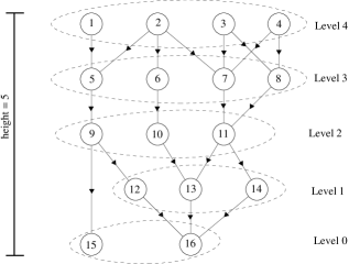
Figure 1: The height of a DAG

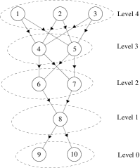
Figure 2: A level order graph

Definition 1

(Level order graph) A directed acyclic graph is a level order graph if each vertex of a given level $l$ is a predecessor of all the vertices of level $l-1$ (see Figure 2).

Series-parallel graphs (sp-graph) are defined in many ways, we use the inductive definition of Lawler (1978).

Definition 2

(sp-graph) A graph consisting of a single vertex is a sp-graph. Given two sp-graphs $G_{1}=(X_{1},A_{1})$ and $G_{2}=(X_{2},A_{2})$, the graph $G=(X_{1}\cup X_{2},A_{1}\cup A_{2})$ is a sp-graph (this is called parallel composition). Given two sp-graphs $G_{1}=(X_{1},A_{1})$ and $G_{2}=(X_{2},A_{2})$, the graph $G=(X_{1}\cup X_{2},A_{1}\cup A_{2}\cup X_{1}\times X_{2})$ is a sp-graph (this is called series composition).

An example is given in Figure 4. Note that sp-graph can also be defined by the forbidden subgraph of Figure 4.

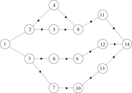
Figure 3: A series-parallel graph

Figure 4: The forbidden subgraph for sp-graphs

A divide-and-conquer-graph (DC-graph) is a special sp-graph built using symmetries. It can be used to model divide-and-conquer algorithms (for example binary search, merge sort, number multiplication…) and is formally defined as follows:

Definition 3

(DC-graph) A single vertex is a DC-graph; given two vertices $s$ and $t$ and $k$ DC-graphs $(X_{1},A_{1}),\dots,(X_{k},A_{k})$, the graph $\left(\cup_{k=1}^{n}X_{k}\cup\{s\}\cup\{t\},\cup_{k=1}^{n}\left(A_{k}\cup(s\times X_{k})\cup(X_{k}\times t)\right)\right)$ is a DC-graph.

This definition is illustrated with Figure 5.

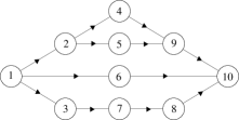
Figure 5: A DC-graph

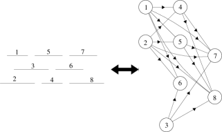
Figure 6: A set of real intervals and the corresponding interval order graph

Figure 7: The forbidden subgraph for interval order graphs

Definition 4

(Interval order graph) The interval order for a collection of intervals on the real line is the partial order corresponding to their left-to-right precedence relation, so that the interval order graph is the Hasse diagram of an interval order. such that for any two vertices $x$ and $y$, $(x,y)\in A\iff e_{x}\leq s_{y}$.

An example is given in Figure 7. Papadimitriou and Yannakakis (1979) show that interval order graphs can also be defined by the forbidden induced subgraph presented in Figure 7. Larger classes of graphs were defined by forbidden subgraphs, such as quasi-interval order graphs and over-interval order graphs (respectively in Moukrim (1999) and Chardon and Moukrim (2005)), the quasi-interval order graphs being strictly included in over-interval order graphs. The corresponding forbidden subgraphs are drawn in Figures 9 and 9.

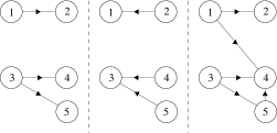
Figure 8: The three forbidden subgraphs for quasi-interval order graphs

Figure 9: The two forbidden subgraphs for over-interval order graphs

To ease the reading, the following definitions will be given within the order theory paradigm. We will hence talk about a partial order set ${\cal P}=(X,\preceq_{P})$ rather than a directed acyclic graph $G=(X,A)$ to describe the precedence graph, and a partial order $\preceq_{P}$ corresponds to the precedence constraints.

Definition 5

(Antichain) Given a partial order set ${\cal P}=(X,\preceq_{P})$, an antichain is a subset $S$ of $X$ such that any two elements of $S$ are incomparable.

Definition 6

(Width) Given a poset ${\cal P}=(X,\preceq_{P})$, the width of a poset is the size of a maximum antichain.

By extension, for a given directed acyclic graph $G=(X,A)$ we define the width of the graph to be the width of the corresponding poset, denoted by $w(G)$.

The ${\cal A}_{m}-$order (first introduced in Moukrim and Quilliot (1997)) contains the over-interval order for any integer $m\geq 2$ and is defined in the following way:

Definition 7

(${\cal A}_{m}-$order) Let ${\cal P}=(X,\preceq_{P})$ be a poset. For any two antichains $A$ and $B$ of size at most $m$, let us define the four sets : $\max(A,B)=\{x\in A\cup B|\exists y\in A\cup B,y\preceq_{P}x\}$, $\min(A,B)=\{x\in A\cup B|\exists y\in A\cup V,x\preceq_{P}y\}$, $\overline{\max}(A,B)=(A\cap B)\cup\max(A,B)$, and $\overline{\min}(A,B)=(A\cap B)\cup\min(A,B)$. $\preceq_{P}$ is an ${\cal A}_{m}$ order if and only if there do not exist two antichains $A$ and $B$ of size $m$ at most, such that $|\overline{\max}(A,B)|\geq m+1$ or $|\overline{\min}(A,B)|\geq m+1$.

We call ${\cal A}_{m}-$order graph a directed acyclic graph for which the set of arcs corresponds to an ${\cal A}_{m}-$order.

Definition 8

(Linear extension) Given a partial order $\preceq_{P}$ over a set $X$, a linear extension of $\preceq_{P}$ over $X$ is a total order respecting $\preceq_{P}$.

Definition 9

(Dimension) The dimension of a poset ${\cal P}=(X,\preceq_{P})$ is the mimimum number $t$ of linear extensions $\preceq_{1},\dots,\preceq_{t}$ such that $x\preceq_{P}y\iff\forall l\in 1..t,x\preceq_{l}y$. In other words, if $x||y$ ($x$ and $y$ are incomparable in $\preceq_{P}$), then there are at least two linear extensions, one with $x\preceq y$ and another one with $y\preceq x$.

An interesting point is that series-parallel graphs are strictly included in directed acyclic graphs of dimension 2.

The fractional dimension of a poset is extending the notion of dimension (see Brightwell and Scheinerman (1992)).

Definition 10

(Fractional dimension) For any integer $k$, $t(k)$ denotes the minimum number of linear extensions such that for any two incomparable elements $x$ and $y$, there are at least $k$ extensions with $x\preceq y$ and $k$ with $y\preceq x$. The fractional dimension is the limit $\{t(k)/k\}$ as $k$ tends to $+\infty$.

The diagram in Figure 10 provides a better overview of the existing inclusion between the different classes.

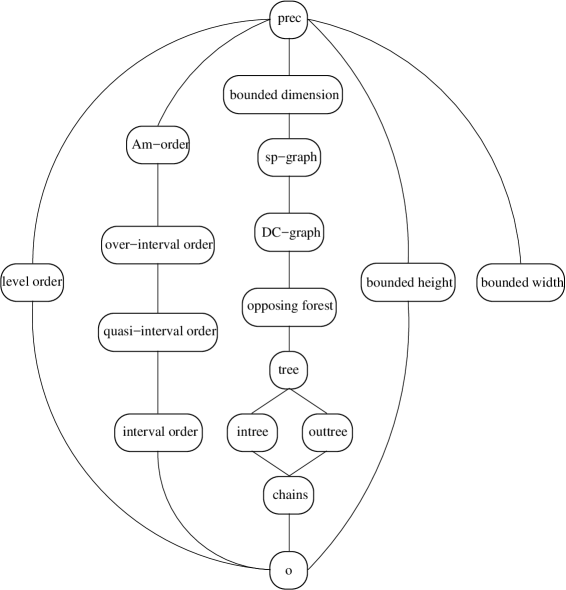
Figure 10: Hasse diagram for different classes of directed acyclic graphs

3 Scheduling notation

In this paper, we will use the standard $\alpha|\beta|\gamma$ notation introduced in Graham et al. (1979), and updated in Brucker (2007). We define below the different notations used all along the paper.

The $\alpha$-field is used for the machine environment. $\alpha=1$ corresponds to a single machine problem; if $\alpha=Pm$, there is a fixed number $m$ of identical parallel machines. If this number is arbitrary, it is noted $\alpha=P$. Similarly, if $\alpha=Qm$ (resp. $\alpha=Q$), it corresponds to a fixed (resp. arbitrary) number of uniform parallel machines, i.e., each machine $i$ has a speed $s_{i}$ and the processing time of a job $j$ on machine $i$ is equal to $p_{j}/s_{i}$.

The field $\beta\subset\{\beta_{1},\beta_{2},\beta_{3},\beta_{4}\}$ describes the jobs characteristics, the possible entries that we will deal with are the following ones:

• $\beta_{1}\in\{pmtn,\circ\}$ : $pmtn$ means that preemption is allowed, i.e., a job may be interrupted and finished later. If $\beta_{1}=\circ$, preemption is forbidden.

• $\beta_{2}$ describes the precedence constraints. If $\beta_{2}=\circ$, there is no precedence constraint, whereas $\beta_{2}=prec$ means that the precedence graph is a general directed acyclic graph. This field can take many values according to the structure of the directed acyclic graph, as presented in the previous section. For sake of completeness, all the acronyms are recalled hereinafter: $chains$, $intree$, $outtree$, $opp.forest$ (opposing forest), $io$ (interval order graph), $qio$ (quasi-interval order graph), $oio$ (over-interval order graph), $sp-graph$ (series-parallel graph), $DC-graph$ (divide-and-conquer graph), $lo$ (level order graph), $h(G)\leq k$ (directed acyclic graph with height bounded by $k$), $dim\leq k$ (directed acyclic graph with dimension bounded by $k$), $fdim\leq k$ (directed acyclic graph with fractional dimension bounded by $k$), $w(G)\leq k$ (directed acyclic graph with width bounded by $k$).

  It appears there that classical literature often abuses of terms $intree$ and $outtree$ to handle in fact $inforest$ and $outforest$, that can be mixed in $opp.forest$ for some problems.

• $\beta_{3}\in\{r_{j},\circ\}$ : if $\beta_{3}=r_{j}$, each job $j$ has a given release date. If $\beta_{3}=\circ$, the release date is $0$ for each job.

• $\beta_{4}$ represents the processing time of a job $j$. If $\beta_{4}=\circ$, there is one processing time $p_{j}$ for each job $j$. If $p_{j}=p$, all the jobs have the same processing time $p$. When $p_{j}=1$, we use the acronym UET which stands for Unit Execution Time. In some cases, the processing time may increase or decrease with either the position of the job or the starting time of the job. If the job is in position $r$ on a machine, the processing time will be noted $p_{j}^{[r]}$. If the processing time is depending of the starting time $t$ of the job, it will be written $p_{j}^{(t)}$.

The $\gamma-$field is related to the objective function of the problem. Let $C_{j}$ be the completion time of job $j$. The makespan is defined by $C_{\max}=\max_{j}C_{j}$ and the total completion time by $\sum_{j}C_{j}$. It is clear that, in general, makespan and total completion time are not equivalent. Nevertheless, for some problems, we can show that there exists an ideal schedule, which both minimizes makespan $C_{max}$ and total completion time $\sum C_{j}$. Due-date related objectives are also studied; if $d_{j}$ is the due date of job $j$, then the lateness of job $j$ is defined by $L_{j}=C_{j}-d_{j}$. The tardiness is $T_{j}=\max(0,C_{j}-d_{j})$ and the unit penalty $U_{j}$ is equal to one if $C_{j}>d_{j}$ and to zero otherwise. We then can define the maximum lateness $L_{max}=\max L_{j}$, the total tardiness $\sum T_{j}$, the total number of late jobs $\sum U_{j}$. A weight $w_{j}$ may also exist for each job $j$, leading to the corresponding objective functions: the total weighted completion time $\sum w_{j}C_{j}$, the total weighted tardiness $\sum w_{j}T_{j}$ and the total weighted number of late jobs $\sum w_{j}U_{j}$. All the functions presented so far are regular functions, i.e., they are non-decreasing with $C_{j}$.

4 Single machine problems

For single machine problems, most of the interesting results for this survey are related to the total weighted completion time $\sum w_{j}C_{j}$. It is mainly due to the fact that $1|chains,p_{j}=1|\sum U_{j}$ (see Lenstra and Rinnooy Kan (1980)) and $1|chains,p_{j}=1|\sum T_{j}$ (see Leung and Young (1990)) are already $\cal NP$-hard, while $1|prec,r_{j}|C_{\max}$ is solvable in polynomial time. Nevertheless, as we will see in Section 4.3, there are some interesting open problems for other criteria when considering preemption.

4.1 Polynomial cases

Lawler (1978) uses Sidney’s theory (Sidney (1975)) to derive a polynomial-time algorithm to solve problem $1|sp-graph|\sum w_{i}C_{i}$. The most important results are based on the concept of a module in a precedence graph $G=(N,A)$: A non-empty subset $M\subset N$ is a module if, for each job $j\in N-M$, exactly one of the three conditions holds: 1. $j$ must precede every job in $M$, 2. $j$ must follow every job in $M$, 3. $j$ is not constrained to any job in $M$. Using this concept leads to a very powerful theorem stating that there exists an optimal sequence consistent with any optimal sequence of any module.

A large improvement on this problem has been done recently, by using order theory and by proving that the problem is a special case of the vertex cover problem. More precisely, in Correa and Schulz (2005) the authors conjecture that $1|prec|\sum w_{j}C_{j}$ is a special case of vertex cover and prove that, under this conjecture, the problem $1|prec|\sum w_{j}C_{j}$ is polynomial if the precedence graph is of dimension 2. In Ambühl and Mastrolilli (2009), the authors prove the conjecture and hence the result provided in Lawler (1978) is considerably extended (since series-parallel graphs are strictly included in DAGs of dimension 2).

Using the same methodology as in Lawler (1978), Wang et al. (2008) extend these results to the case where jobs are deteriorating, i.e., processing times are an increasing function of their starting time, and they show that $1|sp-graph,p_{j}^{(t)}=p_{j}(1+at)|\sum w_{j}C_{j}$ and $1|sp-graph,p_{j}^{(t)}=p_{j}+\alpha_{j}t|C_{\max}$ can be solved in a polynomial time, where $p_{j}$, $a$, and $\alpha_{j}$ are positive constants and $t$ is the starting time of the job. The same framework is used in Wang and Wang (2013) for position-dependent processing times, and the authors show that $1|sp-graph,p_{j}^{[r]}=a_{j}+b_{j}r|C_{\max}$ and $1|sp-graph,p_{j}^{[r]}=a_{j}-b_{j}r|C_{\max}$, where $r$ is the position of the job, $a_{j}$ and $b_{j}$ positive constants, are polynomially solvable. Gordon et al. (2008) propose a more general framework than the one introduced in Wang et al. (2008), that was first presented in Monma and Sidney (1979). They extend it to different models with deterioration and learning, that were aimed at minimizing either the total weighted completion time or the makespan, with series-parallel precedence constraints.

4.2 Minimum NP-hard cases

The problem $1|prec|\sum w_{j}C_{j}$ is known to be $\cal NP$-hard (see Lenstra and Rinnooy Kan (1978)). In order to identify for which precedence graph the problem may be polynomially solvable, we present here the minimal (with respect to precedence constraints) $\cal NP$-hard cases: the problem is still ${\cal NP}-$hard even if the precedence graph is:

• of indegree at most 2 (see Lenstra and Rinnooy Kan (1978)). Note that this result also stands with equal weights (i.e., $w_{j}=1$)

• of bounded height (proof is straightforward by using the transformation proposed in Lawler (1978)).

• an interval order graph (see Ambühl et al. (2011)). This is a strong difference with parallel machine results for which interval order graphs provide often polynomial algorithms, as we will see in the dedicated section.

• of fractional dimension (see Definition 10) greater or equal to $3$ (see Ambühl et al. (2011)).

4.3 Open problems

The problem $1|prec|\sum w_{i}C_{i}$ has been widely studied, and the boundary between polynomial and $\cal NP$-hard cases is globally well-defined. However, there are still boundaries to defined, as illustrated by the following examples. First, if the fractional dimension $fdim$ of the precedence graph lies in interval $]2,3[$, the problem is open (it is polynomially solvable if $fdim\leq 2$ since the fractional dimension of a DAG is less than or equal to the dimension of this DAG and the problem is solvable in polynomial time if the precedence graph is of dimension 2). This is an interesting question but the gap is rather limited. A wider open question is when we consider the problem with equal weights, i.e., $1|prec|\sum C_{i}$. The problem is still $\cal NP$-hard, even if the precedence graph is of indegree at most 2 (see Lenstra and Rinnooy Kan (1978)). Nevertheless, we may hope that the problem becomes polynomial for precedence graphs with dimension larger than two. It is also possible that the problem is solvable in polynomial time if the precedence graph is an interval order graph, and even for larger classes like quasi-interval order graphs and over-interval order graphs.

For the criteria related to tardiness $T_{j}$ and unit penalty $U_{j}$, it is surprising to see that preemptive problems with precedence constraints have not been studied yet. More precisely, Tian et al. (2006) have shown that $1|pmtn,r_{j},p_{j}=p|\sum T_{j}$ is solvable in polynomial time, but it is still open whether adding precedence constraints leads this problem to be $\cal NP$-hard or not; the problem remains also open when considering the more general criterion $\sum w_{j}T_{j}$. The same outline appears when considering unit penalty: $1|r_{j};pmtn;p_{j}=p|\sum w_{j}U_{j}$ is solvable in polynomial time (with an algorithm in $O(n^{10})$ by Baptiste (1999), and in $O(n^{4})$ by Baptiste et al. (2004b)); nevertheless, nothing has been shown when adding precedence constraints to the problem. The first research avenue is to study this problem including Chains as a first step and determine whether the problem is polynomial or not.

5 Parallel machines without preemption

When considering non-preemptive scheduling problems, whatever the structure of precedence graphs, we will mainly focus on problems with equal processing times, since problems $P2||C_{max}$ and $P2|chains|\sum C_{j}$ are already NP-hard (see Lenstra et al. (1977) and Du et al. (1991)).

5.1 Polynomial cases

Makespan criterion and arbitrary number of machines

Three seminal works on parallel machines with precedence constraints are the approaches of Hu (1961),  Papadimitriou and Yannakakis (1979) and Möhring (1989) in which the authors are respectively dealing with trees, interval order graphs and graphs of bounded width.

In Hu (1961), the author proves that problem $P|tree,p_{j}=p|C_{\max}$ is polynomially solvable by a list scheduling algorithm where the highest priority is given to the job with the highest level (this strategy is called HLF, for Highest Level First). It is unlikely to find a precedence graph that strictly includes trees for which the problem is solvable in polynomial time, since it was proven in Garey et al. (1983) that scheduling opposing forest is $\cal NP$-hard. The hardness of the latter problem is mainly due to the arbitrary number of machines, since it is solvable in polynomial time for any fixed number of machines.

In Papadimitriou and Yannakakis (1979), the authors prove that problem $P|io,p_{j}=p|C_{\max}$ is polynomially solvable by a list scheduling algorithm where the highest priority is given to the job with the largest number of successors. This result has been improved twice; first Moukrim (1999) shows that the same algorithm gives an optimal solution if interval order graphs are replaced by quasi-interval order graphs, that properly contains the former. Chardon and Moukrim (2005) show that the same result does not stand for over-interval order graphs, but the Coffman-Graham algorithm (see Coffman Jr and Graham (1972)) can be applied to solve problem $P|oio,p_{j}=p|C_{\max}$ to optimality.

In Möhring (1989), the author studies the problem with bounded width, equal processing times and the makespan criterion. He shows that the problem can be solved in polynomial time by using dynamic programming on the digraph of order ideals. Middendorf and Timkovsky (1999) proposed their own approach to solve the problem $P|w(G)\leq k,r_{j},p_{j}=1|f$ for any regular function $f$. More precisely, their algorithm consists in searching a shortest path in the related transversal graph.

When adding release dates, the problem is already $\cal NP$-hard for intrees, yet it is solvable in polynomial time for outtrees (see Brucker et al. (1977), and Monma (1982) for a linear algorithm for the latter problem). Note that there is a strong relationship between scheduling with release dates and $C_{\max}$ criterion and scheduling with $L_{max}$, by simply looking at the schedule in the reverse way, and reversing the precedence constraints. Hence problems $P|intree,p_{j}=p|L_{max}$ is polynomially solvable and $P|outtree,p_{j}=p|L_{max}$ is $\cal NP$-hard.

Kubiak et al. (2009) recently opened new perspectives, since they show that $P|DC-graph,p_{j}=p|C_{\max}$ is solvable in polynomial time. They more precisely proved that the Highest Level First strategy (used in Hu (1961)) solves the problem to optimality when the precedence graph is a divide-and-conquer graph (see Definition 3).

Makespan criterion and fixed number of machines

Let us now focus on the case where the number of machines is fixed. Recall that the problem $Pm|prec,p_{j}=p|C_{\max}$ is still open (this problem is known as [OPEN8] in the book by Garey and Johnson (1979)) for $m\geq 3$, and it was solved for $m=2$ in Coffman Jr and Graham (1972). For opposing forests, Garey et al. (1983) propose an optimal polynomial algorithm (of complexity $O(n^{m^{2}+2m-5}\log n)$) that consists in a divide and conquer approach, that uses the HLF algorithm as a subroutine. A new algorithm with complexity $O(n^{2m-2}\log n)$ has been proposed by Dolev and Warmuth (1985), who also show that the problem is polynomially solvable for level order graphs (that are strictly included in series-parallel graphs). Dolev and Warmuth (1984) solve the case where the precedence graph is of bounded height by proposing an algorithm of time complexity $O(n^{h(m-1)+1})$. Recently, Aho and Mäkinen (2006) show that $Pm|prec,p_{j}=p|C_{\max}$ is solvable in polynomial time when the precedence graph is of bounded height and the maximum degree is bounded. This result is in fact a special case of the one proposed in Dolev and Warmuth (1984).

Other criteria and/or machine environment

The other well-studied criterion for parallel machine environment is the total completion time $\sum C_{j}$. One of the reasons for that is that, for some problems, it is equivalent to solve the total completion time and the makespan since they admit an ideal schedule. For example, ideal schedules exist when considering two machines, arbitrary precedence constraints and equal processing times, hence problem $P2|prec,p_{j}=p|\sum C_{j}$ is polynomially solvable with CG-algorithm (see Coffman Jr and Graham (1972)). When adding release dates, Baptiste and Timkovsky (2001) show that $P2|prec,r_{j},p_{j}=1|\sum C_{j}$ is solvable in polynomial time by reducing it to a shortest path problem.

For an arbitrary number of machines, if the precedence graph forms an outtree and the processing times are UET, the same result holds and hence $P|outtree,p_{j}=p|\sum C_{j}$ is solvable in polynomial time. Note that problem $P3|intree,p_{j}=p|\sum C_{j}$ is not ideal, see Huo and Leung (2006) for a counterexample. Nevertheless, for any fixed number of machines, problem $Pm|intree,p_{j}=p|\sum C_{j}$ is solvable in polynomial time (see Baptiste et al. (2004a)). Adding release dates maintains the same property: the algorithm proposed in Brucker et al. (2002) solves simultaneously problems $P|outtree,r_{j},p_{j}=1|C_{\max}$ and $P|outtree,r_{j},p_{j}=1|\sum C_{j}$. An improvement of this algorithm has been proposed in Huo and Leung (2005).

For interval order graphs, Möhring (1989) notices that $P|io,p_{j}=p|\sum C_{j}$ is solvable in polynomial time since the proof of the algorithm for $P|io,p_{j}=p|C_{\max}$ (in Papadimitriou and Yannakakis (1979)) only uses swaps between tasks, and this property is verified by the makespan and the total completion time. It has been noticed recently that the same result holds for overinterval orders (that properly contain interval orders), the problem admits also an ideal solution, so $P|oio,p_{j}=p|\sum C_{j}$ is solvable in polynomial time (see Wang (2015)).

When considering uniform parallel machines, only few results are available; problem $Q2|chains,p_{j}=p|C_{\max}$ is solvable in polynomial time (see Brucker et al. (1999)). If one processor is going $b$ times faster than the other (with $b$ an integer), the problem $Q2|tree,p_{j}=p|C_{\max}$ is also polynomially solvable (see Kubiak (1989)); the problem is also ideal, and hence $Q2|tree,p_{j}=p|\sum C_{j}$ is also solvable in polynomial time.

5.2 Minimum NP-hard cases

The interesting results for this survey are the $\cal NP$-hardness of $P|prec,p_{j}=p|C_{\max}$ and $P|prec,p_{j}=p|\sum C_{j}$ (see Lenstra and Rinnooy Kan (1978)). Note that the proof for the two problems also holds when the precedence graph is of bounded height, and that the problem $P|opp.forest,p_{j}=p|C_{\max}$ is also $\cal NP$-hard (see Garey et al. (1983)). When adding release dates, the corresponding problem is already $\cal NP$-hard for intrees, for both the makespan and the total completion time (see Brucker et al. (1977)). Finally, what may not be obvious is that even if $P||C_{max}$ is strongly $\cal NP$-hard, the problem $P|w(G)\leq k|C_{max}$ is solvable in pseudo-polynomial time (Middendorf and Timkovsky (1999)). This results is due to the fact that the class of empty graphs is not included in bounded-width graphs class.

5.3 Open problems

For an arbitrary number of machines and the makespan criterion, the boundary between polynomially solvable and $\cal NP$-hard problems seems very sharp, we believe that the efforts should not be focused on these problems. When the number of machines is fixed, this boundary is much larger. Surprisingly, to the best of our knowledge, no other structures of precedence graphs than the ones introduced in previous section have been studied for problem $P_{m}|prec,p_{j}=p|C_{\max}$. In our opinion, it could be a good opportunity to work on more general precedence graphs on this problem, to be able to arbitrate if $P_{m}|prec,p_{j}=p|C_{\max}$ is solvable in polynomial time or $\cal NP$-hard. The most natural extension in our opinion is to consider series-parallel graphs, since it is a generalization of opposing forests, level order graphs and DC-graphs, for which the problem is polynomially solvable.

For the total completion time criterion, the two most intriguing problems are $P|intree,p_{j}=p|\sum C_{j}$ and $P|outtree,r_{j},p_{j}=p|\sum C_{j}$. For the former problem, the interest lies in the fact that there exists an ideal schedule for outtree precedences, but not for intree precedences. Nevertheless, we do believe that this problem admits an optimal polynomial algorithm. For the latter problem, an algorithm exists for $p_{j}=1$ (i.e., release dates are multiple of the processing time, see Brucker et al. (2002)), and hence the gap to $p_{j}=p$ seems small.

For a fixed number of uniform parallel machines and the makespan criterion, the set of open problems is wide, since the only polynomial algorithm is for $Q2|chains,p_{j}=p|C_{\max}$ (Brucker et al. (1999)), and the problem $Qm|prec,r_{j},p_{j}=p|L_{\max}$ is still open. The same behavior occurs for the total completion time: Dessouky et al. (1990) proved that $Qm|r_{j},p_{j}=p|\sum C_{j}$ is solvable in polynomial time, and problem $Qm|prec,r_{j},p_{j}=p|\sum C_{j}$ is still open. We hence believe that this set of problems deserves a deeper study. A first approach may consist in trying to adapt the algorithms available for identical parallel machines.

6 Parallel machines with preemption

Timkovsky shows very strong links between preemption and chains, including the fact that a large set of scheduling problems with preemption can be reduced to problems without preemption, with UET tasks, and where each job is replaced by a chain of jobs (see Theorem 3.5 in Timkovsky (2003)). This interesting result can be applied in many cases, but does not hold for the total completion time criterion. Moreover, according to the structure of the precedence graph, the resulting graph may not have the same structure. For example, an intree where each job is replaced by a chain of jobs remains an intree, whereas it does not hold for interval order graphs (two independent jobs will be replaced by two chains of parallel jobs, which is not an interval order graph). That is why we will examine more precisely what happens in this section.

6.1 Polynomial cases

Makespan criterion

Since $P|tree,p_{j}=p|C_{\max}$ is polynomially solvable (see Hu (1961)), by Timkovsky’s result, so is $P|pmtn,tree|C_{\max}$. The first polynomial algorithm for this problem is proposed in Muntz and Coffman Jr (1970) with a running time of $O(n^{2})$. An algorithm in $O(n\log m)$ was then proposed in Gonzalez and Johnson (1980). Note that the latter algorithm produces at most $O(n)$ preemptions whereas the former may obtain a schedule with $O(nm)$ preemptions. Lawler (1982) studies the case with release dates and outtree, and shows that it can be solved in $O(n^{2})$ with a dynamic priority list algorithm (i.e., priorities may change according to what has already been scheduled).

Timkovsky’s result can not be applied to precedence graphs such as interval order graphs. Yet, it was proven that the problem is also solvable in polynomial time for this precedence structure; first, Sauer and Stone (1989) show it for a fixed number of machines $Pm|pmtn,io|C_{\max}$ by using a linear programming approach based on the set of jobs scheduled at each instant. Later Djellab (1999) proposes another linear program that solves the problem for an arbitrary number of machines, i.e., $P|pmtn,io|C_{\max}$. For a fixed number $m$ of machines, Moukrim and Quilliot (2005) extend the result of Sauer and Stone (1989), by proposing an linear programming approach for ${\cal A}_{m}-$order graphs (which properly contain interval order graphs).

Other criteria and/or machine environment

Du et al. (1991) explain that $P2|pmtn,chains|\sum C_{j}$ is strongly $\cal NP$-hard by showing that preemption is useless for this problem, that is why we will only focus on the UET case for the total completion time criterion. Chardon and Moukrim (2005) prove that $P2|pmtn,prec,p_{j}=p|\sum C_{j}$ is solvable in polynomial time by adapting the Coffman-Graham algorithm. Their algorithm finds an ideal schedule. By proving that preemption is redundant, Baptiste and Timkovsky (2001) prove that $P2|pmtn,outtree,r_{j},p_{j}=1|\sum C_{j}$ is solvable in polynomial time. When the precedence graph is an intree, Coffman Jr et al. (2012) prove that the problem is not ideal, and Chen et al. (2015) provide a deep analysis of the structure of preemption. Using the same methodology than Baptiste and Timkovsky (2001), Brucker et al. (2002) show that the problem is solvable in polynomial time with an outtree and an arbitrary number of machines. Moreover, they provide a $O(n^{2})$ algorithm, that admits a $O(n\log n)$ implementation according to Huo and Leung (2005). Lushchakova (2006) slightly improves the result of Baptiste and Timkovsky (2001) and proposes an algorithm of complexity $O(n^{2})$ for the problem $P2|pmtn,outtree,r_{j},p_{j}=p|\sum C_{j}$.

6.2 Minimum NP-hard cases

For the makespan criterion, Ullman (1976) shows that $P|pmtn,prec,p_{j}=p|C_{\max}$ is $\cal NP$-hard. For the total completion time criterion, if we carefully look at the $\cal NP$-hardness proof of $P|prec,p_{j}=p|\sum C_{j}$ in Lenstra and Rinnooy Kan (1978), we can see that preemption is useless for the instance constructed in the reduction and hence the preemptive version is still $\cal NP$-hard for precedence graphs of bounded height:

Theorem 1

$P|pmtn,prec,p_{j}=p|\sum C_{j}$ is $\cal NP$-hard even if the precedence graph is of bounded height.

Proof

We just need to modify slightly the proof in the reduction from Clique of Lenstra and Rinnooy Kan (1978).

Clique : $G=(V,E)$ is an undirected graph and $k$ an integer. Does $G$ have a clique on $k$ vertices?

Let us recall this reduction; we denote by $v$ (resp. $e$) the number of vertices (resp. edges) of $G$. We also define following parameters: $l=\frac{k(k-1)}{2}$, $k^{\prime}=v-k$ and $l^{\prime}=e-l$ (we use the notations of the original article). We construct an instance of $P|pmtn,prec,p_{j}=p|\sum C_{j}$ with $m=\max\{k,l+k^{\prime},l^{\prime}\}+1$ machines and $n=3m$ jobs:

• for each vertex $i\in V$, there is a job $J_{i}$.

• for each edge $[i,j]\in E$, there is a job $J_{[i,j]}$.

• dummy jobs $J_{h,t}$ with $h\in D_{t},t\in\{1,2,3\},D_{1}=\{1,\dots,m-k\},D_{2}=\{1,\dots,m-l-k^{\prime}\},D_{3}=\{1,\dots,m-l^{\prime}\}$.

There are precedence constraints between any job $J_{g,t}$ and $J_{h,t+1}$, for any $g\in D_{t},h\in D_{t+1},t=1,2$. Moreover, for any edge $[i,j]\in E$, there is a precedence between $J_{i}$ and $J_{[i,j]}$. Finally, the question is whether there is a schedule such that $\sum C_{j}\leq 6m$.

Clearly, if Clique has a solution, so is the scheduling problem:

• dummy jobs $J_{h,t}$ are scheduled during the time-interval $[t-1,t]$,

• the $k$ jobs corresponding to the vertices of the clique are scheduled during the first period,

• the $l$ jobs corresponding to the edges of the clique, and the $k^{\prime}$ jobs corresponding to the remaining vertices are scheduled at the second period,

• all the remaining jobs are scheduled at the third period.

This solution has a total completion time of exactly $6m$. Note that it does not use preemption, and is such that $C_{\max}=3$.

Conversly, let us prove that if there is a schedule such that $\sum C_{j}\leq 6m$, then there is a clique of size $k$. First, we can easily prove that if there is a schedule such that $\sum C_{j}\leq 6m$, then there is a schedule such that $C_{\max}\leq 3$. Indeed, if there exists a job $j*$ such that $C_{j*}>3$, then in the best case (i.e., if there is no precedence constraint), we have $\sum C_{j}\geq 1*m+2*m+3*(m-1)+C_{j*}>6m$. We hence know that there is no idle time and that the dummy jobs $J_{h,t}$ are scheduled during interval $[t-1,t]$. To conclude, we just need to see that if there is no clique of size $k$ then, whatever the schedule on interval $[0,1]$ without idle time, the number of eligible jobs at time $1$ is strictly less than $k^{\prime}+l$, which implies an idle time and hence no schedule such that $C_{\max}\leq 3$.

6.3 Open problems

Preemptive parallel machine scheduling problems did not receive as much attention as their non-preemptive counterpart, hence the set of open problems is wider.

For the makespan objective and an arbitrary number of machines, when the precedence graph is an interval order graph, it is known to be solvable in polynomial time, as in the UET non-preemptive case. Since for the UET non-preemptive problem, new classes strictly including interval order graphs (namely quasi-interval order graphs and over-interval order graphs) have led to polynomial algorithms, the same question arises for $P|pmtn,qio|C_{\max}$ and $P|pmtn,oio|C_{\max}$.

When the number of machines is fixed, there is a wide set of open problems, since $Qm|pmtn,prec,r_{j}|L_{\max}$ is the maximal open problem. A good challenge may be for example to try to fix the complexity of $Pm|pmtn,prec,p_{j}=p|C_{\max}$, or at least to try to find new precedence graphs for which the problem is polynomial, by taking advantage of the fact that tasks are UET (even if it may not always be helpful with preemption).

For the total completion time criterion, $P|pmtn,outtree,p_{j}=p|\sum C_{j}$ is maximal polynomially solvable, and we just show that $P|pmtn,prec,p_{j}=p|\sum C_{j}$ is $\cal NP$-hard even if the precedence graph is of bounded height. It could be interesting to consider other structures of precedence graph to derive polynomial algorithms. In a similar way, Baptiste et al. (2004a) show that $P|pmtn,p_{j}=p|\sum T_{j}$ is solvable in polynomial time, and adding precedence constraints makes the problem $\cal NP$-hard, but there is no other result available in the literature, it hence would be interesting to search for new polynomial cases by testing different precedence graphs.

For the problem $P2|pmtn,prec,r_{j},p_{j}=1|\sum C_{j}$, the gap is even wider: it is polynomial if the precedence graph is an outtree (see Baptiste and Timkovsky (2001)) but all the other cases are open, from $P2|pmtn,intree,r_{j},p_{j}=1|\sum C_{j}$ to $P2|pmtn,prec,r_{j},p_{j}=1|\sum C_{j}$.

7 Conclusion

In this paper, we surveyed the complexity results for scheduling problems with precedence constraints, and we have seen that single machine scheduling problems have been much more studied than others. This looks quite normal since the single machine problem is the scheduling problem that is the closest to order theory. Nevertheless, we show that there still are a few open problems for the single machine case. We believe that the most interesting problems for which the complexity is open lie in the parallel machine case; more precisely, we do conjecture that $Pm|sp-graph,p_{j}=p|C_{\max}$ is solvable in polynomial time; this result will be a large breakthrough since series-parallel graphs are most of the time studied for single machine problems.

Another approach to understand the complexity of scheduling problems is to deal with the parameterized complexity (see Downey and Fellows (2012)). There are only very few results on parameterized complexity of scheduling problems. One can cite Fellows and McCartin (2003) who show that, if the precedence graph is of bounded width $w$ (it is equal to the size of a maximum antichain), then problem $1|prec|\sum T_{j}\leq k$ is FPT when parameterized by $(w,k)$. The most recent result on the subject is that $P||C_{\max}$ is FPT for parameter $p_{max}=\max p_{j}$ (see Mnich and Wiese (2014)). A good graph measure is a powerful tool for parameterized complexity. For general (undirected) graphs, the creation of the treewidth (see Robertson and Seymour (1986)) helped to discover many results in graph theory, including the Courcelle’s theorem (Courcelle (1990)). For directed graphs, and more specifically DAGs, none of the existing measures (see Ganian et al. (2014)) is satisfactory. In our opinion, a major breakthrough will be achieved when one will be able to find a good measure on directed acyclic graphs.

Appendix A: List of results

For an easier reading of all the complexity results that are reviewed in this survey, we proposed a synthesis in the following tables. In each table, we write the polynomial cases, some open cases (the ones that seem the most promising in our opinion) and the $\cal NP$-hard problems.

Problem	Complexity	Reference
$1|sp-graph|\sum w_{j}C_{j}$	$\cal P$	Lawler [1978]
$1|dim\leq 2|\sum w_{j}C_{j}$	$\cal P$	Ambühl and Mastrolilli [2009]
$1|sp-graph,p_{j}^{(t)}=p_{j}(1+at)|\sum w_{j}C_{j}$	$\cal P$	Wang et al. [2008]
$1|sp-graph,p_{j}{(t)}=p_{j}+\alpha_{j}t|C_{\max}$	$\cal P$	Wang et al. [2008]
$1|sp-graph,p_{j}^{[r]}=a_{j}+b_{j}r|C_{\max}$	$\cal P$	Wang and Wang [2013]
$1|sp-graph,p_{j}^{[r]}=a_{j}-b_{j}r|C_{\max}$	$\cal P$	Wang and Wang [2013]
$1|sp-graph,p_{j}^{[r]}=p_{j}r|C_{\max}$	$\cal P$	Gordon et al. [2008]
$1|sp-graph,p_{j}^{[r]}=p_{j}\gamma^{r-1}|\sum C_{j}$ with $\gamma\geq 2$ or $0<\gamma<1$	$\cal P$	Gordon et al. [2008]
$1|sp-graph,p_{j}^{(t)}=p_{j}(1-at)|\sum w_{j}C_{j}$	$\cal P$	Gordon et al. [2008]
$1|sp-graph,p_{j}^{(t)}=p_{j}+at|\sum C_{j}$	$\cal P$	Gordon et al. [2008]
$1|sp-graph,p_{j}^{(t)}=p_{j}-at|\sum C_{j}$	$\cal P$	Gordon et al. [2008]
$1|pmtn,r_{j},p_{j}=p|\sum T_{j}$	$\cal P$	Tian et al. [2006]
$1|pmtn,r_{j},p_{j}=p|\sum w_{j}U_{j}$	$\cal P$	Baptiste [1999]
$1|2<fdim<3|\sum w_{j}C_{j}$	Open
$1|io|\sum C_{j}$	Open
$1|pmtn,chains,r_{j},p_{j}=p|\sum T_{j}$	Open
$1|pmtn,prec,r_{j},p_{j}=p|\sum w_{j}T_{j}$	Open
$1|pmtn,chains,r_{j},p_{j}=p|\sum U_{j}$	Open
$1|pmtn,prec,r_{j},p_{j}=p|\sum w_{j}U_{j}$	Open
$1|prec,p_{j}=p|\sum w_{j}C_{j}$	$\cal NP$-hard	Lawler [1978]
$1|prec|\sum C_{j}$	$\cal NP$-hard	Lawler [1978]
$1|indegree\leq 2|\sum C_{j}$	$\cal NP$-hard	Lenstra and Rinnooy Kan [1978]
$1|h(G)\leq k|\sum w_{j}C_{j}$	$\cal NP$-hard	Lawler [1978]
$1|io|\sum w_{j}C_{j}$	$\cal NP$-hard	Ambühl et al. [2011]
$1|fdim\geq 3|\sum w_{j}C_{j}$	$\cal NP$-hard	Ambühl et al. [2011]
$1|chains,p_{j}=1|\sum U_{j}$	$\cal NP$-hard	Lenstra and Rinnooy Kan [1980]
$1|chains,p_{j}=1|\sum T_{j}$	$\cal NP$-hard	Leung and Young [1990]

Table 1: Complexity results for single machine problems

Problem	Complexity	Reference
$P|tree,p_{j}=p|C_{\max}$	$\cal P$	Hu [1961]
$P|outtree,p_{j}=p|\sum C_{j}$	$\cal P$	Hu [1961]
$Pm|opp.forest,p_{j}=p|C_{\max}$	$\cal P$	Garey et al. [1983]
$Pm|lo,p_{j}=p|C_{\max}$	$\cal P$	Dolev and Warmuth [1985]
$P|io,p_{j}=p|C_{\max}$	$\cal P$	Papadimitriou and Yannakakis [1979]
$P|io,p_{j}=p|\sum C_{j}$	$\cal P$	Möhring [1989]
$P|qio,p_{j}=p|C_{\max}$	$\cal P$	Moukrim [1999]
$P|oio,p_{j}=p|C_{\max}$	$\cal P$	Chardon and Moukrim [2005]
$P|oio,p_{j}=p|\sum C_{j}$	$\cal P$	Wang [2015]
$P|outtree,r_{j},p_{j}=p|C_{\max}$	$\cal P$	Brucker et al. [1977]
$P|DC-graph,p_{j}=p|C_{\max}$	$\cal P$	Kubiak et al. [2009]
$Pm|h(G)\leq k,p_{j}=p|C_{\max}$	$\cal P$	Dolev and Warmuth [1984]
$P|w(G)\leq k,r_{j},p_{j}=1|f$	$\cal P$	Middendorf and Timkovsky [1999]
$P2|prec,p_{j}=p|C_{\max}$	$\cal P$	Coffman Jr and Graham [1972]
$P2|prec,p_{j}=p|\sum C_{j}$	$\cal P$	Coffman Jr and Graham [1972]
$P2|prec,r_{j},p_{j}=1|\sum C_{j}$	$\cal P$	Baptiste and Timkovsky [2004]
$Q2|chains,p_{j}=p|C_{\max}$	$\cal P$	Brucker et al. [1999]
$Pm|intree,p_{j}=p|\sum C_{j}$	$\cal P$	Baptiste et al. [2004a]
$P|outtree,r_{j},p_{j}=1|\sum C_{j}$	$\cal P$	Brucker et al. [2002]
$Qm|r_{j},p_{j}=p|\sum C_{j}$	$\cal P$	Dessouky et al. [1990]
$Pm|sp-graph,p_{j}=p|C_{\max}$	Open
$Pm|prec,p_{j}=p|C_{\max}$	Open
$P|intree,p_{j}=p|\sum C_{j}$	Open
$P|outtree,r_{j},p_{j}=p|\sum C_{j}$	Open
$Qm|prec,r_{j},p_{j}=p|L_{\max}$	Open
$Qm|prec,r_{j},p_{j}=p|\sum C_{j}$	Open
$P2||C_{\max}$	$\cal NP$-hard	Lenstra et al. [1977]
$P2|chains|\sum C_{j}$	$\cal NP$-hard	Du et al. [1991]
$P|opp.forest,p_{j}=p|C_{\max}$	$\cal NP$-hard	Garey et al. [1983]
$P|h(G)\leq k,p_{j}=p|C_{\max}$	$\cal NP$-hard	Lenstra and Rinnooy Kan [1978]
$P|intree,r_{j},p_{j}=p|C_{\max}$	$\cal NP$-hard	Brucker et al. [1977]
$P|h(G)\leq k,p_{j}=p|\sum C_{j}$	$\cal NP$-hard	Lenstra and Rinnooy Kan [1978]
$P|intree,r_{j},p_{j}=1|\sum C_{j}$	$\cal NP$-hard	Lenstra

Table 2: Complexity results for parallel machine problems without preemption

Problem	Complexity	Reference
$P|pmtn,tree|C_{\max}$	$\cal P$	Muntz and Coffman Jr [1970]
$P|pmtn,outtree,r_{j}|C_{\max}$	$\cal P$	Lawler [1982]
$P|pmtn,io|C_{\max}$	$\cal P$	Djellab [1999]
$Pm|pmtn,{\cal A}_{m}|C_{\max}$	$\cal P$	Moukrim and Quilliot [2005]
$P2|pmtn,outtree,r_{j},p_{j}=1|\sum C_{j}$	$\cal P$	Baptiste and Timkovsky [2001]
$P2|pmtn,outtree,r_{j},p_{j}=p|\sum C_{j}$	$\cal P$	Lushchakova [2006]
$P|pmtn,outtree,r_{j},p_{j}=1|\sum C_{j}$	$\cal P$	Brucker et al. [2002]
$P2|pmtn,prec,p_{j}=1|\sum C_{j}$	$\cal P$	Coffman et al. [2003]
$Pm|pmtn,qio,p_{j}=p|C_{\max}$	Open
$Pm|pmtn,oio,p_{j}=p|C_{\max}$	Open
$Pm|pmtn,lo,p_{j}=p|C_{\max}$	Open
$Pm|pmtn,sp-graph,p_{j}=p|C_{\max}$	Open
$Pm|pmtn,prec,p_{j}=p|C_{\max}$	Open
$Qm|pmtn,prec,r_{j}|L_{\max}$	Open
$P2|pmtn,intree,r_{j},p_{j}=1|\sum C_{j}$	Open
$P2|pmtn,prec,r_{j},p_{j}=1|\sum C_{j}$	Open
$P|pmtn,prec,p_{j}=p|C_{\max}$	$\cal NP$-hard	Ullman [1976]
$P2|pmtn,chains|\sum C_{j}$	$\cal NP$-hard	Du et al. [1991]
$P|pmtn,h(G)\leq k,p_{j}=p|\sum C_{j}$	$\cal NP$-hard	[this paper]
$P2|pmtn,chains,p_{j}=1|\sum w_{j}C_{j}$	$\cal NP$-hard	Du et al. [1991]
$P2|pmtn,chains,p_{j}=1|\sum U_{j}$	$\cal NP$-hard	Baptiste et al. [2004a]

Table 3: Complexity results for parallel machine problems with preemption

References

- Aho and Mäkinen [2006] Isto Aho and Erkki Mäkinen. On a parallel machine scheduling problem with precedence constraints. Journal of Scheduling, 9(5):493–495, 2006.