A minimal seesaw model with mu-tau symmetry

Abstract:

We analyse a flavour model for a lepton sector which is based on type I seesaw mechanism, a $\mathbbm{Z}_{2}$ symmetry for lepton flavours, a $\mu$–$\tau$ interchange symmetry and a $CP$ symmetry. This model fits well the data of neutrino mass squared differences and oscillation angles. The model predicts an overall neutrino mass scale for normal and inverted neutrino mass hierarchy and the effective mass $m_{\beta\!\beta}$, which is used in the neutrinoless double beta decay.

1 The model

Using the ideas of ref. [1] we modify the model of ref. [2]: we get neutrino masses by the type I seesaw mechanism and restrict the Lagrangian with a $\mathbbm{Z}_{2}$ symmetry for each lepton flavour and a $CP$ symmetry incorporating the interchange of two lepton flavours.

We take the lepton sector with three right-handed neutrinos and impose the three family lepton numbers $L_{e}$, $L_{\mu}$, and $L_{\tau}$. Therefore, the lepton sector comprises the multiplets $D_{eL}$, $D_{\mu L}$, $D_{\tau L}$, $e_{R}$, $\mu_{R}$, $\tau_{R}$, $\nu_{eR}$, $\nu_{\mu R}$, and $\nu_{\tau R}$. The scalar sector of the model includes three doublets:

$$\phi_{k}=\left(\begin{array}[]{c}\varphi_{k}^{+}\\[1.42262pt] \varphi_{k}^{0}\end{array}\right),\quad\tilde{\phi}_{k}=\left(\begin{array}[]{c}{\varphi_{k}^{0}}^{\ast}\\[1.42262pt] -\varphi_{k}^{-}\end{array}\right),\quad k=1,2,3.$$ (1)

In addition to the family-lepton-number symmetries we have three symmetries in the model. The first one ensures that only $\phi_{3}$ has Yukawa couplings to the electron family:

$$\mathbbm{Z}_{2}^{(e)}:\quad D_{eL}\to-D_{eL},\ \phi_{3}\to-\phi_{3}.$$ (2)

The second symmetry is the $\mu$–$\tau$ interchange symmetry

$$\mathbbm{Z}_{2}^{(\mathrm{int})}:\quad D_{\mu L}\leftrightarrow D_{\tau L},\ \mu_{R}\leftrightarrow\tau_{R},\ \nu_{\mu R}\leftrightarrow\nu_{\tau R},\ \phi_{2}\to-\phi_{2}.$$ (3)

Notice that $\phi_{2}$ changes sign under $\mathbbm{Z}_{2}^{(\mathrm{int})}$. If $\varphi_{2}^{0}$ acquires a vacuum expectation value (vev) $v_{2}$, the $\mu$–$\tau$ interchange symmetry gets broken. The third symmetry is the $CP$ symmetry

$$\begin{array}[]{rcl}&&\left\{\begin{array}[]{rcl}D_{eL}(x)&\to&\gamma_{0}C\bar{D}_{eL}^{T}(\bar{x})\\[2.84526pt] D_{\mu L}(x)&\to&\gamma_{0}C\bar{D}_{\tau L}^{T}(\bar{x})\\[2.84526pt] D_{\tau L}(x)&\to&\gamma_{0}C\bar{D}_{\mu L}^{T}(\bar{x})\end{array}\right.,\quad\left\{\begin{array}[]{rcl}e_{R}(x)&\to&\gamma_{0}C\bar{e}_{R}^{T}(\bar{x})\\[2.84526pt] \mu_{R}(x)&\to&\gamma_{0}C\bar{\tau}_{R}^{T}(\bar{x})\\[2.84526pt] \tau_{R}(x)&\to&\gamma_{0}C\bar{\mu}_{R}^{T}(\bar{x})\end{array}\right.,\\[-5.69054pt] CP:&&\\[-5.69054pt] &&\left\{\begin{array}[]{rcl}\nu_{eR}(x)&\to&\gamma_{0}C\bar{\nu}_{eR}^{T}(\bar{x})\\[2.84526pt] \nu_{\mu R}(x)&\to&\gamma_{0}C\bar{\nu}_{\tau R}^{T}(\bar{x})\\[2.84526pt] \nu_{\tau R}(x)&\to&\gamma_{0}C\bar{\nu}_{\mu R}^{T}(\bar{x})\end{array}\right.,\quad\left\{\begin{array}[]{rcl}\phi_{1}(x)&\to&\phi_{1}^{\ast}(\bar{x})\\ \phi_{2}(x)&\to&-\phi_{2}^{\ast}(\bar{x})\\ \phi_{3}(x)&\to&\phi_{3}^{\ast}(\bar{x})\end{array}\right.,\end{array}$$ (4)

where $x=\left(t,\,\vec{r}\right)$ and $\bar{x}=\left(t,\,-\vec{r}\right)$. Notice that $CP$ interchanges the $\mu$ and $\tau$ lepton flavours and that $\phi_{2}$ changes sign under $CP$.

Majorana masses of the right-handed neutrinos are generated at the (very high) seesaw scale and are given by

$$\mathcal{L}_{\mathrm{Majorana}}=-\frac{1}{2}\left(\begin{array}[]{ccc}\bar{\nu}_{eR},&\bar{\nu}_{\mu R},&\bar{\nu}_{\tau R}\end{array}\right)M_{R}\,C\left(\begin{array}[]{c}\bar{\nu}_{eR}^{T}\\ \bar{\nu}_{\mu R}^{T}\\ \bar{\nu}_{\tau R}^{T}\end{array}\right)+\mathrm{H.c.}$$ (9)

where $M_{R}$ is a $3\times 3$ symmetric matrix. These mass terms violate the family lepton numbers softly, but they are not allowed to violate neither $\mathbbm{Z}_{2}^{(\mathrm{int})}$ nor $CP$. $M_{R}$ has a typical $\mu$–$\tau$ symmetric form with real numbers.

The Yukawa couplings have the dimension four and must conserve the family lepton numbers. They are real because of the $CP$ symmetry and together with the vevs produce the Dirac mass terms of the leptons

$$\mathcal{L}_{\mathrm{Dirac}}=-\left(\begin{array}[]{ccc}\bar{e}_{L},&\bar{\mu}_{L},&\bar{\tau}_{L}\end{array}\right)M_{\ell}\left(\begin{array}[]{c}e_{R}\\ \mu_{R}\\ \tau_{R}\end{array}\right)-\left(\begin{array}[]{ccc}\bar{\nu}_{eR},&\bar{\nu}_{\mu R},&\bar{\nu}_{\tau R}\end{array}\right)\,M_{D}\left(\begin{array}[]{c}\nu_{eL}\\ \nu_{\mu L}\\ \nu_{\tau L}\end{array}\right)+\mathrm{H.c.}$$ (10)

In this model $M_{\ell}=\mathrm{diag}\left(x_{e},\,x_{\mu},\,x_{\tau}\right)$, and $M_{D}=\mathrm{diag}\left(a_{e}^{\ast},\,a_{\mu}^{\ast},\,a_{\tau}^{\ast}\right)$. The charged-lepton masses are $m_{\alpha}=\left|x_{\alpha}\right|$, where $\alpha=e,\mu,\tau$.

Using the fact that $M_{R}$ is at a much higher scale than $M_{D}$, we may use the see-saw formula to obtain the effective light-neutrino mass terms

$$\mathcal{L}_{\mathrm{light}\,\nu\,\mathrm{mass}}=\frac{1}{2}\sum_{\alpha,\beta=e,\mu,\tau}\nu_{\alpha L}^{T}\left(M_{\nu}\right)_{\alpha\beta}\nu_{\beta L}+\mathrm{H.c.},$$ (11)

where

$$M_{\nu}\approx-M_{D}^{T}M_{R}^{-1}M_{D}.$$ (12)

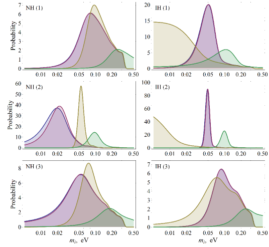
Figure 1: Distributions of the neutrino masses for the cases 1, 2, and 3 of table 1. Normal and inverted hierarchies of the neutrino masses (NH and IH) are analysed and shown on the left and right, respectively. The curves of blue, purple, and yellow colors represent the masses of the light neutrinos, $m_{1}$, $m_{2}$, and $m_{3}$, respectively. The green color indicates the distribution of $\sum m_{i}$.

The symmetries of the model, $\mathbbm{Z}_{2}^{(\mathrm{int})}$ and $CP$, lead to the following constraints on the matrix elements of $M_{\nu}$:

$$\left|M_{\nu,22}M_{\nu,13}^{2}\right|=\left|M_{\nu,33}M_{\nu,12}^{2}\right|,$$ (13a)

$$\arg{\left(M_{\nu,11}^{\ast}M_{\nu,22}^{\ast}M_{\nu,12}^{2}\right)}=\arg{\left(M_{\nu,11}^{\ast}M_{\nu,33}^{\ast}M_{\nu,13}^{2}\right)}=0\ \mathrm{or}\ \pi,\hskip 14.22636pt\arg{\left(M_{\nu,22}^{\ast}M_{\nu,33}^{\ast}M_{\nu,23}^{2}\right)}=0.$$ (13b)

This corresponds to one condition on the moduli and three conditions on the phases of the neutrino masses and mixings. The conditions (13b) mean that $M_{\nu}$ is real.

2 Numerical analysis

We write the neutrino mass matrix as

$$M_{\nu}=U^{\ast}\,\mathrm{diag}\left(m_{1},\,m_{2}e^{-i\alpha_{21}},\,m_{3}e^{-i\alpha_{31}}\right)U^{\dagger},$$ (14)

where the $m_{k}$ ($k=1,2,3$) are the neutrino masses, which are real, and $\alpha_{21}$ and $\alpha_{31}$ are the Majorana phases. The unitary matrix $U$ is parameterized like the PMNS mixing matrix [3] which contains three oscillation angles $\theta_{12},\theta_{13},\theta_{23}$ and one $CP$ violating Dirac phase $\delta$.

Since the neutrino mass matrix $M_{\nu}$ is real, the phases $\alpha_{21}$, $\alpha_{31}$, and $\delta$ may be either $0$ or $\pi$. We make eight separate numerical fits to the experimental data [4], according to the distinct values of the phases, listed in table 1. Both normal and inverted hierarchies of the light neutrino masses are considered. If the Majorana phases fulfil the condition $e^{i\alpha_{23}}=e^{i\alpha_{31}}=-1$ (cases 4 and 8), acceptable fits cannot not be obtained, but other cases yield good results.

We use the $3\sigma$ intervals for the experimental values of $\theta_{ij}$, for mass-squared difference $\Delta m_{21}^{2}=m_{2}^{2}-m_{1}^{2}$, and for $\left|\Delta m^{2}\right|=\left|m_{3}^{2}-\left.\left(m_{2}^{2}+m_{1}^{2}\right)\,\right/2\right|$ as given in ref. [4]. We impose an upper limit on the sum of the neutrino masses: $m_{1}+m_{2}+m_{3}\leq 1\,\mathrm{eV}$.

case	1	2	3	4	5	6	7	8
$e^{i\alpha_{21}}$	$+1$	$+1$	$-1$	$-1$	$+1$	$+1$	$-1$	$-1$
$e^{i\alpha_{31}}$	$+1$	$-1$	$+1$	$-1$	$+1$	$-1$	$+1$	$-1$
$e^{i\delta}$	$+1$	$+1$	$+1$	$+1$	$-1$	$-1$	$-1$	$-1$

Table 1: Values of $e^{i\alpha_{21}}$, $e^{i\alpha_{31}}$, and $e^{i\delta}$ for different cases of fits.

The plots in figs. 1, 2 and 3 present the results of numerical scans. The distributions of the neutrino masses for the cases 1, 2, and 3 look very similar to the distributions of the cases 5, 6, and 7 (according to the pattern of the Majorana phases), for both normal and inverted hierarchies. Therefore in fig. 1 we present the probability distributions of the neutrino masses only for the first three cases. Due to a small value of $\Delta m_{21}^{2}$ the distributions of the first and the second neutrino mass overlap in most cases with an exception for the case 2 assuming normal hierarchy.

The oscillation angles $\sin^{2}\theta_{12}$ and $\sin^{2}\theta_{13}$ fill our scatter plots uniformly, however, the values of $\sin^{2}\theta_{23}$ have specific probability distributions in each case of table 1. They are presented in fig. 2 for normal and inverted hierarchies.

Another quantity that we can predict is the effective mass $m_{\beta\!\beta}=|M_{ee}|$, which is related to the neutrinoless double beta decay. Figure 3 shows the relations between the sum of the neutrino masses and $|M_{ee}|$. The scatter plots for the cases 1, 2, and 3 look very similar to the plots of the cases 5, 6, and 7, for both normal and inverted hierarchies. We present only the first three cases.

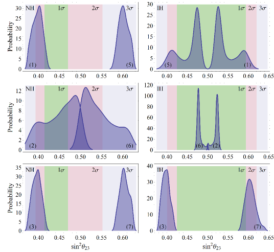
Figure 2: Distributions of the oscillation angle $\sin^{2}\theta_{23}$ for different cases of table 1. The case is indicated by a number in parantheses. Normal and inverted hierarchies of the neutrino masses (NH and IH) are shown on the left and right, respectively. The blue, red, and green colors of the background represent the $3\sigma$, $2\sigma$, and $1\sigma$ intervals of the experimental data.

Figure 3: Plots for the sum of the neutrino masses $\sum m_{i}$ vs. $m_{\beta\!\beta}=|M_{ee}|$ for the cases 1, 2, and 3 of table 1. Normal and inverted hierarchies of the neutrino masses (NH and IH) are analysed. The blue, red, and green colors of dots represent the $3\sigma$, $2\sigma$, and $1\sigma$ intervals of the experimental data. The yellow curve represents the distribution of $m_{\beta\!\beta}$. Detailed views of the densely distributed points are shown separately in the insets.

3 Summary

The model with the symmetries $\mathbbm{Z}_{2}^{(\mathrm{int})}$ and $CP$ fits well the phenomenological data for the lepton mixing angles and for the neutrino mass-squared differences. The model predicts an overall neutrino mass scale for normal and inverted neutrino mass hierarchies. When the Majorana phases are $e^{i\alpha_{21}}=+1$ and $e^{i\alpha_{31}}=-1$ (the cases 2 and 6 of table 1), the neutrino mass scale is quite low and fulfills the majority of the current cosmological bounds. The Majorana phases have a greater influence to the studied distributions than the Dirac phase. The effective mass $m_{\beta\beta}$ has its median in the interval $(0.01-0.33)$ eV, but the statistical majority of its values are distributed in the range of $0.01-0.1$ eV. The distribution of $m_{\beta\!\beta}$ is different in each analysed case.

References

[1]
P. M. Ferreira, L. Lavoura, and P. O. Ludl, Five models for lepton mixing,
J. High Energy Phys. 1308 (2013) 113 [arXiv:1304.1654].
[2]
W. Grimus and L. Lavoura, Softly broken lepton numbers and maximal neutrino mixing,
J. High Energy Phys. 0107 (2001) 045 [hep-ph/0105212].
[3]
K. A. Olive et al. (Particle Data Group),
Chin. Phys. C 38 (2014) 090001.
[4]
F. Capozzi, G. L. Fogli, E. Lisi, A. Marrone, D. Montanino, and A. Palazzo, Status of three-neutrino oscillation parameters, circa 2013,
Phys. Rev. D 89 (2014) 093018 [arXiv:1312.2878].