A geometric method for model reduction of biochemical networks with polynomial rate functions

Abstract

Model reduction of biochemical networks relies on the knowledge of slow and fast variables. We provide a geometric method, based on the Newton polytope, to identify slow variables of a biochemical network with polynomial rate functions. The gist of the method is the notion of tropical equilibration that provides approximate descriptions of slow invariant manifolds. Compared to extant numerical algorithms such as the intrinsic low dimensional manifold method, our approach is symbolic and utilizes orders of magnitude instead of precise values of the model parameters. Application of this method to a large collection of biochemical network models supports the idea that the number of dynamical variables in minimal models of cell physiology can be small, in spite of the large number of molecular regulatory actors.

1 Introduction

Model reduction is an important problem in computational biology. There are several methods for reducing networks of biochemical reactions. Formal model reduction can be based on conservation laws, exact lumping [6], and more generally, symmetry [3, 31]. Approximate numerical reduction methods, such as computational singular perturbation (CSP, [17]), intrinsic low dimensional manifold (ILDM, [20]) exploit the separation of timescales of various processes and variables. In dissipative systems, fast variables relax rapidly to some low dimensional attractive manifold called invariant manifold [8] that carries the slow mode dynamics. A projection of dynamical equations onto this manifold provides the reduced dynamics [20, 8]. This simple picture can be complexified to cope with hierarchies of invariant manifolds and with phenomena such as transverse instability, excitability and itineracy. Firstly, the relaxation towards an attractor can have several stages, each with its own invariant manifold. During relaxation towards the attractor, invariant manifolds are usually embedded one into another (there is a decrease of dimensionality) [2]. Secondly, invariant manifolds can lose local stability, which allow the trajectories to perform large phase space excursions before returning in a different place on the same invariant manifold or on a different one [14]. The set of slow variables can change from one place to another. For all these reasons, even for fixed parameters, nonlinear models can have several reductions.

CSP and ILDM methods provide numerical approximations of the invariant manifold close to an attractor. These methods have been successfully applied to reduce networks of reactions in chemical engineering. Other reduction methods utilize quasi-steady state (QSS) or quasi-equilibrium (QE) approximations [11, 28, 29]. QE and QSS methods require the knowledge of which species and reactions are fast. This knowledge can result from the slow/fast decompositions performed numerically by CSP or ILDM methods, or from the calculation of a slowness index [28], in all cases relying on trajectory simulation. The application of these methods to computational biology is possible when model parameters are known. When parameters are unknown, or if they are known only by their orders of magnitudes, formal model reduction is needed. In addition, it is convenient to find reductions without having to simulate trajectories.

In this paper we propose a fully formal method to identify the slow and fast variables in a biochemical kinetic model with polynomial rate functions, without simulation of the trajectories. The method is based on computation of tropical equilibrations. Tropical methods [19, 21], also known as idempotent or max-plus algebras due their name to the fact that one of the pioneer of the field, Imre Simon, was Brazilian. These methods found numerous applications to computer science [38], physics [19], railway traffic [1], and statistics [27]. We have shown recently that they can be used to analyse systems of polynomial or rational differential equations with applications to cell cycle modelling [25]. The main idea of our approach is to identify situations when two or several monomials of different signs equilibrate each other and dominate all the remaining monomials in the right hand side of the differential equations defining the chemical kinetics. We call this situation tropical equilibration [26]. Tropical equilibration was previously used in an interesting study by Savageau [35] as a design tool for network steady states. Our present focus is different because we are concerned with dynamics and model reduction. We also propose an algorithm using the Newton polytope to solve the tropical equilibration problem efficiently for large biochemical networks. An alternative algorithm for finding tropical equilibrations, based on constraint logic programming was proposed in [39]. However, when there are infinite branches of equilibrations, logic programming has no other alternative but the exhaustive enumeration of solutions between arbitrary bounds, whereas the Newton polytope method detects one solution per branch which is enough for identifying variable timescales and reduced models.

2 Approach

2.1 Dynamical equations and slow-fast decomposition

The biochemical networks stemming from cell biology integrate processes evolving on very different time scales. For instance, the changes of messenger RNA concentrations are usually faster compared to changes of protein concentrations and the post-transcriptional modifications of proteins (for instance phosphorylation) are faster than protein synthesis. For this reason, we will consider here slow-fast systems that have variables evolving on very different timescales. Formally, variables $\boldsymbol{x}$ are much faster than variables $\boldsymbol{y}$ if the logarithmic derivatives $\frac{\mathrm{d}\log(\boldsymbol{x})}{\mathrm{d}t}$ are much larger in absolute values than $\frac{\mathrm{d}\log(\boldsymbol{y})}{\mathrm{d}t}$. After time rescaling, the differential equations describing the dynamics of a system with fast variables $\boldsymbol{x}$ and slow variables $\boldsymbol{y}$ read as:

$$\frac{\mathrm{d}\boldsymbol{x}}{\mathrm{d}t} =\frac{1}{\eta}\boldsymbol{f}(\boldsymbol{x},\boldsymbol{y})$$ (1)

$$\frac{\mathrm{d}\boldsymbol{y}}{\mathrm{d}t} =\boldsymbol{g}(\boldsymbol{x},\boldsymbol{y}),$$ (2)

where $\eta$ is a small positive parameter and $\boldsymbol{f}$, $\boldsymbol{g}$ are functions not depending of $\eta$.

In biochemical networks, the variables $\boldsymbol{x}$ and $\boldsymbol{y}$ are (positive) species concentrations. Therefore, the functions $\boldsymbol{f}$, $\boldsymbol{g}$ are defined on the positive orthant. Furthermore, for most of the kinetic laws, the functions $\boldsymbol{f}$, $\boldsymbol{g}$ are polynomial or rational in the species concentrations. Although our methods apply for both polynomial and rational functions, for the sake of simplicity we will consider that $\boldsymbol{f}$ and $\boldsymbol{g}$ are polynomial functions. The system (1),(2) is endowed with positive initial conditions for all variables:

$$\boldsymbol{x}(0)=\boldsymbol{x}_{0},\,\boldsymbol{y}(0)=\boldsymbol{y}_{0}.$$ (3)

Let us suppose that the fast dynamics (1) has a unique stable state $\boldsymbol{x}^{*}(\boldsymbol{y})$ for all fixed $\boldsymbol{y}$ values. Let $\boldsymbol{J}(\boldsymbol{y})$ be the linear operator (Jacobian) that gives the linearization of $\boldsymbol{f}(\boldsymbol{x},\boldsymbol{y})$ at fixed $\boldsymbol{y}$, namely

$$\boldsymbol{f}(\boldsymbol{x},\boldsymbol{y})=\boldsymbol{J}(\boldsymbol{y})(\boldsymbol{x}-\boldsymbol{x}^{*}(\boldsymbol{y}))+O(|\boldsymbol{x}-\boldsymbol{x}^{*}(\boldsymbol{y})|^{2}).$$

We say that the stable state $\boldsymbol{x}^{*}(\boldsymbol{y})$ is uniformly hyperbolic if all the eigenvalues in the spectrum $Spec_{\boldsymbol{J}(\boldsymbol{y})}$ of $\boldsymbol{J}(\boldsymbol{y})$ have strictly negative real parts and are at a distance from the imaginary axis larger than a value $d>0$, namely

$${\text{ there is }d>0\text{ such that }}Re(\lambda)<-d\text{ for all }\lambda\in Spec_{\boldsymbol{J}(\boldsymbol{y})}\text{ for all }\boldsymbol{y}.$$ (4)

Tikhonov’s theorem [42] says that if the above conditions are satisfied, then after a quick transition the system evolves approximately according to the following differential-algebraic equation:

$$\frac{\mathrm{d}\boldsymbol{y}}{\mathrm{d}t}=\boldsymbol{g}(\boldsymbol{x},\boldsymbol{y}),$$ (5)

$$\boldsymbol{f}(\boldsymbol{x},\boldsymbol{y})=0.$$ (6)

More precisely, the difference between solutions of (1),(2) and solutions of (5),(6) starting from the same initial data satisfying (6) (i.e. $\boldsymbol{y}(0)=\boldsymbol{y}_{0}$, $\boldsymbol{x}(0)=\boldsymbol{x}^{*}_{0}$, where $\boldsymbol{x}^{*}_{0}$ is the unique solution of $\boldsymbol{f}(\boldsymbol{x},\boldsymbol{y}_{0})=0$) vanishes asymptotically like a positive power of $\eta$ when $\eta\to 0$. In the case when (1) has several stable steady states, then which one of these states will be chosen as solution of (6) will depend on the initial conditions (3) of the full model.

Eq. (6) means that the fast variables are slaved by the slow ones. In this case, and given the condition (4) on the Jacobian of $\boldsymbol{f}$ one can implicitly solve (6) and transform (5) into an autonomous reduced model for the slow variables. This approach is known as quasi-steady state approximation.

The first and most important step in the implementation of this reduction method is to find the slow-fast decomposition (1),(2), which means to identify $\boldsymbol{x}$, $\boldsymbol{y}$ and $\eta$. For small models this can be done by rescaling variables and kinetic constants and by identifying the small parameter $\eta$ as a ratio of kinetic constants or initial values of the variables. A well known example is the quasi-steady state approximation of the Michaelis-Menten enzymatic mechanism, when $\boldsymbol{x}$ is the concentration of the enzyme-substrate complex, $\boldsymbol{y}$ is the substrate concentration and $\eta$ represents the ratio of the enzyme to the substrate concentrations [26]. More generally, $\eta$ can be interpreted as the ratio of fast to slow timescales. Numerical methods such as ILDM [20] use the Jacobian of the full system to obtain the slow-fast decomposition. In such methods $\eta$ can be interpreted as the gap separating in logarithmic scale, the timescales of slow and fast variables obtained from the spectrum of the Jacobian. In this paper we present a symbolic method to perform the same decomposition. This method is based on tropical geometry [19, 21].

2.2 Tropical equilibrations and timescales of the variables

We consider biochemical networks described by the following differential equations

$$\frac{\mathrm{d}x_{i}}{\mathrm{d}t}=\sum_{j\in[1,r]}k_{j}{S_{ij}}\boldsymbol{x}^{\boldsymbol{\alpha_{j}}},\,i\in[1,n].$$ (7)

where $k_{j}>0,j\in[1,r]$ are kinetic constants, $r$ is the number of reactions, $S_{ij}$ are the elements of the so-called stoichiometric matrix, $\boldsymbol{\alpha}_{j}=(\alpha_{1}^{j},\ldots,\alpha_{n}^{j})\in{\mathbb{Z}}^{n}_{+}$ are multi-indices, $\boldsymbol{x^{\boldsymbol{\alpha}_{j}}}=x_{1}^{\alpha_{1}^{j}}\ldots x_{n}^{\alpha_{n}^{j}}$ and $x_{i},\,i\in[1,n]$ are the species concentrations, $n$ being the number of species.

The polynomial equations (7) can result from the mass action law. For instance, a reaction $A+B\to C$ of kinetic constant $k$ and satisfying the mass action law, has $S_{11}=-1,S_{21}=-1,S_{31}=1$, $\boldsymbol{\alpha}_{1}=(1,1,0)$, which correspond to the kinetic equations

$$\frac{\mathrm{d}x_{1}}{\mathrm{d}t} =-kx_{1}x_{2},$$

$$\frac{\mathrm{d}x_{2}}{\mathrm{d}t} =-kx_{1}x_{2},$$

$$\frac{\mathrm{d}x_{3}}{\mathrm{d}t} =kx_{1}x_{2},$$ (8)

where $x_{1}$, $x_{2}$, $x_{3}$ are the concentrations of $A$, $B$, $C$, respectively.

We can notice that the mass action law implies tight relations between $\alpha_{j}$ and $S_{ij}$, namely $\alpha_{i}^{j}=-S_{ij}$ if $S_{ij}<0$, otherwise $\alpha_{i}^{j}=0$. These relations are not needed in our approach. Furthermore, our method can be extended to the more general case when reaction rates are rational functions of the concentrations. Typically, we can use the least common denominator of reaction rates to express the right hand sides of the kinetic equations as ratios of polynomials and apply the method to the numerators. This extension was briefly discussed in [25].

In what follows, the kinetic parameters do not have to be known precisely and they are given by their orders of magnitude. Usually, orders of magnitude are approximations of the parameters by integer powers of ten and serve for rough comparisons. Our definition of orders of magnitude is based on the equation

$$k_{j}=\bar{k}_{j}\varepsilon^{\gamma_{j}},\quad\gamma_{j}=\text{round}(\log(k_{j})/\log(\varepsilon)),$$ (9)

where $\varepsilon$ is a positive parameter smaller than $1$, $\gamma_{j}$ is the order of $k_{j}$, $\bar{k}_{j}$ has order zero and round stands for the closest integer, with half-integers rounded to even numbers. When $\epsilon=1/10$, our definition provides the usual decimal orders. Parameter order calculation is the first step of the algorithm in Sect. 3.1.

We must emphasize that the parameter $\varepsilon$ introduced in this section is not necessarily the fast/slow timescale ratio $\eta$ occurring in Tikhonov’s theorem. As a matter of fact, as will be shown later in this section, the parameter $\eta$ can be expressed as a power of $\varepsilon$. In short, $\varepsilon$ is used just for expressing everything as powers.

From (9) it follows that if $\gamma_{j}\neq\gamma_{i}$ and $\gamma_{i}$ are integers, then $k_{i}/k_{j}>1/\varepsilon{>>1}$ or $k_{j}/k_{i}>1/\varepsilon{>>1}$, meaning that the parameters $k_{i}$, $k_{j}$ are well separated. However, the condition $\gamma_{j}\neq\gamma_{i}$ is not always needed in this approach. All we need is the separation between the slow and fast timescales resulting from our calculations (this will be the gap condition introduced later in this section). Networks with well separated constants were also studied in [9] for the particular case of monomolecular reactions.

Timescales of nonlinear systems depend not only on parameters but also on species concentrations, which are a priori unknown. In order to compute them, we introduce a vector $\boldsymbol{a}=(a_{1},\ldots,a_{n})$, such that

$$\boldsymbol{x}=\bar{\boldsymbol{x}}\varepsilon^{\boldsymbol{a}}.$$ (10)

The orders $a_{i}$ are generally rational and can be positive or negative. Of course, negative orders $a_{i}<0$ do not mean negative concentrations, but very large concentrations, because $\varepsilon<1$. In general, a higher $a_{i}$ means a smaller concentration $x_{i}$.

Orders $\boldsymbol{a}$ are unknown and have to be calculated. To this aim, the network dynamics can be described by a rescaled ODE system

$$\frac{\mathrm{d}\bar{x}_{i}}{\mathrm{d}t}=(\sum_{j}\varepsilon^{\mu_{j}}\bar{k}_{j}{S_{ij}}{\bar{\boldsymbol{x}}}^{\boldsymbol{\alpha_{j}}})\varepsilon^{-a_{i}},$$ (11)

where $\mu_{j}=\gamma_{j}+\langle\boldsymbol{a},\boldsymbol{\alpha_{j}}\rangle,$ and $\langle,\rangle$ stands for the vector dot product.

The r.h.s. of each equation in (11) is a sum of multivariate monomials in the concentrations. The exponents $\mu_{j}$ indicate how large are these monomials, in absolute value. Generically, one monomial of exponent $\mu_{j}$ dominates the others $\mu_{j}<\mu_{j^{\prime}},j^{\prime}\neq j$. Accordingly, variables under the influence of a single dominant monomial, undergo large changes in a short time. The interesting case is when all variables are submitted to two dominant forces, one positive and one negative and these forces have the same order. We call this situation tropical equilibration ([26]). More precisely, we have the following

Definition 2.1

We call tropical equilibration solutions the vectors $\boldsymbol{a}\in{\mathbb{R}}^{n}$ for which the minimum in the definition of the piecewise-affine function ${\psi}_{i}(\boldsymbol{a})=\min_{j}(\gamma_{j}+\langle\boldsymbol{a},\boldsymbol{\alpha_{j}}\rangle)$ is attained for at least two indices $j^{\prime},j^{\prime\prime}$ corresponding to opposite signs monomials, i.e. $S_{ij^{\prime}}S_{ij^{\prime\prime}}<0$. Equivalently, a tropical equilibration is a solution of the following system of equations for the orders $\boldsymbol{a}$:

$$\min_{j,S{ij}<0}(\gamma_{j}+\langle\boldsymbol{a},\boldsymbol{\alpha_{j}}\rangle)=\min_{j^{\prime},S{ij^{\prime}}>0}(\gamma_{j}+\langle\boldsymbol{a},\boldsymbol{\alpha_{j}}\rangle),\quad i=1,\ldots,n.$$ (12)

For instance, if $\frac{\mathrm{d}{x}_{1}}{\mathrm{d}t}=\bar{k}_{1}x_{1}x_{2}-\varepsilon^{1}\bar{k}_{2}x_{1}+\varepsilon^{2}\bar{k}_{3}x_{2}$, we have $\psi_{1}(\boldsymbol{a})=\min\{a_{1}+a_{2},1+a_{1},2+a_{2}\}$. Tropical equilibrations are solutions of $\min\{a_{1}+a_{2},2+a_{2}\}=1+a_{1}$, equivalent to $a_{1}+a_{2}=1+a_{1}\leq 2+a_{2}$ or $2+a_{2}=1+a_{1}\leq a_{1}+a_{2}$.

Intuitively, tropical equilibration means that dominant forces on variables compensate each other and that variables change slowly under the influence of the remaining weak forces. Compensation of dominant forces constrains the dynamics of the system to a low dimensional invariant manifold [25, 29, 26].

Tropical equilibrations are used to calculate the unknown orders $\boldsymbol{a}$ as solutions of the system (12). The solutions of (12) have a geometrical interpretation. Let us define the extended order vectors $\boldsymbol{a}^{e}=(1,\boldsymbol{a})\in{\mathbb{R}}^{n+1}$ and extended exponent vectors $\boldsymbol{\alpha}_{j}^{e}=(\gamma_{j},\boldsymbol{\alpha}_{j})\in{\mathbb{Z}}^{n+1}$. Let us consider the equality $\mu_{j}=\mu_{j^{\prime}}$. This represents the equation of a $n$ dimensional hyperplane of ${\mathbb{R}}^{n+1}$, orthogonal to the vector $\boldsymbol{\alpha_{j}}^{e}-\boldsymbol{\alpha_{j^{\prime}}}^{e}$:

$$\langle\boldsymbol{a}^{e},\boldsymbol{\alpha_{j}}^{e}\rangle=\langle\boldsymbol{a}^{e},\boldsymbol{\alpha_{j^{\prime}}}^{e}\rangle,$$ (13)

where $\langle,\rangle$ is the dot product in ${\mathbb{R}}^{n+1}$. We will see in the next section that the minimality condition on the exponents $\mu_{j}$ implies that the normal vectors $\boldsymbol{\alpha_{j}}^{e}-\boldsymbol{\alpha_{j^{\prime}}}^{e}$ are edges of the so-called Newton polytope [15, 40]. The algorithmic way to solve the set of inequalities in Eq. 12 along with the sign condition is described in Sects. 3.2, 3.3.

We call tropically truncated system the system obtained by pruning the system (11), i.e. by keeping only the dominating monomials.

$$\frac{\mathrm{d}\bar{x}_{i}}{\mathrm{d}t}=\varepsilon^{\nu_{i}}(\sum_{j\in{D(i)}}\bar{k}_{j}S_{ij}{\bar{\boldsymbol{x}}}^{\boldsymbol{\alpha_{j}}}),$$ (14)

where ${D(i)}=\underset{j}{\operatorname*{\arg\!\min}}(\mu_{j},S_{ij}\neq 0)$ selects the dominating rates of reactions acting on species $i$ and

$$\nu_{i}=\min\{\mu_{j}|S_{ij}\neq 0\}-a_{i}.$$ (15)

The tropically truncated equations contain generically two monomial terms of opposite signs (in special cases they can contain more than two terms among which two have opposite signs). Polynomial systems with two monomial terms are called binomial or toric. In systems biology, toric systems are known as S-systems and were used by Savageau [34] for modeling metabolic networks.

The truncated system (14) indicates how fast is each variable, relatively to the others. The inverse timescale of a variable $x_{i}$ is given by $\frac{1}{x_{i}}\frac{\mathrm{d}x_{i}}{\mathrm{d}t}=\frac{1}{\bar{x}_{i}}\frac{\mathrm{d}\bar{x}_{i}}{\mathrm{d}t}$ that scales like $\varepsilon^{\nu_{i}}$. Thus, if $\nu_{i^{\prime}}<\nu_{i}$ then $x_{i^{\prime}}$ is faster than $x_{i}$.

Let us assume that $\nu_{1}\leq\nu_{2}\leq\ldots\leq\nu_{n}$ (this may require species re-indexing but is always possible) and the following gap condition is fulfilled:

$$\text{there is }m<n\text{ such that }\nu_{m+1}-\nu_{m}>0,$$ (16)

meaning that two groups of variables have separated timescales. The variables $\boldsymbol{X}_{r}=(x_{1},x_{2},\ldots,x_{m})$ are fast (change significantly on timescales of order of magnitude $\varepsilon^{-\nu_{m}}$ or shorter). The remaining variables $\boldsymbol{X}_{s}=(x_{m+1},x_{m+2},\ldots,x_{n})$ are slow (have little variation on timescales of order of magnitude $\varepsilon^{-\nu_{m}}$). Then, the parameter $\eta=\varepsilon^{\nu_{m+1}-\nu_{m}}$ represents the fast/slow timescale ratio in the Tikhonov’s theorem from the preceding section. Our gap condition means that $\eta$ should be small. With these conditions, we have shown in [26, 30] that quasi-steady state approximation can be applied. A further complication arises when the system has fast cycles and this will be described in the next section.

For systems with hierarchical relaxation, the separation between fast and slow variables is mobile within the cascade of relaxing modes. In the extreme case this means that all the species timescales are distinct and separated by large enough gaps. Let us consider that we are interested in changes on timescales $\theta$ or slower. The timescale $\theta$ defines a threshold order value by the equation

$$\mu_{\text{threshold}}=-\log(\theta/\tau)/\log(\varepsilon),$$ (17)

where $\tau$ are the time units from the model. Then, from (14) it follows that all variables $x_{i}$ with $\nu_{i}\geq\mu_{\text{threshold}}$ are slow. Perturbations in the concentrations of these species relax to an attractor slower or as slow as $\theta$. The remaining species are fast and the perturbations in their concentrations relax to equilibrated values much faster than $\theta$.

2.3 Model reduction of fast cycles

Tropical truncation is useful for identifying the slow and fast variables of a system of polynomial differential equations. However, the truncation alone is not always enough for accurate reduction. As discussed in [26, 30], there are situations when the truncated system is not a good approximation. Typically, truncation could eliminate all the reactions exiting a fast cyclic subnetwork. Thus we get new conserved quantities, that were not conserved by the full model. Truncation is in this case accurate at short times, but introduces errors at large times. In order to cope with fast cycles pruning, we adopt the recipe discussed in [11] for the quasi-equilibrium approximation. This recipe allows one to recover the terms that were neglected by truncation, but which are important for large time dynamics.

First, let us remind some definitions. We call linear conservation law of a system of differential equations, a linear form $C(\boldsymbol{x})=<\boldsymbol{c},\boldsymbol{x}>=c_{1}x_{1}+c_{2}x_{2}+\ldots+c_{n}x_{n}$ that is identically constant on trajectories of the system. It can be easily checked that vectors in the left kernel $Ker^{l}(S)$ of the stoichiometric matrix $\boldsymbol{S}$ provide linear conservation laws of the system (7). Indeed, system (7) reads $\frac{\mathrm{d}\boldsymbol{x}}{\mathrm{d}t}=\boldsymbol{S}\boldsymbol{R}(\boldsymbol{x})$, where the components of the vector $\boldsymbol{R}$ are $R_{j}(\boldsymbol{x})=k_{j}x^{\alpha_{j}}$. If $\boldsymbol{c}\boldsymbol{S}=0$, then $\frac{\mathrm{d}<\boldsymbol{c},\boldsymbol{x}>}{\mathrm{d}t}=\boldsymbol{c}\boldsymbol{S}\boldsymbol{R}(\boldsymbol{x})=0$, where $\boldsymbol{c}=(c_{1},c_{2},\ldots,c_{n})$.

Let us assume that the truncated system (14), restricted to the fast variables has a number of independent, linear conservation laws, defined by the left kernel vectors $\boldsymbol{c}_{1},\boldsymbol{c}_{2},\ldots,\boldsymbol{c}_{d}$, where $\boldsymbol{c}_{k}=(c_{k1},c_{k2},\ldots,c_{kf})$. These conservation laws can be calculated by recasting the truncated system as the product of a new stoichiometric matrix and a vector of monomial rate functions and further computing left kernel vectors of the new stoichiometric matrix. We further assume that the fast conservation laws are not conserved by the full system (7).

We define the new slow variables $\boldsymbol{Y}=(y_{1},\ldots,y_{d})$, where $y_{k}=\sum_{i=1}^{f}c_{ki}x_{i}$. and eliminate the fast variables $x_{1},x_{2},\ldots,x_{f}$ by using the system :

$$\sum_{j\in{D(i)}}k_{j}S_{ij}{\boldsymbol{x}}^{\boldsymbol{\alpha_{j}}} = 0,\,i\in[1,f],$$ (18)

$$\sum_{i=1}^{f}c_{ki}x_{i} = y_{k},\,k\in[1,d].$$ (19)

Reactions of the initial model that were pruned by truncation have to be restored if they act on the new slow variables $\boldsymbol{Y}$, i.e. if $\sum_{i=1}^{f}c_{li}S_{ik}\neq 0$, for some $l\in[1,d]$, where $k$ is the index of the reaction to be tested. Finally, the kinetic laws of these reactions have to be redefined in terms of the slow variables $\boldsymbol{X}^{s},\boldsymbol{Y}$.

The rigourous justification of the reduction procedure for models with fast cycles can be found in [30].

3 Algorithm to compute tropical equilibrations.

In this section we introduce an algorithm allowing the automatic computation of tropical equilibrations.

3.1 Pre-processing

We consider examples with polynomial vector field. The kinetic parameters of the equation system are scaled based on Eq. (9).

3.2 Newton polytope and edge filtering

For each equation and species $i$, we define a Newton polytope ${\mathcal{N}}_{i}\subset{\mathbb{R}}^{n+1},$ that is the convex hull of the union of all the half-lines emanating in the positive $\epsilon$ direction from the points $\alpha_{j}$ such that $S_{ij}\neq 0$ (thus, we first consider these half-lines and then take their convex hull). This is the Newton polytope of the polynomial in right hand side of Eq. (11), with the scaling parameter $\varepsilon$ considered as a new variable. If $\varepsilon$ does not appear in the coefficients of Eq. (11), then the half-lines above are replaced by the origins $\alpha_{j}$. The Newton polytope is in this case the convex hull of the points $\alpha_{j}$ such that $S_{ij}\neq 0$.

As explained in Sect. 2.2 the tropical equilibrations correspond to vectors $\boldsymbol{a}^{e}=(1,\boldsymbol{a})\in{\mathbb{R}}^{n+1}$ satisfying the optimality condition of Definition 12. This condition is satisfied automatically on hyperplanes orthogonal to edges of Newton polytope connecting vertices $\boldsymbol{\alpha}_{j^{\prime}}^{e}$, $\boldsymbol{\alpha}_{j^{\prime\prime}}^{e}$ satisfying the opposite sign condition. Therefore, a subset of edges from Newton polytope is selected based on the filtering criteria which tells that the vertices belonging to an edge should be from opposite sign monomials as explained in Eq. (20).

$$E(P)=\{\{v_{1},v_{2}\}\subseteq\left({}_{2}^{V}\right)\mid\text{conv}(v_{1},v_{2})\in F_{1}(P),$$

$$\wedge\,\text{sign}(v_{1})\times\text{sign}(v_{2})=-1\},$$ (20)

where $v_{i}$ is the vertex of the polytope and $V$ is the vertex set of the polytope, $\text{conv}(v_{1},v_{2})$ is the convex hull of vertices $v_{1},v_{2}$ and $F_{1}(P)$ is the set of 1-dimensional face (edges) of the polytope. $\text{sign}(v_{i})$ represents the sign of the monomial which corresponds to vertex $v_{i}$.

Fig. 1 shows an example of Newton polytope construction for a single equation $\dot{x}_{1}=-x_{1}^{6}+x_{1}^{3}x_{2}-x_{1}^{3}+x_{1}x_{2}^{2}$. Cf. definition 12 and eq.(12) tropical equilibrations are solutions of the equation

$$\min(3a_{1}+a_{2},a_{1}+2a_{2})=\min(6a_{1},3a_{1}).$$

Using a brute force method, tropical equilibration can be computed by solving the system

$$\text{case 1: }3a_{1}+a_{2}=3a_{1},\,3a_{1}+a_{2}\leq a_{1}+2a_{2},\,3a_{1}\leq 6a_{1},$$ (21)

$$\text{case 2: }3a_{1}+a_{2}=6a_{1},\,3a_{1}+a_{2}\leq a_{1}+2a_{2},\,3a_{1}\geq 6a_{1},$$ (22)

$$\text{case 3: }a_{1}+2a_{2}=3a_{1},\,3a_{1}+a_{2}\geq a_{1}+2a_{2},\,3a_{1}\leq 6a_{1},$$ (23)

$$\text{case 4: }a_{1}+2a_{2}=6a_{1},\,3a_{1}+a_{2}\geq a_{1}+2a_{2},\,3a_{1}\geq 6a_{1}.$$ (24)

The Newton polytope construction simplifies this task by automatically eliminating some of the cases (21),(22),(23),(24). We start by associating a point in the $n$-dimensional space (here a plane, because there are two variables, $n=2$) to each monomial of the polynomial equation. In Fig. 1 the points $(6,0)$, $(3,1)$, $(3,0)$, $(1,2)$, correspond to the monomials $x_{1}^{6}$, $x_{1}^{3}x_{2}$, $x_{1}^{3}$, $x_{1}x_{2}^{2}$, respectively. The Newton polytope is the convex hull of the set of these points and has four vertices (the point $(3,1)$ corresponding to the monomial $x_{1}^{3}x_{2}$ is internal to the polytope). Each pair of points corresponding to monomials that have opposite signs in the original differential equation indicates the choice of one of the four cases (21),(22),(23),(24). For instance Case 1 means choosing the pair of points $(3,1)$ and $(3,0)$. The Newton polytope construction allows one to identify the cases involving internal points as redundant or impossible and to eliminate them.

Indeed, it can be easily checked that the cases 1 and 2 (Eqs.(21),(22)) have only the trivial solution $a_{1}=a_{2}=0$ that is also solution of cases 3 and 4.

Case 3 corresponds to the choice of the points $(1,2)$ and $(3,0)$ that are vertices of the Newton polytope. The solution of (23) is $a_{1}=a_{2}\geq 0$ and describes a half line orthogonal to the edge of the Newton polytope connecting the vertices $(1,2)$ and $(3,0)$.

Case 4 follows from the choice of the vertices $(1,2)$ and $(6,0)$. It has the solution $2a_{2}=5a_{1}\leq 0$ that describes a half line orthogonal to the corresponding edge of the Newton polytope.

Further definitions and full proofs of the properties of a Newton polytope can be found in [15, 40].

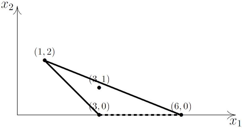
Figure 1: An example of a Newton polytope for the polynomial $-x_{1}^{6}+x_{1}^{3}x_{2}-x_{1}^{3}+x_{1}x_{2}^{2}$. In this example, the monomial coefficients do not depend on $\varepsilon$ and we want to solve the tropical problem $\min(3a_{1}+a_{2},a_{1}+2a_{2})=\min(6a_{1},3a_{1})$. The Newton polytope vertices $(6,0),(3,0),(1,2)$ are connected by lines. The point $(3,1)$ is not a vertex as it lies in the interior of the polytope. This stems to having $\min(3a_{1}+a_{2},a_{1}+2a_{2})=a_{1}+2a_{2}$ for all tropical solutions, which reduces the number of cases to be tested. The thick edges satisfy the sign condition, whereas the dashed edge does not satisfy this condition. For this example, the solutions of the tropical problem are in infinite number and are carried by the two half-lines $a_{1}=a_{2}\geq 0$ and $5a_{1}=2a_{2}\leq 0$, orthogonal to the thick edges of the Newton polygon.

3.3 Pruning and feasible solutions

We formalize here the pruning procedure illustrated for the simple example of the previous subsection.

By feasible solution we understand a vector $(a_{1},\ldots,a_{n})$ satisfying all the equations of the system (12). A feasible solution lies in the intersection of hyperplanes (or convex subsets of these hyperplanes) orthogonal to edges of Newton polytopes obeying the sign conditions. Of course, not all sequences of edges lead to nonempty intersections and thus feasible solutions. This can be tested by the following linear programming problem, resulting from (12):

$$\begin{split}\gamma_{j}(i)+\langle\boldsymbol{a},\boldsymbol{\alpha_{j}(i)}\rangle=\gamma_{j^{\prime}}(i)+\langle\boldsymbol{a},\boldsymbol{\alpha_{j^{\prime}}(i)}\rangle\leq\gamma_{j^{\prime\prime}}+\langle\boldsymbol{a},\boldsymbol{\alpha_{j^{\prime\prime}}}\rangle),\\ \text{for all}\,j^{\prime\prime}\neq j,j^{\prime},{S_{ij^{\prime\prime}}\neq 0},\quad i=1,\ldots,n,\end{split}$$ (25)

where $j(i),j^{\prime}(i)$ define the chosen edge of the $i-$th Newton polytope. The set of indices $j^{\prime\prime}$ can be restricted to vertices of the Newton polytope, because the inequalities are automatically fulfilled for monomials that are internal to the Newton polytope. For instance, for the example of the preceding section, the choice of the edge connecting vertices $(1,2)$ and $(3,0)$ leads to the following linear programming problem:

$$a_{1}+2a_{2}=3a_{1}\leq 6a_{1},\,{3a_{1}+a_{2}\geq a_{1}+2a_{2}},$$

whose solution is a half-line orthogonal to the edge of the Newton polygon.

We introduce a pruning methodology (similar to a branch and bound algorithm technique) which helps to reduce the number of possible choices of Newton polytope edges leading to feasible solutions. Let us consider a system of polynomial equations and order the equations as $eq_{1},eq_{2},...,eq_{n}$. Let the vertices of Newton polytope ${\mathcal{N}}_{n}$ be $v_{n1},v_{n2},...,v_{nl}$ where $l$ is the total number of vertices. The polytope edges are described by $ne_{1},ne_{2},...,ne_{n}$ where $ne_{i}$ denotes the set of edges from Newton polytope ${\mathcal{N}}_{i}$. In order to search for feasible solutions an edge from each polytope needs to be selected. This translates to evaluating the cartesian product of $ne_{1},ne_{2},\ldots,ne_{n}$ which can be described by the following equation

$$ne_{1}\times ne_{2}\times...\times ne_{n}=\{(e_{1j},e_{2j},...,e_{nj})\mid(e_{1j}$$

$$\in ne_{1})\wedge(e_{2j}\in ne_{2})\wedge...\wedge(e_{nj}\in ne_{n})\}.$$ (26)

where $e_{nj}$ is the $j^{th}$ edge in Newton polytope ${\mathcal{N}}_{n}$. It is clear from the above that the possible choices are exponential. In order to improve the running time of the algorithm, the pruning strategy evaluates Eq. (26) in several steps(cf. Algorithm 1 and Fig. 2). It starts with an arbitrary pair of edges and proceeds to add the next edge only when the inequalities (25) restricted to these two pair of edges are satisfied. The corresponding set of inequalities can be solved using any standard linear programming package.

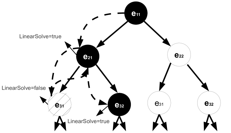
Figure 2: Pruning strategy. This figure explains the pruning technique described in Sect. 3.3 and the evaluation of Eq. (26).The possible combinations of edges are represented in a tree representation. The algorithm starts by testing for feasible solution for first pair of edge sets. If a feasible solution is found, the algorithm proceeds further to other edge sets or it backtracks. In the figure, $e_{11}$ and $e_{21}$ are selected from edge sets $ne_{1}$, $ne_{2}$ and are checked for a feasible solution satisfying (25). If such a solution exists, it moves to $e_{31}$from the next edge set and again checks for feasible solution, if not then it backtracks to $e_{21}$ and then to $e_{32}$ which results in a feasible solution. Therefore, the sub-tree with root node $e_{31}$ is discarded from future searches and this improves running time. Likewise the branch $e_{11}$ and $e_{22}$ is explored. This approach is similar to branch and bound algorithm technique. The dashed arrows show the flow of the program.

Input: List of edge sets $ne_{1},ne_{2},...,ne_{n}$, and the corresponding vertices

Output: Orders of the variables $\boldsymbol{a}_{1},\boldsymbol{a}_{2},...,\boldsymbol{a}_{n}$ (tropical equilibration solution set)

1 begin

2       solutionset ={}; integer $k$=1; equation = {} SolveOrders(equation, $k$, edge-sets, vertices) if $k>n$ then

3             return

4      for $l=1$ to number of entries in $ne_{k}$edge-set do

5             equation(k)* = vertices in $l^{th}$row inequalities* = all other vertices in $ne_{1}$to $ne_{k}$edge-sets if  LinearSolve(equation,inequalities)is feasible then

6                   if  $k=n$  then

7                        add the solution of LinearSolve to solutionset

8                  SolveOrders(equation, $k+1$, $ne_{1},..,ne_{k}$, vertices)

9            

10      

11

*The equations and inequalities are initialised as per Eq. (25)

Algorithm 1 SolveOrders: Steps of tropical equilibration algorithm

3.4 Examples

As an illustration of our method we have chosen simple models that (i) have polynomial dynamics and (ii) contain fast cycles that ask for the reduction steps described in Sect.2.3. The Michaelis-Menten model of enzymatic reactions as well as a cell cycle model proposed by Tyson [43] satisfy both these conditions.

3.4.1 The Michaelis-Menten model

The irreversible Michaelis-Menten kinetics consist of three reactions:

$$S+E\underset{k_{-1}}{\overset{k_{1}}{\rightleftharpoons}}ES\overset{k_{2}}{\rightarrow}P+E,$$

where $S,ES,E,P$ represent the substrate, the enzyme-substrate complex, the enzyme and the product, respectively.

The corresponding system of polynomial differential equations reads:

$$\begin{split}\dot{x}_{1}&=-k_{1}x_{1}x_{3}+k_{-1}x_{2},\\ \dot{x}_{2}&=k_{1}x_{1}x_{3}-(k_{-1}+k_{2})x_{2},\\ \dot{x}_{3}&=-k_{1}x_{1}x_{3}+(k_{-1}+k_{2})x_{2},\\ \dot{x}_{4}&=k_{2}x_{2},\end{split}$$ (27)

where $x_{1}=[S]$, $x_{2}=[ES]$, $x_{3}=[E]$, $x_{4}=[P]$.

The system (27) has two conservation laws $x_{2}+x_{3}=e_{0}$ and $x_{1}+x_{2}+x_{4}=s_{0}$. The values $e_{0}$ and $s_{0}$ of the conservation laws result from the the initial conditions, namely $e_{0}=x_{2}(0)+x_{3}(0)$ and $s_{0}=x_{1}(0)+x_{2}(0)+x_{4}(0)$.

The conservation laws can be used to eliminate the variables $x_{3}$ and $x_{4}$ and obtain the reduced system as follows

$$\begin{split}\dot{x}_{1}&=-k_{1}x_{1}(e_{0}-x_{2})+k_{-1}x_{2},\\ \dot{x}_{2}&=k_{1}x_{1}(e_{0}-x_{2})-(k_{-1}+k_{2})x_{2}.\end{split}$$ (28)

There are two types of approximations and reductions for the Michaelis-Menten model, the quasi-steady state and the quasi-equilibrium approximation [22, 36, 37, 11, 12]. We discuss here how these approximations can be related to tropical equilibrations (see also [26, 39] where the same model is analysed using tropical curves).

Let us introduce orders of variables and parameters as follows $x_{i}=\bar{x}_{i}\epsilon^{a_{i}}$, $1\leq i\leq 2$, $k_{1}=\bar{k}_{1}\epsilon^{\gamma_{1}}$, $k_{-1}=\bar{k}_{-1}\epsilon^{\gamma_{-1}}$, $e_{0}=\bar{e}_{0}\epsilon^{\gamma_{e}}$.

Then, we get the tropical equilibration equations by equating minimal orders of positive monomials with minimal orders of negative monomials in (28):

$$\gamma_{1}+\gamma_{e}+a_{1} =\min(\gamma_{1}+a_{1},\gamma_{-1})+a_{2},$$ (29)

$$\gamma_{1}+\gamma_{e}+a_{1} =\min(\gamma_{1}+a_{1},\min(\gamma_{-1},\gamma_{2}))+a_{2}.$$ (30)

The quasi-equilibrium approximation corresponds to the case when the reaction constant $k_{-1}$ is much faster than the reaction constant $k_{2}$. In terms of orders, this condition reads $\gamma_{-1}<\gamma_{2}$. In this case, the two tropical equilibration equations (29), (30) are identical, because $\min(\gamma_{-1},\gamma_{2})=\gamma_{-1}$. Let $\gamma_{m}=\gamma_{-1}-\gamma_{1}$ denote the order of the parameter $K_{m}=k_{-1}/k_{1}$. There are two branches of solutions of (29), namely $a_{2}=\gamma_{e},a_{1}\leq\gamma_{m}$ and $a_{2}=a_{1}+\gamma_{e}-\gamma_{m},a_{1}\geq\gamma_{m}$ corresponding to $\min(\gamma_{1}+a_{1},\gamma_{-1})=\gamma_{1}+a_{1}$ and to $\min(\gamma_{1}+a_{1},\gamma_{-1})=\gamma_{-1}$, respectively. Using the relation between orders and concentrations we identify the first branch of solutions with the saturation regime $x_{2}\approx e_{0}$ (the free enzyme is negligible) and $x_{1}>>K_{m}$ (the substrate has large concentration) and the second branch with the linear regime $x_{2}<<e_{0}$ (the concentration of the attached enzyme is negligible) and $x_{1}<<K_{m}$ (the substrate has low concentration).

In the linear regime of quasi-equilibrium the fast truncated system (obtained after removing all dominated monomials from (28)) reads

$$\begin{split}\dot{x}_{1}&=-k_{1}x_{1}e_{0}+k_{-1}x_{2},\\ \dot{x}_{2}&=k_{1}x_{1}e_{0}-k_{-1}x_{2}.\end{split}$$ (31)

The variable $y=x_{1}+x_{2}$ is conserved by the fast truncated system (31), but not by the full system (28). Therefore, $y$ has to be considered as a new slow variable. By summing the two equations of (28) term by term we get

$$\dot{y}=-k_{2}x_{2}.$$ (32)

Using the quasi-equilibrium equation $-k_{1}x_{1}e_{0}+k_{-1}x_{2}=0$ we eliminate $x_{1}$, $x_{2}$ by expressing them as $x_{1}=y/(1+k_{1}e_{0}/k_{-1})$, $x_{2}=y/(1+k_{-1}/(k_{1}e_{0}))$. Finally, we get the reduced model for the slow variable $y$,

$$\dot{y}=-k_{2}y/(1+k_{-1}/(k_{1}e_{0}))=-V_{max}y/(e_{0}+K_{m}),$$ (33)

where $V_{max}=k_{2}e_{0}$.

If we express $\dot{y}$ as a function of the substrate concentration $x_{1}$ we obtain $\dot{y}=-(V_{max}/K_{m})x_{1}$, which is the well known Michaelis-Menten reaction rate in the linear regime.

In the saturated quasi-equilibrium regime, the fast truncated system reads

$$\begin{split}\dot{x}_{1}&=-k_{1}x_{1}(e_{0}-x_{2}),\\ \dot{x}_{2}&=k_{1}x_{1}(e_{0}-x_{2}).\end{split}$$ (34)

From (34) we get the quasi-equilibrium equation $x_{2}=e_{0}$ and further, using (32), we find the reduced model

$$\dot{y}=-V_{max}.$$ (35)

The tropical method also allows us to test that variables $x_{1}$, $x_{2}$ are faster than $y$, which means that the reductions are consistent (fast variables are eliminated and the reduced model is written in the slow variables only). In terms of $\nu$ orders defined by eq.(15), one has to check that $\nu_{1}<\nu_{y}$ and $\nu_{2}<\nu_{y}$. Using eq.(15) together with the quasi-equilibrium condition, we find that $\nu_{2}=\gamma_{-1}$ in the linear regime and $\nu_{2}=\gamma_{1}+a_{1}$ in the saturated regime. Furthermore, $\nu_{1}\leq\gamma_{-1}+a_{2}-a_{1}$, $\nu_{y}=\gamma_{2}+a_{2}-\min(a_{1},a_{2})$ for both regimes. The condition $\nu_{1}<\nu_{y}$ is satisfied because $\gamma_{2}>\gamma_{-1}$. $\nu_{2}<\nu_{y}$ is satisfied in the linear regime because $\gamma_{2}>\gamma_{-1}$. The same condition is satisfied also in the saturated regime because $a_{1}\leq\gamma_{m}=\gamma_{-1}-\gamma_{1}$ in this regime.

To summarize, the unique condition for quasi-equilibrium is $\gamma_{2}>\gamma_{-1}$. In particular, this approximation does not depend on the initial data because $\gamma_{e}$ does not occur in the above condition.

The quasi-steady state approximation corresponds to the situation when $x_{2}$ is equilibrated and faster than $x_{1}$. In this case one has to combine (30) with the condition $\nu_{2}<\nu_{1}$. Let us denote by $\gamma_{m}=\min(\gamma_{-1},\gamma_{2})-\gamma_{1}$ the order of the parameter $K_{m}=(k_{-1}+k_{2})/k_{1}$. Eq.(30) alone has two branches of solutions. The first branch is defined by $a_{1}\leq\gamma_{m}$, $a_{2}=\gamma_{e}$ and corresponds to the saturated regime of quasi-steady state. The second branch is defined by $a_{1}\geq\gamma_{m}$, $a_{2}=a_{1}+\gamma_{e}-\gamma_{m}$ and corresponds to the linear regime. From (28) we find $\nu_{1}=\min(\gamma_{1}+a_{1}+\gamma_{e},\gamma_{1}+a_{1}+a_{2},\gamma_{-1}+a_{2})-a_{1}$ and $\nu_{2}=\gamma_{1}+a_{1}+\gamma_{e}-a_{2}$. By elementary inequality algebra it follows that the condition $\nu_{2}<\nu_{1}$ is equivalent to $a_{1}<\gamma_{e}$ at saturation and to $\gamma_{m}<\gamma_{e}$ in the linear regime.

Summarizing, the conditions for quasi-steady state are $a_{1}<\min(\gamma_{m},\gamma_{e})$ (saturation) or $\gamma_{m}<\min(a_{1},\gamma_{e})$ (linear regime). In contrast to quasi-equilibrium, quasi-steady state depends on the initial conditions.

The quasi-steady state equations at saturation are $k_{1}x_{1}(e_{0}-x_{2})=0$, leading to $x_{2}=e_{0}$. In the linear regime one has $k_{1}x_{1}e_{0}-(k_{-1}+k_{2})x_{2}=0$, leading to $x_{2}=e_{0}x_{1}/K_{m}$. Using (32) we get the well known expressions $\dot{y}=-k_{2}e_{0}=-V_{max}$ and $\dot{y}=-V_{max}x_{1}/K_{m}$ representing the reaction rate in the saturated and linear regimes, respectively.

The timescales of variables and the validity of quasi-steady state for Michaelis-Menten irreversible kinetics were previously derived by Segel [36, 37]. Our time scales and conditions are compatible with the ones of Segel on pieces, i.e. in the linear and in the saturated regime of quasi-steady state. For instance, like in [36] our conditions imply that quasi-steady state can be valid for small $\gamma_{e}$ (large enzyme) provided that $\gamma_{m}$ is smaller (very large $K_{m}$).

3.4.2 The cell cycle model

This model describes the interaction between cyclin and cyclin-dependent kinase cdc2 during the progression of the eukaryotic cell cycle (see Fig. 3). Cyclin (variable $x_{5}$) is synthesized during interphase stage of the cycle (reaction of constant $k_{6}$). Newly synthesized cyclin forms a complex with the phosphorylated kinase cdc2 (cdc2 is the variable $x_{2}$ and the complex formation reaction has constant $k_{4}$). The resulting complex (variable $x_{4}$) is called inactive or pre-maturation promoter factor (pre-MPF). pre-MPF needs to be activated for enter into mitosis in order to phosphorylate many substrates controlling processes essential for nuclear and cellular division. The active form of MPF (variable $x_{3}$) is produced from pre-MPF either by a non-regulated transformation (reaction of constant $k_{10}$) or by an autocatalytic process (reaction of constant $k_{9}$). At the end of mitosis the active complex dissociates (reaction of constant $k_{1}$), resulting in the phosphorylated cyclin (variable $x_{6}$) that is degraded (reaction of constant $k_{8}$) and the de-phosphorylated kinase cdc2 (variable $x_{1}$). The kinase is equilibrated with its phosphorylated form (variable $x_{2}$) by phosphorylation and dephosphorylation reactions (of constants $k_{2}$ and $k_{3}$ respectively).

The full model has a stable periodic attractor, a limit cycle. The stable limit cycle oscillations correspond to the periodic succession of interphase and mitosis phases of the cell cycle.

The corresponding system of differential equations along with conservation laws for the above model can be described as

$$\dot{x}_{1} = k_{1}x_{3}-k_{2}x_{1}+k_{3}x_{2},\,\dot{x}_{2}=k_{2}x_{1}-k_{3}x_{2}-k_{4}x_{2}x_{5},$$

$$\dot{x}_{3} = k_{10}x_{4}-k_{1}x_{3}+k_{9}x_{3}^{2}x_{4},$$

$$\dot{x}_{4} = k_{4}x_{2}x_{5}-k_{10}x_{4}-k_{9}x_{3}^{2}x_{4},\,\dot{x}_{5}=k_{6}-k_{4}x_{2}x_{5},$$

$$\dot{x}_{6} = k_{1}x_{3}-k_{8}x_{6},\,x_{1}+x_{2}+x_{3}+x_{4}=1.$$ (36)

The value of the conservation law $x_{1}+x_{2}+x_{3}+x_{4}=1$ follows from the initial conditions $\boldsymbol{x}(0)=(0,0.75,0,0.25,0,0)$ that were taken from [43]. Other initial conditions with the same value of the conservation law would lead to the same tropical equilibration solutions.

Applying Definition 12 and eq.(12) to this model, we obtain the following tropical equilibration problem:

$$\min(a_{3}+\gamma_{1},a_{2}+\gamma_{3})=a_{1}+\gamma_{2},$$

$$a_{1}+\gamma_{2}=\min(a_{2}+\gamma_{3},a_{2}+a_{5}+\gamma_{4}),$$

$$\min(a_{4}+\gamma_{10},2a_{3}+a_{4}+\gamma_{9})=a_{3}+\gamma_{1},$$

$$a_{2}+a_{5}+\gamma_{4}=\min(a_{4}+\gamma_{10},2a_{3}+a_{4}+\gamma_{9}),$$

$$\gamma_{6}=a_{2}+a_{5}+\gamma_{4},$$

$$a_{3}+\gamma_{1}=a_{6}+\gamma_{8},\min(a_{1},a_{2},a_{3},a_{4})=0.$$ (37)

Using the numerical values of the parameters from the original paper we find, for $\varepsilon=1/9$, $\gamma_{1}=0$, $\gamma_{2}=-6$, $\gamma_{3}=-3$, $\gamma_{4}=-2$, $\gamma_{6}=2$, $\gamma_{8}=0$, $\gamma_{9}=-2$, $\gamma_{10}=2$ (cf. Eq. 9 and Sect. 3.1).

Remark: One may notice that the orders $\gamma$ depend on which units were used for the parameters. However, if the parameter units are changed, the set of tropical equilibrations is transformed into an equivalent one. Indeed, the model equations should be invariant with respect to units conversion. In particular, if units of second order reaction constants (i.e. coefficients of second order monomial rates) are multiplied by $k$, one should subtract $log(k)/log(\varepsilon)$ from the parameter orders and add the same quantity to the concentration orders. This will generate an equivalent set of solutions, up to rounding errors.

Using our algorithm (cf. Sects.3.2, 3.3) we got three tropical equilibrations for this system, namely $\boldsymbol{a}_{1}=(8,5,2,0,-1,2)$, $\boldsymbol{a}_{2}=(5,2,2,0,2,2)$, $\boldsymbol{a}_{3}=(3,0,2,0,4,2)$.

The rescaled truncated system for the solution $\boldsymbol{a}_{3}$ reads

$$\dot{\bar{x}}_{1}=\varepsilon^{-6}(\bar{k}_{3}\bar{x}_{2}-\bar{k}_{2}\bar{x}_{1}),\dot{\bar{x}}_{2}=\varepsilon^{-3}(\bar{k}_{2}\bar{x}_{1}-\bar{k}_{3}\bar{x}_{2}),$$

$$\dot{\bar{x}}_{3}=\bar{k}_{10}\bar{x}_{4}-\bar{k}_{1}\bar{x}_{3}+\bar{k}_{9}\bar{x}_{3}^{2}\bar{x}_{4},$$

$$\dot{\bar{x}}_{4}=\varepsilon^{2}(-\bar{k}_{10}\bar{x}_{4}+\bar{k}_{4}\bar{x}_{2}\bar{x}_{5}-\bar{k}_{9}\bar{x}_{3}^{2}\bar{x}_{4}),$$

$$\dot{\bar{x}}_{5}=\varepsilon^{-2}(\bar{k}_{6}-\bar{k}_{4}\bar{x}_{2}\bar{x}_{5}),\dot{\bar{x}}_{6}=\bar{k}_{1}\bar{x}_{3}-\bar{k}_{8}\bar{x}_{6}.$$ (38)

It appears clearly that the variables $x_{1}$, $x_{2}$, $x_{5}$ are fast. More precisely, their characteristic times are $\nu_{1}^{-1}=\varepsilon^{6}$, $\nu_{2}^{-1}=\varepsilon^{3}$, $\nu_{5}^{-1}=\varepsilon^{2}$, respectively. The largest of these timescales is here approximately $0.01$ (in minutes which are the time units of the model). The remaining slow variables have characteristic times from $\varepsilon^{0}$ to $\varepsilon^{-2}$, i.e. approximately from $1$ to $100$ min. Therefore, the timescales of slow and fast species are separated by a gap, and the singular perturbation small parameter (cf. Sect.2.1) is $\eta=t_{fast}/t_{slow}\sim\varepsilon^{2}$ (the power 2 arises as the difference between $\nu_{6}=\nu_{3}=0$, coming from the fastest slow species and $\nu_{5}=-2$, coming from the slowest fast species).

The fast truncated system reads

$$\dot{x}_{1}=k_{3}x_{2}-k_{2}x_{1},\dot{x}_{2}=k_{2}x_{1}-k_{3}x_{2},$$

$$\dot{x}_{5}=k_{6}-k_{4}x_{2}x_{5}.$$ (39)

and has a single conservation law $C_{1}=x_{1}+x_{2}$ that provides a new slow variable. This conservation law, not conserved by the full system (36), indicates the presence of a fast cycle in the model. It is the rapid phosphorylation/dephosphorylation cycle transforming the cyclin $x_{1}$ into its phosphorylated form $x_{2}$ and back. The fast variables are eliminated from the system obtained by adding to (39) the definition of the fast conservation law cf. Sect.2.3:

$$k_{3}x_{2}-k_{2}x_{1}=0,k_{6}-k_{4}x_{2}x_{5}=0,y=x_{1}+x_{2}.$$ (40)

The differential equation for $y$ is obtained by adding the first two equations of the full system (36), and thus restoring the terms $k_{1}x_{3}$ and $k_{4}x_{2}x_{5}$, that have order $\varepsilon^{2}$ and were pruned in the first step.

Finally, we obtain the following reduced model

$$\dot{x}_{3}=k_{10}x_{4}-k_{1}x_{3}+k_{9}x_{3}^{2}x_{4},$$ (41)

$$\dot{x}_{4}=-k_{10}x_{4}+k_{6}-k_{9}x_{3}^{2}x_{4},$$ (42)

$$\dot{x}_{6}=k_{1}x_{3}-k_{8}x_{6},\dot{y}=k_{1}x_{3}-k_{6}.$$ (43)

and the slaved fast variables are given by $x_{1}=yk_{2}/(k_{2}+k_{3})\approx yk_{2}/k_{3}$, $x_{2}=yk_{3}/(k_{2}+k_{3})\approx y$, $x_{5}=k_{6}(k_{2}+k_{3})/(k_{4}k_{3}y){\approx k_{6}/(k_{4}y)}$, where we have used (40) and the fact that $k_{2}\ll k_{3}$.

Let us note that the variable $y$ has the same order as $x_{2}$ ($a_{y}=a_{3}=2$), it is tropically equilibrated ($\gamma_{1}+a_{3}=\gamma_{6}=2$ in Eq.(43)), and has $\nu_{y}=\gamma_{6}-a_{y}=0$ meaning that it is slow.

Let us call this four variables model reduced model 1. Note that in this model the dynamics of the variables $x_{3},x_{4}$ is decoupled from the two others. We can therefore conclude that by our approach we obtain a two dimensional minimal cell cycle model.

Repeating the procedure for the equilibrations $\boldsymbol{a}_{1}$, $\boldsymbol{a}_{2}$ we find two other rescaled truncated systems.

The rescaled truncated system for the solution $\boldsymbol{a}_{1}$ reads

$$\dot{\bar{x}}_{1}=\varepsilon^{-6}(\bar{k}_{3}\bar{x}_{2}-\bar{k}_{2}\bar{x}_{1}+k_{1}x_{3}),\dot{\bar{x}}_{2}=\varepsilon^{-3}(\bar{k}_{2}\bar{x}_{1}-\bar{k}_{3}\bar{x}_{2}),$$

$$\dot{\bar{x}}_{3}=\bar{k}_{10}\bar{x}_{4}-\bar{k}_{1}\bar{x}_{3}+\bar{k}_{9}\bar{x}_{3}^{2}\bar{x}_{4},$$

$$\dot{\bar{x}}_{4}=\varepsilon^{2}(-\bar{k}_{10}\bar{x}_{4}+\bar{k}_{4}\bar{x}_{2}\bar{x}_{5}-\bar{k}_{9}\bar{x}_{3}^{2}\bar{x}_{4}),$$

$$\dot{\bar{x}}_{5}=\varepsilon^{3}(\bar{k}_{6}-\bar{k}_{4}\bar{x}_{2}\bar{x}_{5}),\dot{\bar{x}}_{6}=\bar{k}_{1}\bar{x}_{3}-\bar{k}_{8}\bar{x}_{6},$$ (44)

and for the solution $\boldsymbol{a}_{2}$ we got

$$\dot{\bar{x}}_{1}=\varepsilon^{-6}(\bar{k}_{3}\bar{x}_{2}-\bar{k}_{2}\bar{x}_{1}),\dot{\bar{x}}_{2}=\varepsilon^{-3}(\bar{k}_{2}\bar{x}_{1}-\bar{k}_{3}\bar{x}_{2}),$$

$$\dot{\bar{x}}_{3}=\bar{k}_{10}\bar{x}_{4}-\bar{k}_{1}\bar{x}_{3}+\bar{k}_{9}\bar{x}_{3}^{2}\bar{x}_{4},$$

$$\dot{\bar{x}}_{4}=\varepsilon^{2}(-\bar{k}_{10}\bar{x}_{4}+\bar{k}_{4}\bar{x}_{2}\bar{x}_{5}-\bar{k}_{9}\bar{x}_{3}^{2}\bar{x}_{4}),$$

$$\dot{\bar{x}}_{5}=(\bar{k}_{6}-\bar{k}_{4}\bar{x}_{2}\bar{x}_{5}),\dot{\bar{x}}_{6}=\bar{k}_{1}\bar{x}_{3}-\bar{k}_{8}\bar{x}_{6}.$$ (45)

In both cases, the variable $x_{5}$ is slow, which was not the case for the equilibration $\boldsymbol{a}_{1}$. This is possible, because for a nonlinear model, the timescale of a variable depends on the concentration range in which the model functions. The equilibrations $\boldsymbol{a}_{1}$ and $\boldsymbol{a}_{2}$ correspond to very low and low concentrations of phosphorylated kinase $x_{2}$ (proportional to $\varepsilon^{5}$ and $\varepsilon^{2}$, respectively), meaning slow consumption of the cyclin $x_{5}$. The concentration of $x_{2}$ is large for the equilibration $\boldsymbol{a}_{3}$ (proportional to $\varepsilon^{0}$) leading to rapid consumption of $x_{5}$ (see Eq.(36)).

The two tropical equilibrations $\boldsymbol{a}_{1}$ and $\boldsymbol{a}_{2}$ lead to the same reduced model, which we call reduced model 2:

$$\dot{x}_{3}=k_{10}x_{4}-k_{1}x_{3}+k_{9}x_{3}^{2}x4,$$

$$\dot{x}_{4}=-k_{10}x_{4}+k_{6}-k_{9}x_{3}^{2}x_{4},$$

$$\dot{x}_{5}=k_{6}-k_{4}yx_{5},$$

$$\dot{x}_{6}=k_{1}x_{3}-k_{8}x_{6},\dot{y}=k_{1}x_{3}-k_{6},$$ (46)

to be considered together with $x_{1}=yk_{2}/k_{3}$, $x_{2}=y$.

The tropical setting confirms ideas from the theory of nonlinear dynamical systems. The two reduced models are nested. Reduced model 2 has a larger number of slow (relaxing) variables than reduced model 1. This means that the corresponding invariant manifolds are embedded one into another with the lowest dimensional one defined by the reduced model 1 carrying the dynamics on the limit cycle attractor. Starting with initial low concentrations of the phosphorylated kinase corresponding to the equilibration $\boldsymbol{a}_{1}$ or $\boldsymbol{a}_{2}$, the system will increase these concentrations to levels corresponding to the equilibration $\boldsymbol{a}_{3}$ that allow the stable limit cycle oscillations.

One can notice that our reduced model 1 does not contain the parameters $k_{2}$, $k_{3}$, $k_{4}$ of the full model. This means that as long as the phosphorylation and the dephosphorylation of the free kinase, as well as the formation of cyclin kinase complex are fast enough, the actual values of the kinetic constants of these processes are not important.

In his paper, Tyson [43] also proposes a two variables reduced model:

$$\dot{u} = k_{9}(v-u)(\alpha+u^{2})-k_{1}u,$$

$$\dot{v} = k_{6}-k_{1}u,$$ (47)

where $u=x_{3}$, $v=x_{3}+x_{4}+x_{5}$, $\alpha=k_{10}/k_{9}$.

It can be easily checked that Eqs.(47) are equivalent with our Eqs.(41),(42), provided that $x_{5}\ll x_{4}$ and $x_{5}\ll x_{3}$. These last conditions, justified by intuitive arguments, were used in the derivation of the reduced model in [43]. In our approach, the same conditions follow immediately from the orders of the species concentrations. Indeed, for the equilibration $\boldsymbol{a}_{3}$ we have $x_{5}\sim\varepsilon^{4}$, $x_{3}\sim\varepsilon^{2}$, $x_{4}\sim\varepsilon^{0}$, therefore $x_{5}\ll x_{4}$ and $x_{5}\ll x_{3}$. To summarize, the advantage of our approach is that it is automatic and can be applied to larger models that are more difficult or impossible to grasp by simple intuition.

Full model

Reduced model

Figure 3: Graphic representation of the full cell cycle model [43] (referenced as BIOMD00000005 by Biomodels) and of the reduced model 1. The full model describes the cyclin production and complex formation between the cyclin and the kinase cdc2, the autocatalytic activation (by dephosphorylation), and the dissociation of this complex followed by the destruction of the cyclin. The reduced model represents accurately the same processes, on the invariant manifold containing the periodic attractor. The different variables mean: $x_{1}:\,\text{cdc2}$, $x_{2}:\,\text{cdc2-P}$, $x_{3}:\,\text{cdc2}:\text{cyclin-P}$ i.e. active MPF complex, $x_{4}:\,\text{P-cdc2}:\text{cyclin-P}$ i.e. pre-MPF complex, $x_{5}:\,\text{cyclin}$, $x_{6}:\,\text{cyclin-P}$, $y=x_{1}+x_{2}:\,\text{total free cdc2}$. Both full and reduced model are biochemical networks with polynomial rate functions.

4 Results

4.1 Details on the implementation of the algorithm

The differential equation system along with the conservation laws for a given biochemical model (in SBML format) are generated using the pocab software[32]. Polymake [7] is used to compute the Newton polytope from the set of exponent vectors. For solving the linear programming we used Gurobi[13] in Java programming environment. The expressions in the equation system are processed using computer algebra system Maple.

4.2 Results on Biomodels database

Biological models were selected from r25 version of Biomodels [18]. For our analysis, we selected models with polynomial kinetics. We performed two analyses. (i) First, we benchmarked our implementation against models derived from Biomodels. (ii) Second, we computed the average number of slow variables across Biomodels with different time thresholds to get an estimate of the dimension of the invariant manifold.

In the first analysis, the parameters were replaced by the orders of magnitude according to Eq. (9). A summary of the analysis is presented in Table 1. The analysis is performed to compute all possible combinations of vertices leading to tropical solutions within a maximal running time of $10,000$ seconds of CPU time. The CPU time threshold for models with $\varepsilon$ value = $1/5$ was further increased to $100,000$ to further ascertain the exponential behaviour. In practice, we restrict this search space using the tree pruning strategy as explained in Sect. 3.3. While solving the linear inequalities it may happen that there exists infinite feasible solutions for a given combination of vertices. In such a scenario we report only one solution. The analysis was repeated with ten different values for $\varepsilon$. A semilog time-plot is presented in Fig. 4 which plots the log of running time in milliseconds versus the number of equations in the model. It should be pointed out that the number of variables may not be equal to the number of equations because of conservation laws which were treated as extra linear equations in our framework.

In the second analysis, the number of slow variables were computed based on the rescaled orders i.e. $\mu_{i}-a_{i}>\mu_{\text{threshold}}$ and a certain time threshold as explained in Eq. (17). In addition to slow species, we computed the quasi buffered species which are slow variables with very high time threshold. To compute them we fixed the timescale threshold to $100,000$ seconds and the slow species at this threshold are labeled as quasi buffered species. In the model, such species are practically constant and in our setting these are subtracted from slow variables. A boxplot is shown in Fig. 5 where a point represents the compression ratio (i.e. ratio of average number of slow variables / total number of variables) over all the tropical equilibrations for each model with respect to different time thresholds. This was performed for all the models under consideration. We also computed the slowest timescale for each model which is defined as the smallest time threshold at which all species become fast (the quasi-buffered species were removed from the model before performing this step). A histogram showing the distribution slowest timescale is presented in Fig. 5. To estimate the slowest timescale, the time threshold is varied and the number of slow species are counted, the threshold at which all species become fast is considered to be the slowest timescale of that model. This histogram indicates that the benchmarked models are representative of a wide variety of cellular processes whose timescales range from fractions of seconds to one day.

The calculations in this section were performed for different values of the parameter $\varepsilon$. According to the Eq.(12) and to the geometric interpretation of tropical equilibrations from Sect.2.2 the tropical solutions are either isolated points or bounded or unbounded polyhedra. Changing the parameter $\varepsilon$ is just a way to approximate the position of these points and polyhedra by lattices or in other words by integer coefficients vectors. The approximation results from the rounding in Eq.(9) and better approximations would be to consider rational (with a largest common denominator), instead of integer orders $\gamma_{i}$. Finding the value of $\varepsilon$ that provides the best approximation is a complicated problem in Diophantine approximation. For that reason, we preferred an experimental approach consisting in choosing several values of $\varepsilon$ and checking the robustness of the results.

Table 1: Summary of analysis on Biomodels database. Tropical solutions here mean existence of at least one feasible solution from all possible combination of vertices of the Newton polytope (in case of infinite solutions, one is picked (cf. Sect. 4.2)). Timed-out means all solutions could not be computed within $10,000$ seconds of computation time (except for models with $\varepsilon$ value = $1/5$). No tropical solution implies no possible combination of vertices could be found resulting in a feasible solution. Unit-definition refers to the presence of SBML tag $<$unitDefinition$>$ which defines the time units of the model to be used in Eq. (17). For the models where it is absent seconds is taken to be the default time unit of the model, with the exception of two models whose units have been curated manually by comparison with original papers.

$\varepsilon$ value	Total models considered	Timed-out models	Models without tropical solutions	Models with tropical solutions	Average running time (in secs)**	Models with Unit-definition
1/5*	53	14	0	39	1354.91	12
1/7	53	17	0	36	512.07	12
1/9	53	17	0	36	432.54	12
1/11	53	16	0	37	756.66	12
1/19	53	18	2	33	1063.30	12
1/23	53	18	1	34	783.98	12
1/47	53	18	0	35	719.79	12
1/53	53	19	0	34	387.16	12
1/59	53	19	1	33	482.30	12
1/71	53	19	0	34	640.32	12

*For this $\varepsilon$ the running time threshold was $100,000$ secs. ** For average time computation, the running times of those models which did not timed-out (i.e. $4$th and $5$th column) were considered.

Figure 4: (a) Semi-log plot showing log₁₀ of CPU running time (in milliseconds) versus number of equations (which may be greater than number of variables because of conservation laws) for $\varepsilon=1/5$. (b) Plot showing the efficacy of tree pruning strategy for $\varepsilon=1/5$. The scatterplot plots the logarithm of the measure of pruning against the number of equations (which may be greater than the number of variables because of the conservation laws) in Biomodels database. The measure of pruning is computed as per Sect. 4.3.

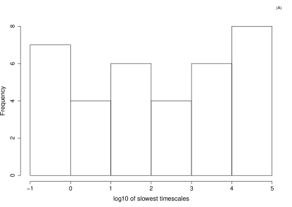
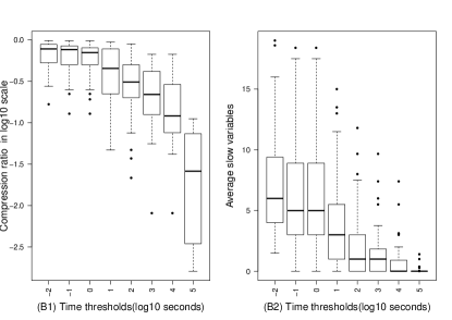
Figure 5: (A) Histogram showing the distribution of slowest timescales for $35$ models corresponding to $\varepsilon=1/23$. The quasi buffered species (cf. Sect. 4.2) are removed before performing this step. (B1) and (B2)are boxplots showing compression ratio and average number of slow variables in the Biomodels database for different values of time threshold $\theta$. The compression ratio is defined as the average number of slow variables $/$ number of variables in the model. The quasi buffered species (cf. Sect. 4.2) are removed before performing this analysis. In (B1), a point represents the compression ratio over all the tropical equilibrations for each model with respect to different time thresholds. Likewise, in (B2), a point represents the average slow variables. The number of slow variables were computed based on rescaled orders (see Eq. (17)) and certain time threshold in seconds. The time thresholds $-2$ to $5$ in the plot are the log₁₀ transformed values of time thresholds $0.01,0.1,1,10,100,1000,10000,100000$ in secs. The boxplot corresponds to $\varepsilon=1/23$. The boxplots of other $\varepsilon$ values look similar.

4.3 Tree Pruning

In order to evaluate the efficiency of tree pruning, we computed the ratio between the number of times the linear programming is invoked with some tree pruning step (cf. Fig. 2) and the possible number of combinations of Newton polytope edges without tree pruning (cf. Eq. 26). This ratio is a measure of efficiency achieved due to pruning. From the computations, it can be seen that for smaller dimensional models the logarithm of this ratio is greater than $0$ meaning tree pruning works worse by invoking linear programming more than what is required without tree pruning. However, for the majority of large dimensional models the logarithm of this ratio is less than $0$ suggesting significant reduction in the search space due to pruning. The results for $\varepsilon$ value of $1/5$ are presented in Fig. 4.

4.4 Testing the method

In order to test the method we consider the cell cycle model [43] (referenced as BIOMD00000005 by Biomodels) in more detail. This is the cell cycle model example analysed in Sect.3.4.2. Here we test the detection of slow and fast species and the accuracy of model reduction.

4.4.1 Slowness index

The detection of slow fast species is tested by comparison with a numerical method introduced in [28]. This method consists in simulating trajectories $x_{i}(t)$ for each species $i$ of the model and comparing them to the imposed trajectories $x_{i}^{*}$ calculated as solutions of quasi-steady state equations cf. Eq. (6) . Precisely, $x_{i}^{*}$ is the solution of $\sum_{j}k_{j}S_{ij}\boldsymbol{x}^{\boldsymbol{\alpha_{j}}}=0$ in which all species of indices ${l}\neq i$ are replaced by their simulated values ${x_{l}}(t)$. Like in [28] we use the slowness index $I_{i}(t)=|\log_{10}(x_{i}(t)/x_{i}^{*}(t))|$ (the base of the logarithm is purely conventional). Fast species obey quasi-steady state conditions (see Eq. (6) and Sect.2.1). Therefore, for fast species, $I_{i}$ is close to zero. For slow species, the trajectories $x_{i}(t)$ are different from $x_{i}^{*}(t)$ and the index $I_{i}$ is high. Fig. 6 shows the values of this index for all the species in the cell cycle model BIOMD00000005. In our tropical method a species is fast or slow depending how the orders $\nu_{i}=\mu_{i}-a_{i}$ compare to a timescale threshold. For $\varepsilon=1/9$, we find three tropical solutions, already discussed in Sect.3.4.2. For the solution $\boldsymbol{a}_{3}$ the species 1, 2, and 5 are fast and the species 3, 4, and 6 are slow (timescales $1\text{ min}$ or slower). This solution leads to the reduced model 1 described in Sect.3.4.2. In contrast, species 5 is slow for the two other equilibrations corresponding to the reduced model 2. The numerical method based on the slowness index classifies species 1,2, and 5 as fast and is thus compatible with the new method for the tropical solution $\boldsymbol{a}_{3}$ (Fig. 6a)). The reduced model 1 corresponding to the tropical solution $\boldsymbol{a}_{3}$ reproduces with good accuracy the limit cycle oscillations of the cell cycle model as shown in Fig. 6c).

4.4.2 Accuracy of the reduction

A quantitative estimate of reduction accuracy can be based on the $L^{2}$ norm of the difference between trajectories $\boldsymbol{x}(t)$, $\boldsymbol{x}_{red}(t)$ simulated with the full and reduced model, respectively. However, because periods are slightly changed by the reduction, the error could be defined as $err=inf_{a}\|x(t)-x_{red}(at)\|/\|x(t)\|$, where $a$ is a time scaling parameter close to $1$. For the trajectories shown in Fig. 6c), $err$ is less than $0.01$ and the optimal scaling parameter is $a=1.0002$ (the relative change of the period is $0.0002$).

The two other equilibrations lead to the reduced model 2 that is at least as accurate as the reduced model 1 (in short, in the reduced model 2, species 5 is considered slow and is not eliminated). This reduction accurately reproduces the dynamics not only on the limit cycle attractor, but also when initial data is far from this attractor. This is illustrated in Fig. 6d). We have simulated the full model and the two reduced models starting from several initial data $\boldsymbol{x}_{0i},\,i=1,\ldots,3$. The initial data of the reduced models is obtained by projection on the corresponding invariant manifolds. For example, the reduced model 1 evolves on an invariant manifold whose equations (up to small correcting terms) are given by (40) and read $x_{5}=k_{6}/(k_{4}x_{2})$, $x_{1}=k_{3}x_{2}/k_{1}$. By computing the eigenvalues of the Jacobian of system (36) we found that this invariant manifold has an attractive, stable region (all eigenvalues, except the zero ones corresponding to exact conservation laws, have negative real parts) and an unstable region (where there are eigenvalues with positive real parts). The initial data vectors $\boldsymbol{x}_{01}$ and $\boldsymbol{x}_{02}$ are close to the unstable region of the invariant manifold. Therefore, trajectories starting from these initial data first get away from the manifold and after large excursions approach the attractive part of the manifold. Reduced model 2 is able to reproduce these transients but not the reduced model 1 (Fig. 6d) because the latter is valid only on the slowest attractive invariant manifold.

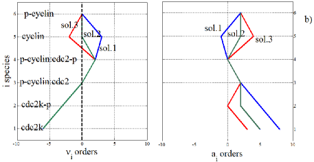
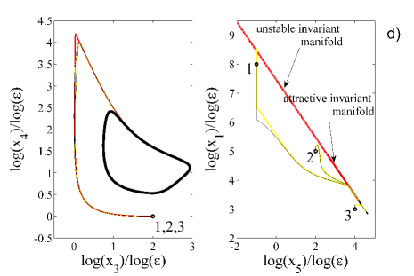
Figure 6: Testing tropical slow/fast decomposition and accuracy of reduction of BIOMD00000005 (cell cycle model). a) The slowness index is represented as a function of time on trajectories: slow variables have large slowness index (the fold ratio stands for the exponentiated index $exp(|log(x_{i}(t)/x^{*}_{i}(t))|)$); b) Left : The orders $\nu_{i}=\mu_{i}-a_{i}$ are represented for different species and for three tropical solutions. Cf. eq.(14) a species $i$ evolves on the timescale $\varepsilon^{-\nu_{i}}$ and hence lower $\nu_{i}$ mean faster species. The threshold $\theta$ separating slow and fast species set to $1\,\mathrm{min}$ to satisfy the gap condition (16) corresponds to $\mu_{\text{threshold}}=0$ as defined by (17). The threshold order is represented as a dotted line. Fast species have orders below this value, namely species $x_{1}$, $x_{2}$, $x_{5}$ are fast for the tropical solution $\boldsymbol{a}_{3}$, whereas only species $x_{1}$, $x_{2}$ are fast for the tropical solutions $\boldsymbol{a}_{1}$ and $\boldsymbol{a}_{2}$. Right : Orders $a_{i}$ for different species and tropical solutions indicate species concentrations. Cf. eq.(10) higher $a_{i}$ mean lower concentration. For all order calculations we have used $\epsilon=1/9$. c) Comparison of the limit cycle trajectories computed with the full (black circles) and reduced model (red crosses). d) Model trajectories for the full model (black), reduced model 1 (red) and reduced model 2 (yellow), starting from three initial data, corresponding to three different tropical equilibrations. The limit cycle attractor is contained in an invariant manifold. The reduced model 1 provides a good approximation of the dynamics on the invariant manifold (such as starting from initial data 3), but not outside. The reduced model 2 is accurate also outside the invariant manifold (see trajectories starting from equilibrations 1 and 2).

4.5 Comparison with COPASI time separation method

We compared our proposed method against the existing tool COPASI [16, 41]. COPASI is a software for simulation and analysis of biochemical networks. This software accepts and generates several model exchange formats including the widely spread systems biology markup language (SBML) format and is very popular in the computational biology community. To the best of our knowledge, COPASI is the only major biochemical networks tool that implements time separation of variables. To accomplish this aim COPASI proposes a modified ILDM (intrinsic low dimensional manifold) method. This method computes slow and fast modes which are transformations of species concentrations as described in [4, 46, 41]. More precisely, COPASI performs a Schur block decomposition of the Jacobian matrix $\boldsymbol{J}$, consisting in finding a non-singular matrix $T$ such that $T^{-1}JT=\begin{pmatrix}S_{slow}&0\\ 0&S_{fast}\end{pmatrix}$, where $S_{slow},S_{fast}$ have real Schur form, i.e. they are upper triangular matrices with possibly non-vanishing elements on the first subdiagonal. The time threshold (needed to separate the slow and fast blocks of the Jacobian matrix) is automatically captured in this method by finding a gap in the spectrum of the Jacobian (cf. Sect.2.1).

In order to compare the modified ILDM method against our tropical and slowness index methods, we computed the fast space of the model using COPASI for $100$ time steps between $1$ and $100$ min and checked the contribution of each species to this fast space. COPASI defines the contribution of a species $i$ to a mode $j$ as the matrix element $T^{-1}_{ji}$. These contributions of various species to fast modes are provided by COPASI as fractions $p_{i}$, where $i$ is the species index, $0\leq p_{i}\leq 1,\,\sum_{i}p_{i}=1$. COPASI declare species with largest contribution to the fast space (largest $p_{i}$) as fast species. For exactly the same trajectory, we have computed the values of the slowness indices ${I}_{i}=|\log_{10}(x_{i}(t)/x^{*}_{i}(t))|$. For fast species, $I_{i}$ should be close to zero. Fig. 6a) and b) summarizes the comparison between the slowness index and the tropical method. The tropical solution $\boldsymbol{a}_{3}$ leads to the reduced model 1 (cf. Sect.3.4.2) and copes with the limit cycle trajectory used in this test. The timescale orders $\nu_{i}$ of the variables for this tropical solutions identify species $x_{1}$, $x_{2}$, $x_{5}$ as fast and species $x_{3}$, $x_{4}$, $x_{6}$ as slow (see also Sect.3.4.2). As can been seen in Fig. 6a) the slowness index of species $x_{1}$, $x_{2}$, $x_{5}$ is close to zero for all times. The slowness index of species $x_{3}$, $x_{4}$, $x_{6}$ can reach large values. Therefore the tropical method and the slowness index method provide exactly the same timescale decomposition. COPASI time separation can not be compared directly to the tropical method, because it generates a timescale decomposition that changes with time and which is valid for a trajectory. However, it can be compared with the slowness index decomposition. Fig. 7 summarizes the comparison between COPASI and the slowness index. It should be noted that the species $x_{3}$ is automatically eliminated by COPASI using the single conservation law present in the model. The slowness index and COPASI contribution to fast space should be anticorrelated: when the first one is small the latter should be big and vice versa. Species $x_{1}$ and $x_{5}$ have high contribution towards the fast space and very low slowness index (see Fig. 7b). For these species we can say there is consistence between COPASI and slowness index. Species $x_{2}$ also has large contribution to fast space except for some intervals where COPASI may classify it as slow. Our method unambiguously classifies this species as fast (cf. Fig. 7b) its slowness index is very low for all times). Most importantly, COPASI fails to identify correctly time intervals where species $6$ is slow as indicated by the large value of the slowness index co-existing with large values of contribution $p_{i}$ (as large as for species $1$ and $2$, see Fig. 7b). According to COPASI this species is similar to the fast species $x_{2}$, whereas our methods indicate it is similar to the slow species $x_{4}$ and $x_{3}$. As a matter of fact, COPASI determines slow variables by comparing the values of contributions $p_{i}$ to the fast and slow modes. Despite the existence of a spectral gap, the differences of the indices $p_{i}$ between species that are considered slow and fast can be relatively small and therefore this classification is not robust. In contrast, our methods classify species in a robust way. Indeed, we directly associate timescales to species, via the orders $\nu_{i}$ and these timescales are well separated for slow and fast species. Using these orders, we found that the fastest slow species $x_{3}$ and $x_{6}$ are $100$ times slower than the slower fast species $x_{5}$. Furthermore, as shown in Fig.6a, our slowness index is very sensitive to differences in timescales. Fast species $x_{1}$, $x_{2}$, $x_{5}$ keep this index low for all times, whereas the corresponding COPASI indices are not always high. Generally, it should not be recommended to use species contributions to modes as indicative of their timescales, as COPASI does. For instance, the sum of two or more species can be a slow mode, even if all these species are fast (cf. Sect. 2.3, this situation is typical for fast cycles). The fast species have in this case high contributions to a slow mode which may qualify them as slow according to the species contribution criterion.

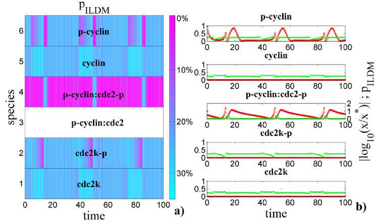
Figure 7: Summary of the analysis of model BIOMD00000005 using ILDM method and comparison with our method based on the slowness index. The model was simulated in COPASI from $0$ to $100$ min with default initial concentrations. The species $3$ is eliminated using the single conservation law. For all the remaining species we represent the time dependence of their contributions $p_{i}$, where $0\leq p_{i}\leq 1,\,\sum_{i}p_{i}=1$ to the fast space. The fractions $p_{i}$ are generated by COPASI and the values $p_{i}$ are color coded in the left panel a). Chemical species with largest contribution to the fast space (largest $p_{i}$) are supposed to be fast species (as explained in [41]). Therefore $p_{i}$ (in green in right panel b)) and our slowness index $I_{i}=|\log_{10}(x_{i}/x_{i}^{*})|$ (in red) should be anti-correlated. This is well verified for species $1,4,5$ ($p_{i}$ are relatively high when $I_{i}$ are close to zero, and close to zero when $I_{i}$ are relatively high, but it is not well verified for species $6$ (p-cyclin) whose slowness index has large peaks in places where the COPASI contribution to fast modes stays constantly high.

5 Conclusion

We have addressed the problems of timescale decomposition and model reduction of biochemical networks. Our approach relies on the notion of tropical equilibration. Tropical equilibrations represent a generalization of steady states and correspond to compensation of dominant fluxes acting on species concentrations. The remaining, uncompensated weaker fluxes are responsible for the slow dynamics of the system on attractive invariant manifolds. The correspondence between tropical equilibrations and attractive invariant manifolds has been exploited here to associate, to each tropical equilibration, a reduced model. We show elsewhere [33] that when there is an infinity of tropical equilibration solutions, these can be organised into branches, each branch corresponding to the same reduced model.

We have proposed an algorithm to compute tropical equilibrations. We have used this algorithm to determine the fast/slow partition of chemical species in a network of biochemical reactions that is the first and often critical step in model reduction algorithms. In particular, the number of slow species provides the size of minimal dynamic models to which complex biochemical networks can be reduced. The validity of our reductions depends on concentration and parameter orders, as well as on initial data. For the simple example of Michaelis-Menten kinetics we obtained validity conditions for various reductions as inequalities among orders of magnitude of concentrations and parameters. These validity conditions define large domains in the concentrations and parameters spaces. Previous work on larger models suggests a larger applicability of this result which implies that the resulting reductions are robust [28].

The benchmarking of our algorithm on the Biomodels database shows that a significant dimension compression can be performed on cell dynamics models at timescales of $1000s$ and larger. Starting with complex models having more than 30 variables, minimal models have median numbers of 2 slow variables. This suggests that, at least piece-wise in parameter and phase space, the tasks fulfilled by molecular networks are relatively simple. The need for having complex machineries with many regulators to perform simple tasks (such as relaxation to steady states or limit cycle oscillations) could be justified by system robustness. A system having a very large number of variables and parameters, multiple timescales and only a few slow degrees of freedom is generically robust with respect to perturbations of variables and parameters [10].

Our methods can be also used to study sensitivity issues and identifiability of parameters from trajectories. A parameter is sensitive if changing its value induces large changes of model trajectories. In our analysis of Tyson’s model we have seen that some parameters of the full model are not present in the reduced model. Although the orders of magnitude of these parameters are important (changing them may change the reduction), small changes of their values do not lead to changes of the model trajectories. Parameters of the full model that are not present in the reduced model are therefore insensitive. It may also happen that parameters of the reduced model are combinations (for instance multivariate monomials) of the parameters of the full model. If these combinations are sensitive, then so are the parameters they contain. However, parameters that are parts of such combinations can not be determined independently from the observed trajectories, which leads to parameter non-identifiability issues [29]. Thus, insensitive parameters and parameter lumping resulting from model reduction can be used to asses local identifiability of system parameters [29]. The idea of relating parameter lumping and parameter identifiability can also be found in other computational algebraic geometry approaches [23].

Solving the tropical equilibration problem and finding a slow-fast decomposition is the first step for model reduction. The remaining steps consist in elimination of the fast variables by solving systems of algebraic equations. We have shown how this can be performed for simple examples. In the case of more complex models, the elimination can be performed numerically, or symbolically. Tropical methods can simplify this task by replacing the full systems by tropically truncated systems. In particular, the binomial or toric case when the truncation has only two monomials is particularly interesting because for this case there are rapid algorithms for computing steady states [24]. Higher approximation can be provided by Newton-Puiseux expansions [30], that encompass tropical solutions in their lowest order. Although the calculations needed for formal reduction could be long, once the model is reduced, it can be used in various applications, such as a part of larger networks, or in models of tissues and organisms where the same biochemical network has to be replicated in several interacting cells. Furthermore, our reductions have a strong geometrical basis. In future work, we will exploit this property to show how to endow the reduced model with a reaction network structure and how to identify inclusion relations among different reduced models.

Several other open questions will be addressed in future work. For instance, our current algorithm finds the tropical equilibrations for fixed values of the parameters. It would be very interesting to formally classify all the possible reductions and phase portraits of a reaction network with a given topology and reaction rates, for all possible values of the parameters. We have solved this problem by hand for the Michaelis-Menten kinetics. In the future we will extend our algorithms in order to compute how the tropical equilibration solutions depend on parameters. For this purpose we will extend techniques used for linear quantifier elimination [45, 5, 44] and incorporate them into Algorithm 1.

Acknowledgements.

This work has been supported by the French ModRedBio CNRS Peps, and EPIGENMED Excellence Laboratory projects. D.G. is grateful to the Max-Planck Institut für Mathematik, Bonn for its hospitality during writing this paper and to Labex CEMPI (ANR-11-LABX-0007-01).

References

- [1] Chang, C.S.: On deterministic traffic regulation and service guarantees: a systematic approach by filtering. IEEE Transactions on Information Theory 44(3), 1097–1110 (1998)
- [2] Chiavazzo, E., Karlin, I.: Adaptive simplification of complex multiscale systems. Physical Review E 83(3), 036,706 (2011)
- [3] Clarke, E.M., Grumberg, O., Peled, D.: Model checking. MIT press (1999)
- [4] Deuflhard, P., Heroth, J.: Dynamic dimension reduction in ODE models. Springer (1996)
- [5] Dolzmann, A., Sturm, T.: REDLOG: Computer algebra meets computer logic. ACM SIGSAM Bulletin 31(2), 2–9 (1997)
- [6] Feret, J., Danos, V., Krivine, J., Harmer, R., Fontana, W.: Internal coarse-graining of molecular systems. Proceedings of the National Academy of Sciences 106(16), 6453–6458 (2009). DOI 10.1073/pnas.0809908106. URL http://www.pnas.org/content/106/16/6453.abstract
- [7] Gawrilow, E., Joswig, M.: Polymake: a framework for analyzing convex polytopes. Polytopes Combinatorics and Computation (2000). URL http://link.springer.com/chapter/10.1007/978-3-0348-8438-9_2
- [8] Gorban, A., Karlin, I.: Invariant manifolds for physical and chemical kinetics, Lect. Notes Phys. 660. Springer, Berlin, Heidelberg (2005)
- [9] Gorban, A., Radulescu, O.: Dynamic and static limitation in reaction networks, revisited . In: D.W. Guy B. Marin, G.S. Yablonsky (eds.) Advances in Chemical Engineering - Mathematics in Chemical Kinetics and Engineering, Advances in Chemical Engineering, vol. 34, pp. 103–173. Elsevier (2008). DOI 10.1016/S0065-2377(08)00002-1
- [10] Gorban, A.N., Radulescu, O.: Dynamical robustness of biological networks with hierarchical distribution of time scales. IET Systems Biology 1(4), 238–246 (2007)
- [11] Gorban, A.N., Radulescu, O., Zinovyev, A.Y.: Asymptotology of chemical reaction networks. Chemical Engineering Science 65(7), 2310–2324 (2010). DOI 10.1016/j.ces.2009.09.005. International Symposium on Mathematics in Chemical Kinetics and Engineering
- [12] Gorban, A.N., Shahzad, M.: The Michaelis-Menten-Stueckelberg theorem. Entropy 13(5), 966–1019 (2011)
- [13] Gurobi Optimization: Gurobi optimizer reference manual (2012). URL URL: http://www.gurobi.com
- [14] Haller, G., Sapsis, T.: Localized instability and attraction along invariant manifolds. SIAM Journal on Applied Dynamical Systems 9(2), 611–633 (2010)
- [15] Henk, M., Richter-Gebert, J., Ziegler, G.M.: 16 basic properties of convex polytopes. Handbook of discrete and computational geometry p. 355 (2004)
- [16] Hoops, S., Sahle, S., Gauges, R., Lee, C., Pahle, J., Simus, N., Singhal, M., Xu, L., Mendes, P., Kummer, U.: COPASI – a complex pathway simulator. Bioinformatics 22(24), 3067–3074 (2006). DOI 10.1093/bioinformatics/btl485. URL http://bioinformatics.oxfordjournals.org/content/22/24/3067.abstract
- [17] Lam, S., Goussis, D.: The CSP method for simplifying kinetics. International Journal of Chemical Kinetics 26(4), 461–486 (1994)
- [18] Le Novere, N., Bornstein, B., Broicher, A., Courtot, M., Donizelli, M., Dharuri, H., Li, L., Sauro, H., Schilstra, M., Shapiro, B., Snoep, J.L., Hucka, M.: BioModels database: a free, centralized database of curated, published, quantitative kinetic models of biochemical and cellular systems. Nucleic Acids Research 34(suppl 1), D689–D691 (2006). DOI 10.1093/nar/gkj092. URL http://nar.oxfordjournals.org/content/34/suppl_1/D689.abstract
- [19] Litvinov, G.: Maslov dequantization, idempotent and tropical mathematics: a brief introduction. Journal of Mathematical Sciences 140(3), 426–444 (2007)
- [20] Maas, U., Pope, S.B.: Simplifying chemical kinetics: intrinsic low-dimensional manifolds in composition space. Combustion and Flame 88(3), 239–264 (1992)
- [21] Maclagan, D., Sturmfels, B.: Introduction to tropical geometry. American Mathematical Society, RI (2015)
- [22] Meiske, W.: An approximate solution of the michaelis-menten mechanism for quasi-steady and state quasi-equilibrium. Mathematical Biosciences 42(1), 63–71 (1978)
- [23] Meshkat, N., Eisenberg, M., DiStefano, J.J.: An algorithm for finding globally identifiable parameter combinations of nonlinear ode models using Gröbner bases. Mathematical biosciences 222(2), 61–72 (2009)
- [24] Millán, M.P., Dickenstein, A., Shiu, A., Conradi, C.: Chemical reaction systems with toric steady states. Bulletin of mathematical biology 74(5), 1027–1065 (2012)
- [25] Noel, V., Grigoriev, D., Vakulenko, S., Radulescu, O.: Tropical geometries and dynamics of biochemical networks application to hybrid cell cycle models. In: J. Feret, A. Levchenko (eds.) Proceedings of the 2nd International Workshop on Static Analysis and Systems Biology (SASB 2011), Electronic Notes in Theoretical Computer Science, vol. 284, pp. 75–91. Elsevier (2012)
- [26] Noel, V., Grigoriev, D., Vakulenko, S., Radulescu, O.: Tropical and Idempotent Mathematics and Applications, vol. 616, chap. Tropicalization and tropical equilibration of chemical reactions. American Mathematical Society (2014)
- [27] Pachter, L., Sturmfels, B.: Tropical geometry of statistical models. Proceedings of the National Academy of Sciences of the United States of America 101(46), 16,132 (2004)
- [28] Radulescu, O., Gorban, A.N., Zinovyev, A., Lilienbaum, A.: Robust simplifications of multiscale biochemical networks. BMC systems biology 2(1), 86 (2008)
- [29] Radulescu, O., Gorban, A.N., Zinovyev, A., Noel, V.: Reduction of dynamical biochemical reactions networks in computational biology. Frontiers in Genetics 3(131) (2012). DOI 10.3389/fgene.2012.00131
- [30] Radulescu, O., Vakulenko, S., Grigoriev, D.: Model reduction of biochemical reactions networks by tropical analysis methods. Mathematical Model of Natural Phenomena 10(3), 124–138 (2015)
- [31] Rowley, C.W., Marsden, J.E.: Reconstruction equations and the Karhunen–Loève expansion for systems with symmetry. Physica D: Nonlinear Phenomena 142(1), 1–19 (2000)
- [32] Samal, S.S., Errami, H., Weber, A.: PoCaB: a software infrastructure to explore algebraic methods for bio-chemical reaction networks. In: V.P. Gerdt, W. Koepf, E.W. Mayr, E.V. Vorozhtsov (eds.) Computer Algebra in Scientific Computing, Lecture Notes in Computer Science, vol. 7442, pp. 294–307. Springer Berlin Heidelberg (2012). DOI 10.1007/978-3-642-32973-9_25. URL http://dx.doi.org/10.1007/978-3-642-32973-9_25
- [33] Samal, S.S., Grigoriev, D., Fröhlich, H., Radulescu, O.: Analysis of reaction network systems using tropical geometry. In: V.P. Gerdt, W. Koepf, W.M. Seiler, E.V. Vorozhtsov (eds.) Computer Algebra in Scientific Computing – 17th International Workshop (CASC 2015), Lecture Notes in Computer Science, vol. 9301, pp. 422–437. Springer, Aachen, Germany (2015). DOI 10.1007/978-3-319-24021-3_31
- [34] Savageau, M., Voit, E.: Recasting nonlinear differential equations as S-systems: a canonical nonlinear form. Mathematical biosciences 87(1), 83–115 (1987)
- [35] Savageau, M.A., Coelho, P.M., Fasani, R.A., Tolla, D.A., Salvador, A.: Phenotypes and tolerances in the design space of biochemical systems. Proceedings of the National Academy of Sciences 106(16), 6435–6440 (2009)
- [36] Segel, L.A.: On the validity of the steady state assumption of enzyme kinetics. Bulletin of mathematical biology 50(6), 579–593 (1988)
- [37] Segel, L.A., Slemrod, M.: The quasi-steady-state assumption: a case study in perturbation. SIAM review 31(3), 446–477 (1989)
- [38] Simon, I.: Recognizable sets with multiplicities in the tropical semiring. In: Mathematical Foundations of Computer Science 1988, pp. 107–120. Springer (1988)
- [39] Soliman, S., Fages, F., Radulescu, O.: A constraint solving approach to model reduction by tropical equilibration. Algorithms for Molecular Biology 9(1), 24 (2014)
- [40] Sturmfels, B.: Solving systems of polynomial equations. CBMS Regional Conference Series in Math., no. 97, American Mathematical Society, Providence, RI (2002)
- [41] Surovtsova, I., Simus, N., Lorenz, T., König, A., Sahle, S., Kummer, U.: Accessible methods for the dynamic time-scale decomposition of biochemical systems. Bioinformatics 25(21), 2816–2823 (2009). DOI 10.1093/bioinformatics/btp451. URL http://bioinformatics.oxfordjournals.org/content/25/21/2816.abstract
- [42] Tikhonov, A.N.: Systems of differential equations containing small parameters in the derivatives. Matematicheskii sbornik 73(3), 575–586 (1952)
- [43] Tyson, J.J.: Modeling the cell division cycle: cdc2 and cyclin interactions. Proceedings of the National Academy of Sciences 88(16), 7328–7332 (1991)
- [44] Weber, A., Sturm, T., Abdel-Rahman, E.O.: Algorithmic global criteria for excluding oscillations. Bulletin of Mathematical Biology 73(4), 899–916 (2011). DOI 10.1007/s11538-010-9618-0. URL http://dx.doi.org/10.1007/s11538-010-9618-0
- [45] Weispfenning, V.: The complexity of linear problems in fields. Journal of Symbolic Computation 5(1&2), 3–27 (1988)
- [46] Zobeley, J., Lebiedz, D., Kammerer, J., Ishmurzin, A., Kummer, U.: A new time-dependent complexity reduction method for biochemical systems. In: Transactions on Computational Systems Biology I, pp. 90–110. Springer (2005)