Shape Complexes in Continuous Max-Flow Hierarchical Multi-Labeling Problems

Abstract

Although topological considerations amongst multiple labels have been previously investigated in the context of continuous max-flow image segmentation, similar investigations have yet to be made about shape considerations in a general and extendable manner. This paper presents shape complexes for segmentation, which capture more complex shapes by combining multiple labels and super-labels constrained by geodesic star convexity. Shape complexes combine geodesic star convexity constraints with hierarchical label organization, which together allow for more complex shapes to be represented. This framework avoids the use of co-ordinate system warping techniques to convert shape constraints into topological constraints, which may be ambiguous or ill-defined for certain segmentation problems.

1 INTRODUCTION

Since the proliferation of graph-cuts as an image segmentation mechanism[1], there has been a great amount of interest in expanding the methods to address problems in which more global information about the segmented objects is known. Topological considerations in terms of label orderings have allowed objects to be broken into and reassembled from distinct constituents, resulting in linear (or Ishikawa) models[2], submodular graph models[3], and hierarchical models[4]. Global knowledge about the geometry of individual labels have led to approaches such as graph-cut-based shape templates[5] and graph-cut-accelerated statistical shape models[6].

Shape information that can be implemented within a single graph-cut are particularly interesting in that they maintain submodularity and therefore guarantee global optimality. Often, these are formulated as constraints on the segmentation itself via additional infinite-cost edges between nodes. Simple star convexity[7] and geodesic star convexity[8] in particular use infinite-cost edges to constrain objects to be connected to a predefined vantage point through either a straight path (for simple star convexity) or a geodesic (for geodesic star convexity).

For both label ordering considerations and shape information, continuous counterparts to discrete graph cuts have been developed. In terms of label ordering, Bae et al.[9] extended the Ishikawa model. Baxter et al.[10, 11] extended the hierarchical model and developed a framework for arbitrary label orderings. For simple and geodesic star convexity, Yuan et al.[12] and Ukwatta el al.[13] provided two alternative solutions in the continuous domain. However, there has yet to be an general-purpose, extendable framework that combines topological and shape considerations simultaneously.

2 Contributions

The contribution of this paper is the definition of shape complexes. Shape complexes are a collection of partially ordered labels in which several are constrained to have geodesic star convexity, thus addressing topological and shape considerations simultaneously. The result is that many additional shape constraints (such as rings) can be represented on multiple distinct objects simultaneously while maintaining a single co-ordinate system.

3 Previous Work

Yuan et al.[12] developed the first geodesic star convexity constraint in continuous max-flow segmentation, addressing optimization problems of the form:

$$\underset{u}{\min} E(u)=\sum\limits_{\forall L}\int_{\Omega}\left(D(x)u(x)+S(x)|\nabla u(x)|\right)dx$$ (1)

subject to $$u(x)\in\{0,1\}\text{ and }\nabla u(x)\cdot e(x)\geq 0$$

where $u(x)$ is the labeling function and $e(x)$ is the local direction of the geodesic. This was addressed through the use of convex relaxation and primal-dual optimization using the labeling $u(x)$ and $1-u(x)$, as well as one additional field $\lambda(x)$ as multipliers. $\lambda(x)$ was used to ensure that the inequality constraint $\nabla u(x)\cdot e(x)\geq 0$ was respected, ensuring geodesic star convexity.

A very different approach was taken by Ukwatta et al.[13] in order to implement geodesic star convexity. In his approach, the image co-ordinate system is warped, each in-plane image cross-section being represented in cylindrical co-ordinates with the center point placed somewhere in the object of interest, i.e. the interior blood pool of the femoral arterial. When expressed as such, simple star convexity can be expressed as a topological constraint, that is, as a continuous Ishikawa[9] model. This has the additional benefit that multiple simple star convexity constraints can be placed. In the framework proposed by Ukwatta et al.[13], both the vessel interior and the entire vessel (the union of the interior and wall labels) are constrained to have simple star convexity. Geodesic star convexity could be implemented by furthering warping of this co-ordinate system transformation.

However, these resampling approaches can be subject to ambiguity and ill-definition in a variety of cases. For the sake of example, consider vascular segmentation in which the vessel being segmentation bifurcates. After that bifurcation, no single center point can be defined, thus rendering the co-ordinate transformation ill-defined. The transformation may be ambiguous when the vascular ‘bends back’ on itself creating a U shape, causing multiple slices to intersect after warping. Illustrative versions of these three cases (including the non-ambiguous, well-defined case) are shown in Figure 1.

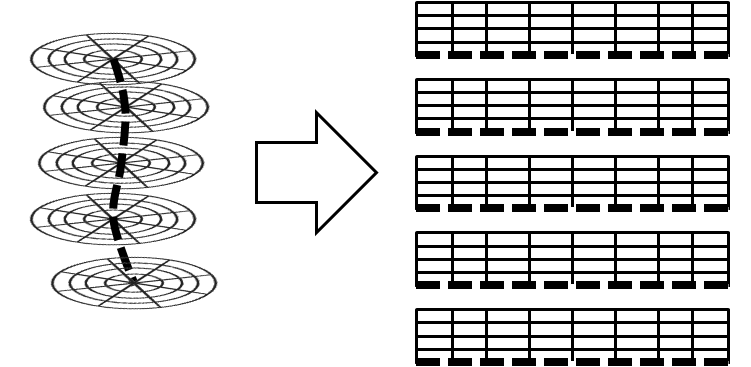
(a) Case in which cylindrical warping is neither ill-defined nor ambiguous.

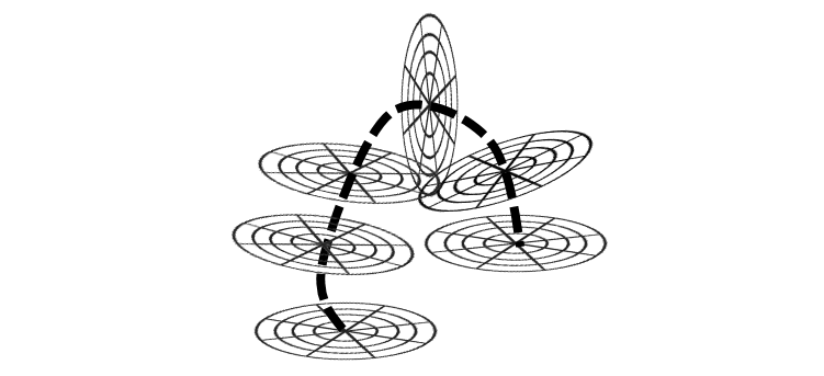
(b) Case in which cylindrical warping is ambiguous due to locations that are represented multiple times in the new warped co-ordinate system.

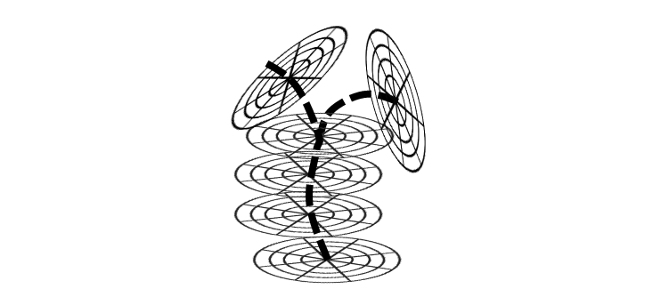
(c) Case in which cylindrical warping is ill-defined as no single curve can represent both distinct sets of center points (bifurcation).

Figure 1: Three possible cases for co-ordinate system warping

Ultimately, the issues associated with co-ordinate system warping become more intractable as the number of distinct labels with geodesic star convexity increases, resulting in more ill-definition or warping ambiguity, as multiple interacting co-ordinate systems must be defined.

4 Shape Complexes in Continuous Max-Flow Segmentation

4.1 Continuous Max-Flow Model

This paper extends the work of Baxter et al.[10] on generalized hierarchical continuous max-flow (GHMF) models. Baxter et al. used the method of primal-dual optimization with augmented Lagrangian multipliers to address a max-flow min-cut problem through a directed tree of continuous spaces. The directed tree or hierarchy encodes the label ordering in the form of super-labels partitioned into their constituent parts with leaf nodes representing the ultimate partition of the whole image. The minimization equation we intend to solve extends the GHMF minimization equation:

$$\underset{u}{\min} E(u)=\sum\limits_{\forall L}\int_{\Omega}\left(D_{L}(x)u_{L}(x)+S_{L}(x)|\nabla u_{L}(x)|\right)dx$$ (2)

subject to $$\forall L(u_{L}(x)\geq 0)$$

$$\forall L\left(\sum\limits_{L^{\prime}\in L.C}u_{L^{\prime}}(x)=u_{L}(x)\right)$$

$$u_{S}(x)=1$$

by the addition of the constraint originally posed by Yuan et al.[12]:

$$\nabla u_{L}(x)\cdot e_{L}(x)\geq 0$$

This constraint dictates that for each label at each pixel, there is a direction $e_{L}(x)$ in which assigning the label $L$ to voxel $x$ entails giving the same label to voxels proximal to $x$ in the positive $e_{L}(x)$ direction. If all of these direction vectors point at a single spatial location, this enforces simple star convexity. If this direction field is warped, it enforces geodesic star convexity.

The approach taken will be analogous to the augmented Lagrangian approach taken by Yuan et al.[14, 12].

4.2 Primal Formulation

As in the previous work, the primal formulation will be expressed as a max-flow optimization, specifically:

$$\underset{p,q^{\prime},\lambda}{\max} \int_{\Omega}p_{S}(x)dx$$ (3)

subject to the capacity constraints:

$$p_{L}(x) \leq D_{L}(x),\text{ }L\in\text{ leaves}$$

$$|q^{\prime}_{L}(x)| \leq S_{L}(x)\text{ }L\neq S$$

$$\lambda_{L}(x) \geq 0$$

and the flow conservation constraint:

$$0=\operatorname{div}\left(q^{\prime}_{L}(x)+\lambda_{L}(x)e_{L}(x)\right)+p_{L}(x)-p_{L.P}(x)\text{ .}$$

$q^{\prime}_{L}(x)$, the spatial flow not including flow along the infinite capacity direction $e_{L}(x)$, is distinguished from $q_{L}(x)$, the overall spatial flow, noting that $q_{L}(x)=q^{\prime}_{L}(x)+\lambda_{L}(x)e_{L}(x)$. Here we depart from the approach taken by Yuan et al.[12] by rewriting Eq. (3) in terms of $q_{L}(x)$ instead of $q^{\prime}_{L}(x)$ yielding the formula:

$$\underset{p,q,\lambda}{\max} \int_{\Omega}p_{S}(x)dx$$

subject to the constraints:

$$p_{L}(x) \leq D_{L}(x),\text{ }L\in\text{ leaves}$$

$$|q_{L}(x)-\lambda_{L}(x)e_{L}(x)| \leq S_{L}(x)\text{ }L\neq S$$

$$\lambda_{L}(x) \geq 0$$

$$0 =\operatorname{div}q_{L}(x)+p_{L}(x)-p_{L.P}(x)$$

in which it should be noted that $\lambda$ can be explicitly solved for, appearing only in the constraints $\lambda(x)\geq 0$ and $|q_{L}(x)-\lambda_{L}(x)e_{L}(x)|\leq S_{L}(x)$. In order to ensure the spatial capacity constraint, the value of $|q_{L}(x)-\lambda_{L}(x)e_{L}(x)|$ should be minimized over $\lambda_{L}(x)\geq 0$. This can be done analytically by finding the projection of $q_{L}(x)$ onto $e_{L}(x)$, ignoring any component of $q_{L}(x)$ in the $-e_{L}(x)$ direction. Thus, $\lambda_{L}(x)=\max\{0,q_{L}(x)\cdot e_{L}(x)\}$ assuming without loss of generality that $e_{L}(x)$ is unit length if a geodesic direction is specified and zero length if not. The final primal formulation is:

$$\underset{p,q}{\max} \int_{\Omega}p_{S}(x)dx$$ (4)

subject to the constraints:

$$p_{L}(x) \leq D_{L}(x),\text{ }L\in\text{ leaves}$$

$$|q_{L}(x)-\lambda(x)e_{L}(x)| \leq S_{L}(x)\text{ }L\neq S\text{ where }\lambda_{L}(x)=\max\{0,q_{L}(x)\cdot e_{L}(x)\}$$

$$0 =\operatorname{div}q_{L}(x)+p_{L}(x)-p_{L.P}(x)$$

4.3 Primal-Dual Formulation

In order to develop the primal-dual formulation, we use the method of Lagrangian multipliers over the primal equation (4) on the flow conservation constraint $G_{L}(x)=\operatorname{div}q_{L}(x)+p_{L}(x)-p_{L.P}(x)=0$, yielding the equation:

$$\underset{u}{\min}\underset{p,q}{\max} \left(\int_{\Omega}p_{S}(x)dx+\sum_{\forall L\neq S}\int_{\Omega}u_{L}(x)G_{L}(x)dx\right)$$ (5)

$$p_{L}(x) \leq D_{L}(x),\text{ }L\in\text{ leaves}$$

$$|q_{L}(x)-\lambda(x)e_{L}(x)| \leq S_{L}(x)\text{ }L\neq S\text{ where }\lambda_{L}(x)=\max\{0,q_{L}(x)\cdot e_{L}(x)\}\text{ .}$$

To ensure that this equation is optimizable, meeting the requirements of the minimax theorem, we must ensure that it is convex with respect to $u$, considering $p,q$ to be fixed, and concave with respect to $p,q$ with $u$ fixed.[15] Holding $p$ and $q$ fixed, $G$ is also fixed and thus Eq. (5) is linear with no constraints and is therefore concave. If $u$ is fixed, Eq. (5) is linear with convex constraints and is therefore convex. Thus Eq. (5) can be optimized.

4.4 Dual Formulation

To show the equivalence of Eqs. (2) and (5), we will consider the optimization of each set of flows in a bottom-up manner similar to GHMF[10]. Starting with any leaf node in the tree we can isolate $p_{L}$ in (5) as:

$$\underset{u}{\min}\underset{p_{L}(x)\leq D_{L}(x)}{\max}\int_{\Omega}u_{L}(x)p_{L}(x)dx=\underset{u,u_{L}(x)\geq 0}{\min}\int_{\Omega}u_{L}(x)D_{L}(x)dx$$ (6)

(If $u_{L}(x)<0$, the function can be arbitrarily maximized by $p_{L}(x)\to-\infty$.) Every branch label can then be isolated as:

$$\underset{u}{\min}\underset{p_{L}(x)}{\max}\left(\int_{\Omega}u_{L}(x)p_{L}(x)dx-\sum_{\forall L^{\prime}\in L.C}\int_{\Omega}u_{L^{\prime}}(x)p_{L}(x)dx\right)=0$$ (7)

at the saddle point defined by $u_{L}(x)=\sum_{\forall L^{\prime}\in L.C}u_{L^{\prime}}(x)$. The source flow, $p_{S}$, can be isolated similarly as:

$$\underset{u}{\min}\underset{p_{S}(x)}{\max}\left(\int_{\Omega}p_{S}(x)dx-\sum_{\forall L^{\prime}\in S.C}\int_{\Omega}u_{L^{\prime}}(x)p_{S}(x)dx\right)=0$$ (8)

at the saddle point defined by $1=\sum_{\forall L^{\prime}\in S.C}u_{L^{\prime}}(x)$. These constraints combined yield the labeling constraints in the original formulation.

To maximize the spatial flows, we will use the first primal formulation Eq. (3) and separate the spatial flows into $q^{\prime}_{L}(x)$ and $\lambda_{L}(x)e_{L}(x)$. Considering $q^{\prime}_{L}(x)$ first, the maximization can be expressed as described by Giusti [16]] as:

$$\int_{\Omega}u_{L}(x)\operatorname*{\operatorname{div}}q^{\prime}_{L}(x)dx =\int_{\Omega}\left(\operatorname*{\operatorname{div}}(u_{L}(x)q^{\prime}_{L}(x))-q^{\prime}(x)\cdot\nabla u_{L}(x)\right)dx$$ (9)

$$=\int_{\Omega}\operatorname*{\operatorname{div}}(u_{L}(x)q^{\prime}_{L}(x))dx-\int_{\Omega}q^{\prime}_{L}(x)\cdot\nabla u_{L}(x)dx$$

$$=\oint_{\delta\Omega}u_{L}(x)q^{\prime}_{L}(x)\cdot d\mathbf{s}-\int_{\Omega}q^{\prime}_{L}(x)\cdot\nabla u_{L}(x)dx$$

$$=-\int_{\Omega}q^{\prime}_{L}(x)\cdot\nabla u_{L}(x)dx$$

$$\underset{|q^{\prime}_{L}|\leq S_{L}(x)}{\max}\int_{\Omega}u_{L}(x)\operatorname*{\operatorname{div}}q^{\prime}_{L}(x)dx =\underset{|q^{\prime}_{L}|\leq S_{L}(x)}{\max}-\int_{\Omega}q^{\prime}_{L}(x)\cdot\nabla u_{L}(x)dx$$

$$=-\int_{\Omega}\left(-\frac{S_{L}(x)}{|\nabla u_{L}(x)|}\nabla u_{L}(x)\right)\cdot\nabla u_{L}(x)dx$$

$$=\int_{\Omega}S_{L}(x)|\nabla u_{L}(x)|dx$$

$$\underset{u_{L}\geq 0}{\min}\;\;\underset{|q^{\prime}_{L}|\leq S_{L}(x)}{\max}\int_{\Omega}u_{L}(x)\operatorname*{\operatorname{div}}q_{L}(x)dx =\underset{u_{L}\geq 0}{\min}\int_{\Omega}S_{L}(x)|\nabla u_{L}(x)|dx\text{ .}$$

Taking the same approach to $\lambda_{L}(x)e_{L}(x)$:

$$\int_{\Omega}u_{L}(x)\operatorname*{\operatorname{div}}\left(\lambda_{L}(x)e_{L}(x)\right)dx =\int_{\Omega}u_{L}(x)\left(\nabla\lambda(x)\cdot e_{L}(x)\right)dx+\int_{\Omega}u_{L}(x)\lambda(x)\operatorname*{\operatorname{div}}e_{L}(x)dx$$ (10)

$$=\int_{\Omega}\nabla\lambda(x)\cdot u_{L}(x)e_{L}(x)dx+\int_{\Omega}\lambda(x)\operatorname*{\operatorname{div}}\left(u_{L}(x)e_{L}(x)\right)dx-\int_{\Omega}\lambda(x)\left(\nabla u_{L}(x)\cdot e_{L}(x)\right)$$

$$=\int_{\Omega}\operatorname*{\operatorname{div}}\left(\lambda(x)u_{L}(x)e_{L}(x)\right)dx-\int_{\Omega}\lambda(x)\left(\nabla u_{L}(x)\cdot e_{L}(x)\right)$$

$$=\oint_{\delta\Omega}\lambda(x)u_{L}(x)e_{L}(x)\cdot d\mathbf{s}-\int_{\Omega}\lambda(x)\left(\nabla u_{L}(x)\cdot e_{L}(x)\right)$$

$$=-\int_{\Omega}\lambda(x)\left(\nabla u_{L}(x)\cdot e_{L}(x)\right)$$

which can be arbitrarily maximized if $\nabla u_{L}(x)\cdot e_{L}(x)<0$ by allowing $\lambda(x)\to\infty$. Thus, $\lambda(x)$ acts as a multiplier over the constraint $\nabla u_{L}(x)\cdot e_{L}(x)\geq 0$ and ensures the geodesic star convexity constraint on Eq. (2).

Thus, the primal Eq. (4), primal-dual Eq. (5), and dual Eq. (2) are all equivalent.

4.5 Pseudo-Flow Model

An alternative approach can be found by taking advantage of the pseudo-flow framework for GHMF explored by Baxter et al.[17] Ultimately, the framework is equivalent with the exception of the Chambolle iteration in which the exemption flow must be removed prior to the projection operation and subsequently added back in. Thus, the spatial flow update step becomes:

$$q_{L}(x)\leftarrow \left\{\begin{array}[]{ll}q_{L}(x)-c\tau\nabla\left(v_{L}(x)\exp\left(-\frac{d_{L}(x)}{c}\right)\right),&\text{ if }L\in\mathbb{L}\\ q_{L}(x)-c\tau\nabla\left(\sum_{L^{\prime}\in\mathbb{L}}W_{(L,L^{\prime})}v_{L^{\prime}}(x)\exp\left(-\frac{d_{L}^{\prime}(x)}{c}\right)\right)&\text{ else }\end{array}\right.$$ (11)

$$\lambda(x)\leftarrow \max\{0,\,q_{L}(x)\cdot e_{L}(x)$$

$$q_{L}(x)\leftarrow q_{L}(x)-\lambda(x)e_{L}(x)$$

$$q_{L}(x)\leftarrow \lambda(x)e_{L}(x)+\operatorname{Proj}_{|q_{L}(x)|\leq S_{L}(x)}q_{L}$$

5 Solution to Primal-Dual Formulation

To address the optimization problem, we first augment Eq. (5) to ensure convergence towards feasible solutions[18]:

$$\underset{u}{\min}\underset{p,q}{\max} \left(\int_{\Omega}p_{S}(x)dx+\sum_{\forall L\neq S}\int_{\Omega}u_{L}(x)G_{L}(x)dx-\frac{c}{2}\sum_{\forall L\neq S}\int_{\Omega}G_{L}(x)^{2}dx\right)$$ (12)

$$p_{L}(x) \leq D_{L}(x),\text{ }L\in\text{ leaves}$$

$$|q_{L}(x)-\lambda_{L}(x)e_{L}(x)| \leq S_{L}(x)\text{ }L\neq S$$

where $c>0$ is an additional positive parameter penalizing deviation from the flow conservation constraint.

Eq. (12) can be optimized using each variable independently. We use the following steps iteratively:

1. Maximize (12) over $q_{L}$ at all levels which is a Chambolle projection iteration[19] with descent parameter $\tau>0$ by the following steps:

   $$q_{L}(x)\leftarrow q_{L}(x)+\tau\nabla\left(\operatorname*{\operatorname{div}}q_{L}(x)+p_{L}(x)-p_{L.P}(x)-u_{L}(x)/c\right)$$

   $$\lambda(x)\leftarrow \max\{0,\;q_{L}(x)\cdot e_{L}(x)\}$$

   $$q^{\prime}_{L}(x)\leftarrow q_{L}(x)-\lambda_{L}(x)e_{L}(x)$$

   $$q^{\prime}_{L}(x)\leftarrow \operatorname{Proj}_{|q^{\prime}_{L}(x)|\leq S_{L}(x)}q^{\prime}_{L}(x)$$

   $$q_{L}(x)\leftarrow q^{\prime}_{L}(x)+\lambda_{L}(x)e_{L}(x)$$

   The calculation, subtraction, and subsequent addition of $\lambda_{L}(x)e_{L}(x)$ allows for the descent to occur over the entire spatial flow $q_{L}(x)$ but the spatial capacity to be applied only to the flow in directions not exempted by the infinite-capacity direction $e_{L}(x)$.

2. Maximize (12) over $p_{L}$ at the leaves analytically by:

   $$p_{L}(x)\leftarrow\min\{D_{L}(x),p_{L.P}(x)-\operatorname*{\operatorname{div}}q_{L}(x)+u_{L}(x)/c\}$$

3. Maximize (12) over $p_{L}$ at the branches analytically by:

   $$p_{L}(x)\leftarrow\frac{1}{|L.C|+1}\left((p_{L.P}(x)-\operatorname*{\operatorname{div}}q_{L}(x)+u_{L}(x)/c)+\sum_{\forall L^{\prime}\in L.C}\left(p_{L^{\prime}}(x)+\operatorname*{\operatorname{div}}q_{L^{\prime}}(x)-u_{L^{\prime}}(x)/c\right)\right)$$

4. Maximize (12) over $p_{S}$ analytically by:

   $$p_{S}(x)\leftarrow\frac{1}{|S.C|}\left(1/c+\sum_{\forall L^{\prime}\in S.C}\left(p_{L^{\prime}}(x)+\operatorname*{\operatorname{div}}q_{L^{\prime}}(x)-u_{L^{\prime}}(x)/c\right)\right)$$

5. Minimize (12) over $u_{L}$ analytically by:

   $$u_{L}(x)\leftarrow u_{L}(x)-c\left(\operatorname*{\operatorname{div}}q_{L}(x)-p_{L.P}(x)+p_{L}(x)\right)$$

5.1 Generalized Hierarchical Max-Flow Algorithm with Geodesic Star Convexity

5.1.1 Augmented Lagrangian Approach

The algorithm used is an extension of the GHMF algorithm[10], taking advantage of its general framework for label ordering. The key difference between algorithms is the use of $\lambda$ and $e_{L}$ to calculate how much of the spatial flow $q_{L}$ is exempted from the spatial capacity constraint $|q_{L}(x)|\leq S_{L}(x)$. This exempted flow is removed prior to the projection operation and added back in after said operation. The sequential algorithm used is:

InitializeSolution(S) ;

while not converged do

       for  $\forall L\neq S$  do

             $\forall x,q_{L}(x)\leftarrow q_{L}+\tau\nabla\left(\operatorname*{\operatorname{div}}q_{L}(x)+p_{L}(x)-p_{L.P}(x)-u_{L}(x)/c\right)$ ;

             $\forall x,\lambda(x)\leftarrow\max\{0,q_{L}(x)\cdot e_{L}(x)\}$ ;

             $\forall x,q_{L}(x)\leftarrow q_{L}-\lambda(x)e_{L}(x)$ ;

             $\forall x,q_{L}(x)\leftarrow\operatorname{Proj}_{|q_{L}(x)|\leq S_{L}(x)}\left(q_{L}\right)$ ;

             $\forall x,q_{L}(x)\leftarrow q_{L}+\lambda(x)e_{L}(x)$ ;

            

       end for

      UpdateSinkFlows($S$) ;

       for  $\forall L\neq S$  do

             $\forall x,u_{L}(x)\leftarrow u_{L}(x)-c\left(\operatorname*{\operatorname{div}}q_{L}(x)-p_{L.P}(x)+p_{L}(x)\right)$ ;

            

       end for

      

end while

which makes use of the function:

UpdateSinkFlows(L)

for  $\forall L^{\prime}\in L.C$ do

       UpdateSinkFlows($L^{\prime}$) ;

      

end for

if  $L$ is a leaf  then

       $\forall x,p_{L}(x)\leftarrow\min\{D_{L}(x),p_{L.P}(x)-\operatorname*{\operatorname{div}}q_{L}(x)+u_{L}(x)/c\}$ ;

      

end if

if  $L=S$  then

       $\forall x,p_{S}(x)\leftarrow 1/c$ ;

       for  $\forall L^{\prime}\in S.C$  do

             $\forall x,p_{S}(x)\leftarrow p_{S}(x)+p_{L^{\prime}}(x)+\operatorname*{\operatorname{div}}q_{L^{\prime}}(x)-u_{L^{\prime}}(x)/c$ ;

            

       end for

      $\forall x,p_{S}(x)\leftarrow\frac{1}{|S.C|}p_{S}(x)$ ;

      

end if

if  $L$ is a branch  then

       $\forall x,p_{L}(x)\leftarrow p_{L.P}(x)-\operatorname*{\operatorname{div}}q_{L}(x)+u_{L}(x)/c$ ;

       for  $\forall L^{\prime}\in L.C$  do

             $\forall x,p_{L}(x)\leftarrow p_{L}(x)+p_{L^{\prime}}(x)+\operatorname*{\operatorname{div}}q_{L^{\prime}}(x)-u_{L^{\prime}}(x)/c$ ;

            

       end for

      $\forall x,p_{L}(x)\leftarrow\frac{1}{|L.C|+1}p_{L}(x)$ ;

      

end if

For the sake of conciseness, the ‘for $\forall x$ do ’ loops surrounding each assignment operation have been replaced with the prefix $\forall x$ in both the algorithm and the function definitions. The initialization mechanism, InitializeSolution(S), is flexible and the current algorithm initializes as $\forall L,$ $u_{L}(x)=0$. Alternative approaches could include the original GHMF initialization using the minimum cost solution with no regularization or shape constraints.

5.1.2 Pseudo-Flow Approach

The pseudo-flow approach can be made into the following algorithm, using the notation from Baxter et al.[17]:

$\forall L\in\mathbb{L},\,u_{L}(x)\leftarrow 1/|\mathbb{L}|$;

while not converged do

       $\forall L,\,d_{L}(x)\leftarrow\operatorname*{\operatorname{div}}q_{L}(x)$;

       $\forall L\in\mathbb{L},\,d_{L}(x)\leftarrow d_{L}(x)+D_{L}(x)$;

       for $L$ in order $\mathbb{O}/\{S\}$ do

             for $L^{\prime}\in L.C$ do

                   $d_{L^{\prime}}(x)\leftarrow d_{L^{\prime}}(x)+d_{L}(x)$;

                  

             end for

            

       end for

      

      $\forall L\in\mathbb{L},\,u_{L}(x)\leftarrow u_{L}(x)\exp\left(-\frac{d_{L}(x)}{c}\right)$;

       $\forall L\in\mathbb{L},\,d_{L}(x)\leftarrow u_{L}(x)$;

       $a(x)\leftarrow\sum_{\forall L\in\mathbb{L}}u_{L}(x)$;

       $\forall L\in\mathbb{L},\,u_{L}(x)\leftarrow u_{L}(x)/a(x)$;

      

      $\forall L\notin\mathbb{L},\,d_{L}(x)\leftarrow 0$;

       for $L$ in order $\mathbb{O}^{-1}/\{S\}$ do

            

            $q_{L}(x)\leftarrow q_{L}(x)-c\tau\nabla d_{L}(x)$ ;

             $\lambda(x)\leftarrow\max\{0,\,q_{L}(x)\cdot e_{L}(x)\}$ ;

             $q_{L}(x)\leftarrow q_{L}(x)-\lambda(x)e_{L}(x)$ ;

             $q_{L}(x)\leftarrow\lambda(x)e_{L}(x)+\operatorname{Proj}_{|q_{L}(x)|\leq S_{L}(x)}q_{L}(x)$ ;

             for $L^{\prime}\in L.P/\{S\}$ do

                   $d_{L^{\prime}}(x)\leftarrow d_{L^{\prime}}+d_{L}(x)$;

                  

             end for

            

       end for

      

end while

where $\mathbb{L}$ is the set of all leaf labels (where $L.C=\emptyset$). $\mathbb{O}$ and $\mathbb{O}^{-1}$ are top-down and bottom-up orderings through the hierarchy respectively.

6 Discussion and Conclusions

In this paper, we present an algorithm for addressing continuous max-flow problems in which shape complexes, collections of ordered labels with geodesic star convexity constraints, are defined. Shape complexes allow for a variety of more complex shapes to be represented, such as rings, as well as multiple distinct complexes without possibly ill-defined or ambiguous co-ordinate warping transformations.

In terms of future work, there are many different directions in which to take shape complexes. From an implementation point of view, the next steps will be the incorporation of shape complexes into more flexible label ordering models such as directed acyclic graph max-flow models[11] which would increase the flexibility of the framework both in terms of possible models for regularization.

References

• [1] Y. Boykov, O. Veksler, and R. Zabih, “Fast approximate energy minimization via graph cuts,” Pattern Analysis and Machine Intelligence, IEEE Transactions on 23(11), pp. 1222–1239, 2001.
• [2] H. Ishikawa, “Exact optimization for markov random fields with convex priors,” Pattern Analysis and Machine Intelligence, IEEE Transactions on 25(10), pp. 1333–1336, 2003.
• [3] A. Delong and Y. Boykov, “Globally optimal segmentation of multi-region objects,” in Computer Vision, 2009 IEEE 12th International Conference on, pp. 285–292, IEEE, 2009.
• [4] A. Delong, L. Gorelick, O. Veksler, and Y. Boykov, “Minimizing energies with hierarchical costs,” International journal of computer vision 100(1), pp. 38–58, 2012.
• [5] N. Vu and B. Manjunath, “Shape prior segmentation of multiple objects with graph cuts,” in Computer Vision and Pattern Recognition, 2008. CVPR 2008. IEEE Conference on, pp. 1–8, IEEE, 2008.
• [6] J. Malcolm, Y. Rathi, and A. Tannenbaum, “Graph cut segmentation with nonlinear shape priors,” in Image Processing, 2007. ICIP 2007. IEEE International Conference on, 4, pp. IV–365, IEEE, 2007.
• [7] O. Veksler, “Star shape prior for graph-cut image segmentation,” in Computer Vision–ECCV 2008, pp. 454–467, Springer, 2008.
• [8] V. Gulshan, C. Rother, A. Criminisi, A. Blake, and A. Zisserman, “Geodesic star convexity for interactive image segmentation,” in Computer Vision and Pattern Recognition (CVPR), 2010 IEEE Conference on, pp. 3129–3136, IEEE, 2010.
• [9] E. Bae, J. Yuan, X.-C. Tai, and Y. Boykov, “A fast continuous max-flow approach to non-convex multi-labeling problems,” in Efficient Algorithms for Global Optimization Methods in Computer Vision, pp. 134–154, Springer, 2014.
• [10] J. S. Baxter, M. Rajchl, J. Yuan, and T. M. Peters, “A continuous max-flow approach to general hierarchical multi-labeling problems,” arXiv preprint arXiv:1404.0336 , 2014.
• [11] J. S. Baxter, M. Rajchl, J. Yuan, and T. M. Peters, “A continuous max-flow approach to multi-labeling problems under arbitrary region regularization,” arXiv preprint arXiv:1405.0892 , 2014.
• [12] J. Yuan, W. Qiu, E. Ukwatta, M. Rajchl, Y. Sun, and A. Fenster, “An efficient convex optimization approach to 3d prostate mri segmentation with generic star shape prior,” Prostate MR Image Segmentation Challenge, MICCAI 7512, 2012.
• [13] E. Ukwatta, J. Yuan, W. Qiu, M. Rajchl, B. Chiu, S. Shavakh, J. Xu, and A. Fenster, “Joint segmentation of 3d femoral lumen and outer wall surfaces from mr images,” in Medical Image Computing and Computer-Assisted Intervention–MICCAI 2013, pp. 534–541, Springer, 2013.
• [14] J. Yuan, E. Bae, and X.-C. Tai, “A study on continuous max-flow and min-cut approaches,” in Computer Vision and Pattern Recognition (CVPR), 2010 IEEE Conference on, pp. 2217–2224, IEEE, 2010.
• [15] I. Ekeland and R. Temam, “Convex analysis and 9 variational problems,” 1976.
• [16] E. Giusti, Minimal surfaces and functions of bounded variation, no. 80, Springer Science & Business Media, 1984.
• [17] J. S. Baxter, M. Rajchl, J. Yuan, and T. M. Peters, “A proximal bregman projection approach to continuous max-flow problems using entropic distances,” arXiv preprint arXiv:1501.07844 , 2015.
• [18] D. P. Bertsekas, “Nonlinear programming,” 1999.
• [19] A. Chambolle, “An algorithm for total variation minimization and applications,” Journal of Mathematical imaging and vision 20(1-2), pp. 89–97, 2004.