Layer-Specific Adaptive Learning Rates
for Deep Networks

Abstract

The increasing complexity of deep learning architectures is resulting in training time requiring weeks or even months. This slow training is due in part to “vanishing gradients,” in which the gradients used by back-propagation are extremely large for weights connecting deep layers (layers near the output layer), and extremely small for shallow layers (near the input layer); this results in slow learning in the shallow layers. Additionally, it has also been shown that in highly non-convex problems, such as deep neural networks, there is a proliferation of high-error low curvature saddle points, which slows down learning dramatically [1]. In this paper, we attempt to overcome the two above problems by proposing an optimization method for training deep neural networks which uses learning rates which are both specific to each layer in the network and adaptive to the curvature of the function, increasing the learning rate at low curvature points. This enables us to speed up learning in the shallow layers of the network and quickly escape high-error low curvature saddle points. We test our method on standard image classification datasets such as MNIST, CIFAR10 and ImageNet, and demonstrate that our method increases accuracy as well as reduces the required training time over standard algorithms.

I Introduction

Deep neural networks have been extremely successful over the past few years, achieving state of the art performance on a large number of tasks such as image classification [2], face recognition [3], sentiment analysis [4], speech recognition [5], etc. One can spot a general trend in these papers: results tend to get better as the amount of training data increases, along with an increase in the complexity of the deep network architecture. However, increasingly complex deep networks can take weeks or months to train, even with high-performance hardware. Thus, there is a need for more efficient methods for training deep networks.

Deep neural networks learn high-level features by performing a sequence of non-linear transformations. Let our training data set $A$ be composed of $n$ data points $a_{1},a_{2},\dots,a_{n}\in\mathbb{R}^{m}$ and corresponding labels $B=\{b_{i}\}_{i=1}^{n}.$ Let us consider a 3-layer network with activation function $f$. Let $X_{1}$ and $X_{2}$ denote the weights on each layer that we are trying to learn, i.e., $X_{1}$ denotes the weights between nodes of the first layer and the second layer, and $X_{2}$ denotes the weights between nodes of the second layer and the third layer. The learning problem for this specific example can be formulated as the following optimization problem:

$$\underset{X_{1},X_{2}}{\text{minimize}}\hskip 5.69054pt\big{\|}f(f(A\cdot X_{1})\cdot X_{2})-B\big{\|}_{2}^{2}$$ (1)

The activation function $f$ can be any non-linear mapping, and is traditionally a sigmoid or tanh function. Recently, rectified linear (ReLu) units ($f(z)=\max\{0,z\}$) have become popular because they tend to be easy to train and yield superior results for some problems [6].

The non-convex objective (1) is usually minimized using iterative methods (such as back-propagation) with the hope of converging to a good local minima. Most iterative schemes generate additive updates to a set of parameters $x$ (in our case, the weight matrices) of the form

$$x^{(k+1)}=x^{(k)}+\Delta x^{(k)}$$ (2)

where $\Delta x^{(k)}$ is some appropriately chosen update. Notice we use slightly different notation here from standard optimization literature in that we incorporate the step size or learning rate $t^{(k)}$ within $\Delta x^{(k)}$. This is done to help us describe other optimization algorithms easily in the following sections. Thus, $\Delta x^{(k)}$ denotes the update in the parameters, and comprises of a search direction and a step size or learning rate $t^{(k)}$, which controls how large of a step to take in that direction.

Most common update rules are variants of gradient descent, where the search direction is given by the negative gradient $g^{(k)}$:

$$\Delta x^{(k)}=-t^{(k)}g^{(k)}=-t^{(k)}\nabla f(x^{(k)})$$ (3)

Since the size of the training data for these deep networks is usually of the order of millions or billions of data points, exact computation of the gradient is not feasible. Rather, the gradient is often estimated using a single data point or a small batch of data points. This is the basis for stochastic gradient descent (SGD) [7], which is the most widely used method for training deep nets. SGD requires manually selecting an initial learning rate, and then designing an update rule for the learning rate which decreases it over time (for example, exponential decay with time). The performance of SGD, however, is very sensitive to this choice of update, leading to adaptive methods that automatically adjust the learning rate as the system learns [8, 9].

When these descent methods are used to train deep networks, additional problems are introduced. As the number of layers in a network increases, the gradients that are propagated back to the initial layers get very small. This dramatically slows down the rate of learning in the initial layers, and slows down convergence of the whole network [10].

Recently, it has also been shown that for high-dimensional non-convex problems, such as deep networks, the existence of local minima which have high error relative to the global minima is exponentially small in the number of dimensions. Instead, in these problems, there is an exponentially large number of high error saddle points with low curvature [1, 11, 12]. Gradient descent methods, in general, move away from saddle points by following the directions of negative curvature. However, due to the low curvature of small negative eigenvalues, the steps taken become very small, thus slowing down learning considerably.

In this paper, we propose a method that alleviates the problems mentioned above. The main contribution of our method is summarized below:

• The learning rates are specific to each layer in the network. This allows larger learning rates to compensate for the small size of gradients in shallow layers.

• The learning rates for each layer tend to increase at low curvature points. This enables the method to quickly escape from high-error, low-curvature saddle points, which occur in abundance in deep network.

• It is applicable to most existing stochastic gradient optimization methods which use a global learning rate.

• It requires very little extra computation over standard stochastic gradient methods, and requires no extra storage of previous gradients required as in AdaGrad [9].

In Section II, we review some popular gradient methods that have been successful for deep networks. In Section III, we describe our optimization algorithm. Finally, in Section IV we compare our method to standard optimization algorithms on datasets like MNIST, CIFAR10 and ImageNet.

II Related Work

Stochastic Gradient Descent (SGD) still remains one of the most widely used methods for large-scale machine learning, largely due to its ease in implementation. In SGD, the updates for the parameters are defined by equations (2) and (3), and the learning rate is decreased over time as iterates approach a local optimum. A standard learning rate update is given by

$$t^{(k)}=t^{(0)}/(1+\gamma k)^{p}$$ (4)

where the initial learning rate $t^{(0)}$, $\gamma$ and $p$ are hyper-parameters chosen by the user.

Many modifications to the basic gradient descent algorithm have been proposed. A popular method in the convex optimization literature is Newton’s method, which uses the Hessian of the objective function $f(x)$ to determine the step size:

$$\Delta x^{(k)}_{nt}=-\nabla^{2}f(x^{(k)})^{-1}g^{(k)}$$ (5)

Unfortunately, as the number of parameters increases, even to moderate size, computing the Hessian becomes very computationally expensive. Thus, there have been many modifications proposed which either try to improve the use of first-order information or try to approximate the Hessian of the objective function. In this paper, we focus on modifications to first-order methods.

The classical momentum method [13] is a technique that increases the learning rate for parameters for which the gradient consistently points in the same direction, while decreasing the learning rate for parameters for which the gradient is changing fast. Thus, the update equation keeps track of previous updates to the parameters with an exponential decay:

$$\Delta x^{(k)}=\mu\Delta x^{(k-1)}-tg^{(k)}$$ (6)

where $\mu\in[0,1]$ is called the momentum coefficient, and $t>0$ is the global learning rate.

Nesterov’s Accelerated Gradient (NAG) [14], a first order method, has a better convergence rate than gradient descent in certain situations. This method predicts the gradient for the next iteration and changes the learning rate for the current iteration based on the predicted gradient. Thus, if the gradient is higher for the next step, it would increase the learning rate for the current iteration and if it is low, it would slow down. Recently, [15] showed that this method can be thought of as a momentum method with the update equation as follows:

$$\Delta x^{(k)}=\mu\Delta x^{(k-1)}-t\nabla f(x^{(k-1)}+\mu\Delta x^{(k-1)})$$ (7)

Through a carefully designed random initialization and using a particular type of slowly increasing schedule for $\mu$, this method can reach high levels of performance when used on deep networks [15].

Rather than using a single learning rate over all parameters, recent work has shown that using a learning rate specific to each parameter can be a much more successful approach. A method that has gained popularity is AdaGrad [9], which uses the following update rule:

$$\Delta x^{(k)}=-\frac{t}{\sqrt{\sum_{i=1}^{k}(g^{(i)})^{2}}}g^{(k)}$$ (8)

The denominator is the $l_{2}$ norm of all the gradients of the previous iterations. This scales the global learning rate $t,$ which is shared by all the parameters, to give a parameter-specific learning rate. One disadvantage of AdaGrad is that it accumulates the gradients over all previous iterations, the sum of which continues to grow throughout training. This (along with weight decay) shrinks the learning rate on each parameter until each is infinitesimally small, limiting the number of iterations of useful training.

A method which builds on AdaGrad and attempts to address some of the above-mentioned disadvantages is AdaDelta [8]. AdaDelta accumulates the gradients in the previous time steps using an exponentially decaying average of the squared gradients. This prevents the denominator from becoming infinitesimally small, and ensures that the parameters continue to be updated even after a large number of iterations. It also replaces the global learning rate $t$ with an exponentially decaying average of the squares of the parameter updates $\Delta x$ over the previous iterations. This method has been shown to perform relatively well when used to train deep networks, and is much less sensitive to the choice of hyper-parameters. However, it does not perform as well as other methods like SGD and AdaGrad in terms of accuracy [8].

III Our Approach

Because of the “vanishing gradients” phenomenon, shallow network layers tend to have much smaller gradients than deep layers – sometimes differing by orders of magnitude from one layer to the next [10]. In most previous work in optimization for deep networks, methods either keep a global learning rate that is shared over all parameters, or use an adaptive learning rate specific to each parameter. Our method exploits the following observation: parameters in the same layer have gradients of similar magnitudes, and can thus efficiently share a common learning rate. Layer-specific learning rates can be used to accelerate layers with smaller gradients. Another advantage of this approach is that by avoiding the computation of large numbers of parameter-specific learning rates, our method remains computationally efficient. Finally, as mentioned in Section I, to avoid slowing down learning at high-error low curvature saddle points, we also want our method to take large steps at low curvature points.

Let $t^{(k)}$ be the learning rate at the $k$-th iteration for any standard optimization method. In case of SGD, this would be given by equation 4, while for AdaGrad it would just be the global learning rate $t$ as in equation 8. We propose to modify $t^{(k)}$ as follows:

$$t^{(k)}_{l}=t^{(k)}(1+\log(1+1/(\|g^{(k)}_{l}\|_{2})))$$ (9)

Here $t^{(k)}_{l}$ denotes the new learning rate for the parameters in the $l$-th layer at the $k$-th iteration and $g^{(k)}_{l}$ denotes a vector of the gradients of the parameters in the $l$-th layer at the $k$-th iteration. Thus, we see that we use only the gradients in the same layer to determine the learning rate for that layer. It is also important to note that we do not use any gradients from previous iterations, and thus save on storage.

From equation 9, we see that when the gradients in a layer are very large, the equation just reduces to using the normal learning rate $t^{(k)}$. However, when the gradients are very small, we are more likely to be near a low curvature point. Thus, the equation scales up the learning rate to ensure that the initial layers of the network learn faster, and that we escape high-error low curvature saddle points quickly.

We can use this layer-specific learning rate on top of SGD. Using equation 3, the update in that case, would be:

$$\Delta x^{(k)}_{l} = -t^{(k)}_{l}g^{(k)}_{l}$$ (10)

$$= -t^{(k)}(1+\log(1+1/(\|g^{(k)}_{l}\|_{2})))g^{(k)}_{l}$$ (11)

where $\Delta x^{(k)}_{l}$ denotes the update in the parameters of the $l$-th layer at the $k$-th iteration.

Iteration	SGD	Ours-SGD	Nesterov	Ours-NAG	AdaGrad	Ours-AdaGrad
200	7.90 $\pm$ 0.44	7.25 $\pm$ 0.46	6.66 $\pm$ 0.47	5.37 $\pm$ 0.5	4.12 $\pm$ 0.32	3.40 $\pm$ 0.3
600	3.29 $\pm$ 0.22	3.05 $\pm$ 0.21	3.01 $\pm$ 0.19	2.84 $\pm$ 0.17	2.21 $\pm$ 0.14	1.95 $\pm$ 0.16
1000	1.89 $\pm$ 0.08	1.80 $\pm$ 0.13	1.92 $\pm$ 0.07	1.83 $\pm$ 0.18	1.68 $\pm$ 0.11	1.57 $\pm$ 0.14
1400	1.60 $\pm$ 0.11	1.49 $\pm$ 0.09	1.74 $\pm$ 0.12	1.52 $\pm$ 0.11	1.61 $\pm$ 0.08	1.61 $\pm$ 0.09
1800	1.52 $\pm$ 0.09	1.41 $\pm$ 0.12	1.56 $\pm$ 0.09	1.37 $\pm$ 0.09	1.41 $\pm$ 0.09	1.34 $\pm$ 0.08

TABLE I: Mean error rate on MNIST after different iterations for stochastic gradient descent, Nesterov’s accelerated gradient and AdaGrad with their layer specific adaptive versions are shown in the table. Each method was run 10 times and their mean and standard deviation is reported.

Similarly, we can modify AdaGrad’s update equation (8) to use our modified learning rates.

$$\Delta x^{(k)}_{l}=-\frac{t^{(k)}_{l}}{\sqrt{\sum_{i=1}^{k}(g^{(i)}_{l})^{2}}}g^{(k)}_{l}$$ (12)

Note that, unlike AdaGrad which uses a distinct learning rate for each parameter, we use a different learning rate for each layer, which is shared by all weights in that layer. Additionally, AdaGrad modifies the learning rate based on the entire history of gradients observed for that weight while we update a layer’s learning rate based only on gradients observed for all weights in a specific layer in the current iteration. Thus, our scheme avoids both storing gradient information from previous iterations and computing learning rates for each parameter; it is therefore less computationally and memory intensive when compared to AdaGrad. The proposed layer specific learning rates also works well on large scale datasets like ImageNet (when applied over SGD), where AdaGrad fails to converge to a good solution.

The proposed method can be used with any existing optimization technique which uses a global learning rate, provides a layer-specific learning rate, and escapes saddle points quickly, all without sacrificing computation or memory usage. As we show in Section IV, using our adaptive learning rates on top of existing optimization techniques almost always improves performance on standard datasets.

The proposed method can be used with any existing optimization technique which uses a global learning rate. This helps in getting a layer-specific learning rate, as well as, helps in escaping saddle points quicker, with very little computational overhead. As we show in Section IV, using our adaptive learning rates on top of existing optimization techniques almost always improves performance on standard datasets.

IV Experimental Results

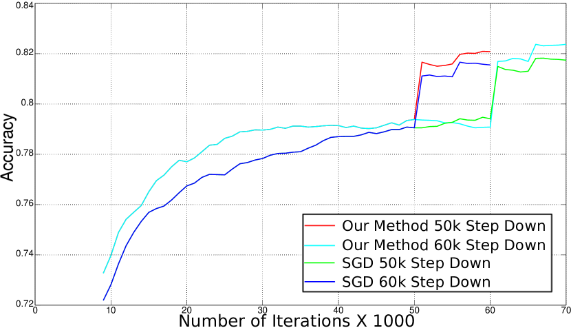
(a) Stochastic Gradient Descent

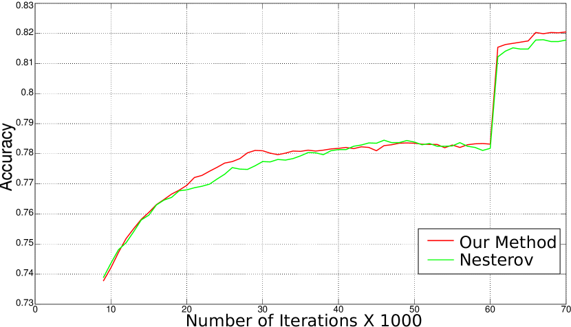
(b) Nesterov’s Accelerated Gradient

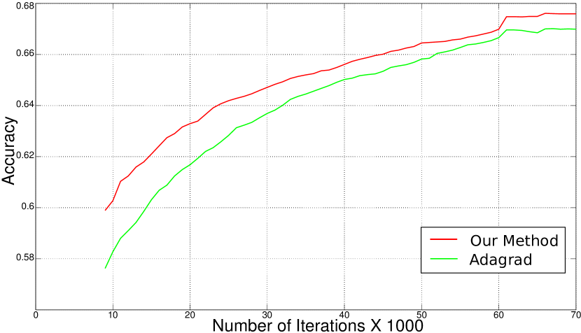
(c) AdaGrad

Figure 1: On CIFAR data set: plots showing accuracies (Figures 1(a)-1(c)) comparing SGD, NAG and AdaGrad, each with our adaptive layer-wise learning rates. For the SGD plot, we show results both when we step down the learning rate at 50,000 iterations as well as 60,000 iterations.

IV-A Dataset

We present image classification results on three standard datasets: MNIST, CIFAR10 and ImageNet (ILSVRC 2012 dataset, part of the ImageNet challenge). MNIST contains 60,000 handwritten digit images for training and 10,000 handwritten digit images for testing. CIFAR10 contains has 10 classes with 6,000 images in each class. ImageNet contains 1.2 million color images from 1000 different classes.

IV-B Experimental Details

We use Caffe [16] to implement our method. Caffe provides optimization methods for Stochastic Gradient Descent (SGD), Nesterov’s Accelerated Gradient (NAG) and AdaGrad. For a fair comparison between state-of-the-art methods, we add our adaptive layer-specific learning rate method on top of each of these optimization methods. In our experiments, we demonstrate the effectiveness of our algorithm on convolutional neural networks on 3 datasets. On CIFAR10, we use the same global learning rate as provided in Caffe. Since our method always increases the layer-specific learning rate (with respect to other optimization methods) based on the global learning rate, we start with a slightly smaller learning rate of 0.006 to make the learning less aggressive for the ImageNet experiment. SGD was initialized with the learning rate used in [2] for experiments done on ImageNet.

IV-B1 MNIST

We use the same architecture as LeNet for our experiments on MNIST. We present the results of using our proposed layer-specific learning rates on top of stochastic gradient descent, Nesterov’s accelerated gradient method and AdaGrad on the MNIST dataset. Since all methods converge very quickly on this dataset, we present the accuracy and loss only for the first 2,000 iterations. Table I shows the mean accuracy and standard deviation when each method was run 10 times. We observe that our proposed layer-specific learning rate is consistently better than Nesterov’s accelerated gradient, stochastic gradient descent and AdaGrad. In all the experiments, the proposed method also attains the maximum accuracy of 99.2% just like stochastic gradient descent, Nesterov’s accelerated gradient and AdaGrad.

IV-B2 CIFAR10

On CIFAR10 we use a convolutional neural network with 2 layers of 32 feature maps from $5\times 5$ convolution kernels, each followed by $3\times 3$ max pooling layers. After this we have another convolution layer with 64 feature maps from a $5\times 5$ convolution kernel followed by a $3\times 3$ max pooling layer. Finally, we have a fully connected layer with 10 hidden nodes and a soft-max logistic regression layer. After each convolution layer a ReLu non-linearity is applied. This is the same architecture as specified in Caffe. For the first 60,000 iterations the learning rate was 0.001 and it was dropped by a factor of 10 at 60,000 and 65,000 iterations.

Iteration	SGD	Ours-SGD	Nesterov	Ours-NAG	AdaGrad	Ours-AdaGrad
5000	68.8 $\pm$ 0.49	70.10 $\pm$ 0.89	69.36 $\pm$ 0.31	70.10 $\pm$ 0.59	54.90 $\pm$ 0.26	57.53 $\pm$ 0.67
10000	74.05 $\pm$ 0.51	74.48 $\pm$ 0.59	73.17 $\pm$ 0.25	74.00 $\pm$ 0.29	58.26 $\pm$ 0.58	60.95 $\pm$ 0.59
25000	77.40 $\pm$ 0.32	77.43 $\pm$ 0.15	76.17 $\pm$ 0.61	77.29 $\pm$ 0.59	63.02 $\pm$ 0.95	64.90 $\pm$ 0.57
60000	78.76 $\pm$ 0.87	78.74 $\pm$ 0.38	78.35 $\pm$ 0.33	78.18 $\pm$ 0.65	66.86 $\pm$ 0.93	68.03 $\pm$ 0.23
70000	81.78 $\pm$ 0.14	82.10 $\pm$ 0.32	81.75 $\pm$ 0.25	81.92 $\pm$ 0.26	67.04 $\pm$ 0.91	68.30 $\pm$ 0.39

TABLE II: Mean accuracy on CIFAR10 after different iterations for SGD, NAG and AdaGrad with their layer specific adaptive versions are shown in the table. The mean and standard deviation over 5 runs is reported.

On this dataset, we again observe that final error and loss of our method is consistently lower than SGD, NAG and AdaGrad (Table II). After step down, our adaptive method reaches a lower accuracy than both SGD and NAG. Note that just using our optimization method (without changing the network architecture) we can get an improvement of 0.32% over the mean accuracy for SGD. Even if we step down the learning rate at 50,000 iterations (taking 60000 iterations in total), we obtain an accuracy of 82.08%, which is better than SGD after 70,000 iterations, significantly cutting down on required training time Fig. 1. Since our method converges much faster when used with SGD, it is possible to perform the step down on the learning rate even earlier, potentially reducing training time even further. Although Adagrad does not perform very well on CIFAR10 with default parameters, we observe an improvement of 1.3% over the mean final accuracy, with again a significant speed-up in training time.

IV-B3 ImageNet

We use an implementation of AlexNet [2] in Caffe, a deep convolutional neural network architecture, for comparing our method with other optimization algorithms. AlexNet consists of 5 convolution layers followed by 3 fully connected layers. More details regarding the architecture can be found in the paper [2].

Since AlexNet is a deep neural network with significant complexity, it is suitable to apply our method on this network architecture. Fig 2 shows the results of using our method over SGD. We observe that our method obtains significantly greater accuracy and lower loss after 100,000 and 200,000 iterations. Further, we are also able to reach the maximum accuracy of 57.5% on the validation set after 295,000 iterations which is achieved by SGD only after 345,000 iterations, resulting in a reduction of 15% in training time. Given that such a large model takes more than a week to train properly, this is a significant reduction. Our loss is also consistently lower than SGD across all iterations. In the existing model, we perform a step down by a factor of 10 after every 100,000 iterations. In order to analyze how our method performs when we reduce the number of training iterations, we vary the number of training iterations at a specific learning rate before performing a step down. Table III shows the final accuracy after 350,000 iterations of SGD and our method. Although the final accuracy drops slightly as we decrease the number of iterations after which we perform the step down in the learning rate, it is clearly evident that our method achieves better accuracy than SGD. Note that we report top-1 class accuracy. Since we use the Caffe implementation of the AlexNet architecture and do not use any data augmentation techniques, our results are slightly lower than those reported in [2].

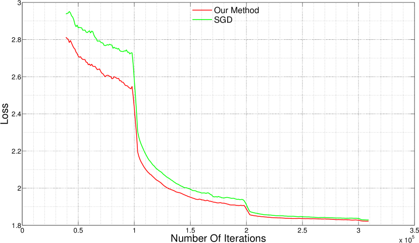
(a) Loss with Stochastic Gradient Descent

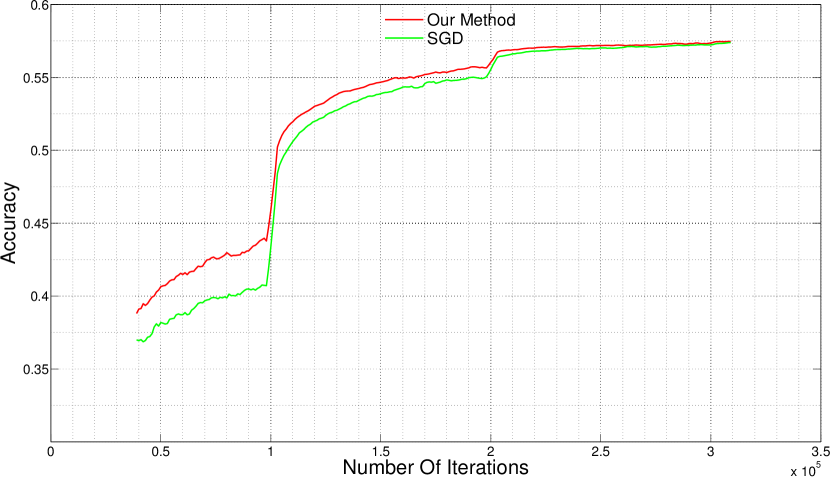
(b) Accuracy with Stochastic Gradient Descent

Figure 2: On ImageNet data set: plot comparing stochastic gradient descent with our adaptive layer-wise learning rates. We can see a consistent improvement in accuracy and loss over the regular SGD method across all iterations.

Iterations	SGD	Our Method
70,000	55.72%	55.84%
80,000	56.25%	56.57%
90,000	56.96%	57.13%

TABLE III: Comparison of stochastic gradient descent and Our Method with step-down at different iterations on ImageNet

V Conclusions

In this paper we propose a general method for training deep neural networks using layer-specific adaptive learning rates, which can be used on top of any optimization method with a global learning rate. The method uses gradients from each layer to compute an adaptive learning rate for each layer. It aims to speed up convergence when the parameters are in a low curvature saddle point region. Layer-specific learning rates also enable the method to prevent slow learning in initial layers of the deep network, usually caused by very small gradient values.

References

- [1] R. Pascanu, Y. N. Dauphin, S. Ganguli, and Y. Bengio, “On the saddle point problem for non-convex optimization,” arXiv preprint arXiv:1405.4604, 2014.
- [2] A. Krizhevsky, I. Sutskever, and G. E. Hinton, “Imagenet classification with deep convolutional neural networks,” in Advances in neural information processing systems, 2012, pp. 1097–1105.
- [3] Y. Taigman, M. Yang, M. Ranzato, and L. Wolf, “Deepface: Closing the gap to human-level performance in face verification,” in Computer Vision and Pattern Recognition (CVPR), 2014 IEEE Conference on. IEEE, 2014, pp. 1701–1708.
- [4] R. Socher, A. Perelygin, J. Y. Wu, J. Chuang, C. D. Manning, A. Y. Ng, and C. Potts, “Recursive deep models for semantic compositionality over a sentiment treebank,” in Proceedings of the Conference on Empirical Methods in Natural Language Processing (EMNLP). Citeseer, 2013, pp. 1631–1642.
- [5] G. Hinton, L. Deng, D. Yu, G. E. Dahl, A.-r. Mohamed, N. Jaitly, A. Senior, V. Vanhoucke, P. Nguyen, T. N. Sainath et al., “Deep neural networks for acoustic modeling in speech recognition: The shared views of four research groups,” Signal Processing Magazine, IEEE, vol. 29, no. 6, pp. 82–97, 2012.
- [6] X. Glorot, A. Bordes, and Y. Bengio, “Deep sparse rectifier networks,” in Proceedings of the 14th International Conference on Artificial Intelligence and Statistics. JMLR W&CP Volume, vol. 15, 2011, pp. 315–323.
- [7] H. Robbins, S. Monro et al., “A stochastic approximation method,” The Annals of Mathematical Statistics, vol. 22, no. 3, pp. 400–407, 1951.
- [8] M. D. Zeiler, “Adadelta: An adaptive learning rate method,” arXiv preprint arXiv:1212.5701, 2012.
- [9] J. Duchi, E. Hazan, and Y. Singer, “Adaptive subgradient methods for online learning and stochastic optimization,” The Journal of Machine Learning Research, vol. 12, pp. 2121–2159, 2011.
- [10] S. Hochreiter and J. Schmidhuber, “Long short-term memory,” Neural computation, vol. 9, no. 8, pp. 1735–1780, 1997.
- [11] A. J. Bray and D. S. Dean, “Statistics of critical points of gaussian fields on large-dimensional spaces,” Physical review letters, vol. 98, no. 15, p. 150201, 2007.
- [12] Y. V. Fyodorov and I. Williams, “Replica symmetry breaking condition exposed by random matrix calculation of landscape complexity,” Journal of Statistical Physics, vol. 129, no. 5-6, pp. 1081–1116, 2007.
- [13] B. T. Polyak, “Some methods of speeding up the convergence of iteration methods,” USSR Computational Mathematics and Mathematical Physics, vol. 4, no. 5, pp. 1–17, 1964.
- [14] Y. Nesterov, “A method of solving a convex programming problem with convergence rate o (1/k2),” in Soviet Mathematics Doklady, vol. 27, no. 2, 1983, pp. 372–376.
- [15] I. Sutskever, J. Martens, G. Dahl, and G. Hinton, “On the importance of initialization and momentum in deep learning,” in Proceedings of the 30th International Conference on Machine Learning (ICML-13), 2013, pp. 1139–1147.
- [16] Y. Jia, E. Shelhamer, J. Donahue, S. Karayev, J. Long, R. Girshick, S. Guadarrama, and T. Darrell, “Caffe: Convolutional architecture for fast feature embedding,” arXiv preprint arXiv:1408.5093, 2014.