A Critical Survey of Deconvolution Methods for Separating cell-types in Complex Tissues

Abstract

Identifying properties and concentrations of components from an observed mixture, known as deconvolution, is a fundamental problem in signal processing. It has diverse applications in fields ranging from hyperspectral imaging to denoising readings from biomedical sensors. This paper focuses on in-silico deconvolution of signals associated with complex tissues into their constitutive cell-type specific components, along with a quantitative characterization of the cell-types. Deconvolving mixed tissues/cell-types is useful in the removal of contaminants (e.g., surrounding cells) from tumor biopsies, as well as in monitoring changes in the cell population in response to treatment or infection. In these contexts, the observed signal from the mixture of cell-types is assumed to be a convolution, using a linear instantaneous (LI) mixing process, of the expression levels of genes in constitutive cell-types. The goal is to use known signals corresponding to individual cell-types along with a model of the mixing process to cast the deconvolution problem as a suitable optimization problem.

In this paper, we present a survey and in-depth analysis of models, methods, and assumptions underlying deconvolution techniques. We investigate the choice of the different loss functions for evaluating estimation error, constraints on solutions, preprocessing and data filtering, feature selection, and regularization to enhance the quality of solutions, along with the impact of these choices on the performance of commonly used regression-based methods for deconvolution. We assess different combinations of these factors and use detailed statistical measures to evaluate their effectiveness. Some of these combinations have been proposed in the literature, whereas others represent novel algorithmic choices for deconvolution. We identify shortcomings of current methods and avenues for further investigation. For many of the identified shortcomings, such as normalization issues and data filtering, we provide new solutions. We summarize our findings in a prescriptive step-by-step process, which can be applied to a wide range of deconvolution problems.

1 Introduction

Source separation, or deconvolution, is the problem of estimating individual signal components from their mixtures. This problem arises when source signals are transmitted through a mixing channel and the mixed sensor readings are observed. Source separation has applications in a variety of fields. One of its early applications was in processing audio signals [10, 11, 12, 13]. Here, mixtures of different sound sources, such as speech or music, are recorded simultaneously using several microphones. Various frequencies are convolved by the impulse response of the room and the goal is to separate one or several sources from this mixture. This has direct applications in speech enhancement, voice removal, and noise cancellation in recordings from populated areas. In hyperspectral imaging, the spectral signature of each pixel is observed. This signal is the combination of pure spectral signatures of constitutive elements mixed according to their relative abundance. In satellite imaging, each pixel represents sensor readings for different patches of land at multiple wavelengths. Individual sources correspond to reflectances of materials at different wavelengths that are mixed according to the material composition of each pixel [1, 2, 3, 4, 5].

Beyond these domains, deconvolution has applications in denoising biomedical sensors. Tracing electrical current in the brain is widely used as a proxy for spatiotemporal patterns of brain activity. These patterns have significant clinical applications in diagnosis and prediction of epileptic seizures, as well as characterizing different stages of sleep in patients with sleep disorders. Electroencephalography (EEG) and magnetoencephalography (MEG) are two of the most commonly used techniques for cerebral imaging. These techniques measure voltage fluctuations and changes in the electromagnetic fields, respectively. Superconducting QUantum Interference Device (SQUID) sensors used in the latter technology are susceptible to magnetic coupling due to geometry and must be shielded carefully against magnetic noise. Deconvolution techniques are used to separate different noise sources and ameliorate the effect of electrical and magnetic coupling in these devices [6, 7, 8, 9].

At a high level, mixing channels can be classified as follows: (i) linear or nonlinear, (ii) instantaneous, delayed, or convolutive, and (iii) over/under determined. When neither the sources nor the mixing process is available, the problem is known as blind source separation (BSS). This problem is highly under-determined in general, and additional constraints; such as independence among sources, sparsity, or non-negativity; are typically enforced on the sources in practical applications. On the other hand, a new class of methods has been developed recently, which is known as semi or guided BSS [10, 7, 12, 13]. In these methods, additional information is available a priori on the approximate behavior of either sources or the mixing process. In this paper, we focus on the class of over-determined, linear instantaneous (LI) mixing processes, for which a deformed prior on sources is available. In this case, the parameters of the linear mixer, as well as the true identity of the original sources are to be determined.

In the context of molecular biology, deconvolution methods have been used to identify constituent cell-types in a tissue, along with their relative proportions. The inherent heterogeneity of tissue samples makes it difficult to identify separated, cell-type specific signatures, i.e., the precise gene expression levels for each cell-type. Relative changes in cell proportions, combined with variations attributed to the changes in the biological conditions, such as disease state, complicate identification of true biological signals from mere technical variations. Changes in tissue composition are often indicative of disease progression or drug response. For example, coupled depletion of specific neuronal cells with the gradual increase in the glial cell population is indicative of neurodegenerative disorders. An increasing proportion of malignant cells, as well as a growing fraction of tumor infiltrating lymphocytes (TIL) compared to surrounding cells, directly influence tumor growth, metastasis, and clinical outcomes for patients [14, 15]. Deconvolving tissue biopsies allows further investigation of the interaction between tumor and micro-environmental cells, along with its role in the progression of cancer.

The expression level of genes, which is a proxy for the number of present copies of each gene product, is one of the most common source factors used for separating cell-types and tissues. In the linear mixing model, the expression of each gene in a complex mixture is estimated as a linear combination of the expression of the same gene in the constitutive cell-types. In silico deconvolution methods for separating complex tissues can be coarsely classified as either full deconvolution, in which both cell-type specific expressions and the percentages of each cell-type are estimated, or partial deconvolution methods, where one of these data sources is used to compute the other [16]. These two classes loosely relate to BSS and guided-BSS problems. Note that in cases where relative abundances are used to estimate cell-type-specific expressions, the problem is highly under-determined, whereas in the complementary case of computing percentages from noisy expressions of purified cells, it is highly over-determined. The challenge is to select the most reliable features that satisfy the linearity assumption. We provide an in-depth review of the recent deconvolution methods in Section 2.5.

In contrast to computational methods, a variety of experimental cell separation techniques have been proposed to enrich samples for cell-types of interest. However, these experimental methods not only involve significant time, effort, and expense, but may also result in insufficient RNA abundance for further quantification of gene expression. In this case, amplification steps may introduce technical artifacts into the gene expression data. Furthermore, sorting of cell-types must be embedded in the experiment design for the desired subset of cells, and any subsequent separation is infeasible. Computational methods, on the other hand, are capable of sorting mixtures at different levels of resolution and for arbitrary cell-type subsets of interest.

The organization of the remainder of the paper is as follows: in Section 2.1 we introduce the basic terminology from biology needed to formally define the deconvolution problem in the context of quantifying cell-type fractions in complex tissues. The formal definition of the deconvolution problem and its relationship to linear regression is defined in Section 2.2. Sections 2.3 and 2.4 review different choices and examples of the objective function used in regression. An overview of computational methods for biological deconvolution is provided in Section 2.5. Datasets and evaluation measures used in this study are described in Sections 3.1 and 3.2, respectively. The effect of the loss function, constraint enforcement, range filtering, and feature selection choices on the performance of deconvolution methods is evaluated systematically in Sections 3.4-3.8. Finally, a summary of our findings is provided in Section 4.

2 Background and Notation

2.1 Biological Underpinnings

The central dogma of biology describes the flow of genetic information within cells – the genetic code, represented in DNA molecules, is first transcribed to an intermediate construct, called messenger RNA (mRNA), which in turn translates into proteins. These proteins are the functional workhorses of the cell. Genes, defined as the minimal coding sections of the DNA, contain the recipe for making proteins. These instructions are utilized dynamically by the cell to adapt to different conditions. The amounts of various proteins in a cell can be measured at a time point. This corresponds to the level of protein expression. This process is limited by the availability of high-quality antibodies that can specifically target each protein. The amount of active mRNA in a cell, however, can be measured at the genome scale using high-throughput technologies such as microarrays and RNASeq. The former is an older technology that relies on the binding affinity of complementary base pairs (alphabets used in the DNA/RNA molecules), while the latter is a newer technique, using next generation sequencing (NGS). This technique estimates gene expression based on the overlap of mRNA fragments with known genomic features. Since microarrays have been used for years, extensive databases from different studies are publicly available. RNASeq datasets, in comparison, are relatively smaller but growing rapidly in scale and coverage. Both of these technologies provide reliable proxies for the amount of proteins in cells, with RNASeq being more sensitive, especially for lowly expressed genes. A drawback of these methods, however, is that the true protein expression is also regulated by additional mechanisms, such as post-transcriptional modifications, which cannot be assayed at the mRNA level.

The expression level of genes is tightly regulated in different stages of cellular development and in response to environmental changes. In addition to these biological variations due to cellular state, intermediate steps in each technology introduce technical variations in repeated measurement of gene expression in the same cell-type. To enhance reproducibly of measurements, one normally includes multiple instances of the same cell-type in each experiment, known as technical replicates. The expression profiles from these experiments provide a snapshot of the cell under different conditions. In addition to biological variation of genes within the same cell-type, there is an additional level of variation when we look across different cell-types. Some genes are ubiquitously expressed in all cell-types to perform housekeeping functions, whereas other genes exhibit specificity or selectivity for one, or a group of cell-types, respectively. A compendium of expression profiles of different cells at different developmental stages is the data substrate for in silico deconvolution of complex tissues.

2.2 Deconvolution: Formal Definition

We introduce formalisms and notation used in discussing different aspects of in silico deconvolution of biological signals. We focus on models that assume linearity, that is, the expression signature of the mixture is a weighted sum of the expression profile for its constitutive cell-types. In this case, sources are cell-type specific references and the mixing process is determined by the relative fraction of cell-types in the mixture.

We first introduce the mathematical constructs used:

• $\mathbf{M}\in\mathbb{R}^{n\times p}$: Mixture matrix, where each entry $\mathbf{M}(i,j)$ represents the raw expression of gene $i$, $1\leq i\leq n$, in heterogeneous sample $j$, $1\leq j\leq p$. Each sample, represented by $\boldsymbol{m}$, is a column of the matrix $\mathbf{M}$, and is a combination of gene expression profiles from constituting cell types in the mixture.

• $\mathbf{H}\in\mathbb{R}^{n\times r}$: Reference signature matrix for the expression of primary cell types, with multiple biological/technical replicates for each cell-type. In this matrix, rows correspond to the same set of genes as in $\mathbf{M}$, columns represent replicates and there is an underlying grouping among columns that collects profiles corresponding to the same cell-type.

• $\mathbf{G}\in\mathbb{R}^{n\times q}$: Reference expression profile, where the expression of similar cell-types in matrix $\mathbf{H}$ is represented by the average value.

• $\mathbf{C}\in\mathbb{R}^{q\times p}$: Relative proportions of each cell-type in the mixture sample. Here, rows correspond to cell-types and columns represent samples in mixture matrix $\mathbf{M}$.

Using this notation, we can formally define deconvolution as an optimization problem that seeks to identify “optimal” estimates for matrices $\mathbf{G}$ and $\mathbf{C}$, denoted by $\hat{\mathbf{G}}$ and $\hat{\mathbf{C}}$, respectively. Since $\mathbf{G}$ and/or $\mathbf{C}$ are not known a priori, we use an approximation that is based on the linearity assumption. In this case, we aim to find $\hat{\mathbf{G}}$ and $\hat{\mathbf{C}}$ such that their product is close to the mixture matrix, $\mathbf{M}$. Specifically, given a function $\boldsymbol{\delta}$ that measures the distance between the true and approximated solutions, also referred to as the loss function, we aim to solve:

$$\min_{0\leq\hat{\mathbf{G}},\hat{\mathbf{C}}}\boldsymbol{\delta}(\hat{\mathbf{G}}\hat{\mathbf{C}},\mathbf{M})$$ (1)

In partial deconvolution, either $\mathbf{C}$ or $\mathbf{G}$, or their noisy representation, is known a priori and the goal is to find the other unknown matrix. When matrix $\mathbf{G}$, referred to as the reference profile, is known, the problem is over-determined and we seek to distinguish features (genes) that closely conform to the linearity assumption, from the rest of the (variable) genes. In this case, we can solve the problem individually for each mixture sample. Let us denote by $\boldsymbol{m}$ and $\hat{\boldsymbol{c}}$ the expression profile and estimated cell-type proportion of a mixture sample, respectively. Then, we can rewrite Equation 1 as:

$$\min_{0\leq\hat{\boldsymbol{c}}}\boldsymbol{\delta}(\mathbf{G}\hat{\boldsymbol{c}},\boldsymbol{m})$$ (2)

This formulation is essentially a linear regression problem, with an arbitrary loss function. On the other hand, in the case of full deconvolution, we can still estimate $\mathbf{C}$ in a column-by-column fashion. However, estimating $\mathbf{G}$ is highly under-determined and we must use additional sources to restrict the search space. One such source of information is the variation across samples in $\mathbf{M}$, depending on the cell-type concentrations in the latest estimated value of $\mathbf{C}$. In general, most regression-based methods for full deconvolution use an iterative scheme that starts from either noisy estimates of $\mathbf{G}$ and $\mathbf{C}$, or a random sample that satisfies given constraints on these matrices, and successively improves over this initial approximation. This iterative process can be formalized as follows:

$$\hat{\mathbf{C}} \leftarrow \operatorname*{\boldsymbol{\arg}\!\boldsymbol{\min}}\limits_{0\leq\hat{\mathbf{C}}}(\boldsymbol{\delta}(\hat{\mathbf{G}}\hat{\mathbf{C}}-\mathbf{M}))$$ (3)

$$\hat{\mathbf{G}} \leftarrow (\operatorname*{\boldsymbol{\arg}\!\boldsymbol{\min}}\limits_{0\leq\hat{\mathbf{G}}}(\boldsymbol{\delta}(\hat{\mathbf{C}}^{T}\hat{\mathbf{G}}^{T}-\mathbf{M})^{T}))^{T}$$

Please note that the updating $\hat{\mathbf{G}}$ is typically row-wise (for each gene), whereas updation of $\hat{\mathbf{C}}$ is column-wise (for each sample). Non-negative matrix factorization (NMF) is a dimension reduction technique that aims to factor each column of the given input matrix as a nonnegative weighted sum of non-negative basis vectors, with the number of basis vectors being equal or less than the number of columns in the original matrix. The alternating non-negative least squares formulation (ANLS) for solving NMF can be formulated using the framework introduced in Equation 3. There are additional techniques for solving NMF, including the multiplicative updating rule and the hierarchical alternating least squares (HALS) methods, all of which are special cases of block-coordinate descent [25]. Two of the most common loss functions used in NMF are the Frobenius and Kullback-Leibler (KL) divergence [25].

In addition to non-negativity (NN), an additional sum-to-one (STO) constraint is typically applied over columns of the matrix $\hat{\mathbf{C}}$, or the sample-specific vector $\hat{\boldsymbol{c}}$. This constraint restricts the search space, which can potentially enhance the accuracy of the results, and simplifies the interpretation of values in $\hat{\boldsymbol{c}}$ as relative percentages. Finally, another fundamental assumption that is mostly neglected in prior work is the similar cell quantity (SCQ) constraint. The similar cell quantity assumption states that all reference profiles and corresponding mixtures must be normalized to ensure that they represent the expression level of the “same number of cells.” If this constraint is not satisfied, differences in the cell-type counts directly affect concentrations by rescaling the estimated coefficients to adjust for the difference.

In this paper, we focus on different loss functions ($\boldsymbol{\delta}$ functions), as well as the role of constraint enforcement strategies, in estimating $\hat{\boldsymbol{c}}$. These constitute the key building blocks of both partial and full deconvolution methods.

2.3 Choice of Objective Function

In linear regression, often a slightly different notation is used, which we describe here. We subsequently relate it to the deconvolution problem. Given a set of samples, $\{(\boldsymbol{x}_{i},y_{i})\}_{i=1}^{m}$, where $\boldsymbol{x}_{i}\in\mathbb{R}^{k}$ and $y_{i}\in\mathbb{R}$, the regression problem seeks to find a function $f(\boldsymbol{x})$ that minimizes the aggregate error over all samples. Let us denote the fitting error by $r_{i}=y_{i}-f(\boldsymbol{x}_{i})$. Using this notation, we can write the regression problem as:

$$\operatorname*{\boldsymbol{\arg}\!\boldsymbol{\min}}_{f\in\mathcal{F}}\sum_{i=1}^{m}\boldsymbol{\mathcal{L}}(r_{i})$$ (4)

where the loss function $\boldsymbol{\mathcal{L}}$ measures the cost of estimation error. We focus on the class of linear functions, that is $f_{\boldsymbol{w}}(\boldsymbol{x})=\boldsymbol{w}^{T}\boldsymbol{x}$, for which we have $r_{i}=y_{i}-\boldsymbol{w}^{T}\boldsymbol{x}_{i}$. In this formulation, $y_{i}$ corresponds to the expression level of a gene in the mixture, vector $\boldsymbol{x}_{i}$ is the expression level of the same gene in the reference cell types, and $\boldsymbol{w}$ is the fraction of each cell-type in the mixture. We can represent $\{\boldsymbol{x}_{i}\}_{i=1}^{m}$ in the compact form by matrix $\mathbf{X}$, in which row $i$ corresponds to $\boldsymbol{x}_{i}$.

In cases where the number of parameters is greater than the number of samples, that is matrix $\mathbf{X}$ is a fat matrix, minimizing Equation 4, directly, can result in the over-fitting problem. Furthermore, when features (columns of $\mathbf{X}$) are highly correlated, solution may change drastically in response to small changes in the samples, specifically among the correlated features. This condition, known as multicollinearity, can result in inaccurate estimates, in which coefficients of similar features are greatly different. To remedy these problems, we can add a regularization term, which incorporates additional constraints (such as sparsity or flatness) to enhance the stability of results. We re-write the problem with the added regularizer as:

$$\operatorname*{\boldsymbol{\arg}\!\boldsymbol{\min}}_{\boldsymbol{w}\in\mathbb{R}^{k}}\{\underbrace{\sum_{i=1}^{m}\boldsymbol{\mathcal{L}}(y_{i}-\boldsymbol{w}^{T}\boldsymbol{x}_{i})}_{\mbox{Overall loss}}+\underbrace{\lambda\boldsymbol{\mathcal{R}}(\boldsymbol{w})}_{\mbox{Regularizer}}\}$$ (5)

where the $\lambda$ parameter controls the relative importance of estimation error versus regularization. There are different choices and combinations for the loss function $\boldsymbol{\mathcal{L}}$ and regularizer function $\boldsymbol{\mathcal{R}}$, which we describe in the following sections.

2.3.1 Choice of Loss Functions

There are a variety of options for suitable loss functions. Some of these functions are known to be asymptotically optimal for a given noise density, whereas others may yield better performance in practice when assumptions underlying the noise model are violated. We summarize the most commonly used set of loss functions:

• If we assume that the underlying model is perturbed by Gaussian white noise, the squared or quadratic loss, denoted by $\boldsymbol{\mathcal{L}}_{2}$, is known to be asymptotically optimal. This loss function is used in classical least squares regression and is defined as:

  $$\boldsymbol{\mathcal{L}}_{2}(r_{i})=r_{i}^{2}=(y_{i}-\boldsymbol{w}^{T}\boldsymbol{x}_{i})^{2}$$

• Absolute deviation loss, denoted by $\boldsymbol{\mathcal{L}}_{1}$, is the optimal choice if noise follows a Laplacian distribution. Formally, it is defined as:

  $$\boldsymbol{\mathcal{L}}_{1}(r_{i})=|r_{i}|=|y_{i}-\boldsymbol{w}^{T}\boldsymbol{x}_{i}|$$

  Compared to $\boldsymbol{\mathcal{L}}_{2}$, the choice of $\boldsymbol{\mathcal{L}}_{1}$ is preferred in the presence of outliers, as it is less sensitive to extreme values

• Huber’s loss function, denoted by $\boldsymbol{\mathcal{L}}_{huber}^{(M)}$, is a parametrized combination of $\boldsymbol{\mathcal{L}}_{1}$ and $\boldsymbol{\mathcal{L}}_{2}$. The main idea is that $\boldsymbol{\mathcal{L}}_{2}$ loss is more susceptible to outliers, while it is more sensitive to small estimation errors. To combine the best of these two functions, we can define a half-length parameter $M$, which we use to transition from $\boldsymbol{\mathcal{L}}_{2}$ to $\boldsymbol{\mathcal{L}}_{1}$. More formally:

  $$\boldsymbol{\mathcal{L}}_{Huber}^{(M)}(r_{i})=\begin{cases}r_{i}^{2},&\mbox{if $|r_{i}|\leq M$}\\ M(2|r_{i}|-M),&\mbox{otherwise}\end{cases}$$

• The loss function used in support vector regression (SVR) is the $\epsilon$-insensitive loss, denoted by $\boldsymbol{\mathcal{L}}_{\epsilon}^{(\epsilon)}$. Similar to Huber loss, there is a transition phase between small and large estimation errors. However, $\epsilon$-insensitive loss does not penalize the errors that are smaller than a threshold. Formally, we define $\epsilon$-insensitive loss as:

  $$\boldsymbol{\mathcal{L}}_{\epsilon}^{(\epsilon)}(r_{i}) = \boldsymbol{\max}(0,|r_{i}|-\epsilon)$$

  $$= \begin{cases}0,&\mbox{if $|r_{i}|\leq\epsilon$}\\ |r_{i}|-\epsilon,&\mbox{otherwise}\end{cases}$$

Figure 1 provides a visual representation of these loss functions, in which we use $M=1$ and $\epsilon=\frac{1}{2}$ for the Huber and $\epsilon$-insensitive loss functions, respectively. Note that for small residual values, $|r_{i}|\leq M=1$, Huber and square loss are equivalent. However, outside this region Huber loss becomes linear.

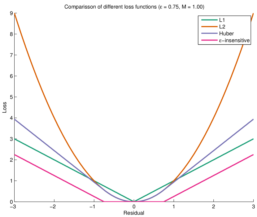
Figure 1: Comparison of different loss functions

2.3.2 Choice of Regularizers

When the reference profile contains many cell-types that may not exist in mixtures, or in cases where constitutive cell-types are highly correlated, regularizing the objective function can sparsify the solution or enhance the conditioning of the problem. We describe two commonly used regularizers here:

• The norm-2 regularizer is used to shrink the regression coefficient vector $\boldsymbol{w}$ to ensure that it is as flat as possible. A common use of this regularizer is in conjunction with $\boldsymbol{\mathcal{L}}_{2}$ loss to remedy the multi-collinearity problem in classical least squares regression. This regularizer is formally defined as:

  $$\boldsymbol{\mathcal{R}}_{2}(\boldsymbol{w})=\parallel\boldsymbol{w}\parallel_{2}^{2}=\sum_{i=1}^{k}w_{i}^{2}.$$ (6)

• Another common regularizer is the norm-1 regularizer, which is used to enforce sparsity over $\boldsymbol{w}$. Formally, it can be defined as:

  $$\boldsymbol{\mathcal{R}}_{1}(\boldsymbol{w})=\parallel\boldsymbol{w}\parallel_{1}=\sum_{i=1}^{k}|w_{i}|.$$ (7)

In addition to these two regularizers, their combinations have also been introduced in the literature. One such example is elastic net, which uses a convex combination of the two, that is $\boldsymbol{\mathcal{R}}_{elastic}(\boldsymbol{w})=\alpha\boldsymbol{\mathcal{R}}_{1}(\boldsymbol{w})+(1-\alpha)\boldsymbol{\mathcal{R}}_{2}(\boldsymbol{w})$. Another example is group Lasso, which, given a grouping $G$ among cell-types, enforces flatness among members of the group, while enhancing the sparsity pattern across groups. This regularizer function can be written as $\boldsymbol{\mathcal{R}}_{group}=\sum_{G_{i}}\boldsymbol{\mathcal{L}}_{2}(\boldsymbol{w}(G_{i}))$, where $\boldsymbol{w}(G_{i})$ is the weight of cell-types in the $i^{th}$ group.

2.4 Examples of objective functions used in practice

2.4.1 Ordinary Least Squares (OLS)

The formulation of OLS is based on squared loss, $\boldsymbol{\mathcal{L}}_{2}$. Formally, we have:

$$\boldsymbol{\min}_{\boldsymbol{w}}\{\sum_{i=1}^{m}\boldsymbol{\mathcal{L}}_{2}(r_{i})\} = \boldsymbol{\min}_{\boldsymbol{w}}\{\sum_{i=1}^{m}(y_{i}-\boldsymbol{w}^{T}\boldsymbol{x}_{i})^{2}\}$$

$$= \boldsymbol{\min}_{\boldsymbol{w}}\parallel y-\mathbf{X}\boldsymbol{w}\parallel_{2}^{2}$$

where row $i$ of the matrix $\mathbf{X}$, also known as the design matrix, corresponds to $\boldsymbol{x}_{i}$. This formulation has a closed form solution given by:

$$\hat{\boldsymbol{w}}=(\mathbf{X}^{T}\mathbf{X})^{-1}\mathbf{X}^{T}\boldsymbol{y}$$

In this formulation, we can observe that norm-2 regularization is especially useful in cases where the matrix $\mathbf{X}$ is ill-conditioned and near-singular, that is, columns are dependent on each other. By shifting $\mathbf{X}^{T}\mathbf{X}$ towards the identity matrix, we ensure that the eigenvalues are farther from zero, which enhances the conditioning of the resulting combination.

2.4.2 Ridge Regression

One of the main issues with the OLS formulation is that the design matrix, $\mathbf{X}$, should have full column rank $k$. Otherwise, if we have highly correlated variables, the solution suffers from the multicollinearity problem. This condition can be remedied by incorporating a norm-2 regularizer. The resulting formulation, known as ridge regression, is as follows:

$$\boldsymbol{\min}_{\boldsymbol{w}}\{\sum_{i=1}^{m}\boldsymbol{\mathcal{L}}_{2}(r_{i})+\lambda\boldsymbol{\mathcal{R}}_{2}(\boldsymbol{w})\}$$

$$=\boldsymbol{\min}_{\boldsymbol{w}}\parallel y-\mathbf{X}\boldsymbol{w}\parallel_{2}^{2}+\lambda\parallel\boldsymbol{w}\parallel_{2}^{2}$$

Similar to OLS, we can differentiate w.r.t. $\boldsymbol{w}$ to find the close form solution for Ridge regression given by:

$$\hat{\boldsymbol{w}}=(\mathbf{X}^{T}\mathbf{X}+\lambda\mathbf{I})^{-1}\mathbf{X}^{T}\boldsymbol{y}$$

2.4.3 Least Absolute Selection and Shrinkage Operator (LASSO) Regression

Combining the OLS with a norm-1 regularizer, we have the LASSO formulation:

$$\boldsymbol{\min}_{\boldsymbol{w}}\{\sum_{i=1}^{m}\boldsymbol{\mathcal{L}}_{2}(r_{i})+\lambda\boldsymbol{\mathcal{R}}_{1}(\boldsymbol{w})\}$$

$$=\boldsymbol{\min}_{\boldsymbol{w}}\parallel y-\mathbf{X}\boldsymbol{w}\parallel_{2}^{2}+\lambda\parallel\boldsymbol{w}\parallel_{1}$$

This formulation is especially useful for producing sparse solutions by introducing zero elements in vector $\boldsymbol{w}$. However, while being convex, it does not have a closed form solution.

2.4.4 Robust Regression

It is known that $\boldsymbol{\mathcal{L}}_{2}(\boldsymbol{r})$ is dominated by the largest elements of the residual vector $\boldsymbol{r}$, which makes it sensitive to outliers. To remedy this problem, different robust regression formulations have been proposed that use alternative loss functions. Two of the best-known formulations are based on the $\boldsymbol{\mathcal{L}}_{1}$ and $\boldsymbol{\mathcal{L}}_{huber}$ loss functions. The $\boldsymbol{\mathcal{L}}_{1}$ formulation can be written as:

$$\boldsymbol{\min}_{\boldsymbol{w}}\{\sum_{i=1}^{m}\boldsymbol{\mathcal{L}}_{1}(r_{i})\} = \boldsymbol{\min}_{\boldsymbol{w}}\{\sum_{i=1}^{m}|y_{i}-\boldsymbol{w}^{T}\boldsymbol{x}_{i}|\}$$

$$= \boldsymbol{\min}_{\boldsymbol{w}}\parallel y-\mathbf{X}\boldsymbol{w}\parallel_{1}$$

However, for the Huber loss function, while it can be defined similarly, it is usually formulated as an alternative convex Quadratic Program (QP):

$$\boldsymbol{\min}_{\boldsymbol{x},\boldsymbol{z},\boldsymbol{t}} \{\frac{1}{2}\parallel\boldsymbol{z}\parallel_{2}^{2}+M\boldsymbol{1}^{T}\boldsymbol{t}\}$$

Subject to: $$-\boldsymbol{t}\leq\mathbf{X}\boldsymbol{w}-\boldsymbol{y}-\boldsymbol{z}\leq\boldsymbol{t}$$ (8)

which can be solved more efficiently using the following equivalent QP variant [17]:

$$\boldsymbol{\min}_{\boldsymbol{x},\boldsymbol{z},\boldsymbol{r},\boldsymbol{s}} \{\frac{1}{2}\parallel\boldsymbol{z}\parallel_{2}^{2}+M\boldsymbol{1}^{T}(\boldsymbol{r}+\boldsymbol{s})\}$$

Subject to: $$\begin{cases}\mathbf{X}\boldsymbol{w}-\boldsymbol{y}-\boldsymbol{z}=\boldsymbol{r}-\boldsymbol{s}&\\ 0\leq\boldsymbol{r},\boldsymbol{s}\end{cases}$$ (9)

In both of these formulations, the scalar $M$ corresponds to half-length parameter of the Huber’s loss function.

2.4.5 Support Vector Regression

In machine learning, Support Vector Regression (SVR) is a commonly used technique that aims to find a regression by maximizing the margins around the estimated separator hyperplane from the closest data points on each side of it. This margin provides the region in which estimation errors are ignored. SVR has been recently used to deconvolve biological mixtures, where it has been shown to outperform other methods [15]. One of the variants of SVR is $\epsilon$-SVR, in which parameter $\epsilon$ defines the margin, or the $\epsilon$-tube. The primal formulation of $\epsilon$-SVR with linear kernel can be written as [18]:

$$\boldsymbol{\min}_{\boldsymbol{w},\boldsymbol{\xi}^{+}_{i},\boldsymbol{\xi}^{-}_{i}} \{\frac{1}{2}\parallel\boldsymbol{w}\parallel_{2}^{2}+C\sum_{i=1}^{m}(\boldsymbol{\xi}_{i}^{+}+\boldsymbol{\xi}^{-}_{i})\}$$

Subject to: $$\begin{cases}y_{i}-\boldsymbol{w}\cdot\boldsymbol{x}_{i}\leq\epsilon+\boldsymbol{\xi}_{i}^{+}&\\ -(\epsilon+\boldsymbol{\xi}^{-}_{i})\leq y_{i}-\boldsymbol{w}\cdot\boldsymbol{x}_{i}&\\ 0\leq\boldsymbol{\xi}_{i}^{+},\boldsymbol{\xi}^{-}_{i}&\end{cases}$$ (10)

in which, given the unit norm assumption introduced in Section 2.2, we assume that $b=0$. The dual problem for the primal in Equation 10 can be written in matrix form as:

$$\boldsymbol{\max}_{\boldsymbol{\alpha}^{+},\boldsymbol{\alpha}^{-}} \Big{\{}\boldsymbol{1}^{T}\big{(}(\boldsymbol{\alpha}^{+}-\boldsymbol{\alpha}^{-})\odot\boldsymbol{y}\big{)}$$ (11)

$$-\epsilon\boldsymbol{1}^{T}(\boldsymbol{\alpha}^{+}+\boldsymbol{\alpha}^{-})$$

$$-(\boldsymbol{\alpha}^{+}-\boldsymbol{\alpha}^{-})^{T}\mathbf{K}(\boldsymbol{\alpha}^{+}-\boldsymbol{\alpha}^{-})\Big{\}}$$

$$\mbox{Subject to:}\begin{cases}\boldsymbol{1}^{T}(\boldsymbol{\alpha}^{+}-\boldsymbol{\alpha}^{-})=0&\\ 0\leq\boldsymbol{\alpha}^{+},\boldsymbol{\alpha}^{-}\leq C\end{cases}$$

In this formulation, $\boldsymbol{1}$ is a vector of all ones, $\odot$ is the element-wise product, and $\mathbf{K}$ is the kernel matrix defined as $\mathbf{K}=\mathbf{X}\mathbf{X}^{T}$. The dual formulation is often used to solve $\epsilon$-SVR, because it can be easily extended to use different kernel functions to map $\boldsymbol{x}_{i}$ to a $d$-dimensional non-linear feature space. Additionally, when $m\ll k$, such as the case of high-dimensional feature spaces, it provides a better way to solve the SVR problem. However, the primal problem provides a more straightforward interpretation. In addition, in the case where $k\ll m$, it provides superior performance. To show the similarity with Equation 5, we can rewrite Equation 10 using the $\epsilon$-insensitive loss function as follows:

$$\boldsymbol{\min}_{\boldsymbol{w}}\{\sum_{i=1}^{m}\mathcal{L}_{\epsilon}(y_{i}-\boldsymbol{w}^{T}\boldsymbol{x}_{i})+\lambda\boldsymbol{\mathcal{R}}_{2}(\boldsymbol{w})\}$$ (12)

where $\lambda=\frac{1}{2C}$ [19].

2.5 Overview of Prior in silico Deconvolution Methods

A majority of existing deconvolution methods fall into two groups – they either use a regression-based framework to compute $\mathbf{G}$, $\mathbf{C}$, or both; or perform statistical inference over a probabilistic model. Abbas et al. [20] present one of the early regression-based methods for estimating $\mathbf{C}$. This method is designed to identify cell-type concentrations from a known reference profile of immune cells. Their method is based on Ordinary Least Squares (OLS) regression and does not consider either non-negativity or sum-to-one constraints explicitly, but rather it enforces these constraints implicitly after the optimization procedure. An extension of this approach is proposed by Qiao et al. [21], which uses non-negative least squares (NNLS) to explicitly enforce non-negativity as part of the optimization. Gong et al. [22] present a quadratic programming (QP) framework to explicitly encode both constraints in the optimization problem formulation. They also propose an extension to this method, called DeconRNASeq, which applies the same QP framework to RNASeq datasets. More recently Newman et al. [15] propose robust linear regression (RLR) and $\nu$-SVR regression instead of $\boldsymbol{\mathcal{L}}_{2}$ based regression, which is highly susceptible to noise. Digital cell quantification (DCQ) [23] is another approach designed for monitoring the immune system during infection. Compared to prior methods, DCQ forces sparsity by combining $\boldsymbol{\mathcal{R}}_{2}$ and $\boldsymbol{\mathcal{R}}_{1}$ regularization into an elastic net. This regularization is essential for successfully identifying the subset of active cells at each stage, given the larger number of cell-types included in their panel (213 immune cell sub-populations). In contrast to these techniques, Shen-Orr et al. [24] propose a method, call csSAM, which is specifically designed to identify genes that are differentially expressed among purified cell-types. The core of this method is regression over matrix $\mathbf{C}$ to estimate matrix $\mathbf{G}$.

Full regression-based methods use variations of block-coordinate descent to successively identify better estimates for both $\mathbf{C}$ and $\mathbf{G}$ [25]. Venet et al. [26] present one of the early methods in this class, which uses an NMF-like method coupled with a heuristic to decorrelate columns of $\mathbf{G}$ in each iteration. Repsilber et al. [27] propose an algorithm called deconf, which uses alternating non-negative least squares (ANLS) for solving NMF, without the decorrelation step of Vennet et al., while implicitly applying constraints on $\mathbf{C}$ and $\mathbf{G}$ at each iteration. Inspired by the work of Pauca et al. on hyperspectral image deconvolution [4], Zuckerman et al. [28] propose an NMF method based on the Frobenius norm for gene expression deconvolution. They use gradient descent to solve for $\mathbf{C}$ and $\mathbf{G}$ at each step, which converges to a local optimum of the objective function. Given that the expression domain of cell-type specific markers is restricted to unique cells in the reference profile, Gaujoux et al. [29] present a semi-supervised NMF (ssNMF) method that explicitly enforces an orthogonality constraint at each iteration over the subset of markers in the reference profile. This constraint both enhances the convergence of the NMF algorithm, and simplifies the matching of columns in the estimated cell-type expression to the columns of the reference panel, $\mathbf{G}$. The Digital Sorting Algorithm (DSA) [30] works as follows: if concentration matrix $\mathbf{C}$ is known a priori, it directly uses quadratic programming (QP) with added constraints on the lower/upper bound of gene expressions to estimate matrix $\mathbf{G}$. Otherwise, if fractions are also unknown, it uses the average expression of given marker genes that are only expressed in one cell-type, combined with the STO constraint, to estimate concentrations matrix $\mathbf{C}$ first. Population-specific expression analysis (PSEA) [36] performs a linear least squares regression to estimate quantitative measures of cell-type-specific expression levels, in a similar fashion as the update equation for estimating $\hat{\mathbf{G}}$ in Equation 3. In cases where the matrix $\mathbf{C}$ is not known a priori, PSEA exploits the average expression of marker genes that are exclusively expressed in one of the reference profiles as reference signals to track the variation of cell-type fractions across multiple mixture samples.

In addition to regression-based methods, a large class of methods is based on probabilistic modeling of gene expression. Erikkila et al. [31] introduce a method, called DSection, which formulates the deconvolution problem using a Bayesian model. It incorporates a Bayesian prior over the noisy observation of given concentration parameters to account for their uncertainty, and employs a MCMC sampling scheme to estimate the posterior distribution of the parameters/latent variables, including $\mathbf{G}$ and a denoised version of $\mathbf{C}$. The in-silico NanoDissection method [32] uses a classification algorithm based on linear SVM coupled with an iterative adjustment process to refine a set of provided, positive and negative, marker genes and infer a ranked list of genome-scale predictions for cell-type-specific markers. Quon et al. [33] propose a probabilistic deconvolution method, called PERT, which estimates a global, multiplicative perturbation vector to correct for the differences between provided reference profiles and the true cell-types in the mixture. PERT formulates the deconvolution problem in a similar framework as Latent Dirichlet Allocation (LDA), and uses the conjugate gradient descent method to cyclically optimize the joint likelihood function with respect to each latent variable/parameter. Finally, microarray microdissection with analysis of differences (MMAD) [34] incorporates the concept of the effective RNA fraction to account for source and sample-specific bias in the cell-type fractions for each gene. They propose different strategies depending on the availability of additional data sources. In cases where no additional information is available, they identify genes with the highest variation in mixtures as markers and assign them to different reference cell-types using k-means clustering, and finally use these de novo markers to compute cell-type fractions. MMAD uses a MLE approach over the residual sum of squares to estimate unknown parameters in their formulation.

3 Results and Discussion

We now present a comprehensive evaluation of various formulations for solving deconvolution problems. Some of these algorithimic combinations have been proposed in literature, while others represent new algorithmic choices. We systematically assess the impact of these algorithmic choices on the performance of in-silico deconvolution.

3.1 Datasets

1. In vivo mixtures with known percentages: We use a total of five datasets with known mixtures. We use CellMix to download and normalize these datasets [35], which uses the soft format data available from Gene Expression Omnibus (GEO).

   • BreatBlood [22] (GEO ID: GSE29830): Breast and blood from human specimens are mixed in three different proportions and each of the mixtures is measured three times, with a total of nine samples.

   • CellLines [20] (GEO ID: GSE11058): Mixture of human cell lines Jurkat (T cell leukemia), THP-1 (acute monocytic leukemia), IM-9 (B lymphoblastoid multiple myeloma) and Raji (Burkitt B-cell lymphoma) in four different concentrations, each of which is repeated three times, resulting in a total of 12 samples.

   • LiverBrainLung [24] (GEO ID: GSE19830): This dataset contains three different rat tissues, namely brain, liver, and lung tissues, which are mixed in 11 different concentrations with each mixture having three technical replicates, for a total of 33 samples.

   • RatBrain [36] (GEO ID: GSE19380): This contains four different cell-types, namely rat’s neuronal, astrocytic, oligodendrocytic and microglial cultures, and two replicates of five different mixing proportions, for a total of 10 samples.

   • Retina [37] (GEO ID: GSE33076): This dataset pools together retinas from two different mouse lines and mixed them in eight different combinations and three replicates for each mixture, resulting in a total of 24 samples.

2. Mixtures with available cell-sorting data through flow-cytometry: For this experiment, we use two datasets available from Qiao et al. [21]. We directly download these datasets from the supplementary material of the paper. These datasets are post-processed by the supervised normalization of microarrays (SNM) method to correct for batch effects. Raw expression profiles are also available for download under GEO ID GSE40830. This dataset contains two sub-datasets:

   • PERT_Uncultured: This dataset contains uncultured human cord blood mono-nucleated and lineage-depleted (Lin-) cells on the first day.

   • PERT_Cultured: This dataset contains culture-derived lineage-depleted human blood cells after four days of cultivation.

Table I summarizes overall statistics related to each of these datasets.

TABLE I: Summary statistics of each dataset

Dataset	# features	# samples	# references
BreastBlood	54675	9	2
CellLines	54675	12	4
LiverBrainLung	31099	33	3
PERT_Cultured	22215	2	11
PERT_Uncultured	22215	4	11
RatBrain	31099	10	4
Retina	22347	24	2

3.2 Evaluation Measures

Let us denote the actual and estimated coefficient matrices by $\mathbf{C}$ and $\hat{\mathbf{C}}$ , respectively. We first normalize these measures to ensure each column sums to one. Then, we define the corresponding percentages as $\mathbf{P}=100\times\mathbf{C}_{norm}$ and $\hat{\mathbf{P}}=100\times\hat{\mathbf{C}}_{norm}$. Finally, let $r_{jk}=p_{jk}-\hat{p}_{jk}$ be the residual estimation error of cell-type $k$ in sample $j$. Using this notation, we can define three commonly used measures of estimation error as follows:

1. Mean absolute difference (mAD): This is among the easiest measures to interpret. It is defined as the average of all differences for different cell-type percentages in different mixture samples. More specifically:

   $$mAD=\frac{1}{p\times q}\sum_{j=1}^{p}\sum_{k=1}^{q}|r_{jk}|$$

2. Root mean squared distance (RMSD): This measure is one of the most commonly used distance functions in the literature. It is formally defined as:

   $$mAD=\sqrt{\frac{1}{p\times q}\sum_{j=1}^{p}\sum_{k=1}^{q}r_{jk}^{2}}$$

3. Pearson’s correlation distance: Pearson’s correlation measures the linear dependence between estimated and actual percentages. Let us vectorize percentage matrices as $\boldsymbol{p}=\textbf{vec}(\mathbf{P})$ and $\hat{\boldsymbol{p}}=\textbf{vec}(\hat{\mathbf{P}})$. Using this notation, the correlation between these two vectors is defined as:

   $$\rho_{\boldsymbol{p},\hat{\boldsymbol{p}}}=\frac{\textbf{cov}(\boldsymbol{p},\hat{\boldsymbol{p}})}{\sigma(\boldsymbol{p})\sigma(\hat{\boldsymbol{p}})}$$ (13)

   where cov and $\sigma$ correspond to covariance and standard variation of vectors, respectively. Finally, we define the correlation distance measure as $R^{2}D=1-\rho_{\boldsymbol{p},\hat{\boldsymbol{p}}}$.

3.3 Implementation

All codes and experiments have been implemented in Matlab. To implement different formulations of the deconvolution problem, we used CVX, a package for specifying and solving convex programs [38, 39]. We used Mosek together with CVX, which is a high-performance solver for large-scale linear and quadratic programs [40]. All codes and datasets are freely available at github.com/shmohammadi86/DeconvolutionReview.

3.4 Effect of Loss Function and Constraint Enforcement on Deconvolution Performance

We perform a systematic evaluation of the four different loss functions introduced in Section 2.3.1, as well as implicit and explicit enforcement of non-negativity (NN) and sum-to-one (STO) constraints over the concentration matrix ($\mathbf{\hat{C}}$), on the overall performance of deconvolution methods for each dataset. There are 16 configurations of loss functions/constraints for each test case. Additionally, for Huber and Hinge loss functions, where $M$ and $\epsilon$ are unknown, we perform a grid search with 15 values in multiples of 10 spanning the range $\{10^{-7},\cdots,10^{7}\}$ to find the best values for these parameters. In order to evaluate an upper bound on the “potential” performance of these two loss functions, we use the true concentrations in each sample, $\mathbf{c}$, to evaluate each parameter choice. In practical applications, the RMSD of residual error between $\boldsymbol{m}$ and $\mathbf{G}\boldsymbol{\hat{c}}$ is often used to select the optimal parameter. This is not always in agreement with the choice made based on known $\boldsymbol{c}$.

For each test dataset, we compute the three evaluation measures defined in Section 3.2. Additionally, for each of these measures, we compute an empirical p-value by sampling random concentrations from a Uniform distribution and enforcing NN and STO constraints on the resulting random sample. In our study, we sampled $10,000$ concentrations for each dataset/measure, which results in a lower bound of $10^{-4}$ on the estimated p-values. Figure 2 presents the time each loss function takes to compute per sample, averaged over all constraint combinations. The actual times taken for Huber and Hinge losses are roughly 15 times those reported here, which is the number of experiments performed to find the optimal parameters for these loss functions. From these results, $\boldsymbol{\mathcal{L}}_{2}$ can be observed to have the fastest computation time, whereas $\boldsymbol{\mathcal{L}}_{Huber}$ is the slowest. Measures $\boldsymbol{\mathcal{L}}_{1}$ and $\boldsymbol{\mathcal{L}}_{Hinge}$ fit in between these two extremes, with $\boldsymbol{\mathcal{L}}_{1}$ being faster the majority of times. We can directly compare these computation times, because we formulate all methods within the same framework; thus, differences in implementations do not impact direct comparisons.

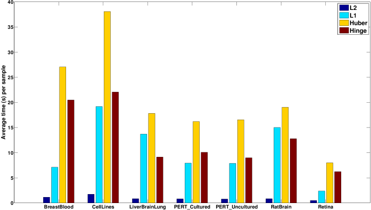
Figure 2: Average computational time for each loss function in different datasets

Computation time, while important, is not the critical measure in our evaluation. The true performance of a configuration (selection of loss function and constraints) is measured by its estimation error. In order to rank different configurations, we first assess the agreement among different measures. To this end, we evaluate each dataset as follows: for each experiment, we compute $\mathbf{mAD,RMSD}$, and $\mathbf{R^{2}D}$ independently. Then, we use Kendall rank correlation, a non-parametric hypothesis test for statistical dependence between two random variables, between each pair of measures and compute a log-transformed p-value for each correlation. Figure 3 shows the agreement among these measures across different datasets. Overall, $RMSD$ and $mAD$ measures show higher consistency, compared to $R^{2}D$ measure. However, the $mAD$ measure is easier to interpret as a measure of percentage loss for each configuration. Consequently, we choose this measure for our evaluation in this study.

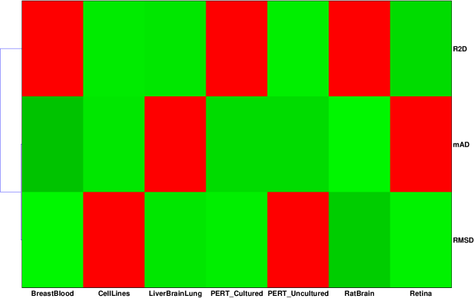
Figure 3: Agreement among different evaluation measures across different datasets

Using $mAD$ as the measure of performance, we evaluate each configuration over each dataset and sort the results. Figure 4 shows various combinations for each dataset. The RatBrain, LiverBrainLung, BreastBlood, and CellLines datasets achieve high performance. Among these datasets, RatBrain, LiverBrainLung, and BreastBlood had the $\boldsymbol{\mathcal{L}}_{2}$ loss function as the best configuration, with the CellLines dataset being less sensitive to the choice of the loss function. Another surprising observation is that for the majority of configurations, enforcing the sum-to-one constraint worsens the results. We investigate this issue in greater depth in Section 3.5.

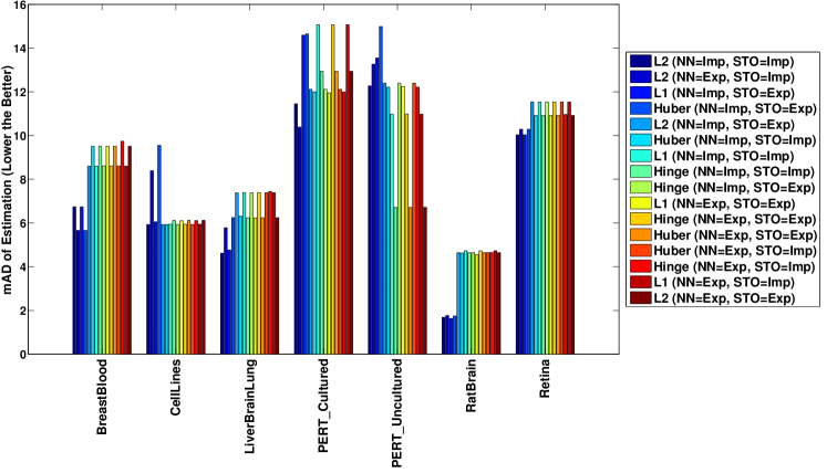
Figure 4: Overall performance of different loss/constraints combinations over all datasets

For Retina, as well as both PERT datasets, the overall performance is worse than the other datasets. In the case of PERT, this is expected, since the flow-sorted proportions are used as an estimate of cell-type proportions. Furthermore, the reference profiles come from a different study and therefore have greater difference with the true cell-types in the mixture. However, the Retina dataset exhibits unusually low performance, which may be attributed to multiple factors. As an initial investigation, we performed a quality control (QC) over different samples to see if errors are similarly distributed across samples. Figure 5 presents per-sample error, measured by $mAD$, with median and median absolute deviation (MAD) marked accordingly. Interestingly, for the $4^{th},6^{th}$, and $8^{th}$ mixtures, the third replicate has much higher error than the rest. In the expression matrix, we observed a lower correlation between these replicates and the other two replicates in the batch. Additionally, for the $7^{th}$ mixture, all three replicates show high error rates. We expand on these results in later sections to identify additional reasons that contribute to the low deconvolution performance of the Retina dataset.

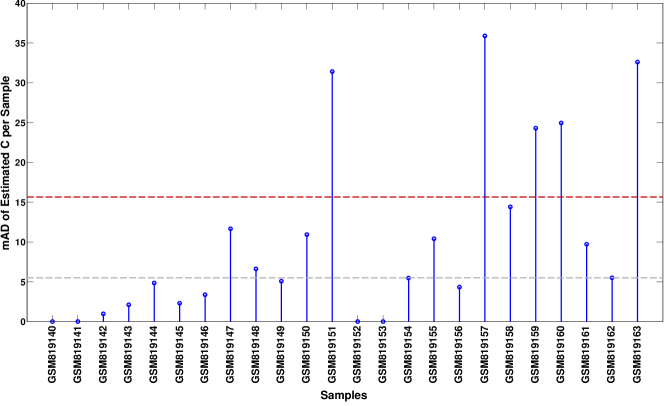
Figure 5: Sample-based error of the Retina dataset, based on $\boldsymbol{\mathcal{L}}_{2}$ with explicit NN and STO

Finally, we note that in all test cases the performance of $\boldsymbol{\mathcal{L}}_{1},\boldsymbol{\mathcal{L}}_{Huber}$, and $\boldsymbol{\mathcal{L}}_{Hinge}$ are comparable, while $\boldsymbol{\mathcal{L}}_{Huber}$ and $\boldsymbol{\mathcal{L}}_{Hinge}$ needed an additional step of parameter tuning. Consequently, we only consider $\boldsymbol{\mathcal{L}}_{1}$ as a representative of this “robust” group of loss functions in the rest of our study.

3.5 Agreement of Gene Expressions with Sum-to-One (STO) Constraint

Considering the lower performance of configurations that explicitly enforce STO constraints, we aim to investigate whether features (genes) in each dataset respect this constraint. Under the STO and NN constraints, we use simple bounds for identifying violating features, for which there is no combination of concentration values that can satisfy both STO and NN. Let $\boldsymbol{m}(i)$ be the expression value of the $i^{th}$ gene in the given mixture, and $\mathbf{G}(i,1),\cdots,\mathbf{G}(i,q)$ be the corresponding expressions in different reference cell-types. Let $\mathbf{G}_{min}(i)=\textbf{min}\{\mathbf{G}(i,1),\cdots,\mathbf{G}(i,q)\}$ and $\mathbf{G}_{max}(i)=\textbf{max}\{\mathbf{G}(i,1),\cdots,\mathbf{G}(i,q)\}$. Given that all concentrations are bound between $0\leq\boldsymbol{c}(k)\leq 1;\forall 1\leq k\leq k$, the minimum and maximum values that an estimated mixture value for the $i^{th}$ gene can attain are $\mathbf{G}_{min}(i)$ and $\mathbf{G}_{max}(i)$, respectively (by setting $\boldsymbol{c}(k)=1$ for min/max value, and $0$ everywhere else). Using this notation, we can identify features that violate STO as follows:

$$\boldsymbol{m}(i)\leq\mathbf{G}_{min}(i)\quad \forall 1\leq i\leq n\quad$$ {Violating reference}

$$\mathbf{G}_{max}(i)\leq\boldsymbol{m}(i)\quad \forall 1\leq i\leq n\quad$$ {Violating mixture}

The first condition holds because expression values in reference profiles are so large that we need the sum of concentrations to be lower than one to be able to match the corresponding gene expression in the mixture. The second condition holds in cases where the expression of a gene in the mixture is so high that we need the sum of concentrations to be greater than one to be able to match it. In other words, for feature $i$, these constraints identify extreme expression values in reference profiles and mixture samples, respectively. Using these conditions, we compute the total number of features violating STO condition in each dataset.

Figure 6 presents violating features in mixtures and reference profiles, averaged over all mixture samples in each dataset. We normalize and report the percent of features to account for differences in the total number of features in each dataset. We first observe that for the majority of datasets, except Retina and BreastBlood, the percent of violating features is much smaller than violating features in reference profiles. These two datasets also have the highest number of violating features in their reference profiles, summing to a total of approximately $60\%$ of all features. This observation is likely due to the normalization used in pre-processing microarray profiles. Specifically, one must not only normalize $\mathbf{M}$ and $\mathbf{G}$ independently, but also with respect to each other. We suggest using control genes that are expressed in all cell-types with low variation to normalize expression profiles. A recent study aimed to identify subsets of housekeeping genes in human tissues that respect these conditions [41]. Another choice is using ribosomal proteins, the basic building blocks of the cellular translation machinery, which are expressed in a wide range of species. The Remove Unwanted Variation (RUV) [42] method is developed to remove batch effects from microarray and RNASeq expression profiles, but also to normalize them using control genes. A simple extension of this method can be adopted to solve the normalization difference between mixtures and references.

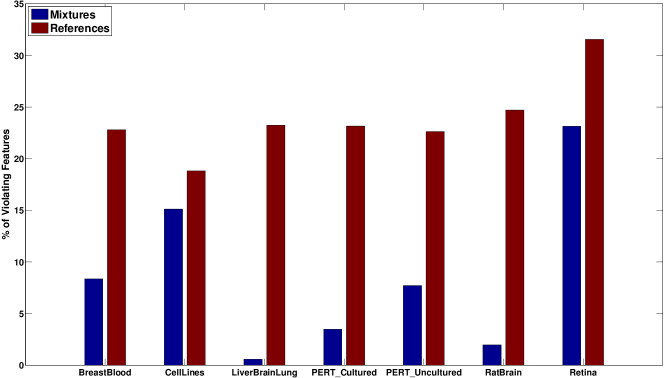
Figure 6: Percent of features in each dataset that violate the STO constraint

Next, we evaluate how filtering these features affects deconvolution performance of each dataset. For each case, we run deconvolution using all configurations and report the change (delta mAD) independently. Figure 7 presents changes in the $mAD$ estimation error after removing violating features in both $\boldsymbol{m}$ and $\mathbf{G}$ before performing deconvolution. Similar to previous experiments, the Retina dataset exhibits widely different behavior than the rest of the datasets. Removing this dataset from further consideration, we find that the overall performance over all datasets improves, with the exception of the RatBrain dataset. In the case of the RatBrain dataset, we hypothesize that the initially superior performance can be attributed to highly expressed features. These outliers, that happens to agree with the true solution, result in over-fitting. Finally, we note a correlation between observed enhancements and the level of violation of features in $\boldsymbol{m}$. Consistent with this observation, we obtain similar results when we only filter violating features from mixtures, but not reference profiles.

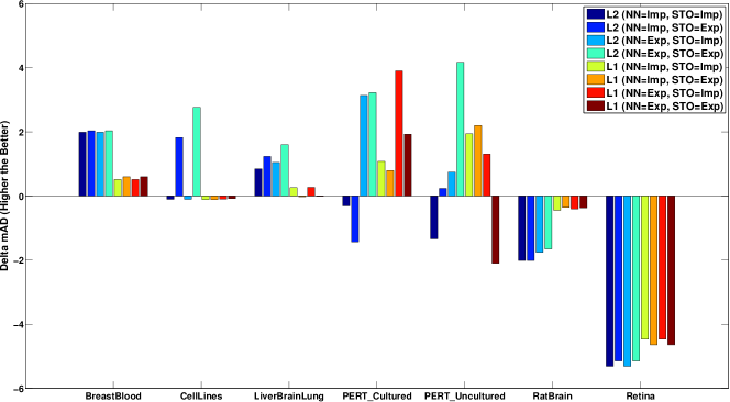
Figure 7: Performance of deconvolution methods after removing violating features

3.6 Range Filtering– Finding an Optimal Threshold

Different upper/lower bounds have been proposed in the literature to prefilter expression values prior to deconvolution. For example, Gong et al. [22] suggest an effective range of $[0.5,5000]$, whereas Ahn et al. [43] observe an optimal range of $[2^{4}-2^{14}]$. To facilitate the choice of expression bounds, we seek a systematic way to identify an optimal range for different datasets. Kawaji et al. [44] recently report on an experiment to assess whether gene expression is quantified linearly in mixtures. To this end, they mix two cell-types (THP-1 and HeLa cell-lines) and see if experimentally measured expressions match with the computationally simulated datasets. They observe that expression values for microarray measurements are skewed for the lowly expressed genes (approximately $<10$). This allows us to choose the lower bound based on experimental evidence. In our study, we search for the optimal bounds over a $log_{2}$-linear space; thus, we set a threshold of $2^{3}$ on the minimum expression values, which is closest to the bound proposed by Kawaji et al. [44].

Choosing an upper bound on the expression values is a harder problem, since it relates to enhancing the performance of deconvolution methods by removing outliers. Additionally, there is a known relationship between the mean expression value and its variance [45], which makes these outliers noisier than the rest of the features. This becomes even more important when dealing with purified cell-types that come from different labs, since highly expressed time/micro-environment dependent genes would be significantly different than the ones in the mixture [21]. A simple argument is to filter genes that the range of expression values in Affymetrix microarray technology is bounded by $2^{16}$ (due to initial normalization and image processing steps). Measurements close to this bound are not reliable as they might be saturated and inaccurate. However, practical bounds used in previous studies are far from these extreme values. In order to examine the overall distribution of expression values, we analyze different datasets independently. For each dataset, we separately analyze mixture samples and reference profiles, encoded by matrices $\mathbf{M}$ and $\mathbf{G}$, respectively. For each of these matrices, we vectorize the expression values and perform kernel smoothing using the Gaussian kernel to estimate the probability density function.

Figure 8(a) and Figure 8(b) show the distribution of log-transformed expression values for mixtures and reference profiles, respectively. These expression values are greater than our lower bound of $2^{3}$. In agreement with our previous results, we observe an unusually skewed distribution for the Retina dataset, which in turn contributes to its lower performance compared to other ideal mixtures. Additionally, we observe that approximately $80\%$ of the features in this dataset are smaller than $2^{3}$, which are filtered and not shown in the distribution plot. For the rest of the datasets, in both mixtures and references, we observe a bell-shaped distribution with most of the features captured up to an upper bound of $2^{8}-2^{10}$. Another exception to this pattern is the CellLines dataset, which has a heavier tail than other datasets, especially in its reference profile.

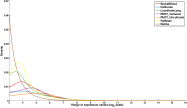
(a) Mixtures

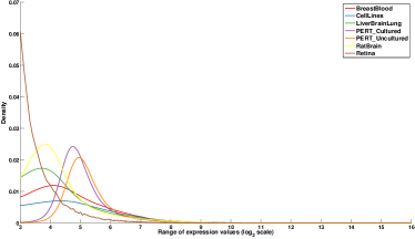
(b) Reference Profiles

Figure 8: Distribution of expression values

Next, we systematically evaluate the effect of range filtering by analyzing upper bounds increasing in factors of 10 in the range $\{2^{5},\cdots,2^{16}\}$. In each case, we remove all features that at least one of the reference profiles or mixture samples has a value exceeding this upper bound. Figure 9 illustrates the percent of features that are retained, as we increase the upper bound. As mentioned earlier, approximately $80\%$ of the features in the Retina dataset are lower than $2^{3}$, which is evident from the maximum percent of features left to be bounded by $20\%$ in this figure. Additionally, consistent with our previous observation over expression densities, more that $80\%$ of the features are covered between $2^{8}-2^{10}$, except for the CellLine dataset.

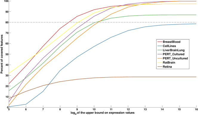
Figure 9: Percent of covered features during range filtering

Finally, we perform deconvolution using the remaining features given each upper bound. The results are mixed, but a common trend is that removing highly expressed genes decreases performance of ideal mixtures with known concentrations, while enhancing the performance of PERT datasets. Figure 10(a) and Figure 10(b) show the changes in mAD error, compared to unfiltered deconvolution, for the PERT dataset. In each case, we observe improvements up to 7 and 8 percent, respectively. The red and green points on the diagram show the significance of deconvolution. Interestingly, while both methods show similar improvements, all data points for cultured PERT seem to be insignificant, whereas uncultured PERT shows significance for the majority of data-points. This is due to the weakness of our random model, which is dependent on the number of samples and is not comparable across datasets. Uncultured PERT has twice as many samples as cultured PERT, which makes it less likely to have any random samples achieving as good an mAD as the observed estimation error. This dependency on the number of samples can be addressed by defining sample-based p-values. Another observation is that for the uncultured dataset, all measures have been improved, except $\boldsymbol{\mathcal{L}}_{1}$ with explicit NN and STO constraints. On the other hand, for the cultured dataset, both $\boldsymbol{\mathcal{L}}_{1}$ and $\boldsymbol{\mathcal{L}}_{2}$ with the explicit NN constraint perform well, whereas implicitly enforcing NN deteriorates their performance. Cultured and uncultured datasets have their peak at $2^{10}$ and $2^{12}$, respectively.

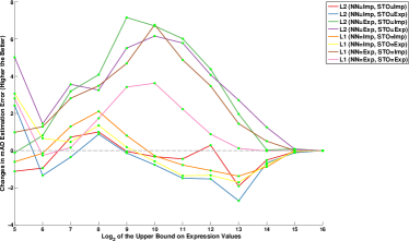
(a) Cultured

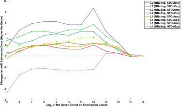
(b) Uncultured

Figure 10: Performance of PERT datasets during range filtering

For the rest of the datasets, range filtering decreased performance in a majority of cases, except the Retina dataset, which had an improved performance at $2^{6}$ with the best result achieved with $\boldsymbol{\mathcal{L}}_{1}$ with both explicit NN and STO enforcement. This changed the best observed performance of this datasest, measured as mAD, to be close to 7. These mixed results make it harder to choose a threshold for the upper bound, so we average results over all datasets to find a balance between improvements in PERT and overall deterioration in other datasets. Figure 11 presents the averaged mAD difference across all datasets. This suggests a “general” upper bound filter of $2^{12}$ to be optimal across all datasets.

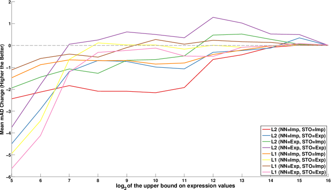
Figure 11: Average performance of range filtering over all datasets

We use this threshold to filter all datasets and perform deconvolution on them. Figure 12 presents the dataset-specific performance of range filtering with fixed bounds, measured by changes in the mAD value compared to the original deconvolution. As observed from individual performance plots, range filtering is most effective in cases where the reference profiles differ significantly from the true cell-types in the mixture, such as the case with the PERT datasets. In ideal mixtures, since cell-types are measured and mixed at the same time/laboratory, this distinction is negligible. In these cases, highly expressed genes in mixtures and references coincide with each other and provide additional clues for the regression. Consequently, removing these highly expressed genes often degrades the performance of deconvolution methods. This generalization of the upper bound threshold, however, should be adopted with care, since each dataset exhibits different behavior in response to range filtering. Ideally, one must filter each dataset individually based on the distribution of expression values. Furthermore, in practical applications, gold standards are not available to aid in the choice of cutoff threshold.

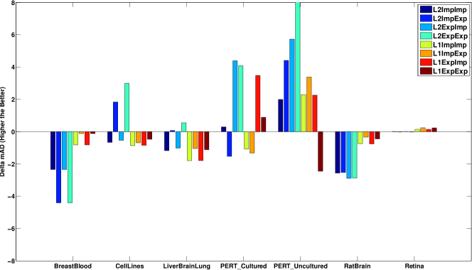
Figure 12: Dataset-specific changes in the performance of deconvolution methods after filtering expression ranges to fit within $[2^{3}-2^{12}]$

We now introduce a new method that adaptively identifies an effective range for each dataset. Figure 13 illustrates the $log_{2}$ normalized value of maximal expression for each gene in matrices $\mathbf{M}$ and $\mathbf{G}$, sorted in ascending order. In all cases, intermediate values exhibit a gradual increase, whereas the top and bottom elements in the sorted list show a steep change in their expression. We aim to identify the critical points corresponding to these sudden changes in the expression values for each dataset. To this end, we select the middle point as a point of reference and analyze the upper and lower half, independently. For each half, we find the point on the curve that has the longest distance from the line connecting the first (last) element to the middle element. Application of this process over the CellTypes dataset is visualized in Figure 14. Green points in this figure correspond to the critical points, which are used to define the lower and upper bound for the expression values of this dataset.

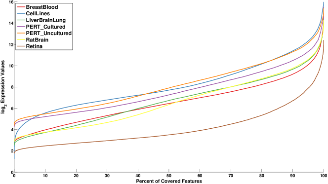
Figure 13: Sorted $log_{2}$-transformed gene expressions in different datasets

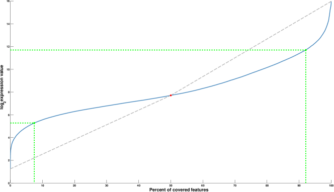
Figure 14: Example of adaptive filtering over CellLines dataset

We use this technique to identify adaptive ranges for each dataset prior to deconvolution. Table II summarizes the identified critical points for each dataset. Figure 15 presents the dataset-specific performance of each method after adaptive range filtering. While in most cases the results for fixed and adaptive range filtering are compatible, and in some cases adaptive filtering gives better results, the most notable difference is the degraded performance of LiverBrainLung, and, to some extent, RatBrain datasets. To further investigate this observation, we examine individual experiments for these datasets for fixed thresholds. Figure 16 illustrates individual plots for each dataset. The common trend here is that in both cases range filtering, in general, degrades the performance of deconvolution methods for all configurations. In other words, extreme values in these datasets are actually helpful in guiding the regression, and any filtering negatively impacts performance. This suggests that range filtering, in general, is not always helpful in enhancing the deconvolution performance, and in fact in some cases; for example the ideal datasets such as LiverBrainLung, RatBrain, and BreastBlood; it can be counterproductive.

TABLE II: Summary of adaptive ranges for each dataset

	LowerBound	UpperBound
BreastBlood	4.2842	9.4314
CellLines	5.2814	11.6942
LiverBrainLung	3.3245	9.9324
PERT_Cultured	4.9416	10.9224
PERT_Uncultured	5.1674	11.5042
RatBrain	3.3726	9.9698
Retina	2.4063	6.7499

Figure 15: Dataset-specific changes in the performance of deconvolution methods after adaptive range filtering

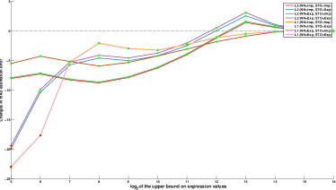
(a) LiverBrainLung

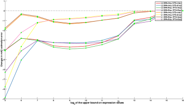
(b) RatBrain

Figure 16: Individual performance plots for range filtering in datasets which range filtering exhibits negative effect on the deconvolution

3.7 Selection of Marker Genes – The Good, Bad, and Ugly

Selecting marker genes that uniquely identify a certain tissue or cell-type, prior to deconvolution, can help in improving the conditioning of matrix $\mathbf{G}$, thus improving its discriminating power and stability of results, as well as decreasing the overall computation time. A key challenge in identifying “marker” genes is the choice of method that is used to assess selectivity of genes. Various parametric and nonparametric methods have been proposed in literature to identify differentially expressed genes between two groups [46, 47] or between a group and other groups [48]. Furthermore, different methods have been developed in parallel to identify tissue-specific and tissue-selective genes that are unique markers with high specificity to their host tissue/cell type [49, 50, 51, 52]. While choosing/developing accurate methods for identifying reliable markers is an important challenge, an in-depth discussion of the matter is beyond the scope of this article. Instead, we adopt two methods used in the literature. Abbas et al. [20] present a framework for choosing genes based on their overall differential expression. For each gene, they use a t-test to compare the cell-type with the highest expression with the second and third highest expressing cell-type. Then, they sort all genes and construct a sequence of basis matrices with increasing sizes. Finally, they use condition number to identify an “optimal” cut among top-ranked genes that minimizes the condition number. Newman et al. [15] propose a modification to the method of Abbas et al., in which genes are not sorted based on their overall differential expression, but according to their tissue-specific expression when compared to all other cell-types. After prefiltering differentially expressed genes, they sort genes based on their expression fold ratio and use a similar cutoff that optimizes the condition number. Note that the former method increases the size of the basis matrix by one at each step, while the latter method increases it by $q$ (number of cell-types). The method of Newman et al. has the benefit that it chooses a similar number of markers per cell-type, which is useful in cases where one of the references has a significantly higher number of markers.

We implement both methods and assess their performance over the datasets. We observe slightly better performance with the second method and use it for the rest of our experiments. Due to unexpected behavior of the Retina dataset, as well as a low number of significant markers in all our trials, we eliminate this dataset from further study. In identifying differentially expressed genes, a key parameter is the q-value cutoff to report significant features. The distribution of corrected p-values exhibits high similarity among ideal mixtures, while differing significantly in CellLines mixtures and both PERT datasets. We find the range of $10^{-3}-10^{-5}$ to be an optimal balance between these two cases and perform experiments to test different cutoff values. Figure 17 shows changes in the $mAD$ measure after applying marker detection, using a q-value cutoff of $10^{-3}$, which resulted in the best overall performance in our study. We observe that the PERT_Uncultured and LiverBrainLung datasets have the highest gain across the majority of configurations, while BreastBlood and RatBrain exhibit an improvement in experiments with $\boldsymbol{\mathcal{L}}_{1}$ while their $\boldsymbol{\mathcal{L}}_{2}$ performance is greatly decreased. Finally, for the PERT_Cultured and CellLines datasets, we observe an overall decrease in performance in almost all configurations.

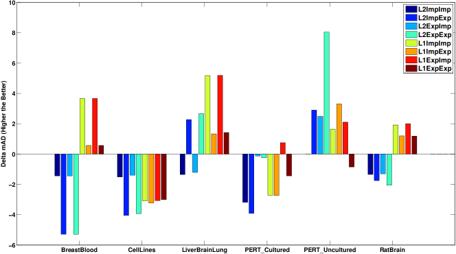
Figure 17: Effect of marker selection on the performance of deconvolution methods

Next, we note that the internal sorting based on fold-ratio intrinsically prioritizes highly expressed genes and is susceptible to noisy outliers. To test this hypothesis, we perform a range selection using a global upper bound of $10^{12}$ prior to the marker selection method and examine if this combination can enhance our previous results. We find the q-value threshold of $10^{-5}$ to be the better choice in this case. Figure 18 shows changes in performance of different methods when we prefilter expression ranges prior to marker selection. The most notable change is that both the PERT_Cultured and the CellLines, which were among the datasets with the lowest performance in the previous experiment, are now among the best-performing datasets, in terms of overall mAD enhancement. We still observe a higher negative impact on $\boldsymbol{\mathcal{L}}_{2}$ in this case, but the overall amplitude of the effect has been dampened in both BreastBlood and RatBrain datasets.

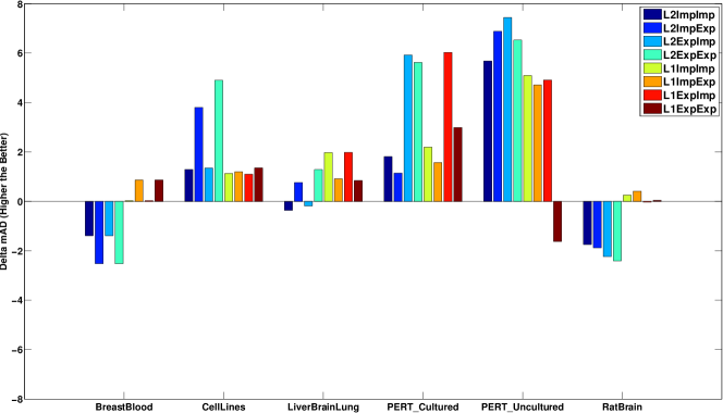
Figure 18: Effect of marker selection, after range filtering, on the performance of deconvolution methods

We note that there is no prior knowledge as to the “proper” choice of the marker selection method in the literature and that their effect on the deconvolution performance is unclear. An in-depth comparison of marker detection methods can benefit future developments in this field. An ideal marker should serve two purpose: (i) be highly informative of the cell-type in which it is expressed, (ii) shows low variance due to spatiotemporal changes in the environment (changes in time or microenvironment). Figure 19 shows a high-level classification of genes. An ideal marker is an invariant, cell-type specific gene, marked with green in the diagram. On the other hand, variant genes, both universally expressed and tissue-specific, are not good candidates, especially in cases where references are adopted from a different study. These genes, however, comprise ideal subsets of genes that should be updated in full deconvolution while updating matrix $\mathbf{G}$, since their expression in the reference profile may differ significantly from the true cell-types in the mixture. It is worth mentioning that the proper ordering to identify best markers is to first identify tissue-specific genes and then prune them based on their variability. Otherwise, when selecting invariant genes, we may select many housekeeping genes, since their expression is known to be more uniform compared to tissue-specific genes.

Another observation relates to the case in which groups of profiles of cell-types have high similarity within the group, but are significantly distant from the rest. This makes identifying marker genes more challenging for these groups of cell-types. An instance of this problem is when we consider markers in the PERT datasets. In this case, erythrocytes have a much larger number of distinguishing markers compared to other references. This phenomenon is primarily attributed to the underlying similarity between undifferentiated cell-types in the PERT datasets, and their distance from the fully differentiated red blood cells. In these cases, it is beneficial to summarize each group of similar tissues using a “representative profile” for the whole group, and to use a hierarchical structure to recursively identify markers at different levels of resolution [52].

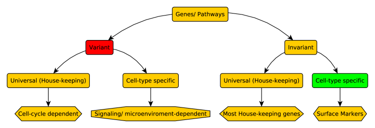
Figure 19: High-level classification of genes

Finally, we examine the common choice of condition number as the optimal choice to select the number of markers. First, unlike the “U” shape plot reported in previous studies, in which condition number initially decreases to an optimal point and then starts increasing, we observe variable behavior in the condition number plot, both for Newman et al. and Abbas et al. methods. This makes the generalization of condition number as a measure applicable to all datasets infeasible. Additionally, we note that the lowest condition number is achieved if $\mathbf{G}$ is fully orthogonal, that is $\mathbf{G}^{T}\mathbf{G}=\kappa\mathbf{I}$ for any constant $\kappa$. By selecting tissue-selective markers, we can ensure that the product of columns in the resulting matrix is close to zero. However, the norm-2 of each column can still be different. We developed a method that specifically grows the basis matrix by accounting for the norm equality across columns. We find that in all cases our basis matrix has a lower condition number than both the Newman et al. and Abbas et al. methods, but it did not always improve the overall performance of deconvolution methods using different loss functions. Further study on the optimal choice of the number of markers is another key question that needs further investigation

3.8 To Regularize or Not to Regularize

We now evaluate the impact of regularization on the performance of different deconvolution methods. To isolate the effect of the regularizer from prior filtering/feature selection steps, we apply regularization on the original datasets. The $\boldsymbol{\mathcal{R}}_{1}$ regularizer is typically applied in cases where the solution space is large, that is, the total number of available reference cell-types is a superset of the true cell-types in the mixture. This type of regularization acts as a “selector” to choose the most relevant cell-types and zero-out the coefficients for the rest of the cell-types. This has the effect of enforcing a sparsity pattern. Datasets used in this study are all controlled benchmarks in which references are hand-picked to match the ones in the mixture; thus, sparsifying the solution does not add value to the deconvolution process. On the other hand, an $\boldsymbol{\mathcal{R}}_{2}$ regularizer, also known as Tikhonov regularization, is most commonly used when the problem is ill-posed. This is the case, for example, when the underlying cell-types are highly correlated with each other, which introduces dependency among columns of the basis matrix. In order to quantify the impact of this type of regularization on the performance of deconvolution methods, we perform an experiment similar to the one in Section 3.4 with an added $\boldsymbol{\mathcal{R}}_{2}$ regularizer. In this experiment, we use $\boldsymbol{\mathcal{L}}_{1}$ and $\boldsymbol{\mathcal{L}}_{2}$ loss functions, as we previously showed that the performance of the other two loss functions is similar to $\boldsymbol{\mathcal{L}}_{1}$. Instead of using Ridge regression introduced in Section 2.4.2, we implement an equivalent formulation, $\parallel\boldsymbol{m}-\mathbf{G}\boldsymbol{c}\parallel_{2}+\lambda\parallel\boldsymbol{c}\parallel_{1}$, which traces the same path but has higher numerical accuracy. To identify the optimal value of the $\lambda$ parameter that balances the relative importance of solution fit versus regularization, we search over the range of $\{10^{-7},\cdots,10^{7}\}$. It is notable here that when $\lambda$ is close to zero, the solution is identical to the one without regularization, whereas when $\lambda\rightarrow\infty$ the deconvolution process is only guided by the solution size. Similar to the range filtering step in Section 3.6, we use the minimum mAD error to choose the optimal value of $\lambda$.

Figure 20 presents changes in mAD error, compared to original errors, after regularizing loss functions with the $\boldsymbol{\mathcal{R}}_{2}$ regularizer. From these observations, it appears that PERT_Cultured has the most gain due to regularization, whereas for PERT_Uncultured, the changes are smaller. A detailed investigation, however, suggests that in the majority of cases for PERT_Cultured, the performance gain is due to over shrinkage of vector $\boldsymbol{c}$ to the case of being almost uniform. Interestingly, the choice of uniform $\boldsymbol{c}$ has lower mAD error for this dataset compared to most other results. Overall, both of the PERT datasets show significant improvements compared to the original solution, which can be attributed to the underlying similarity among hematopoietic cells. On the other hand, an unexpected observation is the performance gain over $\boldsymbol{\mathcal{L}}_{1}$ configurations for the BreastBlood dataset. This is primarily explained by the limited number of cell-types (only two), combined with the similar concentrations used in all samples (only combinations of $67\%$ and $33\%$).

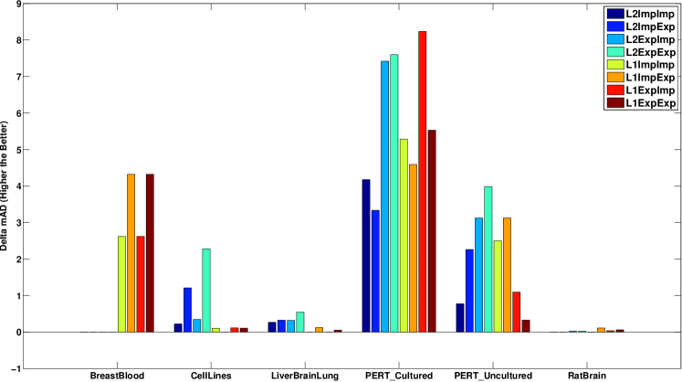
Figure 20: Effect of L2 regularization on the performance of deconvolution methods

To gain additional insight into the parameters used in each case during deconvolution, we plot the optimal $\lambda$ values for each configuration in each dataset. Figure 21 summarizes the optimal values of the $\lambda$ parameter. Large values indicate a beneficial effect for regularization, whereas small values are suggestive of negative impact. In all cases where the overall mAD score has been improved, their corresponding $\lambda$ parameter was large. However, large values of $\lambda$ do not necessarily indicate a significant impact on the final solution, as is evident in the CellLines and LiverBrainLung datasets. Finally, we observe that cases where the value of $\lambda$ is close to zero are primarily associated with the $\boldsymbol{\mathcal{L}}_{2}$ loss function.

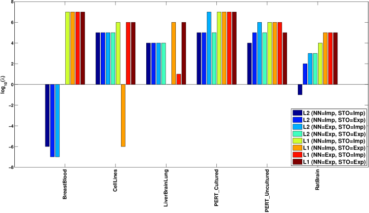
Figure 21: Optimal value of $\lambda$ for each dataset/configuration pair

3.9 Summary

Based on our observations, we propose the following guidelines for the deconvolution of expression datasets:

1. Pre-process reference profiles and mixtures using invariant, universally expressed (housekeeping) genes to ensure that the similar cell quantity (SCQ) constraint is satisfied.

2. Filter violating features that cannot satisfy the sum-to-one (STO) constraint.

3. Filter lower and upper bounds of gene expressions using adaptive range filtering.

4. Select invariant (among references and between references and samples) cell-type-specific markers to enhance the discriminating power of the basis matrix.

5. Solve the regression using the $\boldsymbol{\mathcal{L}}_{1}$ loss function with explicit constraints (check), together with an $\boldsymbol{\mathcal{R}}_{2}$ regularizer, or group LASSO if sparsity is desired among groups of tissues/cell-types.

6. Use the L-curve method to identify the optimal balance between the regression fit and the regularization penalty.

4 Concluding Remarks

In this paper, we present a comprehensive review of different methods for deconvolving linear mixtures of cell-types in complex tissues. We perform a systematic analysis of the impact of different algorithmic choices on the performance of the deconvolution methods, including the choice of the loss function, constraints on solutions, data filtering, feature selection, and regularization. We find $\boldsymbol{\mathcal{L}}_{2}$ loss to be superior in cases where the reference cell-types are representative of constitutive cell-types in the mixture, while $\boldsymbol{\mathcal{L}}_{1}$ outperforms the $\boldsymbol{\mathcal{L}}_{2}$ in cases where this condition does not hold. Explicit enforcement of the sum-to-one (STO) constraint typically degrades the performance of deconvolution. We propose simple bounds to identify features violating this constraint and evaluate the total number of violating features in each dataset. We observe an unexpectedly high number of features that cannot satisfy the STO condition, which can be attributed to problems with normalization of expression profiles, specifically normalizing references and samples with respect to each other. In terms of filtering the range of expression values, we find that fixed thresholding is not effective and develop an adaptive method for filtering each dataset individually. Furthermore, we observed that range filtering is not always beneficial for deconvolution and, in fact, in some cases it can deteriorate the performance. We implement two commonly used marker selection methods from the literature to assess their effect on the deconvolution process. Orthogonalizing reference profiles can enhance the discriminating power of the basis matrix. However, due to known correlation between the mean and variance of expression values, this process alone does not always provide satisfactory results. Another key factor to consider is the low biological variance of genes in order to enhance the reproducibility of the results and allow deconvolution with noisy references. The combination of range filtering and marker selection eliminates genes with high mean expression, which in turn enhances the observed results. Finally, we address the application of Tikhonov regularization in cases where reference cell-types are highly correlated and the regression problem is ill-posed.

We summarize our findings in a simple set of guidelines and identify open problems that need further investigation. Areas of particular interest for future research include: (i) identifying the proper set of filters based on the datasets, (ii) expanding deconvolution problem to cases with more complex, hierarchical structure among reference vectors, and (iii) selecting optimal features to reduce computation time while maximizing the discriminating power.

Shahin Mohammadi received his Master’s degree in Computer Science from Purdue University in Dec. 2012 and is currently a Ph.D. candidate at Purdue. His research interests include computational biology, machine learning, and parallel computing. His current work spans different areas of Bioinformatics/Systems Biology and aims to develop computational methods coupled with statistical models for data-intensive problems, with application in mining the human tissue-specific transcriptome and interactome.

Neta Zuckerman received her PhD degree in computational biology from the University of Bar-Ilan, Israel in June 2010. She has completed her post-doctorate in 2015 as a computational biologist at Stanford University, School of Medicine and City of Hope as well as a visiting scholar at the department of Electrical Engineering, Stanford University. Her research interests focus on investigating the role of immune cells in the setting of various diseases, specifically cancer, utilizing algorithm development and microarray data analysis. Neta is currently a computational biologist at Genentech Inc.

Andrea Goldsmith Andrea Goldsmith is the Stephen Harris professor in the School of Engineering and a professor of Electrical Engineering at Stanford University. Her research interests are in information theory and communication theory, and their application to wireless communications as well as biology and neuroscience. She has received several awards for her work including the IEEE ComSoc Edwin H. Armstrong Achievement Award, the IEEE ComSoc and Information Theory Society Joint Paper Award, and the National Academy of Engineering Gilbreth Lecture Award. She is author of 3 textbooks, including Wireless Communications, all published by Cambridge University Press, as well as an inventor on 28 patents.

Ananth Grama received the PhD degree from the University of Minnesota in 1996. He is currently a Professor of Computer Sciences and Associate Director of the Center for Science of Information at Purdue University. His research interests span areas of parallel and distributed computing architectures, algorithms, and applications. On these topics, he has authored several papers and texts. He is a member of the American Association for Advancement of Sciences.

References

- [1] Nicolas Gillis “Successive Nonnegative Projection Algorithm for Robust Nonnegative Blind Source Separation” In SIAM Journal on Imaging Sciences 7.2, 2014, pp. 1420–1450 DOI: 10.1137/130946782
- [2] Wing-Kin Ma et al. “A Signal Processing Perspective on Hyperspectral Unmixing: Insights from Remote Sensing” In IEEE Signal Processing Magazine 31.1, 2014, pp. 67–81 DOI: 10.1109/MSP.2013.2279731
- [3] D. Nuzillard and A. Bijaoui “Blind source separation and analysis of multispectral astronomical images” In Astronomy& astrophysics supplement series 147, 2000, pp. 129–138 DOI: 10.1051/aas:2000292
- [4] V. Paul Pauca, J. Piper and Robert J. Plemmons “Nonnegative matrix factorization for spectral data analysis” In Linear Algebra and its Applications 416.1, 2006, pp. 29–47 DOI: 10.1016/j.laa.2005.06.025
- [5] E. Villeneuve and H. Carfantan “Hyperspectral data deconvolution for galaxy kinematics with MCMC” In Signal Processing Conference (EUSIPCO), 2012 Proceedings of the 20th European, 2012, pp. 2477–2481
- [6] Akaysha C Tang, Barak A Pearlmutter, Michael Zibulevsky and Scott A Carter “Blind source separation of multichannel neuromagnetic responses” In Neurocomputing 32–33, 2000, pp. 1115 –1120 DOI: http://dx.doi.org/10.1016/S0925-2312(00)00286-1
- [7] C.W. Hesse and C.J. James “On Semi-Blind Source Separation Using Spatial Constraints With Applications in EEG Analysis” In Biomedical Engineering, IEEE Transactions on 53.12, 2006, pp. 2525–2534 DOI: 10.1109/TBME.2006.883796
- [8] Carlos Vaya, José J. Rieta, César Sanchez and David Moratal “Convolutive blind source separation algorithms applied to the electrocardiogram of atrial fibrillation: Study of performance” In IEEE Transactions on Biomedical Engineering 54.8, 2007, pp. 1530–1533 DOI: 10.1109/TBME.2006.889778
- [9] Kun Zhang and Aapo Hyvärinen “Source Separation and Higher-Order Causal Analysis of MEG and EEG” In CoRR abs/1203.3533, 2012 URL: http://arxiv.org/abs/1203.3533
- [10] M.S. Pedersen, U. Kjems, K.B. Rasmussen and L.K. Hansen “Semi-blind source separation using head-related transfer functions [speech signal separation]” In Acoustics, Speech, and Signal Processing, 2004. Proceedings. (ICASSP ’04). IEEE International Conference on 5, 2004, pp. V–713–16 vol.5 DOI: 10.1109/ICASSP.2004.1327210
- [11] Meng Yu, Wenye Ma, Jack Xin and Stanley Osher “Multi-Channel l1 Regularized Convex Speech Enhancement Model and Fast Computation by the Split Bregman Method” In Audio, Speech, and Language Processing, IEEE Transactions on 20.2 IEEE, 2012, pp. 661–675
- [12] Emmanuel Vincent, Nancy Bertin, Rémi Gribonval and Frédéric Bimbot “From blind to guided audio source separation: How models and side information can improve the separation of sound” In IEEE Signal Processing Magazine 31.3 Institute of Electrical and Electronics Engineers (IEEE), 2014, pp. 107–115 URL: https://hal.inria.fr/hal-00922378
- [13] Nathan Souviraà-Labastie, Anaik Olivero, Emmanuel Vincent and Frédéric Bimbot “Multi-channel audio source separation using multiple deformed references” In IEEE Transactions on Audio, Speech and Language Processing 23.11 Institute of Electrical and Electronics Engineers (IEEE), 2015, pp. 1775–1787 URL: https://hal.inria.fr/hal-01070298
- [14] Alexandre Kuhn et al. “Cell population-specific expression analysis of human cerebellum.” In BMC genomics 13, 2012, pp. 610 DOI: 10.1186/1471-2164-13-610
- [15] Aaron M Newman et al. “Robust enumeration of cell subsets from tissue expression profiles” In Nature Methods, 2015, pp. 1–10 DOI: 10.1038/nmeth.3337
- [16] Shai S Shen-Orr and Renaud Gaujoux “Computational deconvolution: extracting cell type-specific information from heterogeneous samples.” In Current opinion in immunology 25.5, 2013, pp. 571–8 DOI: 10.1016/j.coi.2013.09.015
- [17] Olvi L. Mangasarian and David R. Musicant “Robust Linear and Support Vector Regression” In IEEE Trans. Pattern Anal. Mach. Intell. 22.9, 2000, pp. 950–955 DOI: 10.1109/34.877518
- [18] Vladimir Vapnik “Statistical learning theory” Wiley, 1998
- [19] Alex J. Smola and Bernhard Schölkopf “A Tutorial on Support Vector Regression” In Statistics and Computing 14.3 Hingham, MA, USA: Kluwer Academic Publishers, 2004, pp. 199–222 DOI: 10.1023/B:STCO.0000035301.49549.88
- [20] Alexander R Abbas et al. “Deconvolution of blood microarray data identifies cellular activation patterns in systemic lupus erythematosus.” In PloS one 4.7, 2009, pp. e6098 DOI: 10.1371/journal.pone.0006098
- [21] Wenlian Qiao et al. “PERT: a method for expression deconvolution of human blood samples from varied microenvironmental and developmental conditions.” In PLoS computational biology 8.12, 2012, pp. e1002838 DOI: 10.1371/journal.pcbi.1002838
- [22] Ting Gong et al. “Optimal deconvolution of transcriptional profiling data using quadratic programming with application to complex clinical blood samples.” In PloS one 6.11, 2011, pp. e27156 DOI: 10.1371/journal.pone.0027156
- [23] Z. Altboum et al. “Digital cell quantification identifies global immune cell dynamics during influenza infection” In Molecular Systems Biology 10.2, 2014, pp. 720–720 DOI: 10.1002/msb.134947
- [24] Shai S Shen-Orr et al. “Cell type-specific gene expression differences in complex tissues.” In Nature methods 7.4, 2010, pp. 287–9 DOI: 10.1038/nmeth.1439
- [25] Jingu Kim, Yunlong He and Haesun Park “Algorithms for nonnegative matrix and tensor factorizations: a unified view based on block coordinate descent framework” In Journal of Global Optimization 58.2, 2013, pp. 285–319 DOI: 10.1007/s10898-013-0035-4
- [26] D. Venet, F. Pecasse, C. Maenhaut and H. Bersini “Separation of samples into their constituents using gene expression data” In Bioinformatics 17.Suppl 1, 2001, pp. S279–S287 DOI: 10.1093/bioinformatics/17.suppl“˙1.S279
- [27] Dirk Repsilber et al. “Biomarker discovery in heterogeneous tissue samples -taking the in-silico deconfounding approach.” In BMC bioinformatics 11, 2010, pp. 27 DOI: 10.1186/1471-2105-11-27
- [28] Neta S Zuckerman, Yair Noam, Andrea J Goldsmith and Peter P Lee “A self-directed method for cell-type identification and separation of gene expression microarrays.” In PLoS computational biology 9.8, 2013, pp. e1003189 DOI: 10.1371/journal.pcbi.1003189
- [29] Renaud Gaujoux and Cathal Seoighe “Semi-supervised Nonnegative Matrix Factorization for gene expression deconvolution: a case study.” In Infection, genetics and evolution : journal of molecular epidemiology and evolutionary genetics in infectious diseases 12.5, 2012, pp. 913–21 DOI: 10.1016/j.meegid.2011.08.014
- [30] Yi Zhong et al. “Digital sorting of complex tissues for cell type-specific gene expression profiles.” In BMC bioinformatics 14, 2013, pp. 89 DOI: 10.1186/1471-2105-14-89
- [31] Timo Erkkilä et al. “Probabilistic analysis of gene expression measurements from heterogeneous tissues.” In Bioinformatics (Oxford, England) 26.20, 2010, pp. 2571–7 DOI: 10.1093/bioinformatics/btq406
- [32] Wenjun Ju et al. “Defining cell-type specificity at the transcriptional level in human disease.” In Genome research 23.11, 2013, pp. 1862–73 DOI: 10.1101/gr.155697.113
- [33] Gerald Quon et al. “Computational purification of individual tumor gene expression profiles leads to significant improvements in prognostic prediction.” In Genome medicine 5.3, 2013, pp. 29 DOI: 10.1186/gm433
- [34] David A Liebner, Kun Huang and Jeffrey D Parvin “MMAD: microarray microdissection with analysis of differences is a computational tool for deconvoluting cell type-specific contributions from tissue samples.” In Bioinformatics (Oxford, England) 30.5, 2014, pp. 682–9 DOI: 10.1093/bioinformatics/btt566
- [35] Renaud Gaujoux and Cathal Seoighe “CellMix: a comprehensive toolbox for gene expression deconvolution.” In Bioinformatics (Oxford, England) 29.17, 2013, pp. 2211–2 DOI: 10.1093/bioinformatics/btt351
- [36] Alexandre Kuhn et al. “Population-specific expression analysis (PSEA) reveals molecular changes in diseased brain.” In Nature methods 8.11, 2011, pp. 945–7 DOI: 10.1038/nmeth.1710
- [37] Sandra Siegert et al. “Transcriptional code and disease map for adult retinal cell types” In Nature Neuroscience 15.3, 2012, pp. 487–495 DOI: 10.1038/nn.3032
- [38] Michael Grant and Stephen Boyd “Graph implementations for nonsmooth convex programs” http://stanford.edu/~boyd/graph_dcp.html In Recent Advances in Learning and Control, Lecture Notes in Control and Information Sciences Springer-Verlag Limited, 2008, pp. 95–110
- [39] “CVX: Matlab Software for Disciplined Convex Programming, version 2.1”, http://cvxr.com/cvx, 2014
- [40] “The MOSEK optimization software” URL: http://www.mosek.com/
- [41] Eli Eisenberg and Erez Y. Levanon “Human housekeeping genes, revisited” In Trends in Genetics 29.10, 2013, pp. 569–574 DOI: 10.1016/j.tig.2013.05.010
- [42] Johann A Gagnon-Bartsch and Terence P Speed “Using control genes to correct for unwanted variation in microarray data.” In Biostatistics (Oxford, England) 13.3, 2012, pp. 539–52 DOI: 10.1093/biostatistics/kxr034
- [43] Jaeil Ahn et al. “DeMix: deconvolution for mixed cancer transcriptomes using raw measured data.” In Bioinformatics (Oxford, England) 29.15, 2013, pp. 1865–71 DOI: 10.1093/bioinformatics/btt301
- [44] H. Kawaji et al. “Comparison of CAGE and RNA-seq transcriptome profiling using clonally amplified and single-molecule next-generation sequencing” In Genome Research 24.4, 2014, pp. 708–717 DOI: 10.1101/gr.156232.113
- [45] Y Tu, G Stolovitzky and U Klein “Quantitative noise analysis for gene expression microarray experiments.” In Proceedings of the National Academy of Sciences of the United States of America 99.22, 2002, pp. 14031–14036 DOI: 10.1073/pnas.222164199
- [46] Marine Jeanmougin et al. “Should we abandon the t-test in the analysis of gene expression microarray data: a comparison of variance modeling strategies.” In PloS one 5.9, 2010, pp. e12336 DOI: 10.1371/journal.pone.0012336
- [47] Neil R Clark et al. “The characteristic direction: a geometrical approach to identify differentially expressed genes” In BMC Bioinformatics 15.1, 2014, pp. 79 DOI: 10.1186/1471-2105-15-79
- [48] K Van Deun et al. “Testing the hypothesis of tissue selectivity: the intersection-union test and a Bayesian approach.” In Bioinformatics (Oxford, England) 25.19, 2009, pp. 2588–94 DOI: 10.1093/bioinformatics/btp439
- [49] Florence M G Cavalli et al. “SpeCond: a method to detect condition-specific gene expression.” In Genome biology 12.10, 2011, pp. R101 DOI: 10.1186/gb-2011-12-10-r101
- [50] Koji Kadota et al. “ROKU: a novel method for identification of tissue-specific genes.” In BMC bioinformatics 7, 2006, pp. 294 DOI: 10.1186/1471-2105-7-294
- [51] Kenneth D Birnbaum and Edo Kussell “Measuring cell identity in noisy biological systems.” In Nucleic acids research 39.21, 2011, pp. 9093–107 DOI: 10.1093/nar/gkr591
- [52] Shahin Mohammadi and Ananth Grama “A novel method to enhance the sensitivity of marker detection using a refined hierarchical prior of tissue similarities”, 2015 DOI: 10.1101/020685