Abstract

Abstract. We consider the problem of matching two shapes assuming these shapes are related by an elastic deformation. Using linearized elasticity theory and the finite element method we seek an elastic deformation that is caused by simple external boundary forces and accounts for the difference between the two shapes. Our main contribution is in proposing a cost function and an optimization procedure to minimize the symmetric difference between the deformed and the target shapes as an alternative to point matches that guide the matching in other techniques. We show how to approximate the nonlinear optimization problem by a sequence of convex problems. We demonstrate the utility of our method in experiments and compare it to an ICP-like matching algorithm.

1 Introduction

1.1 Motivation

Understanding two-dimensional shape and its variations is one of the fundamental problems in computer vision, computer graphics, and medical imaging. In particular, finding correspondences between two given input shapes is the basis of many applications such as recognition and information transfer. One way for finding correspondences between shapes is to compute a deformation that aligns one shape (the source) with the other (the target). This problem is usually referred to as the shape matching problem.

From a mathematical stand point the shape matching problem is an ill-posed inverse problem. This is because a desired matching is often tied with the unknown semantics of the given shapes. The usual way to cope with this is though regularization, i.e., one balances the quality of a correspondence against its regularity.

1.2 Our Method

In this work we propose an alternative shape matching algorithm in two dimensions to ICP and ICP-like methods. In addition we will provide a comparison to our ICP-like methods, recently introduced in [48, 49]. Our approach minimizes the area of mutual non-overlap, i.e., the area of the symmetric difference of the compared shapes. This is a global dissimilarity measure and a low value, in contrast to ICP, assures a good (but not necessarily meaningful) alignment of the deformable source and the fixed target shape.

To find meaningful alignments we use linearized elasticity as a regularizer for the deformation. More specifically, we seek to explain deformations of the source shape by means of elastic forces acting on the shape boundary. This is a reasonable strategy since many shapes in applications depict actual physical bodies and hence shape change can be explained by means of external causes. We furthermore believe that in many scenarios an observed deformation can be explained by very simple causes, i.e., the physical forces that cause the shape change are simple although the deformation itself may not be simple. The reader may think of articulations of a given object, such as a human shape or a moving animal, where forces mostly act on the articulated parts. This motivates to look for boundary forces that are sparse while simultaneously seeking a good alignment. This is in the spirit of [46], as one usually seeks a good alignment by means of minimal cost.

The optimization problem we pose is nonlinear. We show a heuristic way to approximate the problem by a sequence of (convex) second order cone problems (SOCPs). Our shapes are represented by their outlines which we use to build triangular meshes of them. The finite element method (FEM) then allows us to discretize the underlying equations of linearized elasticity, the Navier-Lamé equations, and to derive a linear relation between (nodal) boundary displacements and (nodal) boundary forces. This is done by a reduction of the stiffness matrix and yields a suitable representation of the elastic regularizer that only involves the boundary.

The area of the symmetric difference is computed by first finding its polygonal outline and then computing the area by means of the divergence theorem. The polygon describing the symmetric difference is computed using Vatti’s clipping algorithm [52], which was originally used in the context of rendering. Note that the triangular mesh is only needed for the initial step of the FEM, i.e., the computation of the stiffness matrix. The optimization, though, takes place on the boundary (of the mesh) only, which reduces the number of variables while keeping information of the elastic properties of the interior of the source shape.

1.3 Related Work

Overview.

An optimization based shape matching algorithm is, as already insinuated, usually based on the principle of seeking a good alignment while keeping a deformation cost, measured on an admissible set of deformations, as low as possible.

Rigid matching, i.e., the admissible deformations are translations and rotations, is considered to be well-understood [1, 26, 43]. These low-dimensional deformations are the first choice when it comes to the alignment of range scans of rigid objects.

In the case of non-rigid matching there is a larger variety of deformation models. The authors of [8, 21], for instance, model a deformable medium as a fluid that gradually deforms into the desired target. This was done in the context of medical image matching and has the advantage that it allows very large deformations. Elastic regularizers, on the other hand, are in clear contrast to fluid regularizers as they do carry information about previous deformation states (fluids do not have “memory”). They have been pioneered in computer graphics by Terzopoulos [51] and in medical imaging by Broit and Bajcsy [7, 25]. In particular, in the context of matching, elasticity based (or related) methods have been used in [5, 7, 24, 42]. Overviews can be found in [28, 40].

Both, fluid and elasticity methods model shape as a continuum and hence contain information of the behavior of their interior. Shapes can also be outlined by their contours such as polygonal lines. Matching then amounts to curve matching and is usually a lower dimensional problem due to the compact curve representation. Younes [53, 54] models curves by their associated angle functions and a group action on this representation models deformation. An energy modeling elastic behavior of the curve is then minimized to obtain correspondences. The authors of [37] model a Riemannian structure on a manifold of curves and match them by finding geodesics on this manifold. The geodesic distance is then used as a comparison measure between shapes. Note that modeling shapes as curve outlines does not a priori take into account their interior. A good survey on curve matching can be found in [55].

Measuring the alignment of the shapes is the second ingredient for an optimization based algorithm. A well-known method is the so-called iterative closest point algorithm introduced by Besl and McKay [10]. ICP is an iterative method that aligns shapes by altering between finding a good transform and updating nearest neighbor correspondences. This amounts to minimizing mean distance of the shapes by means of nearest neighbor correspondences. It has been used originally for rigid matching. Refined variants based on different correspondence rejection and weighting methods can be found in [43]. For more recent non-rigid variants of ICP see [2, 17, 31]. Our methods introduced in [48, 49] are modifications of classical ICP since we allow estimated correspondences to drift during the optimization instead of keeping them fixed. Therefore, we refer to them as ICP-like methods.

The nearest neighbor distance used in ICP can be seen as the $L^{2}$-version of the one-sided Hausdorff distance [23]. It is not symmetric and hence not a metric. In contrast, the area of symmetric difference constitutes a metric on the space of shapes. Minimizing a dissimilarity metric for matching is called metric matching. A theoretical result for matching convex shapes measured by the symmetric difference can be found in [3]. There the authors show that aligning the centroids of the shapes guarantees that their symmetric difference is within a certain bound of the optimum. Unfortunately this only holds for a rather restrictive set of transforms and shapes. More practically oriented approaches can be found in the context of segmentation and registration using level set methods [47], see [18, 19, 41]. There, the shapes are represented as level set functions, and functionals derived from the Chan-Vese model [18, 19] are minimized. The area/volume of the symmetric difference was also used for finding a shape median [9] and in the context of elastic shape averaging [44]. These approaches are (also) closely related to minimizing the Mumford-Shah functional [38]. In [9] a Chan-Vese model is employed and in [44] shapes are encoded by means of a so-called phase field function [4].

Other metric dissimilarity measures in the literature, used for metric matching, include the Hausdorff distance [29], the Gromov-Hausdorff distance [15, 35] and the Gromov-Wasserstein distance[35, 36]. These metrics are either rather hard to compute or can suffer from robustness issues.

Comparison.

The work presented in this paper borrows methods from linearized elasticity to measure the difficulty of shape change. The splitting of the stiffness matrix that we employ to minimize boundary forces was previously used in the context of surgery simulations [13] and in our approach to two-dimensional shape matching in [48]. In contrast to minimizing the elastic energy or to computing geodesic lengths, which is done in most of the above cited works that employ elasticity, seeking unknown forces has the advantage that we get an explanation of the unknown deformation in addition to the deformation itself. In particular sparse forces, we believe, can account for simple explanations. This principle was generalized in [49] in the ICP-like setting to nonlinear elastic matching in three dimensions.

Both of our previous ICP-like schemes employ (descriptor aided) nearest neighbor correspondences to drive the search for an alignment. The difference to our symmetric difference method is that for the latter we do not use any kind of “guessed” correspondences or other shape information like curvature or descriptors. This renders the method simple. Both methods have in common that the estimated correspondences and the negative gradient of the area of the symmetric difference, which we use in the optimization, can be interpreted as a restoring force between source and target that needs to be regularized. Furthermore, our previous methods and our symmetric difference method can be classified as local methods since they converge to a local minimum that depends on the initial alignment of the shapes.

We provide experimental evidence that our method can outperform the ICP-like method [48] in two dimensions by means of robustness and alignment. Indeed, the ICP-like method is not guaranteed to give a good alignment since it can theoretically converge to a single point on the target shape. In contrast, a low area of the symmetric difference always means a good (and by means of regularization hopefully meaningful) overlap.

Our symmetric difference method relates to methods used for metric matching [9, 18, 19, 41, 44] but uses completely different tools. All the above cited literature represent shapes using a level set approach and make use of their indicator functions. This amounts to an area based method. For the computation of the symmetric difference and its area we, in contrast, solely make use of its polygonal outline. For this an efficient version of Vatti’s algorithm for polygonal clipping is the essential ingredient. Since we also reduce the elastic regularizer to the boundary of the source shape this essentially amounts to matching closed curves. Note that on the other hand we keep elastic information of the interior of the shape and can compute interior displacements by simply solving a linear system of equations. This way we take advantage of the lower dimension of the optimization problem on the boundary while not losing information of the interior of the shape.

This work is organized as follows. In Section 2 we give an overview of the relevant part of elasticity theory and of the properties of the area of symmetric difference. We also give a detailed explanation of the optimization problem that we solve in a heuristic manner. Section 4 gives an overview of the implementation and shows results of experiments with shapes taken from various data sets. A direct comparison to our method introduced in [48] is provided. Section 5 concludes with a discussion.

2 Methods

2.1 Linearlized Elasticity and FEM

We give a concise overview of the parts of linearized elasticity and the finite element framework that are relevant to this work. Additional and more detailed material about elasticity theory can be found in [20, 22]. For more material on FEM see [12, 22].

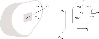
Figure 1: Left: an illustration of a surface force $t(x,n)$ at some point $x$ in an arbitrary cross section with normal $n$ of a body $B$. Right: illustration of the three components of the stress tensor with respect to the canonical coordinate planes. The normal stress is orthogonal to the considered plane shear stresses lie within the plane.

We begin by explaining linearized elasticity theory in 3D. Elasticity theory explains the states of elastic bodies that are subject to external forces. An elastic body is a physical entity, described by a closed connected and bounded set $\mathcal{B}\subset\mathbb{R}^{3}$, that reacts to external forces with a deformation and returns to its original shape after the forces are removed. An elastic body has no memory of previous deformations or applied forces.

The elasticity equations describe the balance between external forces $g$, applied to a an elastic body, and internal forces that resist the deformation caused by the external ones. The basic equation reads

$$\begin{split}-\operatorname{div}\sigma&=g\quad\text{in $\mathcal{B}$}\>,\\ \end{split}$$ (1)

where $\sigma$ is called the Cauchy stress tensor (or simply stress), represented by a $3$-by-$3$-matrix. Roughly speaking, $\sigma$ measures the internal stress distribution, i.e., for any $x\in\mathcal{B}$ it yields the resulting surface traction $t(x,n)$ (force measured per unit area) among all cross-sections given by their surface unit normal $n$. The stress is symmetric and material specific. An illustration of the traction is given in Figure 1.

The material specific reaction of a body to applied forces in linearized elasticity is modeled by a linear relation between strain and stress. Strain measures the local change of lengths inside a solid body. It is rotation invariant and can hence not be linear. In linearized elasticity we use its first order approximation which is given by $\varepsilon=1/2(\nabla u+\nabla u^{T})$ where $u:\mathcal{B}\rightarrow\mathbb{R}^{3}$ is the displacement field, i.e., $x\in\mathcal{B}$ moves to $\Phi(x)=x+u(x)$. $\Phi$ is the so-called deformation field. The strain measure $\varepsilon$ is not invariant under general Euclidean motions but only under translations and infinitesimal rotations. The linear relation between stress and strain is usually encoded in a fourth-order tensor but assuming homogeneity and isotropy of the solid it can be simplified to Hooke’s law:

$$\sigma=\lambda\operatorname{tr}(\varepsilon)\mathbb{I}+2\mu\varepsilon\>.$$ (2)

The constants $\lambda$ and $\mu$ are the Lamé constants, $\operatorname{tr}(\cdot)$ is the trace and $\mathbb{I}$ denotes the identity. This model is often used in engineering since it approximates the elastic behavior of solids very well provided the deformation is small.

Combining the expressions for $\varepsilon$ and Hookes’s law with (1) we get the Navier-Lamé equation

$$\mu\Delta u+(\lambda+\mu)\nabla\operatorname{div}u+g=0\quad\text{in $\mathcal{B}$}$$ (3)

supplemented with the boundary conditions

$$\begin{split}u&=u_{0}\quad\text{on $\Gamma_{D}$,}\\ \sigma(u)n&=f\quad\;\>\text{on $\Gamma_{N}$}\\ \end{split}$$ (4)

where $\Gamma_{D}$ and $\Gamma_{N}$ are disjoint portions of the boundary $\partial\mathcal{B}$, $n$ is the outward unit normal on $\Gamma_{N}$, and $f$ is a known external surface force. This PDE constitutes a linear elliptic system and is well-posed [12] (up to translation and infinitesimal rotation if $\Gamma_{D}=\emptyset$). For our case of planar shape matching we simply set the third component of the displacement field to zero, i.e., we set $u=(u_{1},u_{2},0)$. This leaves the structure of (3) unchanged.

For a numerical solution of equation (3) on general domains we use a piece-wise continuous finite elements on a triangular mesh. Conformal finite elements rely on the weak form of the underlying PDE which is given in our case as: find $u$ that satisfies the boundary conditions (4) on $\Gamma_{D}$ such that

$$\begin{split}\int_{\mathcal{B}}&\mu\left\langle\nabla u,\nabla v\right\rangle+(\lambda+\mu)(\operatorname{div}u)(\operatorname{div}v)\>\mathrm{d}x\\ &=\int_{\Gamma_{N}}\left\langle f,v\right\rangle\>\mathrm{d}S-\int_{\mathcal{B}}\left\langle g,v\right\rangle\>\mathrm{d}x\quad\forall v\in V\end{split}$$ (5)

where $V$ is a space of suitable test functions. For details see [12, 22]. Conformal FEMs replace $V$ with a finite dimensional approximation $V^{h}$. Choosing a basis in $V^{h}$ one can transform (5) into a linear system of equations for the nodal displacements $u^{h}$

$$Au^{h}=f^{h}-g^{h}\>.$$ (6)

Note, that the traction boundary conditions enter the right-hand side. The system matrix $A$ is called stiffness matrix and is symmetric positive semi-definite. Its rank in case of planar elasticity is $2N-3$ where $N$ is the number of nodes in the mesh and its kernel consists of translations and infinitesimal rotations.

2.2 Properties of the Symmetric Difference

As a comparison measure between shapes the symmetric difference has a few attractive properties. Most importantly, it constitutes a metric on the shape space. This can easily be seen as follows: the symmetric difference as an operation on the power set $\mathcal{P}(X)$ of any given set $X$ makes it an Abelian group with the empty set as the neutral element. Any set $A\in\mathcal{P}(X)$ is inverse to itself. The map $A\mapsto\chi_{A}$, where the right-hand side denotes the indicator function of $A$, defines a group homomorphism from $\mathcal{P}(X)$ into the group of indicator functions endowed with the binary relation $\chi_{A}\bigtriangleup\chi_{B}:=\left\lvert\chi_{A}-\chi_{B}\right\rvert$. Restricting this homomorphism to the set of measurable functions one can express the Lebesgue measure of the symmetric difference as

$$\mu(A\bigtriangleup B)=\int_{\mathbb{R}^{d}}\left\lvert\chi_{A}-\chi_{B}\right\rvert\>\mathrm{d}x=\int_{\mathbb{R}_{d}}\chi_{A\bigtriangleup B}\>\mathrm{d}x\>.$$ (7)

This way it is easy to see that the measure of the symmetric difference fulfills the triangle inequality

$$\mu(A\bigtriangleup B)\leq\mu(A\bigtriangleup C)+\mu(C\bigtriangleup B)$$ (8)

and hence $\mu(\cdot\bigtriangleup\cdot)$ is a pseudo-metric on the set of measurable functions. Identifying all sets that are equal almost everywhere we even get a metric.

Suppose that we are given a pair of semantically similar shapes $\mathcal{S}$ (source) and $\mathcal{T}$ (target). The goal is to find a meaningful transformation $\Phi:\mathcal{S}\rightarrow\mathcal{T}$, i.e., a smooth and locally injective vector field. The admissible shapes are outlined by closed non-self-intersecting curves in two dimensions or orientable manifolds without boundary. Both define a proper area or volume and they can be regarded as the boundaries of solids. We denote with $\mathcal{B}$ the solid represented by $\mathcal{S}$. In particular we have $\partial\mathcal{B}=\mathcal{S}$. $\Phi:\mathcal{B}\rightarrow\mathbb{R}^{3}$ denotes the volumetric deformation of $\mathcal{B}$.

3 The Optimization Problem

3.1 Minimizing the Area of the Symmetric Difference

This paper focuses on the case of planar matching and further assumes zero volumetric forces $g=0$ in (3), i.e., the unknown deformation is caused by boundary forces only. The optimization problem to be solved in our framework can now be formulated as

$$\begin{split}\operatorname*{min}_{\Phi}&\quad\int_{\mathcal{S}}\left\|\sigma(u)n\right\|_{2}\>\mathrm{d}S\\ \text{subject to}&\quad\mu(\Phi(\mathcal{S})\bigtriangleup\mathcal{T})=0\\ &\quad\mu\Delta u+(\lambda+\mu)\nabla\operatorname{div}u=0\quad\text{in $\mathcal{B}$}\\ \quad&\quad\Phi=\mathbb{I}+u\>.\end{split}$$ (9)

The expression $\mu(\Phi(\mathcal{S})\bigtriangleup\mathcal{T})$ refers to the area of the symmetric difference that is defined by the interiors of $\Phi(\mathcal{S})$ and $\mathcal{T}$. This optimization problem has a convex objective, but it is nonlinear in $\Phi$ due to the constraints. We propose a way to tackle this problem heuristically and show how to approximate it by a sequence of convex second order cone problems.

A relaxed formulation can be written as

$$\begin{split}\operatorname*{min}_{\Phi}&\quad\int_{\mathcal{S}}\left\|\sigma(u)n\right\|_{2}\>\mathrm{d}S+\alpha\mu(\Phi(\mathcal{S})\bigtriangleup\mathcal{T})^{2}\\ \text{subject to}&\quad\mu\Delta u+(\lambda+\mu)\nabla\operatorname{div}u=0\quad\text{in $\mathcal{B}$}\\ \quad&\quad\Phi=\mathbb{I}+u\>.\end{split}$$ (10)

After FEM discretization the PDE constraint becomes a linear system of equations (6). Renumbering the nodes one can assume the structure

$$\left(\begin{array}[]{cc}A_{BB}&A_{BI}\\ A_{IB}&A_{II}\\ \end{array}\right)\left(\begin{array}[]{c}u_{B}\\ u_{I}\\ \end{array}\right)=\left(\begin{array}[]{c}f_{B}\\ 0\\ \end{array}\right)\>,$$ (11)

where $u_{B}$ and $f_{B}$ are respectively the vectors of the nodal displacements and forces at the $K$ boundary nodes and $u_{I}$ denotes the displacements at $N-K$ inner nodes. Note that $f_{I}=0$ on the right-hand side of (11) since we assumed only boundary forces. We assume the displacements $u_{i}\in\mathbb{R}^{2}$ and the forces $f_{i}\in\mathbb{R}^{2}$ at each boundary node in $u_{B}\in\mathbb{R}^{2K}$ and $f_{B}\in\mathbb{R}^{2K}$ to be arranged in the following manner:

$$u_{B}=\left(\begin{array}[]{c}u_{1}^{(1)}\\ u_{1}^{(2)}\\ \vdots\\ u_{K}^{(1)}\\ u_{K}^{(2)}\\ \end{array}\right)\hskip 5.69046pt\text{and}\hskip 5.69046ptf_{B}=\left(\begin{array}[]{c}f_{1}^{(1)}\\ f_{1}^{(2)}\\ \vdots\\ f_{K}^{(1)}\\ f_{K}^{(2)}\\ \end{array}\right)$$ (12)

where $u_{i}^{(j)}$ and $f_{i}^{(j)}$ denote the $j$-th component of the displacement (force resp.) at boundary node $i$. By taking the Schur complement with respect to the boundary block $A_{BB}$ we get the relation

$$Su_{B}=f_{B}$$ (13)

where

$$S=A_{BB}-A_{BI}A_{II}^{-1}A_{IB}\>.$$ (14)

We thus completely eliminated the linear system as a constraint and reduced the problem to the boundary curve $\mathcal{S}=\partial\mathcal{B}^{h}$ only. This idea was previously used in [13, 48]. The elastic regularizer is hence reduced to the boundary while keeping information of the elastic properties of the interior. The interior displacements can be found by solving a linear system. In the discretized setting the boundaries $\mathcal{S}$ and $\mathcal{T}$ are simply polygonal lines. Taken together, the optimization problem takes the form

$$\begin{split}\operatorname*{min}_{u^{h}}\quad&\sum_{i=1}^{K}\left\|S_{i}u_{B}\right\|_{2}\>\mathrm{d}S\\ &\quad+\alpha\mu((\mathcal{S}+u^{h}(\mathcal{S}))\bigtriangleup\mathcal{T})^{2}\>.\end{split}$$ (15)

The first term of the objective (15) is already in a convenient form but the second one is nonlinear in $u^{h}$ which represents the interpolated nodal boundary displacements $u_{B}$ acting on $\mathcal{S}$. We replace the second term in the objective by its first-order approximation around a given displacement field $u_{0}^{h}$ on the boundary of $\mathcal{S}$:

$$\begin{split}\operatorname*{min}_{u^{h}}\quad&\sum_{i=1}^{K}\left\|S_{i}u_{B}\right\|_{2}\>\mathrm{d}S\\ &+\alpha\left[\mu((\mathcal{S}+u_{0}^{h}(\mathcal{S}))\bigtriangleup\mathcal{T})\right.\\ &+\left.\nabla\mu((\mathcal{S}+u_{0}^{h}(\mathcal{S}))\bigtriangleup\mathcal{T})(u^{h}-u_{0}^{h})\right]^{2}.\end{split}$$ (16)

This is similar to replacing the $L^{2}$-difference $\left\|I_{1}\circ(\mathbb{I}+u)-I_{2}\right\|^{2}$ of two images $I_{1},I_{2}$ that are to be registered by a transform $\Phi=\mathbb{I}+u$ by its first-order approximation around $u=0$. This was done in [24] in the context of unimodal medical imaging. We further explain how we compute the symmetric difference in Section 3.2.

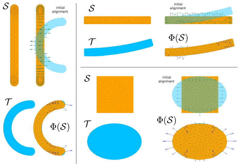
Figure 2: We match three simple source shapes $\mathcal{S}$ to target shapes $\mathcal{T}$. For each experiment we show, in addition, the initial alignment of the shapes together with the negative gradient of the area of the symmetric difference (green arrows) as well as an overlap of the matched shape $\Phi(\mathcal{S})$ and the target together with the elastic forces (blue arrows). The beam-to-C experiment (left) and the ellipse-to-rectangle experiment (lower right) require relatively large deformations.

1

input : Shapes $\mathcal{S},\mathcal{T}$, tolerance $\varepsilon$, elasticity parameters.

2

output : Deformation field $\Phi=\mathbb{I}+u$, deformed meshes $\Phi(\mathcal{B}^{h})$ and boundary forces $f_{B}$.

3

4begin

5      

6      Build a triangulation $\mathcal{B}^{h}$ from the shape outline $\mathcal{S}$;

7      

8      Compute the stiffness matrix of the linear material. Then compute the linear relation between boundary displacements and boundary forces according to (13);

9      

10      Initialize $k=0$ and $u_{k}^{h}=0$;

11      

12      Choose $\alpha$ and $\beta$ initially;

13      

14      while $k\leq K_{\text{max}}$ and $\mu((\mathcal{S}+u_{k}^{h}(\mathcal{S}))\bigtriangleup\mathcal{T})>\varepsilon$ do

15            

16            Compute the measure of the symmetric difference $\mu((\mathcal{S}+u_{k}^{h}(\mathcal{S}))\bigtriangleup\mathcal{T})$ and its gradient at $u_{k}^{h}$ according to Section 3.2;

17            

18            Find the optimal displacement field $u_{k+1}^{h}$ that solves problem (17) (with $u_{0}^{h}=u_{k}^{h}$);

19            

20            Increase $\alpha\leftarrow q\alpha$ and $\beta\leftarrow q\beta$ by a pre-selected constant $q\approx 1.2$ to $1.4$;

21            

22            Set $k\leftarrow k+1$;

23            

24       end while

25      

26      Compute the full deformation of the source shape $\Phi(\mathcal{B}^{h})$ by computing the interior displacements according to (21);

27      

28      Return;

29      

30 end

31

Algorithm 1 Sketch of the symmetric difference algorithm

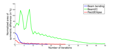
Figure 3: Area of the the symmetric difference in % of the sum of the areas of the source and the target for the experiments shown in Figure 2.

Note that without regularization the minimum of (16) would be zero and the minimizer is not unique and can in principle be a transform with very bad regularity properties. Furthermore, the linear elastic regularizer we use is invariant under translations and infinitesimal rotations. If now any of these transforms is contained in the orthogonal complement of the space spanned by the gradient of $\mu$ at $u_{0}^{h}$, i.e., $\nabla\mu((\mathcal{S}+u_{0}^{h}(\mathcal{S}))\bigtriangleup\mathcal{T})v$ is zero or very small in magnitude, one can still find large displacements that (almost) leave the objective (16) untouched but do significantly increase the area of the symmetric difference. But this is exactly what we want to avoid. Therefore, we add a localization term to (16) to keep the optimal displacement field in average close to $u_{0}^{h}$ which we used as a basis for the linearization. The problem then becomes

$$\begin{split}\operatorname*{min}_{u^{h}}\quad&\sum_{i=1}^{K}\left\|S_{i}u_{B}\right\|_{2}\>\mathrm{d}S+\beta\left\|u^{h}-u_{0}^{h}\right\|_{2}^{2}\\ &+\alpha\left[\mu((\mathcal{S}+u_{0}^{h}(\mathcal{S}))\bigtriangleup\mathcal{T})\right.\\ &+\left.\nabla\mu((\mathcal{S}+u_{0}^{h}(\mathcal{S}))\bigtriangleup\mathcal{T})(u^{h}-u_{0}^{h})\right]^{2}\>.\end{split}$$ (17)

Although we can not guarantee the monotonicity of the functional we observed in experiments that on average we decrease the symmetric difference of the mapped source and the target shape. Note that (17) is a convex problem. We summarized the optimization strategy to solve (9) in Algorithm 1.

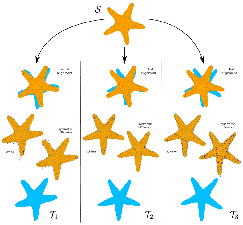
Figure 4: Three articulations of a starfish shape $\mathcal{S}$. We compare the results of the symmetric difference method to the ICP-like method. Visually the results look similar but the ICP-like methods exhibits higher forces and distortion. The elastic forces that produce the matching deformations are shown in blue together with an overlay of the matched shape and the target. Both iterations were stopped once the area of the symmetric difference dropped below $0.7$% of the sum of the area of source and target.

3.2 Computing the Symmetric Difference

Looking at the objective function (17) the reader can see that we need to compute the symmetric difference of two given shapes and its derivative with respect to a variation of one of the shapes.

We start with the area. In order to compute the exact area of the symmetric difference one needs to know the actual symmetric difference of the two shapes or at least their intersection. For shapes bounded by polygonal lines one can find their intersection by means of polygonal clipping algorithms. Clipping algorithms emerged early in computer graphics in the context of rendering. Given a “visible area”, outlined by a closed polygon $P_{1}$, and given another polygon $P_{2}$, the goal

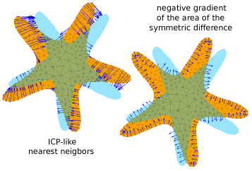
Figure 5: Comparison of the initial restoring forces that are produced by the ICP-like method and the symmetric difference method for target shape $\mathcal{T}_{3}$ in Figure 4.

is to remove the “invisible” part of $P_{2}$ that is outside the visible region of interest, i.e., outside $P_{1}$. The visible area $P_{1}$ is called clip polygon and the polygon $P_{2}$ that is to be clipped is called subject polygon. In other words a clipping algorithm finds a new polygon $P_{3}$ that outlines the area of intersection of the clip and subject polygon.

The basic idea for a convex clip polygon $P_{1}$ is that its interior can be described as the intersection of a finite number of half planes described by its edges. Hence, one can simply throw away the parts of $P_{2}$ that are outside by deciding on which side of the intersection half-planes of $P_{1}$ these parts are. This is the basis for the Sutherland-Hodgman algorithm [50]. For non-convex clip polygons one can still define the inside of a polygonal curve by the winding number as done in the Greiner-Hormann algorithm [27]. However, we use a version of Vatti’s clipping algorithm [52] which is slower in performance but does not suffer from degeneracies as the Greiner-Hormann algorithm.

Now, we are equipped with a tool that finds the outline of the area of the symmetric difference. Computing the measure of this area can then simply be done by means of the divergence theorem, i.e., one needs to compute a (discrete) boundary integral.

The computation of the gradient of $\mu(\mathcal{S}\bigtriangleup\mathcal{T})$ with respect to a variation of $\mathcal{S}$ is equivalent to computing the gradient of $\mu((\mathcal{S}+u^{h}(\mathcal{S}))\bigtriangleup\mathcal{T})$ with respect to a small variation of the displacement field $u^{h}$ on the boundary $\mathcal{S}$. Since $u^{h}$ is finite dimensional the gradient is a vector of length $2K$ where $K$ is the number of boundary nodes as in (17). This is done by means of a finite difference scheme and requires $2K$ applications of the clipping algorithm and $2K$ evaluations of the area.

The number of applications of the clipping algorithm can be reduced to $K$ by the following argument: By means of the divergence theorem we reduced the computation of the area of the symmetric difference to the boundary of $\mathcal{S}$. The gradient flow of the symmetric difference minimization

$$\partial_{t}\mathcal{S}=-\nabla_{\mathcal{S}}\mu(\mathcal{S}\bigtriangleup\mathcal{T})$$ (18)

describes its evolution as a curve. The evolution of any curve along an arbitrary velocity field $v$ is governed only by the contribution of $v$ that points in shape’s normal direction. The tangential part of $v$ just affects the curve parametrization. But reparametrization does not affect the area of the symmetric difference $\mu(\mathcal{S}\bigtriangleup\mathcal{T})$. Since $-\nabla_{\mathcal{S}}\mu(\mathcal{S}\bigtriangleup\mathcal{T})$ is the direction of steepest descent this rules out any contribution in tangential directions. Hence, given the shape normals one can compute the gradient of the symmetric difference by computing its directional derivative in normal direction only. Since estimating shape normals is cheaper than polygon clipping this reduces the computational cost for gradient calculation by roughly $1/2$. This is an application of the Epstein-Gage lemma [30] for curve evolution.

4 Implementation and Experiments

The implementation was done on a standard desktop PC with a modern quad core processor and 8GB of RAM using MATLAB. Looking at (17) the reader can see that there are three major bottleneck routines. First, one needs to compute the matrix $S$ that describes the relation between boundary displacements and boundary forces. For this we use our own implementation in $C$.

The second bottleneck is the efficient computation of the symmetric difference. For this we use, as said before, Vatti’s algorithm. The C-library GPC [39] implements this algorithm and is used in our implementation. For two input polygons (clip and subject) the algorithm generates a clipped polygon that outlines the intersection area of both inputs or the area outlining the result of any other Boolean operation like the set difference or the symmetric difference.

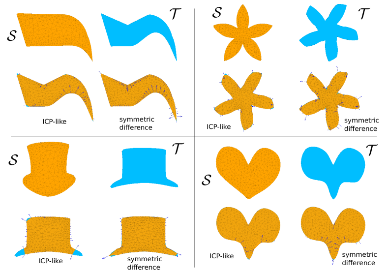
Figure 6: Four examples of matching in which the symmetric difference algorithm outperforms the ICP-like method. The latter produced flipped triangles in all examples as well as a bad alignment in case of the hat experiment (lower left). The elastic forces found by each algorithm are shown in blue together with an overlay of the matched shape and the target.

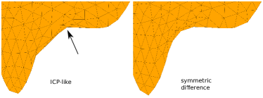
Figure 7: Close-up of the heart experiment shown in Figure 6. The ICP-like method produces flipped triangles in contrast to the symmetric difference method.

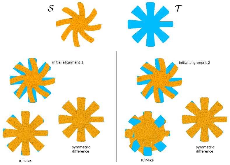
Figure 8: Comparison of the effect of a slight change of the initial alignment of source $\mathcal{S}$ and target $\mathcal{T}$. The symmetric difference method still yields a good match while the ICP-like method fails for the second initial alignment. The initial alignments differ by a rotation of the source of 10 degree around its center of mass.

The third bottleneck is the optimization procedure itself. For this note that problem (17) can be written in the form of a second order cone problem

$$\begin{split}\operatorname*{min}_{f_{i},d,e}&\quad\sum_{i=1}^{K}f_{i}+\alpha d+\beta e\\ \text{subject to}&\quad\left\|S_{i}u_{B}\right\|_{2}\leq f_{i}\>,\quad i=1\dots K\>,\\ &\quad\left\|\left(\begin{array}[]{c}2F(u^{h})\\ d-1\end{array}\right)\right\|_{2}\leq d+1\>,\\ &\quad\left\|\left(\begin{array}[]{c}2(u^{h}-u_{0}^{h})\\ e-1\end{array}\right)\right\|_{2}\leq e+1\\ \end{split}$$ (19)

where

$$\begin{split}F(u^{h})&=\mu((\mathcal{S}+u_{0}^{h}(\mathcal{S}))\bigtriangleup\mathcal{T})\\ &\quad+\nabla\mu((\mathcal{S}+u_{0}^{h}(\mathcal{S}))\bigtriangleup\mathcal{T})(u^{h}-u_{0}^{h})\>.\end{split}$$ (20)

Among many good solvers for this type of problems we found that MOSEK [6] is very efficient and used it through the YALMIP interface [34].

We conducted several experiments in order to show that our algorithm performs well. The example shapes have been taken form [45, 48] and the MPEG-7 dataset [32]. The first step was to extract the (polygonal) boundary curve from the images that contain the shapes as a dense ordered point set. Then we meshed the interior of the shapes to obtain a Delaunay triangulation for the FEM. This is necessary to compute the stiffness matrix of the relevant material. The triangulations contained between 200 to 700 triangles. As Lamé constants we chose $\mu=1$ and $\lambda=0$. This way the material is allowed to stretch without shrinking in the lateral direction [42].

For comparison we use the shape matching algorithm we introduced in [48] as a baseline method. In the sequel we will refer to it as the “ICP-like” algorithm. Recall that this algorithm is similar to ICP except that we allow boundary correspondences to drift during the optimization.

The first experiment, see Figure 2, shows three simple shapes that are matched to each other using our symmetric difference method. In the figure we show, in addition to the shapes, the negative gradient of the area of the symmetric difference in the initial position. This gradient can be interpreted as a restoring or driving force that acts on the boundary of the solid represented by $\mathcal{S}$. Note, that an initial overlap of the source and the target is necessary for this gradient to contain information about the desired final shape. The areas of the symmetric difference in each iteration are shown in Figure 3. One can see that on average the area of symmetric difference decreases towards zero. We stopped the algorithm at most 50 iterations or if the area of the symmetric difference dropped below a certain threshold (1% of the sum of the areas of the source and the target). Also note that the deformations are quite large for a linear material model.

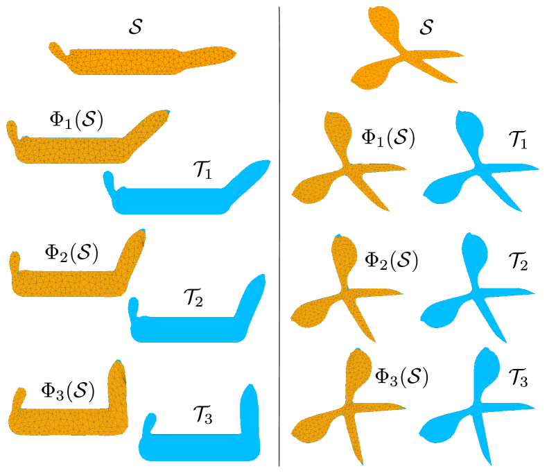
Figure 9: Two examples of gradually increasing deformations taken from the tool dataset described in [14, 16]. The symmetric difference method produces good alignment but can suffer from large distortion and flipped triangles as the deformation becomes very large.

In the second experiment, Figure 4, we match the shape of a starfish to three different articulations. We compare the results of our symmetric difference method to the results that we got by our ICP-like method (using the same initial alignment) in terms of iteration numbers, norm of forces and conformal distortion, see Table 1. Although the results appear to be visually similar the symmetric difference method generally produced smaller elastic forces and conformal distortions (in maximum and average) while slightly more iterations were needed.

	$\mathcal{T}_{1}$	$\mathcal{T}_{2}$	$\mathcal{T}_{3}$
# Iterations
Symmetric difference	19	21	19
ICP-like	14	15	14
Norm of forces
Symmetric difference	0.41	0.82	0.95
ICP-like	0.45	0.92	0.97
Maximal CD
Symmetric difference	2.15	12.46	1.89
ICP-like	4.04	98.1	2.92
Mean CD
Symmetric difference	1.14	1.18	1.18
ICP-like	1.15	1.35	1.24

Table 1: Comparison of the symmetric difference method to the ICP-like method in terms of number of iterations, norm of forces and conformal distortion (CD) in each triangle, see Figure 4.

Figure 5 shows the initial restoring force produced by the symmetric difference method compared to the restoring forces that are initially produced by the ICP-like method. The ICP-like forces are at many places of the boundary unreasonable due to nearest neighbors that are far away from the correct correspondences. The symmetric difference method produces forces that tend to shrink the source $\mathcal{S}$ in regions that do not overlap with the target $\mathcal{T}$ while it tends to expand the shape in regions of overlap.

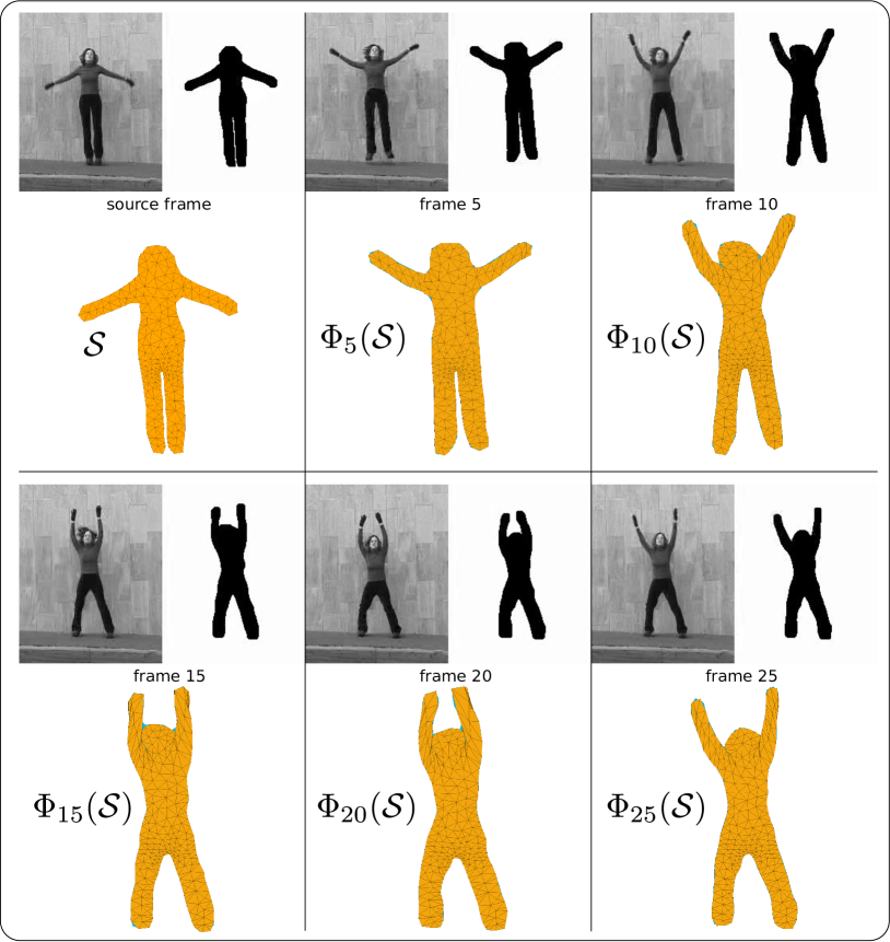
Figure 10: We track the gradually increasing deformation of the silhouette of a jumping person taken from a video sequence that consists of 28 frames. The first frame serves as a source frame. We then match the source to the target silhouette in the $n$-th frame, starting from $n=2$. The resulting deformation was then used to initialize the method for matching the source to the target silhouette of the $(n+1)$-th frame. We show the result for the frame numbers 5, 10, 15, 20, and 25. Note that although the deformation becomes quite large the method yields good alignment but can suffer frome flipped triangles and large conformal distortion.

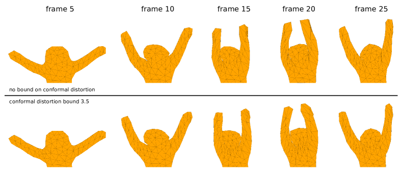
Figure 11: Close up of the experiment shown in Figure 10 without distortion bound (upper row). We compare to it the visual effects of adding a global distortion bound of $3.5$ in the same experiment (lower row). The results in the lower row does not show flipped triangles and it is guaranteed that the maximal conformal distortion does not exceed the bound of $3.5$.

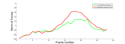
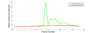
Figure 12: The graphs compare the jumping person experiment shown in Figure 10 to the same experiment with an additional global bound on the conformal distortion. Bounding the distortion leads to slightly higher forces (left) and lower distortion in average (right). The peak of the mean conformal distortion on the right-hand side (green) without distortion bound was reached in the frames when the deformation was most developed. For the red graphs we used a global distortion bound of $3.5$. See also Figure 11 for a visual comparison.

Furthermore, we observed that in many scenarios the symmetric difference method outperforms the ICP-like method. Figure 6 shows four examples in which the ICP-like methods produced not only higher conformal distortion but also resulted in flipped triangles in contrast to the symmetric difference method. A close-up view of one of the experiments is shown in Figure 7.

Both of these methods are local and hence sensitive to initial alignment of source and target. As the shape matching problem is ill-posed the situation is even worse since a slight change of the initial alignment can produce completely different results of the methods. We observed in experiments that the symmetric difference is often less sensitive to a slight change of the initial alignment compared to the ICP-like method which relies on the computation of nearest neighbors. This is demonstrated in Figure 8.

Our method can be used to track gradually increasing deformations. Figure 9 shows two examples taken from the tool dataset [14, 16] and Figure 10 shows the tracking of a gradually increasing deformation taken from a video sequence used in [11]. The video sequence, which depicts a jumping person, contains the presegmented silhouettes of that person in each of the 28 frames. The silhouette of the first frame served as the source shape. We then tracked shape change among the remaining frames using our symmetric difference method. Once a good match was found between the source frame and the target frame we used the result to initialize the method for matching the source to the target shape of the succeeding frame. Note that in the later frames the deformation becomes quite large. The same experiment was conducted in [48] using the ICP-like method. The symmetric difference method shows good alignment in the experiment shown in Figure 9 although some of the triangles suffer from flips as the deformation becomes large. In the case of the video sequence, Figure 10, the symmetric difference method also gives a good alignment (despite some flips) among all frames of the sequence in contrast to the ICP-like method which fails once the deformation becomes large.

So far we demonstrated the plausibility of the symmetric difference method and showed that it can even outperform the ICP-like method. Both methods can produce flipped triangles. It is possible to prevent the triangles from flipping despite the fact that we reduced the elastic regularizer to the boundary of the shape. To see this note that the nodal displacements of each triangle in the source mesh describe an affine map for each triangle. The distortion of each deformed triangle is controlled by the condition number of the derivative of this affine map, i.e., by the ratio of its maximal to its minimal singular value. The method introduced in [33] provides a solution to bound the condition number, thus, bounding the maximal possible (conformal) distortion and preventing flipped triangles. It is easy to incorporate this method in our code since we simply need to know the displacements of interior nodes, which can be found by a simple matrix multiplication

$$u_{I}=-A_{BI}A_{II}^{-1}u_{B}\>,$$ (21)

see also equation (11). Hence, we have control over the interior by means of the nodal boundary displacements $u_{B}$ and consequently over the affine map of each triangle in a linear fashion. Ultimately, with regard to the formulation of the optimization problem that we have to solve in each step we simply have to add a second order cone constraint for each triangle. This does not increase the optimization time dramatically. Figure 11 shows the visual improvement of controlling the conformal distortion. The graphs shown in Figure 12 demonstrate that bounding the conformal distortion results in slightly higher deformation forces and lower conformal distortion. The higher deformation forces are due to the additional constraints on the search space.

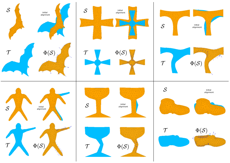
Figure 13: Additional experiments on the MPEG-7 dataset. For each experiment we show the source shape $\mathcal{S}$ and the target shape $\mathcal{T}$ as well as their initial alignment. The matched shapes $\Phi(\mathcal{S})$ in each experiment are shown together with an overlap of the taget shape and the elastic forces found by our algorithm (blue arrows). No distortion bound was added.

Figure 13 shows additional experiments on shapes taken from the MPEG-7 dataset. Here we did not add any distortion bound. The results are of good quality and show intuitive elastic forces that cause the desired deformation.

5 Discussion

In this paper we introduced a novel method for shape matching of semantically similar shapes in two dimensions. The technique is based on the observation that shapes in many scenarios depict actual physical entities and hence shape change can be measured by means of forces acting on them. We model the shapes as plane elastic bodies and measure the severity of a deformation by means of external elastic forces acting on their boundaries. Our method works on triangular meshes but of course one can use any shape representation such as polygons or point clouds to build such a mesh.

In order to describe the behavior of the shapes that we model as elastic bodies we use the theory of linearized elasticity. The relevant equations are the Navier-Lamé equations which constitute a linear system of partial differential equations with additional boundary conditions. These can be displacement conditions (Dirichlet type) and/or force conditions (Neumann type) and they are usually unknown in the context of shape matching. We show how to map displacement boundary conditions linearly to boundary forces in a FEM framework. This enables us to seek boundary displacements that supplement the Navier-Lamé equations such that their physical cause, i.e., the boundary force, is of a simple nature. As a measure of simplicity, we believe, that the sparsity of forces is a good prior since for a given object such forces can describe different articulations of that object by mostly acting on the articulated parts.

As a (dis-)similarity measure we use the area of mutual non-overlap of the source and the target shape, i.e., the area of the symmetric difference of the two shapes. This is a global measure and its minima under deformation of the source mean a maximum overlap of the shapes. This is clearly in contrast to classical ICP since a minimal mean (Euclidean) distance (under deformation of the source) can be obtained by mapping the source to a single point (without regularization).

Our algorithm is designed so that it simultaneously seeks low sparse forces and a good alignment, measured by the area of the symmetric difference. We show a heuristic way to approximate the nonlinear optimization problem by a sequence of (convex) second order cone problems that only involve the boundary of the mesh. This reduces the number of variables of the problem. We apply the algorithm to a number of examples taken from various datasets. In addition, we provide a comparison to our ICP-like method introduced in [48] and show that the new symmetric difference algorithm can outperform the ICP-like method.

Although the Navier-Lamé equations are only valid in the narrow regime of small displacements and strain we show that the symmetric difference method can find remarkably large deformations in which the ICP-like method failed. Since we use gradient information of the symmetric difference the method is, similarly to the ICP-like method, a local method that is sensitive to the initial alignment of the shapes.

Despite good alignment results the symmetric difference method can unfortunately suffer from large conformal distortions of the triangular mesh and elements can even flip. We therefore suggest a way to deal with this problem by incorporating into our optimization a method that is guaranteed to have no flipped triangles and does not exceed a distortion bound that is pre-selected by the user. Incorporating this method, which was introduced in [33], does neither change the type of the optimization problem nor its dimensionality. One simply has to add a number of second order cone constraints. The distortion bound should not be chosen too low since a low bound might exclude a good solution.

Unfortunately this algorithm does not generalize to three dimensions because the clipping algorithm does not generalize. Also, a generalization to nonlinear material models, i.e., to rotation invariant deformation cost is desirable in order to extend the applicability of the method. This is left for future research.

Acknowledgments. This research was supported by the Israel Science Foundation, Grant No. 1265/14. The vision group at the Weizmann Institute is supported in part by the Moross Laboratory for Vision Research and Robotics.

References

- [1] D. Aiger, N.J. Mitra, D. Cohen-Or 4-points Congruent Sets for Robust Surface Registration, ACM Transactions on Graphics Vol. 27, no.3 (2008)
- [2] B. Allen, B. Curless, Z. Popović The Space of Human Body Shapes: Reconstruction and Parameterization from Range Scans, ACM Transactions on Graphics Vol. 22, no. 3 (2003)
- [3] H. Alt, U. Fuchs, G. Rote, G. Weber Matching convex shapes with respect to the symmetric difference, Algorithmica 21, no. 1, pp. 89–103 (1998)
- [4] L. Ambrosio, V.M. Tortorelli Approximation of Functional Depending on Jumps by Elliptic Functional via -Convergence, Communications on Pure and Applied Mathematics, Vol. 43, no. 8, pp. 999–1036 (1990)
- [5] Y. Amit A Nonlinear Variational Problem for Image Matching, SIAM Journal on Scientific Computing Vol. 15, no. 1, 207–224 (1994)
- [6] E.D. Andersen, K.D. Andersen The Mosek Interior Point Optimizer for Linear Programming: An Implementation of the Homogeneous Algorithm, Kluwer Academic Publishers, 197–232 (1999)
- [7] R. Bajcsy, C. Broit Matching of Deformed Images, Proc. Int. Conf. Pattern Recognition, pp. 351–-353 (1982)
- [8] M.F. Beg, M.I. Miller, A. Trouvé, L. Younes Computing Large Deformation Metric Mappings via Geodesic Flows of Diffeomorphisms, International Journal of Computer Vision Vol. 61, no. 2, 139–157 (2005)
- [9] B. Berkels, G. Linkmann, M. Rumpf An -Invariant Shape Median, Journal of Mathematical Imaging Vision, Vol. 37, no. 2, pp. 85–97 (2010)
- [10] P.J. Besl, N.D. McKay A method for Registration of 3-D Shapes, IEEE Transactions on Pattern Analysis and Machine Intelligence Vol. 14, no. 2, 239–256 (1992)
- [11] M. Blank, L. Gorelick, E. Shechtman, M. Irani and R. Basri Actions as Space-Time Shape, International Conference on Computer Vision, pp. 1395–1402 (2005)
- [12] D. Braess Finite elements. Theory, fast solvers, and applications in solid mechanics, Cambridge University Press (2001)
- [13] M. Bro-Nielsen Finite Elements Modeling in Surgery Simulation, Proceedings of the IEEE Vol. 86, no. 3, March 1998
- [14] A. M. Bronstein, M. M. Bronstein, A. M. Bruckstein and R. Kimmel Analysis of two-dimensional non-rigid shapes, International Journal of Computer Vision Vol. 78, no. 1, 67–88 (2008)
- [15] A. M. Bronstein, M. M. Bronstein, M. Mahmoudi, R. Kimmel, G. Sapiro A Gromov-Hausdorff framework with diffusion geometry for topologically-robust non-rigid shape matching, International Journal of Computer Vision, Vol. 89, no. 2–3, pp. 266–286 (2010)
- [16] A.M. Bronstein, M.M. Bronstein, R. Kimmel Numerical geometry of non-rigid shapes, Springer, 2008.
- [17] B.J. Brown, S. Rusinkiewicz Global non-rigid alignment of 3-D scans, ACM Transactions on Graphics Vol. 26, no. 3 (2007)
- [18] T.F. Chan, L. Vese Active contours without edges, IEEE transactions on Image Processing, Vol. 10, no. 2, pp. 266–277 (2001)
- [19] T.F. Chan, L. Vese A level set algorithm for minimizing the Mumford-Shah functional in image processing, IEEE Workshop on Variational and Level Set Methods in Computer Vision, pp. 161–168 (2001)
- [20] P.G. Ciarlet Mathematical Elasticity. Volume I: Three-Dimensional Theory, Series “Studies in Mathematics and its Applications”, North-Holland, Amsterdam (1988)
- [21] G.E. Christensen, R.D. Rabbitt, M.I. Miller Deformable Templates Using Large Deformation Kinematics, IEEE Transactions on Image Processing Vol. 5, no. 10, 1435–1447 (1996)
- [22] G. Dhondt The Finite Element Method for Three-Dimensional Thermomechanical Applications, Wiley (2004)
- [23] M.-P. Dubuisson, A.K. Jain A modified Hausdorff distance for object matching, International Conference on Pattern Recognition, Vol. 1, pp. 566–568 (1994)
- [24] M. Ferrant, S.K. Warfield, C.R.G. Guttmann, R.V. Mulkern, F.A. Jolesz, R. Kikinis 3D Image Matching Using a Finite Element Based Elastic Deformation Model, Proceedings of MICCAI 1999, LNCS 1679, pp. 202–209 (1999)
- [25] J.C. Gee, R.K. Bajcsy Elastic Matching: Continuum Mechanical and Probabilistic Analysis, Brain Warping, Vol. 2, pp. 18–3 (1998)
- [26] N. Gelfand, N.J. Mitra, L.J. Guibas, H. Pottmann Robust Global Registration, Symposium on Geometry Processing, pp. 197–206 (2005)
- [27] G. Greiner, K. Hormann Efficient clipping of arbitrary polygons, ACM Transactions on Graphics (TOG) Vol. 17, no. 2, pp. 71–83 (1998)
- [28] M. Holden A review of geometric transformations for nonrigid body registration, IEEE Transactions on Medical Imaging Vol. 27, no. 1, pp. 111–128 (2008)
- [29] D. Huttenlocher, G. Klanderman, W. Rucklidge Comparing Images Using the Hausdorff Distance, IEEE Transactions on Pattern Analysis and Machine Intelligence, Vol. 15, 850-863 (1993)
- [30] R. Kimmel Numerical Geometry of Images: Theory, Algorithms, and Applications, Springer Verlag, 2003
- [31] S.Z. Kovalsky, N. Aigerman, R. Basri, Y. Lipman Controlling Singular Values with Semidefinite Programming, ACM Transactions on Graphics Vol. 33, no. 4 (2014)
- [32] L.J. Latecki, R. Lakämper, U. Eckhardt, Shape descriptors for non-rigid shapes with a single closed contour, IEEE Conference on Computer Vision and Pattern Recognition (CVPR), Vol. 1, pp. 424–429 (2000)
- [33] Y. Lipman Bounded Distortion Mapping Spaces for Triangular Meshes, ACM Transactions on Graphics Vol. 31, no. 4 (2012)
- [34] J. Löfberg YALMIP: A Toolbox for Modeling and Optimization in MATLAB, Proceedings of the CACSD Conference (2004), http://users.isy.liu.se/johanl/yalmip
- [35] F. Memoli On the use of Gromov–Hausdorff distances for shape comparison, Eurographics Association, pp. 81–-90 (2007)
- [36] F. Memoli Gromov–Wasserstein Distances and the Metric Approach to Object Matching, Foundations of Computational Mathematisc, Vol. 11, no. 4, pp. 417–487 (2011)
- [37] W. Mio, A. Srivastava, S. Joshi On Shape of Plane Elastic Curves, International Journal of Computer Vision Vol. 73, no. 3, pp. 307–324 (2007)
- [38] D. Mumford, J. Shah Optimal approximations by piecewise smooth functions and associated variational problems, Communications on pure and applied mathematics, Vol. 42, no. 5, pp. 577–685 (1989)
- [39] A. Murta, T. Howard The General Polygon CLipping Library GPC, http://www.cs.man.ac.uk/ toby/gpc/
- [40] A. Nealen, M. Müller, R. Keiser, E. Boxerman, M. Carlson Physically based deformable models in computer graphics, Computer Graphics Forum Vol. 25, no. 4, pp. 809–836 (2006)
- [41] N.C. Overgaard, J.E. Solem Separating rigid motion for continuous shape evolution, International Conference on Pattern Recognition 2006
- [42] W. Peckar, C. Schnörr, K. Rohr, H.S. Stiehl Parameter-Free Elastic Deformation Approach for 2D and 3D Registration Using Prescribed Displacements, J. Math. Imaging and Vision Vol. 10, no. 2, pp. 143–162 (1999)
- [43] S. Rusinkiewicz, M. Levoy Efficient variants of the ICP algorithm, Proc. of the 3rd International Conference on 3-D Digital Imaging and Modeling (2001)
- [44] M. Rumpf, B. Wirth A Nonlinear Elastic Shape Averaging Approach, SIAM Jouranl of Imaging Sciences, Vol.2, no. 3, pp. 800–833 (2009)
- [45] T.B. Sebastian, P.N. Klein and B.B. Kimia Recognition of Shapes by Editing Shock Graphs, International Conference on Computer Vision, pp. 755–762 (2001)
- [46] T.W. Sederberg, E. Greenwood A Physically Based Approach to 2-D Shape Blending, ACM SIGGRAPH Computer Graphics Vol. 26, no. 2 (1992)
- [47] J.A. Sethian Level Set Methods and Fast Marching Methods: Evolving Interfaces in Computational Geometry, Fluid Mechanics, Computer Vision, and Materials Science, Vol. 3. Cambridge University Press (1999)
- [48] K. Simon, S. Sheorey, D. Jacobs, R. Basri A Linear Elastic Force Optimization Model for Shape Matching, Journal of Mathematical Imaging and Vision (2014)
- [49] K. Simon, S. Sheorey, D. Jacobs, R. Basri A Hyperelastic Two-scale Optimization Model for Shape Matching, submitted
- [50] I.E. Sutherland, G.W. Hodgman Reentrant Polygon Clipping, Commun. ACM Vol. 17, no. 1, pp. 32–42 (1974)
- [51] D. Terzopoulos, J. Platt, A. Barr, K. Fleischer Elastically deformable models, ACM Siggraph Computer Graphics Vol. 21, no. 4, pp. 205–214 (1987).
- [52] B.R. Vatti A generic solution to polygon clipping, Communications of the ACM, Vol. 35, no. 7, pp. 56–63 (1992)
- [53] L. Younes Computable Elastic Distances Between Shapes, SIAM J. Appl. Math. Vol. 58, no. 2, pp. 565–586 (1998)
- [54] L. Younes Optimal Matching Between Shapes via Elastic Deformations, Image and Vision Computing Vol. 17, pp. 381–389 (1999)
- [55] L. Younes Spaces and manifolds of shapes in computer vision: An overview, Image and Vision Computing Vol. 30, pp. 389–397 (2012)