Lattice dynamics and electron-phonon coupling calculations using non-diagonal supercells

Abstract

We study the direct calculation of total energy derivatives for lattice dynamics and electron-phonon coupling calculations using supercell matrices with non-zero off-diagonal elements. We show that it is possible to determine the response of a periodic system to a perturbation characterized by a wave vector with reduced fractional coordinates $(m_{1}/n_{1},m_{2}/n_{2},m_{3}/n_{3})$ using a supercell containing a number of primitive cells equal to the least common multiple of $n_{1}$, $n_{2}$, and $n_{3}$. If only diagonal supercell matrices are used, a supercell containing $n_{1}n_{2}n_{3}$ primitive cells is required. We demonstrate that the use of non-diagonal supercells significantly reduces the computational cost of obtaining converged zero-point energies and phonon dispersions for diamond and graphite. We also perform electron-phonon coupling calculations using the direct method to sample the vibrational Brillouin zone with grids of unprecedented size, which enables us to investigate the convergence of the zero-point renormalization to the thermal and optical band gaps of diamond.

I Introduction

The experimental study of condensed matter usually involves measuring the response of a system to some external perturbation. Many properties of materials can be studied theoretically by the calculation of derivatives of the total energy with respect to applied perturbations, such as force constants, elastic constants, Born effective charges, and piezoelectric constants Martin (2004). First principles methods have been successfully used to study the response of a wide range of systems to a variety of perturbations Kunc and Martin (1982); Niu and Kleinman (1998); Marzari and Singh (2000); Baroni et al. (2001); Joyce et al. (2007); Ambrosetti et al. (2014), complementing or explaining experimental discoveries, and predicting novel properties and behavior.

The response of periodic systems to perturbations characterized by a wave vector can be calculated using the direct method Yin and Cohen (1980); Fleszar and Resta (1985) or perturbative methods Baroni et al. (1987); Giannozzi et al. (1991); Gonze (1997). The direct method relies on freezing a perturbation into the system and calculating the total energy derivatives using a finite difference approach. The result is a transparent formalism, but only perturbations commensurate with the simulation cell can be calculated exactly. This presents some difficulties, for example, quantities derived from electron-phonon coupling matrix elements require a fine sampling of the vibrational Brillouin zone (BZ) Giustino et al. (2007, 2010) and converged results are typically not obtainable using simulation cells of tractable sizes. Perturbative methods can access perturbations at an arbitrary wave vector using a single primitive cell, and therefore have been the method of choice for the vast majority of calculations, from phonon dispersions Giannozzi et al. (1991) and electron-phonon coupling Kong et al. (2001) to spin fluctuations Savrasov (1998).

The simplicity of the direct method means that it typically plays a central role in early calculations in a given area. For example, it was used in the first phonon calculations for materials beyond $sp$-bonded metals Chadi and Martin (1976), and the only available electron-phonon coupling calculations using many-body perturbation theory rely on this approach Lazzeri et al. (2008); Grüneis et al. (2009); Faber et al. (2011); Yin et al. (2013); Antonius et al. (2014). The direct method is also readily extendable to situations where large distortions are required, as the energy is found at all orders. It is therefore desirable to reduce the computational cost and consequently extend the range of applicability of the direct method.

In this paper, we prove that in order to calculate the response of a periodic system to a perturbation at a wave vector with reduced fractional coordinates $(m_{1}/n_{1},m_{2}/n_{2},m_{3}/n_{3})$, it is only necessary to consider a supercell containing a number of primitive cells equal to the least common multiple (LCM) of $n_{1}$, $n_{2}$, and $n_{3}$. This is accomplished by utilizing supercell matrices containing non-zero off-diagonal elements. For example, the sampling of the vibrational BZ with a uniform grid of size $N\times N\times N$ can be accomplished with supercells containing at most $N$ primitive cells. In contrast, the size of the largest supercell that may need to be considered scales cubically with the linear size of the BZ grid when only using diagonal supercell matrices.

We find that the use of non-diagonal supercell matrices reduces the computational cost of obtaining converged zero-point energies and phonon dispersions for diamond and graphite by over an order of magnitude. It also enables us to perform electron-phonon coupling calculations using the direct method with BZ grids of unprecedented size. In particular, we investigate the convergence with respect to the number of points used to sample the vibrational BZ of the zero-point renormalization to the thermal and optical band gaps of diamond, a problem that has previously been considered challenging for the direct approach due to the prohibitive computational cost of using simulation cells containing sufficient numbers of primitive cells.

The paper is organized as follows: We introduce the use of non-diagonal supercell matrices to access perturbations at a given wave vector in Sec. II. We describe the computational details of our calculations in Sec. III. We illustrate the utility of our approach in the context of first principles lattice dynamics in Sec. IV and in relation to electron-phonon coupling calculations in Sec. V. Our conclusions are drawn in Sec. VI.

II Supercells and k-point sampling

II.1 Supercell matrices

A simulation cell that contains multiple primitive cells of a given crystal lattice is known as a supercell and is itself the unit cell of a superlattice, whose basis vectors are constructed by taking linear combinations of the primitive lattice basis vectors with integer coefficients Santoro and Mighell (1972). This can be expressed algebraically as

$$\begin{pmatrix}\mathbf{a}_{\text{s}_{1}}\\ \mathbf{a}_{\text{s}_{2}}\\ \mathbf{a}_{\text{s}_{3}}\end{pmatrix}=\begin{pmatrix}S_{11}&S_{12}&S_{13}\\ S_{21}&S_{22}&S_{23}\\ S_{31}&S_{32}&S_{33}\end{pmatrix}\begin{pmatrix}\mathbf{a}_{\text{p}_{1}}\\ \mathbf{a}_{\text{p}_{2}}\\ \mathbf{a}_{\text{p}_{3}}\end{pmatrix}\,,$$ (1)

where $\mathbf{a}_{\text{s}_{i}}$ are the superlattice basis vectors, $\mathbf{a}_{\text{p}_{i}}$ are the primitive lattice basis vectors, and $S_{ij}\in\mathbb{Z}$. The supercell contains $|S|$ primitive cells and we refer to the matrix $S$ as the supercell matrix. For the purposes of brevity, we shall henceforth refer to supercells generated by diagonal supercell matrices as diagonal supercells and those generated by non-diagonal supercell matrices as non-diagonal supercells.

The set of wave vectors that describe plane waves with the same periodicity as the primitive lattice define the reciprocal primitive lattice with basis vectors

$$\begin{pmatrix}\mathbf{b}_{\text{p}_{1}}\\ \mathbf{b}_{\text{p}_{2}}\\ \mathbf{b}_{\text{p}_{3}}\end{pmatrix}=2\pi\begin{pmatrix}\mathbf{a}_{\text{p}_{1}}\\ \mathbf{a}_{\text{p}_{2}}\\ \mathbf{a}_{\text{p}_{3}}\end{pmatrix}^{-\text{T}}\,,$$ (2)

and the set of wave vectors that describe plane waves with the same periodicity as the superlattice define the reciprocal superlattice with basis vectors

$$\begin{pmatrix}\mathbf{b}_{\text{s}_{1}}\\ \mathbf{b}_{\text{s}_{2}}\\ \mathbf{b}_{\text{s}_{3}}\end{pmatrix}=\begin{pmatrix}\bar{S}_{11}&\bar{S}_{12}&\bar{S}_{13}\\ \bar{S}_{21}&\bar{S}_{22}&\bar{S}_{23}\\ \bar{S}_{31}&\bar{S}_{32}&\bar{S}_{33}\end{pmatrix}\begin{pmatrix}\mathbf{b}_{\text{p}_{1}}\\ \mathbf{b}_{\text{p}_{2}}\\ \mathbf{b}_{\text{p}_{3}}\end{pmatrix}\,,$$ (3)

where $\bar{S}_{ij}=(S^{-1})_{ji}$. An arbitrary $\mathbf{k}$-point can be expressed in terms of both the reciprocal primitive lattice basis vectors and reciprocal superlattice basis vectors, and these fractional coordinates are related by

$$\begin{pmatrix}k_{\text{s}_{1}}\\ k_{\text{s}_{2}}\\ k_{\text{s}_{3}}\end{pmatrix}=\begin{pmatrix}S_{11}&S_{12}&S_{13}\\ S_{21}&S_{22}&S_{23}\\ S_{31}&S_{32}&S_{33}\end{pmatrix}\begin{pmatrix}k_{\text{p}_{1}}\\ k_{\text{p}_{2}}\\ k_{\text{p}_{3}}\end{pmatrix}\,.$$ (4)

If the reciprocal superlattice fractional coordinates are all integers, perturbations characterized by the wave vector $\mathbf{k}$ are commensurate with the supercell generated by $S$.

There are a finite number of unique superlattices whose supercells contain a given number of primitive cells, but there are an infinite number of sets of basis vectors that can be used to describe each superlattice. Two different supercell matrices $S$ and $S^{\prime}$ generate different bases for the same superlattice if $S^{\prime}$ can be reduced to $S$ by elementary unimodular row operations Hart and Forcade (2008), which consist of the following:

• Adding an integer multiple of one row of the matrix to another row.

• Interchanging two rows of the matrix.

• Multiplying a row of the matrix by $-1$.

The canonical form for such operations is the upper-triangular Hermite normal form (HNF):

$$\begin{pmatrix}S_{11}&S_{12}&S_{13}\\ 0&S_{22}&S_{23}\\ 0&0&S_{33}\end{pmatrix},\,$$ (5)

with $0\leq S_{12}<S_{22}$ and $0\leq S_{13},S_{23}<S_{33}$. This means that all inequivalent supercell matrices can be written in the form given by Eq. (5). Note that the product $S_{11}S_{22}S_{33}$ fixes the determinant $|S|$ and therefore the number of primitive cells contained within the supercell.

II.2 Commensurate supercells

We now show that a $\mathbf{k}$-point with fractional coordinates

$$\begin{pmatrix}k_{\text{p}_{1}}\\ k_{\text{p}_{2}}\\ k_{\text{p}_{3}}\end{pmatrix}=\begin{pmatrix}\frac{m_{1}}{n_{1}}\\ \frac{m_{2}}{n_{2}}\\ \frac{m_{3}}{n_{3}}\end{pmatrix}\,,$$ (6)

where $0\leq k_{\text{p}_{1}},k_{\text{p}_{2}},k_{\text{p}_{3}}<1$ and $m_{1}/n_{1}$, $m_{2}/n_{2}$, and $m_{3}/n_{3}$ are reduced fractions, is commensurate with a supercell containing $l_{123}$ primitive cells, where $l_{123}$ is the LCM of $n_{1}$, $n_{2}$, and $n_{3}$. That is to say, we are able to solve the equations

$$k_{\text{s}_{1}} =\frac{S_{11}m_{1}}{n_{1}}+\frac{S_{12}m_{2}}{n_{2}}+\frac{S_{13}m_{3}}{n_{3}}$$ (7)

$$k_{\text{s}_{2}} =\frac{S_{22}m_{2}}{n_{2}}+\frac{S_{23}m_{3}}{n_{3}}$$ (8)

$$k_{\text{s}_{3}} =\frac{S_{33}m_{3}}{n_{3}}$$ (9)

for integer $k_{\text{s}_{1}}$, $k_{\text{s}_{2}}$, and $k_{\text{s}_{3}}$ with $S_{11}S_{22}S_{33}=l_{123}$ and $S_{12}$, $S_{13}$, and $S_{23}$ satisfying the conditions stated above. The proof that follows uses properties of complete and reduced residue systems, which are detailed in the Appendix.

We trivially solve Eq. (9) by setting $S_{33}=n_{3}$. We solve Eq. (8) by setting $S_{22}=n_{2}/g_{23}$ and $S_{23}=pn_{3}/g_{23}$, where $g_{23}$ is the greatest common divisor (GCD) of $n_{2}$ and $n_{3}$, and $p$ is a non-negative integer, which results in

$$k_{\text{s}_{2}}=\frac{m_{2}}{g_{23}}+\frac{pm_{3}}{g_{23}}.$$ (10)

The condition $S_{23}<S_{33}$ requires that $p<g_{23}$. If $g_{23}=1$, $p=0$, and if $g_{23}>1$, $m_{3}\,\text{mod}\,g_{23}$ is a generator for the additive group of integers modulo $g_{23}$. This follows since $m_{3}/n_{3}$ is a reduced fraction and $g_{23}$ divides $n_{3}$. We can therefore always choose $p<g_{23}$ such that $(m_{2}+pm_{3})\,\text{mod}\,g_{23}=0$ and obtain an integer solution for $k_{\text{s}_{2}}$.

We now consider Eq. (7) and proceed by setting $S_{11}=g_{123}n_{1}/(g_{12}g_{31})$, $S_{12}=qg_{123}n_{2}/(g_{12}g_{23})$, and $S_{13}=rg_{123}n_{3}/(g_{31}g_{23})$, where $g_{12}$ is the GCD of $n_{1}$ and $n_{2}$, $g_{31}$ is the GCD of $n_{3}$ and $n_{1}$, $g_{123}$ is the GCD of $n_{1}$, $n_{2}$, and $n_{3}$, and $q$ and $r$ are non-negative integers, which results in

$$\begin{split}k_{\text{s}_{1}}=&\phantom{+}\frac{g_{123}}{g_{31}g_{23}}\left[\frac{(g_{23}/g_{123})m_{1}}{g_{12}/g_{123}}+\frac{q(g_{31}/g_{123})m_{2}}{g_{12}/g_{123}}\right]\\ &+\frac{rg_{123}m_{3}}{g_{31}g_{23}}\,.\end{split}$$ (11)

The condition $S_{12}<S_{22}$ requires that $q<g_{12}/g_{123}$ and the condition $S_{13}<S_{33}$ requires that $r<g_{31}g_{23}/g_{123}$. If $g_{12}/g_{123}=1$, $q=0$, and if $g_{12}/g_{123}>1$, $m_{2}\,\text{mod}\,(g_{12}/g_{123})$ is an element of the multiplicative group of integers modulo $g_{12}/g_{123}$. This follows since $m_{2}/n_{2}$ is a reduced fraction, $g_{12}$ divides $n_{2}$, and $g_{123}$ divides $g_{12}$. $(g_{31}/g_{123})\,\text{mod}\,(g_{12}/g_{123})$ is also an element of the multiplicative group of integers modulo $g_{12}/g_{123}$. This follows since $g_{123}$ is the GCD of $g_{12}$ and $g_{31}$, which means that $(g_{31}/g_{123})/(g_{12}/g_{123})$ is a reduced fraction. The product $(g_{31}/g_{123})m_{2}\,\text{mod}\,(g_{12}/g_{123})$ is a generator for the additive group of integers modulo $g_{12}/g_{123}$ and we can therefore always choose $q<g_{12}/g_{123}$ such that $((g_{23}/g_{123})m_{1}+q(g_{31}/g_{123})m_{2})\,\text{mod}\,(g_{12}/g_{123})=0$. Both of these cases lead to

$$k_{\text{s}_{1}}=\frac{z}{g_{31}g_{23}/g_{123}}+\frac{rm_{3}}{g_{31}g_{23}/g_{123}}\,,$$ (12)

where $z$ is an integer. If $g_{31}g_{23}/g_{123}=1$, $r=0$, and if $g_{31}g_{23}/g_{123}>1$, $m_{3}\,\text{mod}\,(g_{31}g_{23}/g_{123})$ is a generator for the additive group of integers modulo $g_{31}g_{23}/g_{123}$. This follows since $m_{3}/n_{3}$ is a reduced fraction, $g_{31}$ and $g_{23}$ both divide $n_{3}$, and $g_{123}$ divides both $g_{31}$ and $g_{23}$. We can therefore always choose $r<g_{31}g_{23}/g_{123}$ such that $(z+rm_{3})\,\text{mod}\,(g_{31}g_{23}/g_{123})=0$ and obtain an integer solution for $k_{\text{s}_{1}}$.

Given the choice of $S_{11}$, $S_{22}$, and $S_{33}$ stated above, the number of primitive cells contained within the supercell is $g_{123}n_{1}n_{2}n_{3}/g_{12}g_{23}g_{31}=l_{123}$. In particular, we can access all $\mathbf{k}$-points on a uniform $N\times N\times N$ grid by considering supercells containing at most $N$ primitive cells.

II.3 Two-dimensional example

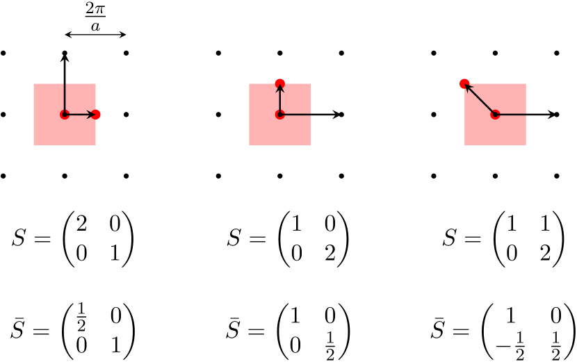
Figure 1: (color online) Example of the use of non-diagonal supercells to access all points on a $2\times 2$ grid sampling the BZ (red shaded area) of a square lattice (black dots). The black arrows indicate the reciprocal superlattice vectors and the red dots indicate the points in the first BZ that are accessible to them.

We now describe a two-dimensional example of the use of non-diagonal supercells to access any point on a $2\times 2$ grid sampling the BZ of a square lattice with spacing $a$. The reciprocal lattice is also square, but with lattice parameter $2\pi/a$.

In Fig. 1, we show the reciprocal lattice together with the first BZ (shaded red area). The points of a $2\times 2$ grid on the BZ have fractional coordinates $(0,0)$, $(\frac{1}{2},0)$, $(0,\frac{1}{2})$, and $(\frac{1}{2},\frac{1}{2})$. The centre of the BZ, $(0,0)$, is commensurate with a primitive cell. Diagonal supercells with $|S|=2$ may be used to access the points $(\frac{1}{2},0)$ and $(0,\frac{1}{2})$, as shown in Fig. 1. The point $(\frac{1}{2},\frac{1}{2})$ cannot be accessed with a diagonal supercell of size $|S|=2$, and instead the smallest diagonal supercell that provides access to this point has size $|S|=4$. However, as shown in Fig. 1, a non-diagonal supercell of size $|S|=2$ provides access to the point $(-\frac{1}{2},\frac{1}{2})$, which is equivalent to the point $(\frac{1}{2},\frac{1}{2})$.

II.4 Other uses of non-diagonal supercells

Non-diagonal supercells have been previously used for the calculation of phonon dispersion curves along high symmetry lines using the planar force constant method Yin and Cohen (1982); Kunc and Dacosta (1985). In this context, supercells are constructed by hand to capture the force constants arising from finite displacements of entire planes of atoms. Interatomic force constants may, in principle, be obtained from a set of such interplanar force constants using a least-squares fit procedure Wei and Chou (1992). A similar procss may be carried out using a combination of supercells that maximizes the cutoff radius of the force constants Heid et al. (1998). In Sec. IV below, we show how non-diagonal supercells can be used to directly construct the dynamical matrices required for lattice dynamics calculations in the harmonic approximation, thus generalizing and systematizing previous approaches.

More widely, non-diagonal supercells have been used in real space methods such as quantum Monte Carlo for the study of solids from first principles Foulkes et al. (2001); Drummond et al. (2015), or the Lanczos method for the study of model systems Dagotto (1994); Kent et al. (2005). In these cases, non-diagonal supercells are used to construct appropriate simulation cells to facilitate the extrapolation of finite system size results to the infinite system limit, as well as for the calculation of total energy derivatives to evaluate susceptibilities.

III Computational details

III.1 Non-diagonal supercell generation

We now describe how we use non-diagonal supercells to perform calculations of total energy derivatives using the direct method in practice. We express each $\mathbf{k}$-point of interest in reduced fractional coordinates and calculate $l_{123}$ to determine the size of supercell $|S|$ commensurate with it. We choose the appropriate supercell matrix in HNF and then perform elementary unimodular row operations on it until the superlattice basis vectors are the shortest possible. We have found this to reduce the total number of points required to sample the electronic BZ for a fixed Monkhorst-Pack Monkhorst and Pack (1976) grid spacing criterion, which helps to minimize the computational cost of our first principles calculations. A fortran 90 program implementing this procedure is included in the Supplemental Material Sup .

III.2 First principles calculations

We have studied diamond and graphite using plane wave pseudopotential density functional theory Hohenberg and Kohn (1964); Kohn and Sham (1965), as implemented in version 8 of the castep code Clark et al. (2005). We used the local density approximation Ceperley and Alder (1980); Perdew and Zunger (1981) to the exchange-correlation functional and an “on-the-fly” ultrasoft pseudopotential Vanderbilt (1990) generated by castep with valence states $2\text{s}^{2}2\text{p}^{2}$. We used a plane wave energy cutoff of $800$ eV and sampled the electronic BZ with a Monkhorst-Pack Monkhorst and Pack (1976) grid of density $2\pi\times 0.03$ Å^-1, which was sufficient to converge the energy differences between different frozen phonon configurations to better than $10^{-4}$ eV per atom. We relaxed the structures at zero pressure until the forces on each atom were smaller than $10^{-4}$ eV/Å and the components of the stress tensor were smaller than $10^{-4}$ GPa, which resulted in a lattice constant of $3.532$ Å for diamond, and an in-plane lattice parameter of $2.445$ Å with $c/a=2.707$ for graphite. These values are slightly smaller than the experimental ones Judith Grenville-Wells and Lonsdale (1958); Hanfland et al. (1989); Zhao and Spain (1989), which is because the local density approximation favors uniform charge densities and therefore tends to overbind. The lattice constant of diamond is also different to that obtained with version 7 of castep used for Ref. Monserrat and Needs, 2014, which is due to a change in the default “on-the-fly” pseudopotential.

IV Lattice dynamics

IV.1 Formalism

Assuming Born-von Karman periodic boundary conditions Born and Huang (1956) applied to an $N_{1}\times N_{2}\times N_{3}$ array of primitive cells, the central question of first principles lattice dynamics in the harmonic approximation Wallace (1972) is how to determine the so-called dynamical matrix at each $\mathbf{k}$-point on an $N_{1}\times N_{2}\times N_{3}$ grid sampling the vibrational BZ. The dynamical matrix is defined as

$$D_{ij}(\alpha\beta\,|\,\mathbf{k})=\frac{1}{\sqrt{m_{\alpha}m_{\beta}}}\sum_{\mathbf{R}_{p}}\Phi_{ij}(\alpha\beta\,|\,\mathbf{R}_{p})\text{e}^{-\text{i}\mathbf{k}\cdot\mathbf{R}_{p}}\,,$$ (13)

where Latin indices label Cartesian coordinates, Greek indices label the atoms within a primitive cell, $m_{\alpha}$ is the mass of atom $\alpha$, $\mathbf{R}_{p}$ are the position vectors of the primitive cells that make up the simulation cell, and

$$\Phi_{ij}(\alpha\beta\,|\,\mathbf{R}_{p}-\mathbf{R}_{p^{\prime}})=\frac{\partial^{2}E_{\text{BO}}}{\partial u_{i}(\alpha\,|\,\mathbf{R}_{p})\partial u_{j}(\beta\,|\,\mathbf{R}_{p^{\prime}})}\,,$$ (14)

where $E_{\text{BO}}$ is the Born-Oppenheimer (BO) potential energy surface Born and Oppenheimer (1927) and $u_{i}(\alpha\,|\,\mathbf{R}_{p})$ is the $i$th component of the displacement from its equilibrium position of the $\alpha$th atom in the primitive cell located at $\mathbf{R}_{p}$, is the matrix of interatomic force constants. The eigenvectors of the dynamical matrix can be used to rewrite the harmonic vibrational Hamiltonian in terms of normal coordinates $q_{n\mathbf{k}}$, where $n$ is the phonon branch index. The Hamiltonian then takes the form of a sum of terms corresponding to non-interacting simple harmonic oscillators with frequencies $\omega_{n\mathbf{k}}$ equal to the square root of the eigenvalues of the dynamical matrix. The resulting vibrational eigenstates can be found analytically.

The matrix of force constants decays with distance between primitive cells and consequently it is possible to obtain an excellent approximation to the exact dynamical matrix at an arbitrary wave vector if the simulation cell is sufficiently large Yin and Cohen (1982). Therefore, the standard approach is to determine the dynamical matrix at each symmetry-inequivalent $\mathbf{k}$-point on the $N_{1}\times N_{2}\times N_{3}$ grid (typically referred to as the coarse grid), construct the matrix of force constants corresponding to the $N_{1}\times N_{2}\times N_{3}$ array of primitive cells using the inverse of Eq. (13), and then calculate phonon frequencies and atomic displacement patterns at a large number of $\mathbf{k}$-points, which can be used to compute structural, vibrational, and thermodynamic properties of the system. The first step of this process can be achieved either by using density functional perturbation theory Baroni et al. (2001) to determine the linear response of the charge density to an atomic displacement characterized by a wave vector $\mathbf{k}$, or by directly calculating the matrix of force constants using a supercell commensurate with $\mathbf{k}$ and performing the Fourier transform given by Eq. (13). The direct approach takes advantage of the fact that the dynamical matrix is exact at a given $\mathbf{k}$-point, in the sense that it is equal to its infinite system counterpart, if it is constructed using force constants calculated with a supercell commensurate with the wave vector $\mathbf{k}$. It is convenient to restrict the exact calculation of the dynamical matrix to $\mathbf{k}$-points in the irreducible wedge of the BZ (IBZ) and obtain it at all other points by exploiting the crystal symmetries Maradudin and Vosko (1968). Numerical noise can slightly break the symmetry of the dynamical matrix elements at each wave vector but this is corrected by symmetrizing them with respect to the point group operations of the crystal that leave the wave vector unchanged Worlton and Warren (1972).

IV.2 Results

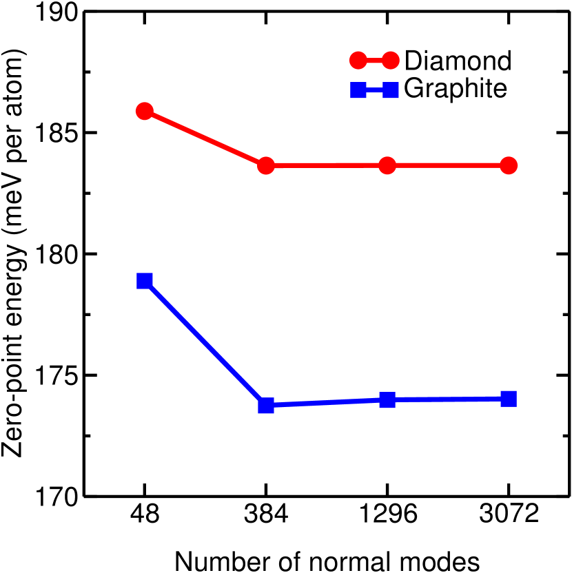
Figure 2: (color online) Zero-point energy as a function of the number of normal modes (coarse grid size) for diamond (red circles) and graphite (blue squares). The solid lines are a guide to the eye.

In Fig. 2, we show the convergence with respect to the number of normal modes included on the coarse grid used to sample the vibrational BZ of the zero-point energy for diamond and graphite. The zero-point energy is converged to better than $0.1$ meV per atom using a $4\times 4\times 4$ grid with $384$ normal modes for diamond and a $6\times 6\times 3$ grid with $1,296$ normal modes for graphite.

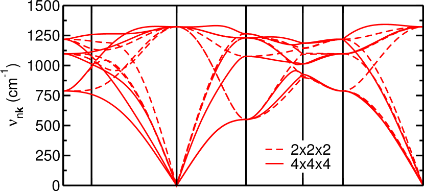
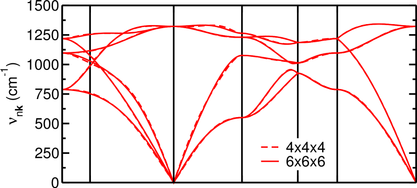
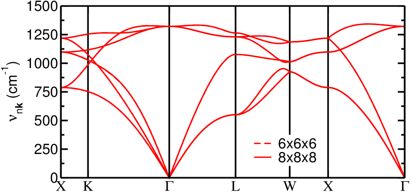
Figure 3: (color online) Convergence with respect to coarse grid size of phonon dispersions along symmetry lines for diamond.

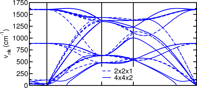
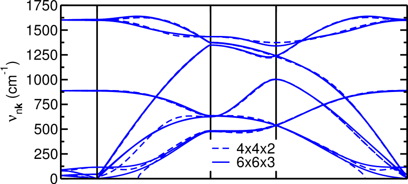
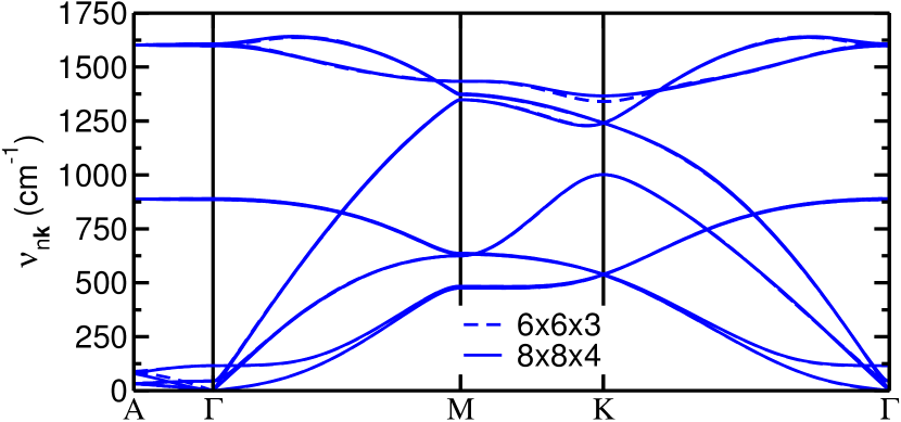
Figure 4: (color online) Convergence with respect to coarse grid size of phonon dispersions along symmetry lines for graphite.

We have also investigated the convergence of phonon dispersion relations along lines between high symmetry points in the vibrational BZ, as shown in Figs. 3 and 4. With the exception of acoustic branches in the immediate vicinity of $\Gamma$, which have negligible frequencies and are absolutely converged to better than $5~{}\text{cm}^{-1}$, we find that the phonon dispersions are converged to $1-2\%$ using a $4\times 4\times 4$ grid for diamond and a $6\times 6\times 3$ grid for graphite.

Table 1: Comparison of total computational cost of calculating force constants for diamond and graphite in order to construct the dynamical matrix at different grid sizes when using diagonal and non-diagonal supercells.

Diamond	Grid	Ratio of CPU time
		(Diagonal : Non-diagonal)
	$2\times 2\times 2$	$2.23$
	$4\times 4\times 4$	$15.3$
	$6\times 6\times 6$	$16.8$
Graphite	Grid	Ratio of CPU time
		(Diagonal : Non-diagonal)
	$2\times 2\times 1$	$1.15$
	$4\times 4\times 2$	$5.29$
	$6\times 6\times 3$	$13.8$

In Table 1, we compare the computational cost when using diagonal and non-diagonal supercells of obtaining the dynamical matrix at all $\mathbf{k}$-points in the IBZ for diamond and graphite, respectively. The use of a non-diagonal supercell can reduce the symmetry of the superlattice, which determines the number of atomic displacements required to obtain the full matrix of force constants. However, the ability to perform the necessary calculations at smaller systems sizes when using non-diagonal supercells results in a lower overall computational cost. More detailed timing information is included in the Supplemental Material Sup .

Considering diamond with a $4\times 4\times 4$ coarse grid, the most expensive calculation is that required to determine the dynamical matrix at the fractional $\mathbf{k}$-point $(1/4,1/2,-1/4)$. This can be achived by employing a diagonal $4\times 2\times 4$ supercell containing $32$ primitive cells. Therefore, the full $4\times 4\times 4$ supercell does not actually need to be constructed, as it is computationally cheaper to calculate the dynamical matrices at all points in the IBZ using multiple diagonal supercells. When using non-diagonal supercells, the largest supercells required contain just $4$ primitive cells, and the overall speedup is greater than a factor of ten.

Considering graphite with a $6\times 6\times 3$ coarse grid, the most expensive calculation is that required to determine the dynamical matrix at the fractional $\mathbf{k}$-point $(1/6,1/6,1/3)$. In this case, a diagonal $6\times 6\times 3$ supercell containing $108$ primitive cells must be constructed, which generates the force constants required to calculate the dynamical matrices at all points in the IBZ that are not present on the smaller grids. When using multiple non-diagonal supercells, the largest supercells required contain just $6$ primitive cells, and the overall speedup is greater than a factor of ten.

For both the zero-point energy and phonon dispersion relations, converged results are obtained using a $4\times 4\times 4$ coarse grid for diamond and a $6\times 6\times 3$ coarse grid for graphite. As shown in table 1, the cost of performing these calculations is reduced by over an order of magnitude when non-diagonal supercells are used instead of only diagonal supercells.

The harmonic approximation relies on the assumption that the displacement of atoms from their equilibrium positions is sufficiently small for the BO potential energy surface to be accurately approximated by a Taylor series expansion around the equilibrium atomic configuration that is truncated at second order. Therefore, it breaks down when the atomic vibrational amplitudes are large. A number of different approaches based on the direct method have recently been proposed for studying anharmonicity in solids from first principles Souvatzis et al. (2008); Hellman et al. (2011); Antolin et al. (2012); Monserrat et al. (2013); Errea et al. (2014). A common feature of these methods is that they require the sampling of the BO potential energy surface at a large number of atomic configurations, which is a process that may be greatly expedited by the use of non-diagonal supercells.

V Electron-phonon coupling

V.1 Formalism

The effect of electron-phonon coupling on the band gap of a semiconductor can be calculated by determining the change in the electronic band structure due to the displacement of atoms from their equilibrium positions Allen and Heine (1976); Allen and Cardona (1981). We calculate the vibrationally averaged band gap $\langle E_{\text{g}}\rangle$ at zero temperature in the BO approximation as

$$\langle E_{\text{g}}\rangle=\int\text{d}\mathbf{q}\,|\Phi(\mathbf{q})|^{2}\,E_{\text{g}}(\mathbf{q})\,,$$ (15)

where $\mathbf{q}$ is a collective vibrational coordinate with elements $q_{n\mathbf{k}}$ and $\Phi(\mathbf{q})$ is the vibrational wave function. Within the harmonic approximation, $\Phi(\mathbf{q})$ is a product over normal modes of simple harmonic oscillator eigenstates. The expression in Eq. (15) can be evaluated using Monte Carlo sampling Patrick and Giustino (2013); Monserrat et al. (2014), molecular dynamics Pan et al. (2014), path integral methods Ramírez et al. (2006); Morales et al. (2013), or by using a series expansion of the form Allen and Heine (1976); Allen and Cardona (1981); Giustino et al. (2010); Monserrat et al. (2013); Han and Bester (2013); Monserrat and Needs (2014)

$$E_{\text{g}}(\mathbf{q})=E_{\text{g}}(\mathbf{0})+\sum_{n,\mathbf{k}}c_{n\mathbf{k}}^{(1)}q_{n\mathbf{k}}+\sum_{\begin{subarray}{c}n,\mathbf{k}\\ n^{\prime},\mathbf{k}^{\prime}\end{subarray}}c_{n\mathbf{k}\,n^{\prime}\mathbf{k}^{\prime}}^{(2)}q_{n\mathbf{k}}q_{n^{\prime}\mathbf{k}^{\prime}}\,,$$ (16)

where we have retained terms up to second order. Within the harmonic approximation, the vibrational wave function is even and the only non-zero terms in the expectation value of Eq. (15) using the expression given by Eq. (16) are the quadratic diagonal terms with coupling constants $c_{n\mathbf{k}\,n\mathbf{k}}^{(2)}$. Within the BO approximation, the coupling constants are independent of temperature and we therefore focus on the zero-point renormalization (ZPR) to the band gap, which can be written as

$$E_{\text{ZPR}}=\sum_{n,\mathbf{k}}\frac{c_{n\mathbf{k}\,n\mathbf{k}}^{(2)}}{2\omega_{n\mathbf{k}}}.$$ (17)

This expression excludes terms with powers of $q_{n\mathbf{k}}$ higher than two and any description of coupling between different vibrational modes, but it has been found to produce good agreement with experimental results for a range of materials Antonius et al. (2014); Giustino et al. (2010); Han and Bester (2013).

V.2 Results

We used the harmonic wave functions, obtained as described in Sec. IV, to determine each $c_{n\mathbf{k}\,n\mathbf{k}}^{(2)}$ by performing frozen phonon calculations for each of the $\mathbf{k}$-points in the IBZ. The frozen phonon calculations for the vibrational mode labelled ($n,\mathbf{k}$) were performed using a vibrational amplitude of magnitude $\sqrt{\langle q_{n\mathbf{k}}^{2}\rangle}/2$, and we averaged over positive and negative displacements.

In Fig. 5, we show the ZPR to the thermal and optical band gaps of diamond as a function of the linear size of the BZ grid. It is well-known that these quantities converge slowly with respect to the number of points used to sample the vibrational BZ Giustino et al. (2010) and highly converged results have previously only been obtained using perturbative methods. The largest grids explored so far using the direct method for diamond are of sizes $4\times 4\times 4$ Antonius et al. (2014) and $6\times 6\times 6$ Monserrat and Needs (2014). Here, we report results calculated using vibrational BZ grids of size up to $48\times 48\times 48$, vastly increasing the capabilities of the direct method for this type of calculation. We find that the ZPR to the thermal gap converges within $1$ meV to a value of $-343$ meV at a grid size of $24\times 24\times 24$. The ZPR to the optical gap has a value of about $-430$ meV at a grid size of $48\times 48\times 48$ and this value differs by $15$ meV from that calculated using a $32\times 32\times 32$ grid.

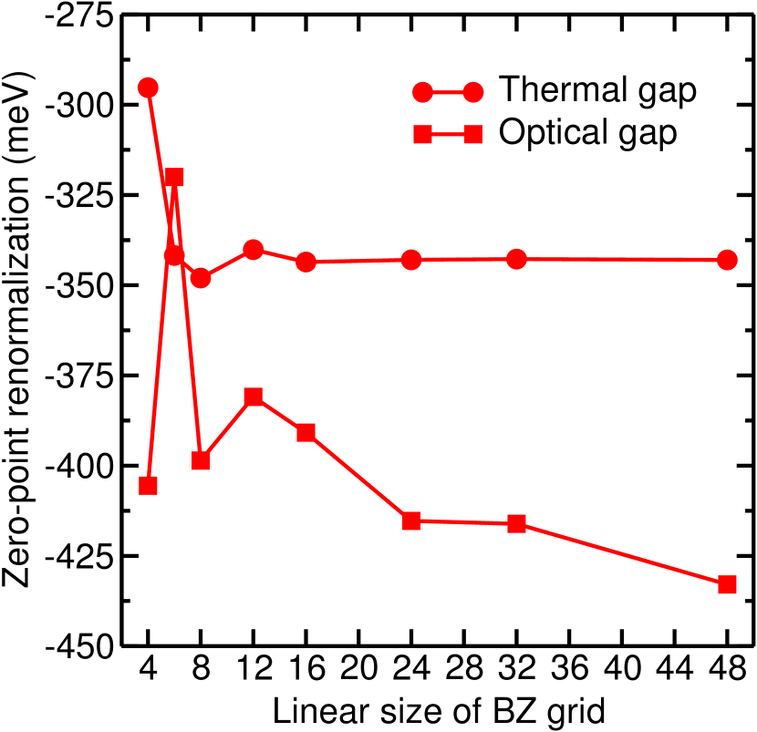
Figure 5: (color online) ZPR to the thermal (red circles) and optical (red squares) band gaps of diamond as a function of the linear size of the BZ grid. The solid lines are a guide to the eye.

We have shown that we are able to use the direct method to calculate a value of the ZPR to the thermal band gap of diamond that is converged to better than $1$ meV with respect to the number of points used to sample the vibrational BZ. The ZPR to the optical gap converges more slowly, and the results from the largest grids we consider have an uncertainty about an order of magnitude greater, of the order of $10$ meV. The choice of pseudopotential Poncé et al. (2014), higher-order terms in Eq. (16) Monserrat et al. (2014), and many-body effects Antonius et al. (2014) are known to change the values of the ZPR by amounts greater than these levels of convergence. The computational cost of investigating some of these effects may also be greatly reduced by the use of non-diagonal supercells.

VI Conclusions

We have described the use of non-diagonal supercells to study the response of periodic systems to perturbations characterized by a wave vector. We have shown that, for a wave vector with reduced fractional coordinates $(m_{1}/n_{1},m_{2}/n_{2},m_{3}/n_{3})$, there exists a commensurate supercell containing a number of primitive cells equal to the least common multiple of $n_{1}$, $n_{2}$, and $n_{3}$. This compares favourably with the $n_{1}n_{2}n_{3}$ primitive cells required if only diagonal supercells are used.

We have compared the use of diagonal and non-diagonal supercells for performing first principles lattice dynamics calculations using the direct method. We find over an order of magnitude reduction in the computational cost of obtaining converged zero-point energies and phonon dispersions for diamond and graphite when using non-diagonal supercells. We have also investigated the zero-point renormalization to the thermal and optical band gaps of diamond arising from electron-phonon coupling. Utilizing non-diagonal supercells has allowed us to perform these calculations with Brillouin zone grids of sizes up to $48\times 48\times 48$. Our results show unprecedented levels of convergence for the values of the zero-point renormalization to the thermal and optical gaps calculated using the direct method, of the orders of $1$ meV and $10$ meV, respectively.

The responses of condensed matter systems to perturbations characterized by a wave vector are central in probing a wide range of physical properties, such as phonon dispersions Giannozzi et al. (1991), electron-phonon coupling Kong et al. (2001), spin fluctuations Savrasov (1998), nuclear magnetic resonance $J$-coupling Joyce et al. (2007), and many-body dispersion effects Ambrosetti et al. (2014). Perturbative methods have provided a computationally efficient manner of determining these responses using first principles methods. The direct method has previously been considered computationally expensive due to the need to use simulation cells containing multiple primitive cells. However, it is more transparent, easier to implement in computer codes, and can be used in situations when it is necessary to go beyond the linear response regime. The use of non-diagonal supercells described in this paper significantly reduces the computational cost of the direct method, and therefore expands its applicability to problems that were previously only tractable using perturbative methods.

All relevant data present in this article can be accessed at: https://www.repository.cam.ac.uk/handle/1810/251429.

*

Appendix A Complete and reduced residue systems

Here we summarize some properties of complete and reduced residue systems. Further details can be found in Ref. Vinogradov, 1954.

If $a\,\text{mod}\,n=b\,\text{mod}\,n$, then $a$ is said to be congruent to $b$ modulo $n$.

Numbers which are congruent modulo $n$ form an equivalence class modulo $n$.

Any member of an equivalence class is said to be a residue modulo $n$ with respect to all the members of the equivalence class. Taking one residue from each equivalence class, we obtain a complete residue system modulo $n$.

If the GCD of $a$ and $n$ is equal to unity, and $x$ runs over a complete residue system modulo $n$, then $ax$ also runs over a complete residue system modulo $n$. $a$ is therefore a generator for the additive group of integers modulo $n$.

The members of an equivalence class modulo $n$ all have the same GCD relative to the modulus. Taking one residue from each class for which the GCD relative to the modulus is equal to unity, we obtain a reduced residue system modulo $n$.

If the GCD of $a$ and $n$ is equal to unity, and $x$ runs over a reduced residue system modulo $n$, then $ax$ also runs over a reduced residue system modulo $n$. $ax$ is therefore a generator for the additive group of integers modulo $n$.

References

- Martin (2004) R. M. Martin, Electronic Structure: Basic Theory and Practical Methods (Cambridge University Press, Cambridge, 2004).
- Kunc and Martin (1982) K. Kunc and R. M. Martin, “Ab initio force constants of GaAs: A new approach to calculation of phonons and dielectric properties,” Phys. Rev. Lett. 48, 406–409 (1982).
- Niu and Kleinman (1998) Q. Niu and L. Kleinman, “Spin-wave dynamics in real crystals,” Phys. Rev. Lett. 80, 2205–2208 (1998).
- Marzari and Singh (2000) N. Marzari and D. J. Singh, “Dielectric response of oxides in the weighted density approximation,” Phys. Rev. B 62, 12724–12729 (2000).
- Baroni et al. (2001) S. Baroni, S. de Gironcoli, A. Dal Corso, and P. Giannozzi, “Phonons and related crystal properties from density-functional perturbation theory,” Rev. Mod. Phys. 73, 515–562 (2001).
- Joyce et al. (2007) S. A. Joyce, J. R. Yates, C. J. Pickard, and F. Mauri, “A first principles theory of nuclear magnetic resonance J-coupling in solid-state systems,” J. Chem. Phys. 127, 204107 (2007).
- Ambrosetti et al. (2014) A. Ambrosetti, A. M. Reilly, R. A. DiStasio, and A. Tkatchenko, “Long-range correlation energy calculated from coupled atomic response functions,” J. Chem. Phys. 140, 18A508 (2014).
- Yin and Cohen (1980) M. T. Yin and M. L. Cohen, “Microscopic theory of the phase transformation and lattice dynamics of Si,” Phys. Rev. Lett. 45, 1004–1007 (1980).
- Fleszar and Resta (1985) A. Fleszar and R. Resta, “Dielectric matrices in semiconductors: A direct approach,” Phys. Rev. B 31, 5305–5310 (1985).
- Baroni et al. (1987) S. Baroni, P. Giannozzi, and A. Testa, “Green’s-function approach to linear response in solids,” Phys. Rev. Lett. 58, 1861–1864 (1987).
- Giannozzi et al. (1991) P. Giannozzi, S. de Gironcoli, P. Pavone, and S. Baroni, “Ab initio calculation of phonon dispersions in semiconductors,” Phys. Rev. B 43, 7231–7242 (1991).
- Gonze (1997) X. Gonze, “First-principles responses of solids to atomic displacements and homogeneous electric fields: Implementation of a conjugate-gradient algorithm,” Phys. Rev. B 55, 10337–10354 (1997).
- Giustino et al. (2007) F. Giustino, M. L. Cohen, and S. G. Louie, “Electron-phonon interaction using Wannier functions,” Phys. Rev. B 76, 165108 (2007).
- Giustino et al. (2010) F. Giustino, S. G. Louie, and M. L. Cohen, “Electron-phonon renormalization of the direct band gap of diamond,” Phys. Rev. Lett. 105, 265501 (2010).
- Kong et al. (2001) Y. Kong, O. V. Dolgov, O. Jepsen, and O. K. Andersen, “Electron-phonon interaction in the normal and superconducting states of MgB2,” Phys. Rev. B 64, 020501 (2001).
- Savrasov (1998) S. Y. Savrasov, “Linear response calculations of spin fluctuations,” Phys. Rev. Lett. 81, 2570–2573 (1998).
- Chadi and Martin (1976) D. J. Chadi and R. M. Martin, “Calculation of lattice dynamical properties from electronic energies: Application to C, Si and Ge,” Solid State Commun. 19, 643 – 646 (1976).
- Lazzeri et al. (2008) M. Lazzeri, C. Attaccalite, L. Wirtz, and F. Mauri, “Impact of the electron-electron correlation on phonon dispersion: Failure of LDA and GGA DFT functionals in graphene and graphite,” Phys. Rev. B 78, 081406 (2008).
- Grüneis et al. (2009) A. Grüneis, J. Serrano, A. Bosak, M. Lazzeri, S. L. Molodtsov, L. Wirtz, C. Attaccalite, M. Krisch, A. Rubio, F. Mauri, and T. Pichler, “Phonon surface mapping of graphite: Disentangling quasi-degenerate phonon dispersions,” Phys. Rev. B 80, 085423 (2009).
- Faber et al. (2011) C. Faber, J. L. Janssen, M. Côté, E. Runge, and X. Blase, “Electron-phonon coupling in the C60 fullerene within the many-body approach,” Phys. Rev. B 84, 155104 (2011).
- Yin et al. (2013) Z. P. Yin, A. Kutepov, and G. Kotliar, “Correlation-enhanced electron-phonon coupling: Applications of and screened hybrid functional to bismuthates, chloronitrides, and other high- superconductors,” Phys. Rev. X 3, 021011 (2013).
- Antonius et al. (2014) G. Antonius, S. Poncé, P. Boulanger, M. Côté, and X. Gonze, “Many-body effects on the zero-point renormalization of the band structure,” Phys. Rev. Lett. 112, 215501 (2014).
- Santoro and Mighell (1972) A. Santoro and A. D. Mighell, “Properties of crystal lattices: the derivative lattices and their determination,” Acta Crystallogr. Sect. A 28, 284–287 (1972).
- Hart and Forcade (2008) G. L. W. Hart and R. W. Forcade, “Algorithm for generating derivative structures,” Phys. Rev. B 77, 224115 (2008).
- Yin and Cohen (1982) M. T. Yin and M. L. Cohen, “Ab initio calculation of the phonon dispersion relation: Application to Si,” Phys. Rev. B 25, 4317–4320 (1982).
- Kunc and Dacosta (1985) K. Kunc and P. G. Dacosta, “Real-space convergence of the force series in the lattice dynamics of germanium,” Phys. Rev. B 32, 2010–2021 (1985).
- Wei and Chou (1992) S. Wei and M. Y. Chou, “Ab initio calculation of force constants and full phonon dispersions,” Phys. Rev. Lett. 69, 2799–2802 (1992).
- Heid et al. (1998) R. Heid, K.-P. Bohnen, and K. M. Ho, “Ab initio phonon dynamics of rhodium from a generalized supercell approach,” Phys. Rev. B 57, 7407–7410 (1998).
- Foulkes et al. (2001) W. M. C. Foulkes, L. Mitas, R. J. Needs, and G. Rajagopal, “Quantum Monte Carlo simulations of solids,” Rev. Mod. Phys. 73, 33–83 (2001).
- Drummond et al. (2015) N. D. Drummond, B. Monserrat, J. H. Lloyd-Williams, P. López Rios, C. J. Pickard, and R. J. Needs, “Quantum Monte Carlo study of the phase diagram of solid molecular hydrogen at extreme pressures,” Nat. Commun. 6, 7794 (2015).
- Dagotto (1994) E. Dagotto, “Correlated electrons in high-temperature superconductors,” Rev. Mod. Phys. 66, 763–840 (1994).
- Kent et al. (2005) P. R. C. Kent, M. Jarrell, T. A. Maier, and Th. Pruschke, “Efficient calculation of the antiferromagnetic phase diagram of the three-dimensional Hubbard model,” Phys. Rev. B 72, 060411 (2005).
- Monkhorst and Pack (1976) H. J. Monkhorst and J. D. Pack, “Special points for Brillouin-zone integrations,” Phys. Rev. B 13, 5188–5192 (1976).
- (34) See Supplemental Material at [URL will be inserted by publisher] for a copy of the fortran 90 code used to determine the non-diagonal supercells and for more information about calculation timings.
- Hohenberg and Kohn (1964) P. Hohenberg and W. Kohn, “Inhomogeneous electron gas,” Phys. Rev. 136, B864–B871 (1964).
- Kohn and Sham (1965) W. Kohn and L. J. Sham, “Self-consistent equations including exchange and correlation effects,” Phys. Rev. 140, A1133–A1138 (1965).
- Clark et al. (2005) S. J. Clark, M. D. Segall, C. J. Pickard, P. J. Hasnip, M. I. J. Probert, K. Refson, and M. C. Payne, “First principles methods using CASTEP,” Z. Kristallogr. 220, 567 (2005).
- Ceperley and Alder (1980) D. M. Ceperley and B. J. Alder, “Ground state of the electron gas by a stochastic method,” Phys. Rev. Lett. 45, 566–569 (1980).
- Perdew and Zunger (1981) J. P. Perdew and A. Zunger, “Self-interaction correction to density-functional approximations for many-electron systems,” Phys. Rev. B 23, 5048–5079 (1981).
- Vanderbilt (1990) D. Vanderbilt, “Soft self-consistent pseudopotentials in a generalized eigenvalue formalism,” Phys. Rev. B 41, 7892–7895 (1990).
- Judith Grenville-Wells and Lonsdale (1958) H. Judith Grenville-Wells and K. Lonsdale, “X-ray study of laboratory-made diamonds,” Nature 181, 758 (1958).
- Hanfland et al. (1989) M. Hanfland, H. Beister, and K. Syassen, “Graphite under pressure: Equation of state and first-order Raman modes,” Phys. Rev. B 39, 12598–12603 (1989).
- Zhao and Spain (1989) Y. X. Zhao and I. L. Spain, “X-ray diffraction data for graphite to 20 GPa,” Phys. Rev. B 40, 993–997 (1989).
- Monserrat and Needs (2014) B. Monserrat and R. J. Needs, “Comparing electron-phonon coupling strength in diamond, silicon, and silicon carbide: First-principles study,” Phys. Rev. B 89, 214304 (2014).
- Born and Huang (1956) M. Born and K. Huang, Dynamical Theory of Crystal Lattices (Oxford University Press, Oxford, 1956).
- Wallace (1972) D. C. Wallace, Thermodynamics of Crystals (John Wiley & Sons, New York, 1972).
- Born and Oppenheimer (1927) M. Born and R. Oppenheimer, “Zur quantentheorie der molekeln,” Ann. Phys. 389, 457–484 (1927).
- Maradudin and Vosko (1968) A. A. Maradudin and S. H. Vosko, “Symmetry properties of the normal vibrations of a crystal,” Rev. Mod. Phys. 40, 1–37 (1968).
- Worlton and Warren (1972) T. G. Worlton and J. L. Warren, “Group-theoretical analysis of lattice vibrations,” Comput. Phys. Commun. 3, 88 – 117 (1972).
- Souvatzis et al. (2008) P. Souvatzis, O. Eriksson, M. I. Katsnelson, and S. P. Rudin, “Entropy driven stabilization of energetically unstable crystal structures explained from first principles theory,” Phys. Rev. Lett. 100, 095901 (2008).
- Hellman et al. (2011) O. Hellman, I. A. Abrikosov, and S. I. Simak, “Lattice dynamics of anharmonic solids from first principles,” Phys. Rev. B 84, 180301 (2011).
- Antolin et al. (2012) N. Antolin, O. D. Restrepo, and W. Windl, “Fast free-energy calculations for unstable high-temperature phases,” Phys. Rev. B 86, 054119 (2012).
- Monserrat et al. (2013) B. Monserrat, N. D. Drummond, and R. J. Needs, “Anharmonic vibrational properties in periodic systems: energy, electron-phonon coupling, and stress,” Phys. Rev. B 87, 144302 (2013).
- Errea et al. (2014) I. Errea, M. Calandra, and F. Mauri, “Anharmonic free energies and phonon dispersions from the stochastic self-consistent harmonic approximation: Application to platinum and palladium hydrides,” Phys. Rev. B 89, 064302 (2014).
- Allen and Heine (1976) P. B. Allen and V. Heine, “Theory of the temperature dependence of electronic band structures,” J. Phys. C 9, 2305 (1976).
- Allen and Cardona (1981) P. B. Allen and M. Cardona, “Theory of the temperature dependence of the direct gap of germanium,” Phys. Rev. B 23, 1495–1505 (1981).
- Patrick and Giustino (2013) C. E. Patrick and F. Giustino, “Quantum nuclear dynamics in the photophysics of diamondoids,” Nat. Commun. 4, 2006 (2013).
- Monserrat et al. (2014) B. Monserrat, N. D. Drummond, C. J. Pickard, and R. J. Needs, “Electron-phonon coupling and the metallization of solid helium at terapascal pressures,” Phys. Rev. Lett. 112, 055504 (2014).
- Pan et al. (2014) D. Pan, Q. Wan, and G. Galli, “The refractive index and electronic gap of water and ice increase with increasing pressure,” Nat. Comm. 5, 3919 (2014).
- Ramírez et al. (2006) R. Ramírez, C. P. Herrero, and E. R. Hernández, “Path-integral molecular dynamics simulation of diamond,” Phys. Rev. B 73, 245202 (2006).
- Morales et al. (2013) M. A. Morales, J. M. McMahon, C. Pierleoni, and D. M. Ceperley, “Towards a predictive first-principles description of solid molecular hydrogen with density functional theory,” Phys. Rev. B 87, 184107 (2013).
- Han and Bester (2013) P. Han and G. Bester, “Large nuclear zero-point motion effect in semiconductor nanoclusters,” Phys. Rev. B 88, 165311 (2013).
- Poncé et al. (2014) S. Poncé, G. Antonius, P. Boulanger, E. Cannuccia, A. Marini, M. Côté, and X. Gonze, “Verification of first-principles codes: Comparison of total energies, phonon frequencies, electron-phonon coupling and zero-point motion correction to the gap between ABINIT and QE/Yambo,” Comput. Mater. Science 83, 341 – 348 (2014).
- Vinogradov (1954) I. M. Vinogradov, Elements of Number Theory (Dover Publications, New York, 1954).