Magnetization process of spin-1/2 Heisenberg antiferromagnets on a layered triangular lattice

Abstract

We study the magnetization process of the spin-1/2 antiferromagnetic Heisenberg model on a layered triangular lattice by means of a numerical cluster mean-field method with a scaling scheme (CMF+S). It has been known that antiferromagnetic spins on a two-dimensional (2D) triangular lattice with quantum fluctuations exhibit a one-third magnetization plateau in the magnetization curve under magnetic field. We demonstrate that the CMF+S quantitatively reproduces the magnetization curve including the stabilization of the plateau. We also discuss the effects of a finite interlayer coupling, which is unavoidable in real quasi-2D materials. It has been recently argued for a model of the layered-triangular-lattice compound Ba₃CoSb₂O₉ that such interlayer coupling can induce an additional first-order transition at a strong field. We present the detailed CMF+S results for the magnetization and susceptibility curves of the fundamental Heisenberg Hamiltonian in the presence of magnetic field and weak antiferromagnetic interlayer coupling. The extra first-order transition appears as a quite small jump in the magnetization curve and a divergence in the susceptibility at a strong magnetic field $\sim 0.712$ of the saturation field.

I Introduction

Triangular-lattice antiferromagnets (TLAFs), which are a paradigmatic example of geometric frustration, have received renewed interest starykh-15 in recent years owing to the technical developments in high-field experiments and the appearance of new materials comprising Co²⁺ magnetic ions, such as Ba₃CoSb₂O₉ shirata-12 ; zhou-12 ; susuki-13 ; koutroulakis-14 ; quirion-15 ; ma-15 and Ba₃CoNb₂O₉ lee-14 ; yokota-14 ; sun-15 . Unlike other typical TLAF compounds with Cu²⁺ ions, such as Cs₂CuCl₄ and Cs₂CuBr₄ ono-03 ; fortune-09 , the Co-based compounds can form regular (undistorted) triangular-lattice layers and are free from a large antisymmetric interaction of the Dzyaloshinsky-Moriya type thanks to the highly symmetric crystal structure. The physics of those compounds is expected to be described by a simple model Hamiltonian.

Recently, Shirata $et$ $al$. shirata-12 reported that the magnetization curve of Ba₃CoSb₂O₉ powder seems to show excellent agreement with theoretical calculations on the spin-1/2 isotropic Heisenberg model on a two-dimensional (2D) triangular lattice chubukov-91 ; nishimori-86 ; honecker-04 ; yoshikawa-04 ; farnell-09 ; sakai-11 ; gotzea-16 . This is owing to the fact that the magnetic layers of Co²⁺ ions are well separated from each other by a nonmagnetic layer shirata-12 . However, the latest experiments with the use of single crystals zhou-12 ; susuki-13 ; koutroulakis-14 ; quirion-15 found a field-direction dependence of magnetization curve, which indicates the existence of exchange anisotropy, and a magnetization anomaly that had not been predicted at a strong magnetic field $\sim 22$ T perpendicular to the $c$ axis. Several conjectures have been proposed for the origin of the unexpected high-field anomaly in the magnetization curve susuki-13 ; koutroulakis-14 ; maryasin-13 ; yamamoto-15 ; sellmann-15 .

In our previous study yamamoto-15 , we have provided a microscopic model calculation for the magnetization process of the quasi-2D TLAF Ba₃CoSb₂O₉ by taking into account the easy-plane exchange anisotropy and weak couplings between layers. The theoretical magnetization curve under in-plane magnetic field exhibits a field-induced first-order transition at $\sim 0.7$ of the saturation field $H_{s}$ as well as the well-known plateau structure at the one-third of the saturation magnetization. From the result, we suggested that the origin of the magnetization anomaly observed in Ba₃CoSb₂O₉ is indeed the extra first-order transition due to the weak interlayer coupling. In fact, the critical field strength ($\sim 22$ T) at the anomaly is well accorded with our theoretical prediction ($\sim 0.7H_{s}$ yamamoto-15 ), given that the saturation field of Ba₃CoSb₂O₉ is about $31.9$ T susuki-13 .

In Ref. yamamoto-15, , we focused on the system with easy-plane exchange anisotropy in order to explain a specific experiment. In this paper, we give a quantitative study on quantum TLAFs based on the isotropic Heisenberg Hamiltonian, which is a simpler but more fundamental model to describe spin systems. Even for the simple Heisenberg model on a single layer of triangular lattice, there have been only a few numerical studies nishimori-86 ; honecker-04 ; yoshikawa-04 ; farnell-09 ; sakai-11 ; gotzea-16 that can reproduce the quantum stabilization of the magnetization plateau. This is due to the difficulty in treating strongly frustrated quantum systems. Also in experiments, there are only a few quantum TLAF materials that actually exhibit a clear magnetization plateau ono-03 ; fortune-09 ; shirata-12 . Therefore, it is still important to reproduce the plateau of the isotropic TLAF by different theoretical methods, whose reliability can in turn be confirmed by their accurate prediction of the plateau.

We apply our numerical cluster mean-field approach with a scaling scheme (CMF+S) yamamoto-12-1 ; yamamoto-12-2 ; yamamoto-13-2 ; yamamoto-14 ; morenocardone-14 to the $S=1/2$ Heisenberg model on a triangular lattice. The result for a single layer shows that the numerical CMF+S method provides an excellent quantitative agreement with previous numerical results chubukov-91 ; honecker-04 ; farnell-09 ; sakai-11 ; gotzea-16 , including the quantum stabilization of the one-third magnetization plateau. We also present the CMF+S results for the magnetization and susceptibility curves in the presence of antiferromagnetic interlayer coupling. It is shown that a small interlayer coupling gives rise to an extra discontinuous quantum phase transition at a strong field $\approx 0.712H_{s}$. The high-field first-order transition is clearly visible as a divergence in the susceptibility while the shape of the magnetization curve undergoes very little change except for quite a small jump at the transition point.

II The spin-1/2 Heisenberg Model on a Layered Triangular Lattice

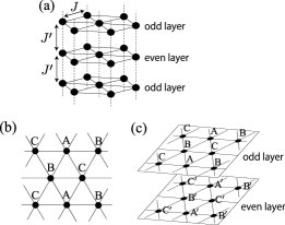
Figure 1: (a) Weakly-coupled layers of triangular lattice. (b) A three-sublattice spin structure expected on a triangular lattice. The spins on the sites with the same letter points in the same direction. (c) A six-sublattice spin structure on a layered triangular lattice.

The Hamiltonian of the Heisenberg model on layers of triangular lattice [see Fig. 1(a)] is given by

$$\hat{\mathcal{H}}=J\sum_{\langle i,j\rangle}\hat{\bm{S}}_{i}\cdot\hat{\bm{S}}_{j}+J^{\prime}\sum_{\langle i,l\rangle^{\prime}}\hat{\bm{S}}_{i}\cdot\hat{\bm{S}}_{l}-H\sum_{i}\hat{S}^{z}_{i},$$ (1)

where both the intralayer ($J$) and interlayer ($J^{\prime}$) nearest-neighbor (NN) couplings are assumed to be antiferromagnetic. We investigate the $S=1/2$ case that exhibits the strongest quantum fluctuations.

For a single layer of triangular lattice (or $J^{\prime}=0$), the ground-state spin configuration usually forms a three-sublattice structure as shown in Fig. 1(b) as long as the system only has spatially isotropic NN interactions. However, real TLAF compounds such as Ba₃CoSb₂O₉ have a quasi-2D structure that consists of magnetic triangular-lattice layers separated from each other by a nonmagnetic layer shirata-12 . Therefore, one has to consider a small but finite interlayer interaction $J^{\prime}$ between spins on different layers. For a ferromagnetic $J^{\prime}<0$, it is expected that the spins along the stacking direction tend to point in the same direction and the three-sublattice spin configuration on each layer is more stabilized. A quite small $|J^{\prime}|\ll J$ can be thus negligible when the magnetic layers are well separated. However, we will show that when $J^{\prime}>0$, even a small interlayer interaction could play an essential role in determining the ground-state spin configuration of TLAFs under magnetic field. The consideration of this effect due to weak three dimensionality is a key to quantitatively describe quasi-2D quantum TLAF compounds with a microscopic model Hamiltonian.

III Cluster Mean-Field Approach with Cluster-Size Scaling for Quantum Spins

The classical counterpart of the model (1) is written in terms of three-dimensional vector $\bm{S}_{i}$ with a fixed length $|\bm{S}_{i}|=1/2$ instead of quantum spin-1/2 operator $\hat{\bm{S}}_{i}$. It is known that the ground state of the classical Heisenberg model on a 2D triangular lattice ($J^{\prime}=0$) cannot be uniquely determined under magnetic field ($H\neq 0$) kawamura-85 ; capriotti-98 . Although the classical-spin angles on the three-sublattice structure shown in Fig. 1(a) have six degrees of freedom, the minimization of the classical energy only gives the constraint $\bm{S}_{A}+\bm{S}_{B}+\bm{S}_{C}=(0,0,H/3J)$ for $0<H<H_{s}$ kawamura-85 ; capriotti-98 . Here, $H_{s}=9J/2$ is the saturation field, above which all the spins are aligned parallel to the magnetic field. Except the trivial degeneracy from the $U(1)$ symmetry, there still remain two degrees of freedom. Therefore, spin configurations in the ground-state magnetization process ($0<H<H_{s}$) are continuously degenerate. The total magnetization per site, $M\equiv\sum_{i}S_{i}^{z}/N$ with $N$ being the number of lattice sites, is given by $H/9J$ as a linear function of the magnetic field strength for any magnetization process in the degenerate manifold.

In the quantum spin-1/2 system, however, the classical degeneracy is lifted by quantum fluctuation effects. For TLAFs, it is now established that the sequence of the “Y,” up-up-down, and 0-coplanar states [Fig. 2] is selected as the lowest-energy magnetization process chubukov-91 ; nishimori-86 ; honecker-04 ; yoshikawa-04 ; farnell-09 ; sakai-11 . The magnetization curve $M(H)$ is no longer a linear function of $H$, and exhibits a magnetization plateau at one-third of the saturation magnetization reflecting the stabilization of the up-up-down state over a finite range of magnetic field strength.

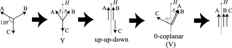
Figure 2: The ground-state magnetization process of quantum Heisenberg antiferromagnets on a purely 2D triangular lattice. Each arrow represents the spin angle on the sublattice A, B, or C. The 0-coplanar state is also called the “V” state.

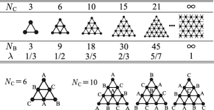
Figure 3: Series of clusters used in the present CMF+S study. The lower illustrations show the independent clusters that have to be considered under the three-sublattice ansatz in the purely 2D case. The cluster of $N_{C}=3$, 15, or 21 is similar to that of $N_{C}=6$.

We employ here the CMF+S method yamamoto-14 ; yamamoto-12-1 ; yamamoto-12-2 ; yamamoto-13-2 ; morenocardone-14 to take into account the quantum effects and interlayer coupling. In general, the number of spins that can be numerically diagonalized on current computer resources is very limited. To avoid strong finite-size effects in such exact diagonalization on small clusters, we impose a self-consistent mean-field boundary condition instead of the usual periodic or open one. First, we approximate the Hamiltonian $\hat{\mathcal{H}}$ on $N$ sites ($N\rightarrow\infty$ in the thermodynamic limit) by the sum of $N/N_{C}$ cluster Hamiltonians on a cluster of $N_{C}$ sites. The inter-cluster interactions are decoupled as $\hat{S}_{i}^{\alpha}\hat{S}_{j}^{\alpha}\rightarrow\langle\hat{S}_{i}^{\alpha}\rangle\hat{S}_{j}^{\alpha}+\langle\hat{S}_{j}^{\alpha}\rangle\hat{S}_{i}^{\alpha}$ ($\alpha=\{x,y,z\}$). Thus, the cluster Hamiltonian $\hat{\mathcal{H}}_{C_{n}}$ includes the expectation values $\langle\hat{S}_{i}^{\alpha}\rangle$ as mean fields to be determined self-consistently. The sublattice magnetic moment $m^{\alpha}_{\mu}$ on sublattice $\mu$ is given by

$$m^{\alpha}_{\mu}=\frac{1}{N_{\mu}}\sum_{n}\sum_{i_{\mu}\in C_{n}}{\rm Tr}\left(\hat{S}_{i_{\mu}}^{\alpha}e^{-\beta\hat{\mathcal{H}}_{C_{n}}}\right)\Big{/}{\rm Tr}(e^{-\beta\hat{\mathcal{H}}_{C_{n}}}),$$ (2)

where $n=1,2,\cdots,M_{C}$ with $M_{C}$ being the number of the independent clusters (specifically given later), $N_{\mu}$ is the number of total sites belonging to the sublattice $\mu$ in the $M_{C}$ clusters, and $\beta=1/T$ (we take $T\rightarrow 0$ in the present study). Substituting $m^{\alpha}_{\mu}$ into $\langle\hat{S}_{i_{\mu}}^{\alpha}\rangle$ in $\hat{\mathcal{H}}_{C_{n}}$, Eq. (2) becomes a set of self-consistent equations for $m^{\alpha}_{\mu}$.

Usually, one gets some different sets of solutions for $m^{\alpha}_{\mu}$ depending on the initial values in the iteration process to solve the self-consistent equations. The spin configuration of each solution at a given magnetic field strength $H$ is identified by the converged values of $m^{\alpha}_{\mu}$ on each sublattice $\mu$. Since the energy difference between different spin configurations can be estimated by integrating the magnetization curve $M(H)$ (which is given by the average of $m_{\mu}^{z}$ over $\mu$) with respect to $H$ from $H_{s}$, one can determine the ground-state magnetization process by comparing the energies of the different solutions.

To efficiently treat possible spin configurations in quasi-2D TLAFs, we choose a series of triangular-shaped clusters of up to $N_{C}=21$, displayed in Fig. 3. The above-mentioned approach reproduces the classical ground state for $N_{C}=1$, and allows for a systematic inclusion of non-local fluctuations as $N_{C}$ increases. Therefore, we eventually make an extrapolation of the results for different values of $N_{C}$ to the limit of $N_{C}\rightarrow\infty$, where long-range fluctuations in each triangular-lattice layer are fully included. The scaling parameter $\lambda\equiv N_{B}/3N_{C}$ ($N_{B}$ is the number of bonds treated exactly) varies from 0 for $N_{C}=1$ to 1 for $N_{C}=\infty$.

IV Purely Two-Dimensional Case ($J^{\prime}=0$)

We first present the CMF+S result for the magnetization curve of the Heisenberg model on a single layer of triangular lattice ($J^{\prime}=0$) for comparisons with some known results obtained by other theoretical methods chubukov-91 ; honecker-04 ; farnell-09 ; sakai-11 . Under the assumption of the three-sublattice structure shown in Fig. 1(b), the number of independent clusters that have to be treated in the CMF+S self-consistent equations (2) is $M_{C}=1$ for $N_{C}=3$, 6, 15, or 21, while $M_{C}=3$ for $N_{C}=10$ (see the lower illustrations of Fig. 3).

The obtained magnetization curves $M(H)$ for each $N_{C}$ are shown in Fig. 4(a). The quantum fluctuations select the sequence of the Y, up-up-down, and 0-coplanar states as expected. The magnetization curve exhibits the one-third quantum magnetization plateau. As the size of the cluster $N_{C}$ increases, the plateau gets wider, indicating that the effects of quantum fluctuations are properly included. Figure 4(b) shows the critical field strength at each of end points of the plateau (named $H_{c1}$ and $H_{c2}$) as a function of the scaling parameter $\lambda$. We perform a linear extrapolation $N_{C}\rightarrow\infty$ ($\lambda\rightarrow 1$) of the data calculated with the three largest clusters. The extrapolated values are given as $H_{c1}(\infty)/J=1.359$ and $H_{c2}(\infty)/J=2.196$, respectively. These values are somewhat different from the linear-spin-wave result (1.248 and 2.145 chubukov-91 ) and comparable with those obtained by the exact diagonalization with the periodic boundary condition (1.38 and 2.16 honecker-04 ; sakai-11 ) and by the coupled cluster method (1.37 and 2.15 farnell-09 ).

In the previous CMF+S study on the $XXZ$ Hamiltonian yamamoto-14 we derived the phase diagram in the plane of the $XXZ$ anisotropy and magnetic field strength by extrapolating the values of the anisotropy parameter $J/J_{z}$ at each phase boundary with $H/H_{s}$ fixed. Since we took sufficiently many but necessarily a finite number of $H/H_{s}$ values, a further interpolation was needed to obtain the critical fields corresponding to the isotropic Heisenberg model, namely to the line $J/J_{z}=1$. This procedure gave $H_{c1}/J=1.345$ and $H_{c2}/J=2.113$ yamamoto-14 . It is expected that the values obtained by the present work ($1.359$ and $2.196$ respectively) are more accurate for the following two reasons. First, the more direct scaling procedure for the magnetization curve of the Heisenberg model does not require further interpolations. Second, the extrapolation to the infinite-size limit based on the linear fit appears to work even more efficiently for the present treatment (in which the critical $H/H_{s}$ is extrapolated) compared to the $XXZ$ model study (in which the critical $J/J_{z}$ is extrapolated).

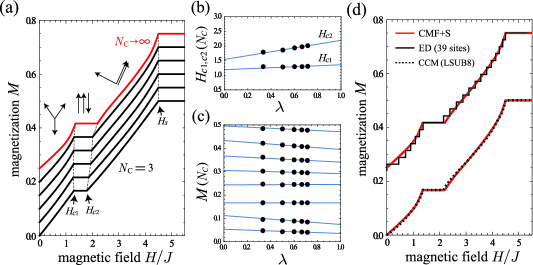
Figure 4: (a) Ground-state magnetization curves of the Heisenberg model on a single layer of triangular lattice for $N_{C}=3$, 6, 10, 15, 21, and $\infty$ (from bottom to top). All the curves apart from the bottom one are vertically shifted by 0.05, 0.1, 0.15, 0.2, 0.25, respectively, for clarity. (b) Cluster-size scalings of the data for the phase transition points $H_{c1}$ and $H_{c2}$. (c) Cluster-size scalings of the data for the magnetization $M$ at the rescaled field strength $H^{\prime}=0.4$ and 0.8 (lower two lines), at $H_{c1}\leq H^{\prime}\leq H_{c2}$ (the line of $M=1/6$), and at $H^{\prime}=2.8$, 3.2, 3.6, 4.0, and 4.4 (upper five lines). (d) Comparisons with the exact diagonalization (ED) with the periodic boundary condition sakai-11 and with the coupled cluster method (CCM) farnell-09 . The upper curves are vertically shifted by 0.25 for clarity.

In order to make cluster-size scaling of the entire magnetization curve $M(H)$, first we have to change the scale of each curve obtained with finite $N_{C}$ with respect to $H$ as $H\rightarrow H^{\prime}$ with

$$H^{\prime} = \frac{H_{c1}(\infty)}{H_{c1}(N_{C})}H~{}~{}{\rm for}~{}~{}0\leq H\leq H_{c1}(N_{C}),$$

$$H^{\prime} = \frac{H_{c2}(\infty)-H_{c1}(\infty)}{H_{c2}(N_{C})-H_{c1}(N_{C})}\big{(}H-H_{c1}(N_{C})\big{)}+H_{c1}(\infty)$$

$$~{}~{}{\rm for}~{}~{}H_{c1}(N_{C})\leq H\leq H_{c2}(N_{C}),$$

and

$$H^{\prime} = \frac{H_{s}-H_{c2}(\infty)}{H_{s}-H_{c2}(N_{C})}\big{(}H-H_{c2}(N_{C})\big{)}+H_{c2}(\infty)$$

$$~{}~{}{\rm for}~{}~{}H_{c2}(N_{C})\leq H\leq H_{s}$$

so that the phase boundaries for all finite $N_{C}$ have the same location as those of the limit $N_{C}\rightarrow\infty$ ($H_{c1}(\infty)$ and $H_{c2}(\infty)$) yamamoto-15 . The extrapolation of the magnetization $M$ at different values of the rescaled $H^{\prime}$ are shown in Fig. 4(c). The top curve in Fig. 4(a) is the obtained CMF+S magnetization curve, which is compared with the other numerical results sakai-11 ; farnell-09 in Fig. 4(d). We can see an excellent agreement of the CMF+S curve with the data extracted from Refs. sakai-11, and farnell-09, , regarding the locations of the phase transition points and the nonlinear bending due to the quantum effects.

V The Role of Weak Interlayer Coupling ($J^{\prime}\neq 0$)

Weak three-dimensionality is not avoidable in real quasi-2D TLAF compounds. Since there are numerous nearly-degenerate states in frustrated systems, even very small interlayer interaction can compete with quantum fluctuations and affect the ground-state selection. In the previous study yamamoto-15 , while effects of the interlayer coupling have been discussed with a focus on the case where easy-plane exchange anisotropy exists, we have not explained the detailed magnetization process for the isotropic case. Therefore, here let us discuss the role of interlayer coupling $J^{\prime}$ on the magnetization process of the fundamental Heisenberg model (1) in a quantitative way with the use of the CMF+S.

For weakly-coupled triangular-lattice layers, we assume the six sublattice structure shown in Fig. 1(c) ($\mu=$A, B, C, A^′, B^′, or C^′) susuki-13 . The number of independent clusters that have to be considered in the CMF+S is now $M_{C}=2$ for $N_{C}=3$, 6, 15, or 21, while $M_{C}=6$ for $N_{C}=10$. The saturation field is given by $H_{s}=9J/2+2J^{\prime}$.

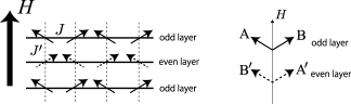
Figure 5: Typical spin stacking pattern in weakly-coupled antiferromagnetic layers of bipartite lattice under magnetic field. The right panel is the corresponding schematic illustration.

In general, when the interlayer interaction is antiferromagnetic ($J^{\prime}>0$), antiparallel spin alignment is favored along the stacking direction. If each layer consists of a bipartite lattice, it is expected that the in-plane magnetic order is just stacked alternately as shown in Fig. 5. However, for non-bipartite lattices such as the triangular lattice, the in-plane three-sublattice magnetic order could compete with the demand of antiparallel alignment along the stacking direction. As a result of the incompatibility, the lowest-energy stacking pattern can be changed depending on the magnetic field strength as will be shown below.

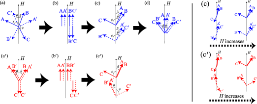
Figure 6: Two candidate magnetization processes of quasi-2D Heisenberg TLAFs. The interlayer interaction $J^{\prime}$ acts on the NN bonds between A and A^′, between B and B^′, and between C and C^′. The right panels show the changes of relative angles $\theta$, $\phi$, and $\chi$ in the states (c) and (c^′) as $H$ increases.

For TLAFs in the presence of antiferromagnetic interlayer coupling, we found two candidate magnetization processes as solutions of Eq. (2) yamamoto-15 , both of which reduce to the sequence of the Y, up-up-down, and 0-coplanar states at the purely 2D limit. Figure 6 shows the two branches (a)-(b)-(c)-(d) and (a^′)-(b^′)-(c^′). From comparison between (a) and (a^′) or between (b) and (b^′), it is obviously seen that the former process has a lower energy for low magnetic fields since $J^{\prime}>0$ favors antiparallel alignment on interlayer bonds. However, the magnitude relation between the energies of (c) and (c^′) at strong fields can be reversed as $H$ increases. Note that the relative angles ($\theta$, $\phi$, and $\chi$) among the six sublattice magnetic moments are gradually changed as a function of $H$ even in the same phase. As can be seen in the right panels of Fig. 6, when the spins are almost collinear, the energy of (c^′) should be higher than that of (c) due to the high interlayer bond energy of field-parallel spin components. However, when the magnetic field is further increased, the (c^′) configuration becomes advantageous against (c) since it can reduce more interlayer bond energy of field-transverse components. As a result, a field-induced first-order transition between (c) and (c^′) is expected to occur at a certain strong magnetic field.

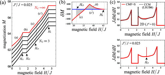
Figure 7: (a) Ground-state magnetization curves of the Heisenberg model on weakly-coupled layers of triangular lattice for $N_{C}=3$, 6, 10, 15, 21, and $\infty$ (from bottom to top). We set $J^{\prime}=0.025J$. All the curves apart from the bottom one are vertically shifted by 0.05, 0.1, 0.15, 0.2, 0.25, respectively, for clarity. (b) The high-field part of the magnetization curves of the two branches. Here, $\delta M$ is the magnetization measured from that of the branch (a^′)-(b^′)-(c^′). The critical field strength $H_{c3}$ is determined so that the areas of the shaded regions are equal. The result for $N_{C}=21$ is shown. (c) The CMF+S result ($N_{C}\rightarrow\infty$) of the susceptibility $JdM/dH$ for $J^{\prime}=0$ (upper) and $J^{\prime}=0.025J$ (lower). The susceptibility of a single layer of triangular lattice ($J^{\prime}=0$) is compared with that of the CCM farnell-09 .

Figure 7(a) shows the ground-state magnetization process obtained by solving Eq. (2) for different $N_{C}$ in the case of a very small interlayer interaction $J^{\prime}=0.025J$. Indeed, an extra discontinuous phase transition that was not seen in the purely 2D case is found at a strong field, although the discontinuity in $M$ is quite small. The transition point $H_{c3}$ can be determined by Maxwell’s construction for the difference of the curves $M(H)$ in the two magnetization processes [see Fig. 7(b)]. Thus, it is concluded that the magnetization process is given by (a)-(b)-(c)-(c^′) for quasi-2D TLAFs.

Performing a cluster-size extrapolation ($N_{C}\rightarrow\infty$) in a similar way to the purely 2D case, we obtain the CMF+S result of the magnetization curve [the top curve in Fig. 7(a)]. Since $J^{\prime}$ is assumed here to be very small, the general behavior of the curve differs little from that of the purely 2D case. However, as shown in Fig. 7(c), the existence of the additional quantum first-order transition is clearly seen in the field derivative of $M(H)$ as the divergence at $H=H_{c3}\approx 0.712H_{s}$, in contrast to the purely 2D ($J^{\prime}=0$) case.

VI Summary

In summary, we have studied the magnetization process of the spin-1/2 Heisenberg model on layered triangular lattice with and without weak interlayer coupling. Our numerical calculations with the CMF+S method properly described the one-third magnetization plateau expected in quantum TLAFs and provided a quantitative agreement with the numerical data of the ED honecker-04 ; sakai-11 and the CCM farnell-09 for a single layer of triangular lattice. Moreover, we discussed the detailed magnetization process in the presence of weak interlayer coupling, which is unavoidable in real quasi-2D compounds. We presented the magnetization and susceptibility curves of the isotropic Heisenberg model, which was not reported in our previous study yamamoto-15 . Although a small interlayer coupling does not change the apparent shape of the magnetization curve, an additional first-order phase transition occurs at $H\approx 0.712H_{s}$ above the one-third plateau. This extra transition is visible as a small discontinuous jump in the magnetization curve and a divergence in the susceptibility. From a comparison of the present isotropic Heisenberg model with the previous easy-plane case yamamoto-15 , the easy-plane anisotropy seems not to be relevant for the qualitative feature of the magnetization process and the shape of the magnetization curve including the extra first-order transition as long as the magnetic field is applied in the direction parallel to the easy plane. Since the appearance of the high-field first-order transition stems from the incompatibility between the in-plane quantum magnetic order and the demand of antiparallel alignment along the stacking direction, a similar magnetization process is expected to be obtained for larger spins, e.g., $S=1$ and $S=3/2$.

Here, we discussed the case of weak interlayer coupling ($J^{\prime}=0.025J$) employing the CMF+S based on 2D clusters shown in Fig. 3. For larger values of $J^{\prime}$ ($\gtrsim 0.2J$), it has been predicted for the Heisenberg model that the umbrella state is stabilized at strong fields nikuni-95 ; marmorini-15 . Therefore, for moderate interlayer couplings, the magnetization process should become more complex due to the competition of the umbrella state and the coplanar states shown in Fig. 6. It remains an interesting open problem.

We acknowledge Hidekazu Tanaka and Yoshitomo Kamiya for useful discussions. This work was supported by KAKENHI Grants from JSPS No. 25800228 (I.D.), No. 25220711 (I.D.), and No. 26800200 (D.Y.).

References

- (1) O. A. Starykh, Reports on Progress in Physics 78, 052502 (2015) and references therein.
- (2) Y. Shirata, H. Tanaka, A. Matsuo, and K. Kindo, Phys. Rev. Lett. 108, 057205 (2012).
- (3) H. D. Zhou, C. Xu, A. M. Hallas, H. J. Silverstein, C. R. Wiebe, I. Umegaki, J. Q. Yan, T. P. Murphy, J.-H. Park, Y. Qiu, J. R. D. Copley, J. S. Gardner, and Y. Takano, Phys. Rev. Lett. 109, 267206 (2012).
- (4) T. Susuki, N. Kurita, T. Tanaka, H. Nojiri, A. Matsuo, K. Kindo, and H. Tanaka, Phys. Rev. Lett. 110, 267201 (2013).
- (5) G. Koutroulakis, T. Zhou, Y. Kamiya, J. D. Thompson, H. D. Zhou, C. D. Batista, and S. E. Brown, Phys. Rev. B 91, 024410 (2015).
- (6) G. Quirion, M. Lapointe-Major, M. Poirier, J. A. Quilliam, Z. L. Dun, and H. D. Zhou, Phys. Rev. B 92, 014414 (2015).
- (7) J. Ma, Y. Kamiya, T. Hong, H. B. Cao, G. Ehlers, W. Tian, C. D. Batista, Z. L. Dun, H. D. Zhou, and M. Matsuda, arXiv:1507.05702
- (8) M. Lee, J. Hwang, E. S. Choi, J. Ma, C. R. Dela Cruz, M. Zhu, X. Ke, Z. L. Dun, and H. D. Zhou, Phys. Rev. B 89, 104420 (2014).
- (9) K. Yokota, N. Kurita, and H. Tanaka, Phys. Rev. B 90, 014403 (2014).
- (10) Y. C. Sun, Z. W. Ouyang, M. Y. Ruan, Y. M. Guo, J. J. Cheng, Z. M. Tian, Z. C. Xia, and G. H. Rao, J. Magn. Magn. Mater. 393, 273 (2015).
- (11) T. Ono, H. Tanaka, H. Aruga Katori, F. Ishikawa, H. Mitamura, and T. Goto, Phys. Rev. B 67, 104431 (2003).
- (12) N. A. Fortune, S. T. Hannahs, Y. Yoshida, T. E. Sherline, T. Ono, H. Tanaka, and Y. Takano, Phys. Rev. Lett. 102, 257201 (2009).
- (13) A. V. Chubukov and D. I. Golosov, J. Phys.: Condens. Matter 3, 69 (1991).
- (14) H. Nishimori and S. Miyashita, J. Phys. Soc. Jpn. 55, 4448 (1986).
- (15) A. Honecker, J. Schulenburg, and J. Richter, J. Phys. Condens. Matter 16, S749 (2004).
- (16) S. Yoshikawa, K. Okunishi, M. Senda, and S. Miyashita, J. Phys. Soc. Jpn. 73, 1798 (2004).
- (17) D. J. J. Farnell, R. Zinke, J. Schulenburg, and J. Richter, J. Phys. Condens. Matter 21, 406002 (2009).
- (18) T. Sakai and H. Nakano, Phys. Rev. B 83, 100405(R) (2011).
- (19) O. Götzea, J. Richtera, R. Zinkeb, and D. J. J. Farnell, Journal of Magn. Magn. Mater. 397, 333 (2016).
- (20) V. S. Maryasin and M. E. Zhitomirsky, Phys. Rev. Lett. 111, 247201 (2013).
- (21) D. Yamamoto, G. Marmorini, and I. Danshita, Phys. Rev. Lett. 114, 027201 (2015).
- (22) D. Sellmann, X.-F. Zhang, and S. Eggert, Phys. Rev. B 91, 081104 (2015).
- (23) D. Yamamoto, I. Danshita, and C. A. R. Sá de Melo, Phys. Rev. A 85, 021601(R) (2012).
- (24) D. Yamamoto, A. Masaki, and I. Danshita, Phys. Rev. B 86, 054516 (2012).
- (25) D. Yamamoto, T. Ozaki, C. A. R. Sá de Melo, and I. Danshita, Phys. Rev. A 88, 033624 (2013).
- (26) D. Yamamoto, G. Marmorini, and I. Danshita, Phys. Rev. Lett. 112, 127203 (2014); ibid, 112, 259901 (2014).
- (27) M. Moreno-Cardoner, H. Perrin, S. Paganelli, G. De Chiara, and A. Sanpera, Phys. Rev. B 90, 144409 (2014).
- (28) H. Kawamura and S. Miyashita, J. Phys. Soc. Jpn. 54, 4530 (1985).
- (29) L. Capriotti, R. Vaia, A. Cuccoli, and V. Tognetti, Phys. Rev. B 58, 273 (1998).
- (30) T. Nikuni and H. Shiba, J. Phys. Soc. Jpn. 64, 3471 (1995).
- (31) G. Marmorini, D. Yamamoto, and I. Danshita (in preparation).