Boundary conditions for the solution of the 3-dimensional Poisson equation in open metallic enclosures

Abstract

Numerical solution of the Poisson equation in metallic enclosures, open at one or more ends, is important in many practical situations such as High Power Microwave (HPM) or photo-cathode devices. It requires imposition of a suitable boundary condition at the open end. In this paper, methods for solving the Poisson equation are investigated for various charge densities and aspect ratios of the open ends. It is found that a mixture of second order and third order local asymptotic boundary condition (ABC) is best suited for large aspect ratios while a proposed non-local matching method, based on the solution of the Laplace equation, scores well when the aspect ratio is near unity for all charge density variations, including ones where the centre of charge is close to an open end or the charge density is non-localized. The two methods complement each other and can be used in electrostatic calculations where the computational domain needs to be terminated at the open boundaries of the metallic enclosure.

I Introduction

Open computational boundaries pose a challenge for both time-dependent and time-independent problems in fields as diverse as electromagnetics, quantum mechanics, fluid dynamics and biological systems. In electromagnetics, examples of devices with one or more open ends include the Virtual Cathode Oscillator or the Klystron granat ; cairns , those involving photo-cathodes or a charge-particle beam in a conducting pipe. Their simulation using a Particle-in-Cell (PIC) code requires the imposition of artificial boundary conditions at the open ends of the computational domain. For time-varying electromagnetic fields, the Perfectly Matched Layer (PML) technique is commonly adopted and provides a viable non-reflecting termination of the computational domain at an extra cost berenger ; taflove . For electrostatic fields, the Poisson equation

$$\nabla^{2}V({\bf r})=-\rho({\bf r})/\epsilon_{0}$$ (1)

needs to be solved with specified boundary conditions and for open ends, special techniques need to be adopted konrad . Here $V$ is the electrostatic potential, $\rho$ is the charge density and $\epsilon_{0}$ is free space permittivity.

Depending on the physical situation being modeled, various scenarios may arise. When the problem of interest comprises of a charge distribution that is sufficiently isolated from other objects, the boundary condition at infinity can be implemented by choosing the computational domain to be spherical and applying a suitable artificial boundary condition at the surface. Alternately, the free-space Green’s function can be used to evaluate the field inside the computational domain. In such situations, efficient methods exist that limit the computational cost isf .

Quite often, in addition to charges, the computational domain may consist of metallic objects where additional boundary conditions need to be imposed. When the electrostatic field outside the metallic objects is of interest, the computational boundary can be a chosen to be sphere or a cube with a suitable artificial boundary condition. The local Asymptotic Boundary Conditions (ABC) bayliss ; mittra , the Dirichlet to Neumann (DtN) map han ; keller and hybrid methods such as the boundary relaxation/potential method silvester ; Miller ; zwang and the boundary integral method bim are particularly useful in such situations.

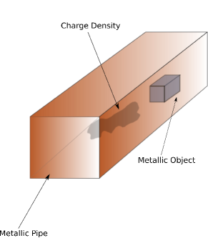
Figure 1: A schematic of an open pipe having charges and a metallic structure inside.

Finally, the region of interest may lie inside open metallic objects such as a guide tube or an open pipe (see Fig 1) enclosing charges and perhaps other metallic structures such as a cathode or anode. In such cases, in order to minimize computational resources, it is natural to limit the computational domain to the extent of the outer open metallic enclosure and impose a suitable approximate boundary condition at the open surfaces (such as the two ends of a pipe or guide tube). We shall limit ourselves to this last category of problems in this paper.

To the best of our knowledge, there are few boundary conditions available in open literature that can be directly applied in a finite difference scheme when the computational domain is truncated at one or more open ends. The simplest of these is the first order Asymptotic Boundary Condition (ABC1),

$$\frac{\partial V}{\partial r}+\frac{V}{r}=0$$ (2)

which can be easily implemented at an open boundary $x_{i}=$ constant, thereby allowing a solution on a Cartesian grid using the finite difference technique. ABC1 is based on the general solution jackson

$$V(r,\theta,\phi)=\sum_{l=0}^{\infty}\sum_{m=-l}^{m=l}\frac{B_{lm}}{r^{l+1}}Y_{l,m}(\theta,\phi)$$ (3)

in the charge-free region outside the computational domain. Here $Y_{l,m}(\theta,\phi)$ are the spherical harmonics and $B_{lm}$ are unknown coefficients. Equation (2) follows on noting that

$$\frac{\partial V}{\partial r}+\frac{V}{r}=\mathcal{O}(1/r^{3})$$ (4)

and, as a first approximation, the right hand side can be set to zero. Successive boundary conditions can be similarly derived bayliss ; mittra . For example, the second order asymptotic boundary condition (ABC2) is

$$\frac{\partial^{2}V}{\partial r^{2}}+\frac{4}{r}\frac{\partial V}{\partial r}+\frac{2V}{r^{2}}=\mathcal{O}(1/r^{5})\simeq 0.$$ (5)

In general, there exists a hierarchy of such boundary conditions which can be expressed as

$$\prod_{j=1}^{n}({\partial\over\partial r}+{(2j-1)\over r})V=0$$ (6)

which represent the $n^{th}$ order asymptotic boundary condition, ABCn. A local implementation however requires the use of lower order ABC, thereby diluting the accuracy. For example, a local implementation of the second order method (ABC2) requires the use of ABC1 in order to compute mixed derivatives $\partial^{2}V/\partial x_{i}\partial x_{j}$ at an open boundary $x_{i}=$ constant. We shall show that ABC2 generally delivers good results unless the charge density variation perpendicular to the open boundary is low, in which case the method is found to be inappropriate. For large aspect ratio open boundaries however, the Asymptotic Boundary Condition remains stable and consistent and as we shall show, a mixture of ABC2 and ABC3 can help reduce errors.

Apart from the local asymptotic boundary conditions, non-local hybrid methods can be applied to an open pipe geometry even though they are resource intensive. The boundary relaxation/potential technique for solving the Poisson equation relies on iteratively correcting a solution of the Poisson equation with an assumed potential at the open boundary.

Both the asymptotic boundary condition (ABC) and the boundary potential method can be directly implemented in an open pipe or guide-tube geometry without expanding the computational domain. We propose here an alternate non-local method (referred to as Method-1 hereafter) that complements ABC when the aspect ratio of the open surface is near unity. It scores very well over ABC when the centre of charge is near an open end or when the charge distribution is non-localized. It relies on matching the potential to the solution of the Laplace equation at the open boundary using $(l_{max}+1)^{2}$ points where the sum over $l$ in Eq. (3) is restricted to $l_{max}$. In effect it uses less than $0.5\%$ points on the open surface and gives consistent results that are generally better than the methods discussed above. It has been studied using Finite Element Method (FEM) chari1 ; chari2 but its application using Finite Difference is limited to a 2-dimensional situation hammel perhaps on account of convergence issues.

In section II, we outline the proposed Method-1 that we shall adopt for aspect ratios close to unity. Thereafter, we shall review the implementation of the second and third order Asymptotic Boundary Conditions (ABC2 and ABC3) in section III and outline the boundary potential method in section IV for the sake of comparison. Section V deals with the numerical results for charge densities in an open rectangular pipe, a problem for which, the exact solution is known.

II Non-local Boundary truncation using Laplace solution (Method-1)

We propose here a method that is especially useful when the aspect ratio of the open end is near unity and charges are near the open boundary.

Consider an open boundary $x=x_{N}$ in a 3-dimensional Cartesian grid where $x_{1},x_{2},\ldots,x_{N}$ are equispaced points along the $X-$axis. We need to specify the boundary potential $V_{N,j,k}$ at the open boundary $x=x_{N}$ in order to solve the Poisson equation inside the computational domain. In this section, we determine a boundary truncation scheme whereby $\{V_{N,j,k}\}$ can be expressed in terms of $\{V_{N-1,j,k}\}$. A self-consistent iteration scheme can then be used to find the potential in the region of interest.

Using central difference, the normal derivative of the potential at the open boundary is

$${\frac{\partial V}{\partial x}}|_{x=x_{N}}=\frac{(V_{N+1,j,k}-V_{N-1,j,k})}{2h_{x}}$$ (7)

where $h_{x}$ is the spacing between points along the $X$-direction (similarly, $h_{y}$ and $h_{z}$ denote spacing along $Y$ and $Z$ directions). Using the Laplace solution (Eq. 3) to evaluate $(\partial V/\partial x)_{|_{x=x_{N}}}$, and $V_{N+1,j,k}$, a system of linear equations can be set up to determine the unknown coefficients $B_{lm}$ in terms of $V_{N-1,j,k}$. To this end, note that

$$\frac{\partial V}{\partial x} = \sum_{l=0}^{\infty}\sum_{m=-l}^{l}B_{lm}\left[-\frac{(l+1)x}{r^{l+3}}Y_{l,m}(\theta,\phi)~{}\right.$$ (8)

$$+ \left.\frac{1}{r^{l+1}}\left\{\frac{\partial Y_{l,m}}{\partial\theta}\frac{\partial\theta}{\partial x}+\frac{\partial Y_{l,m}}{\partial\phi}\frac{\partial\phi}{\partial x}\right\}\right]$$

where

$$\frac{\partial\theta}{\partial x} = \frac{zx}{r^{2}\sqrt{x^{2}+y^{2}}}$$ (9)

$$\frac{\partial\phi}{\partial x} = -\frac{y}{x^{2}+y^{2}}$$ (10)

and

$$\frac{\partial Y_{l,m}}{\partial\phi} = \iota mY_{l,m}(\theta,\phi)$$ (11)

$$\frac{\partial Y_{l,m}}{\partial\theta} = \sqrt{(l-m)(l+m+1)}~{}e^{-\iota\phi}Y_{l,m+1}(\theta,\phi)$$ (12)

$$+ m\cot\theta~{}Y_{l,m}(\theta,\phi).$$

Here, ($r,\theta,\phi)$ are the spherical polar co-ordinates. Using the above, the system of equations can thus be expressed as

$$\begin{split}\sum_{l=0}^{\infty}\sum_{m=-l}^{l}&B_{lm}\left[\frac{Y_{l,m}(\theta_{N+1},\phi_{N+1})}{r_{N+1}^{(l+1)}}-2h_{x}\left\{-\frac{(l+1)}{r_{N}^{l+3}}x_{N}Y_{l,m}(\theta_{N},\phi_{N})~{}+~{}\right.\right.\\ &\left.\left.\frac{1}{r_{N}^{l+1}}\left(\frac{\partial Y_{l,m}}{\partial\theta}\frac{\partial\theta_{N}}{\partial x}+\frac{\partial Y_{l,m}}{\partial\phi}\frac{\partial\phi_{N}}{\partial x}\right)_{|_{(r_{N},\theta_{N},\phi_{N})}}\right\}\right]=V_{N-1,j,k}\end{split}$$ (13)

In practice, the sum over $l$ must be truncated at $l=l_{max}$ and the number of points $\{j,k\}$ on the open boundary $x=x_{N}$ chosen to equal the number of unknown coefficients $B_{lm}$. It is easy to verify that truncation at $l=l_{max}$ leads to $N_{max}=(l_{max}+1)^{2}$ number of unknowns. Thus $N_{max}$ points must be chosen appropriately on the open boundary.

The system of equations in Eq. (13) can be solved to yield $B_{lm}$ which in turn can be used to find the potential $\{V_{N,j,k}\}$ in terms of $\{V_{N-1,j,k}\}$. Similarly, for a boundary on the left ($x=x_{1}$), $\{V_{1,j,k}\}$ can be expressed in terms of $\{V_{2,j,k}\}$. Thus, the potential at all points between $x_{1}$ and $x_{N}$ can be updated using a standard Poisson solver.

The numerical results using Method-1 are presented in section V. In the finite difference implementation however, there are convergence issues depending on origin. Nevertheless, the domain of convergence can be determined easily when the aspect ratio of the open face is between $1/4$ and $4$.

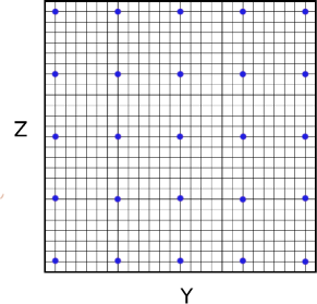
Figure 2: A $27\times 27$ grid on open surface $X=$constant along with the 25 points (solid dots) chosen for matching the solution. In the rest of the paper, a $41\times 41$ grid is used.

Importantly, for most problems, $l_{max}=4$ is sufficient for implementing the open boundary. Thus a total of 25 points on an open surface need to be chosen out of $\mathcal{N}^{2}$ points where $\mathcal{N}$ is the average number of points along the edge of an open face needed by the Poisson solver. We choose an implementation shown in Fig (2).

III Implementation of the Asymptotic Boundary Conditions (ABC)

We shall briefly outline the implementation of the well known Asymptotic Boundary Condition in this section. We shall assume the open face to be $x=$ constant without any loss of generality.

III.1 ABC1

The first order asymptotic boundary condition

$$({\partial\over\partial r}+{1\over r})V=0$$ (14)

can be expressed as

$$V_{x}{\partial x\over\partial r}+V_{y}{\partial y\over\partial r}+V_{z}{\partial z\over\partial r}+{V\over r}=0.$$ (15)

Using $\partial x/\partial r=x/r$, $\partial y/\partial r=y/r$ and $\partial z/\partial r=z/r$, the above equation can be expressed as

$$V_{x}=-{V\over x}-{y\over x}V_{y}-{z\over x}V_{z}$$ (16)

which can be discretized at $x=x_{N-1}$ to yield

$$V_{N}=V_{N-2}-(2h_{x})\left[{V\over x}+{y\over x}V_{y}+{z\over x}V_{z}\right]_{N-1}$$ (17)

where $x_{N}-x_{N-1}=x_{N-1}-x_{N-2}=h_{x}$. Thus the potential at the face $x=x_{N}$ can be expressed in terms of the potential and its derivative inside the computational domain.

III.2 ABC2

The second order asymptotic boundary condition

$${\partial^{2}V\over\partial r^{2}}+{4\over r}{\partial V\over\partial r}+{2V\over r^{2}}=0$$ (18)

can be similarly implemented at an open surface at $x=x_{N}$ on expressing ${\partial^{2}V/\partial r^{2}}$ as

$$V_{rr}=V_{xx}{x^{2}\over r^{2}}+V_{yy}{y^{2}\over r^{2}}+V_{zz}{z^{2}\over r^{2}}+V_{xy}{2xy\over r^{2}}+V_{xz}{2xz\over r^{2}}+V_{yz}{2yz\over r^{2}}.$$ (19)

Thus,

$$V_{x}+{x\over 4}V_{xx}=-{V\over 2x}+{y^{2}\over 4x}V_{yy}+{z^{2}\over 4x}V_{zz}+{yz\over 2x}V_{yz}$$ (20)

so that on discretizing at $x=x_{N-1}$, we have

$$V_{N}=\frac{1}{1+\frac{x}{2h_{x}}}\left[V_{N-2}+\frac{x}{2h_{x}}\left(2V_{N-1}-V_{N-2}\right)\right]+2h_{x}\left[-{V\over 2x}+{y^{2}\over 4x}V_{yy}+{z^{2}\over 4x}V_{zz}+{yz\over 2x}V_{yz}\right]_{N-1}$$ (21)

where $[\ldots]_{N-1}$ denotes discretization at $x=x_{N-1}$.

III.3 ABC3

Implementation of the third order asymptotic boundary condition

$${\partial^{3}V\over\partial r^{3}}+{9\over r}{\partial^{2}V\over\partial r^{2}}+{18\over r^{2}}{\partial V\over\partial r}+{6V\over r^{3}}=0$$ (22)

at the $x=x_{N}$ face requires $V_{rrr}$ to be expressed in terms of the partial derivatives in cartesian co-ordinates:

$$\begin{split}V_{rrr}=&V_{xxx}{x^{3}\over r^{3}}+V_{xxy}{3x^{2}y\over r^{3}}+V_{xxz}{3x^{2}z\over r^{3}}+V_{yyy}{y^{3}\over r^{3}}+V_{yyx}{3xy^{2}\over r^{3}}+V_{yyz}{3y^{2}z\over r^{3}}\\ &+V_{zzz}{z^{3}\over r^{3}}+V_{zzx}{3xz^{2}\over r^{3}}+V_{zzy}{3yz^{2}\over r^{3}}+V_{xyz}{6xyz\over r^{3}}.\end{split}$$ (23)

Together with the expressions for $V_{rr}$ and $V_{r}$, $V_{x}$ can be similarly obtained such that $V_{N}$ is expressed in terms of the potential and its derivatives at interior points. The analysis above can be similarly generalized for faces $y,z$=constant.

IV Truncation using the boundary potential method (BPM)

Apart from the proposed Method-1 and the Asymptotic Boundary Conditions, the Boundary Potential Method can also be directly applied when the computational domain is truncated at the open face. We shall review the implementation briefly and use it in the next section for the sake of comparison.

Consider a metallic rectangular wave-guide with two open faces. It may contain some metallic structure (see Fig. (1)) or a charge distribution $\rho({\bf r})$ or both. We need to solve Poisson equation (Eq. (1) with boundary conditions $V=V_{D}|_{S}$, where $V_{D}$ is the specified potential on the metallic surfaces and $V({\bf r})=Q/(4\pi\epsilon_{0}{\bf r})$ as ${\bf r}\rightarrow\infty$. Here $Q$ is the sum of all charges inside the domain (in this case, the open wave-guide) consisting of charge density $\rho$ and also the surface charges present on all surfaces.

To solve this problem, the following steps need to carried out:

1. Poisson equation in the domain of interest is solved with an assumed potential (e.g. $V=0$) at the open boundaries and the specified potential $V_{D}$ on the remaining surfaces using a standard numerical procedure. The solution $V_{0}({\bf r})$ obtained with the assumed boundary potential is clearly different from the desired solution and gives rise to surface charges at the open boundary. The solution can be corrected iteratively as described in following steps.

2. The screening surface charge density $\sigma_{os}$ at the open surfaces is calculated by taking the normal derivative of the potential $V_{0}({\bf r})$

   $$\sigma_{os}=-\epsilon_{0}{\bf n}\cdot\nabla V_{0}({\bf r}).$$ (24)

3. The boundary potential $V^{k}_{os}$ ($k=0$) at open surface due to all the screening charges is calculated using the free space Green’s function:

   $$V^{0}_{os}({\bf r})=-{\frac{1}{\epsilon_{0}}}\int{\int{dS^{\prime}G({\bf r}|{\bf r^{\prime}})\sigma_{os}({\bf r^{\prime}})}}$$ (25)

4. Next, Laplace equation $\nabla^{2}\psi=0$ is solved inside the domain of interest to calculate the correction potential $\psi$. The boundary conditions on $\psi$ are:

   $$\psi=\begin{cases}V^{k}_{os}&\mbox{at open surfaces},\\ 0&\mbox{at all other surfaces.}\end{cases}$$ (26)

5. The calculated correction potential, $\psi$, itself needs correction. This is so because the free space Green’s function is used to calculate $V^{0}_{os}$, in effect ignoring the presence of all the surfaces where potential was already specified. For instance, in case of a metallic pipe, the presence of the wall and inner metallic structures (if any) is ignored.

   In order to include the effect of all surfaces other than the open surfaces, the screening charge is calculated at these inner surfaces using the normal derivative of $\psi$:

   $$\sigma^{k}_{in}=-\epsilon_{0}{\bf n}\cdot\nabla\psi.$$ (27)

6. The correction in boundary potential due to these screening charges is again calculated using the free space Green’s function.

   $$V^{correction}_{os}({\bf r})={\frac{1}{\epsilon_{0}}}\int{\int{dS^{\prime}G({\bf r}|{\bf r^{\prime}})\sigma^{k}_{in}({\bf r^{\prime}})}}$$ (28)

7. Corrected boundary potential is given by

   $$V^{k}_{os}=\omega V^{0}_{os}+\omega V^{correction}_{os}+(1-\omega)V^{k-1}_{os}.$$ (29)

   For $0<\omega<1$, above correction formula assures convergence for any well resolved geometry Miller .

8. One needs to iterate step 4 to step 7 till $V^{k}_{os}$ converges to the required tolerance level. The solution $V$ to equation 1 is given by:

   $$V({\bf r})=V_{0}({\bf r})+\psi({\bf r})$$ (30)

   where $\psi({\bf r})$ is obtained as in step 4 using converged boundary potentials at the open surfaces while $V_{0}({\bf r})$ is calculated in step 1.

The scheme discussed above is implemented using Finite Difference and compared with the proposed Method-1 and ABC2 in the following section.

V Numerical Results

In order to study the efficacy of the three boundary truncation methods under different conditions, we shall study various charge densities inside a rectangular metallic pipe with open ends having specified aspect ratios. For this problem, the exact solution can be easily computed pipe using the exact Green’s function.

For a rectangular pipe of dimension $L_{x}$, $L_{y}$ and $L_{z}$, with open faces at $x=0$ and $x=L_{x}$, the potential can be expressed as pipe

$$\begin{split}V&(x,y,z)=\frac{2}{L_{y}L_{z}\epsilon_{0}}\sum_{n}\sum_{m}\frac{1}{\gamma_{m,n}}\sin(k_{y}y)\sin(k_{z}z)\times\\ &\iiint\limits_{-\infty}^{~{}~{}~{}~{}\infty}e^{-\gamma_{m,n}|x-x^{\prime}|}\sin(k_{y}y^{\prime})\sin(k_{z}z^{\prime})\rho(x^{\prime},y^{\prime},z^{\prime})d^{3}r^{\prime}\end{split}$$ (31)

where $k_{y}=m\pi/L_{y}$, $k_{z}=n\pi/L_{z}$, $\gamma_{m,n}^{2}=\pi^{2}(m^{2}/L_{y}^{2}+n^{2}/L_{z}^{2})$. We now define various problems based on the form of the charge density $\rho(x,y,z)$. Note that Eq. (31) does not hold if there are other metallic objects inside the pipe.

We shall test the boundary conditions essentially in two different scenarios. In the first, we shall allow the aspect ratio of the open faces to be unity but allowing for variation in the length of the enclosure. The second deals with aspect ratios beyond unity. In both cases, mesh-independence studies have been carried out by ensuring that the average relative error (see Eq. (33)) saturates within an acceptable limit as the size of the grid is increased. While, the grid size at which results become mesh-independent depends on the charge density chosen, it is generally found that a grid size of $81\times 81\times 81$ is adequate. All error estimates reported hereafter use this grid size, unless otherwise mentioned.

V.1 Unit Aspect Ratio

We shall first consider the case where the aspect ratio $L_{y}/L_{z}=1$. To begin with we choose $L_{x}=L_{y}=L_{z}=1.0$m with the open ends at $x=0$ and $x=L_{x}$. The potential is computed using (a) the exact expression given in Eq. (31) with the sum truncated appropriately to ensure convergence (b) the Laplace equation based non-local method of section II (referred to as Method-1) with $l_{max}=4$, (c) the iterative Green’s function based Boundary Potential Method with $\omega=0.5$ and (d) the local asymptotic boundary condition ABC2. In each case a $81\times 81\times 81$ grid is chosen that includes the boundary points. Unless, otherwise specified, all distances are measured in metres, the potential in volts and charge density in coulomb per cubic metre.

Density	Method-1		BPM		ABC-2
	(Full)	(Interior)	(Full)	(Interior)	(Full)	(Interior)
Case-1	1.26%	0.54%	17.41%	7.71%	21.31%	15.64%
Case-2	2.01%	0.62%	21.11%	9.06%	1.68%	1.12%
Case-3	1.5%	0.58%	18.85%	8.18%	10.58%	7.89%

Table 1: The average error for the three charge densities Case-1,2 and 3 for an enclosure with $L_{x}=L_{y}=L_{z}=1$ having open faces at $x=0$ and $x=L_{z}$ (a) the full domain excluding only the boundary points and (b) Interior points. For the full domain, the error analysis considers $N=79^{3}$ points. Since distortion is often closest to the boundary, the error for interior domain is computed using $N=67^{3}$ points i.e. leaving 6 additional points along each face of the computational domain.

V.1.1 Uniform density along the pipe axis (Case-1)

(a) Exact

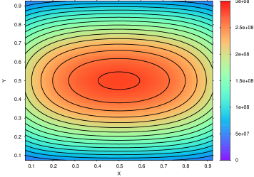
(b) Method-1

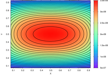
(c) BPM

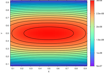
(d) ABC2

Figure 3: The potential $V$ for a charge density uniform in the X-direction and parabolic in the $Y$ and $Z$ directions. A projection on the $XY$ plane $z=0.3$ is shown in each case.

We first choose a charge density that is uniform along the $X$-axis but varies along the $Y$ and $Z$ directions pipe :

$$\rho(x,y,z)=\begin{cases}\left[\frac{L_{y}^{2}}{4}-(y-\frac{L_{y}}{2})^{2}\right]\left[\frac{L_{z}^{2}}{4}-(z-\frac{L_{z}}{2})^{2}\right]\\ \\ 0~{}~{}~{}~{}~{}\mbox{for}~{}~{}x<0~{}~{}\&~{}~{}x>L_{x}.\end{cases}$$ (32)

The results are shown in Fig. (3). Clearly, Method-1 is closest to the exact result while ABC2 performs rather poorly in this case. A comparison of the average relative error ($\%$)

$$\mbox{Error}=\frac{1}{N}\sum_{i,j,k}\frac{|V_{i,j,k}-V_{i,j,k}^{exact}|}{V_{i,j,k}^{exact}}\times 100$$ (33)

is given table 1. Here $N$ is the number of points sampled and $V_{i,j,k}^{exact}$ is calculated using Eq. (31). Since Method-1 and ABC results depend on the choice of the origin, the best case relative error is provided.

V.1.2 Two Localized Gaussian charge densities (Case-2)

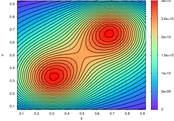
(a) Exact

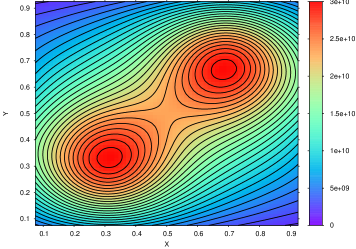
(b) Method-1

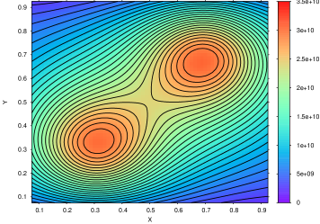
(c) BPM

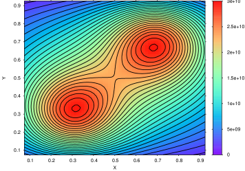
(d) ABC2

Figure 4: The potential $V$ for a superposition of two Gaussian charge densities with centred at $(0.3,0.3,0.3)$ and $(0.7,0.7,0.7)$. A projection on the $XY$ plane $z=0.5$ is shown in each case.

We next consider a unit cube as before with the open faces at $x=0$ and $x=1$m but with a superposition of two Gaussian charge densities:

$$\rho(x,y,z)=\begin{cases}\frac{1}{(\sqrt{2\pi})^{3}\sigma_{x}\sigma_{y}\sigma_{z}}\sum_{i=0}^{1}e^{-\frac{(x-x_{i})^{2}}{2\sigma_{x}^{2}}-\frac{(y-y_{i})^{2}}{2\sigma_{y}^{2}}-\frac{(z-z_{i})^{2}}{2\sigma_{z}^{2}}}\\ ~{}&{}\textstyle\\ 0~{}~{}~{}~{}~{}~{}~{}~{}~{}~{}~{}~{}~{}~{}\mbox{outside the pipe}.\end{cases}$$ (34)

with $\sigma_{x}=\sigma_{y}=\sigma_{z}=1/10$. The results are shown in Fig. (4).

A comparison of the average relative errors can again be found in Table 1. There is a marked improvement in the performance of ABC2 while Method-1 is consistent.

V.1.3 A single Gaussian charge density (Case-3)

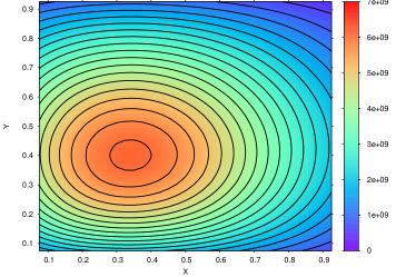
(a) Exact

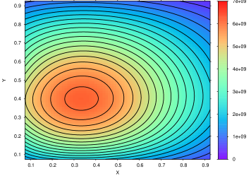
(b) Method-1

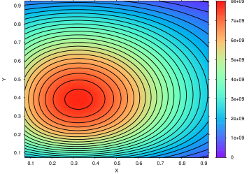
(c) BPM

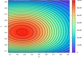
(d) ABC2

Figure 5: The potential $V$ for a single Gaussian charge density centred at $x_{0}=(0.3,0.3,0.3)$. A projection on the $XY$ plane $z=0.5$ is shown in each case.

To understand the reason behind the improvement, we consider a single Gaussian density placed at (0.3,0.3,0.3) but now having $\sigma_{x}=\sigma_{y}=\sigma_{z}=1/3$. The performance of ABC2 is no longer as good and the differences can be seen in Fig. (5). The boundary potential method (BPM) does not perform well either while Method-1 remains consistent and fares reasonably well. Table 1 provides the average relative error in each case. Clearly, Method-1 performs consistently for all density variations when the aspect ratio of the open face is unity while ABC2 performs poorly except in Case-2 where the charge is localized.

To understand this aspect of ABC2, we consider a single Gaussian placed in the centre of the open rectangular pipe and vary the standard deviation $\sigma_{x}$. Since the charge density is now at the centre, the effect on both open faces is now equal. The relative error for ABC2 and Method-1 is shown in Fig. 6. Clearly, the relative error for ABC2 reduces sharply as the charge is localized and saturates for small $\sigma_{x}$ while for Method-1, localization does not change the relative error substantially.

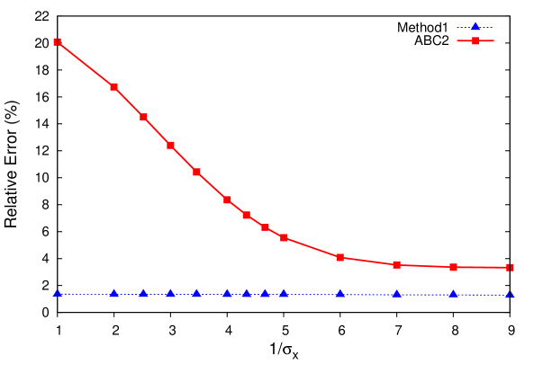
Figure 6: The relative error for $L_{x}=L_{y}=L_{z}=1$ with a Gaussian charge density centred at (0.5,0.5,0.5). The width of the Gaussian varies from $\sigma_{x}=1$ till $\sigma_{x}=1/9$. The error reduces for ABC2 as $\sigma_{x}$ is decreased. For Method-1, the error increases slightly but remains below that of ABC2.

The above observation for ABC2 suggest a relationship between the relative error and the charge density near the open face relative to the peak density in the direction perpendicular to the open face noeffect . When the length $L_{x}$ is fixed, we hypothesize that the error variation with $\sigma_{x}$ (see Fig. 6) depends on how the density varies with $\sigma_{x}$; i.e. Error $\sim\frac{1}{\sigma_{x}}\exp(-A/\sigma_{x}^{2})$ at least for large $\sigma_{x}$. To test this, a $\log$(Error) vs $1/\sigma_{x}^{2}$ plot is shown in Fig. 7 along with the best fitting straight line. For values of $\sigma_{x}$ in the range [1:1/5], the fit is good suggesting that the relative error depends on the density near the open face relative to the peak density in the direction perpendicular to the open face.

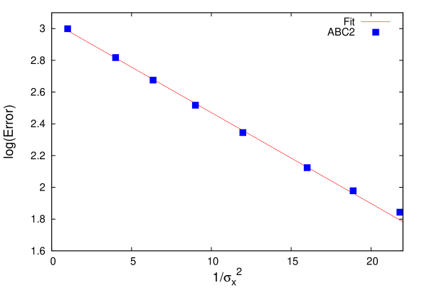
Figure 7: The straight line fit shows that the relative error varies as $\exp(-A/\sigma_{x}^{2})$ for large $\sigma_{x}$

In the above case, while charges were localized on decreasing $\sigma_{x}$, the distance from the open face(s) remained invariant. In order to study the effect of the distance of charge centre from the open face, we nullify the effect of the dominant $\exp(-(x-x_{0})^{2}/2\sigma_{x}^{2})$ term in the Gaussian by scaling the point $x_{0}$ and $\sigma_{x}$ with $L_{x}$. Thus, the relative position of the charge density remains invariant as the length $L_{x}$ is increased. In particular, we choose a single Gaussian charge density with $\sigma_{x}=L_{x}/3$ centred at ($0.3L_{x},0.3L_{y},0.3L_{z}$) and vary $L_{x}$ from 1 to 10. The error decreases for both ABC2 and Method-1 as shown in Fig. 8. This can be ascribed to the increase in the distance of the charge centre from the open faces as $L_{x}$ is increased. A plot of $\log(L_{x})$ vs $\log$(Error) shows (see Fig. 9) that the relative error for large $L_{x}$ decreases inversely as the distance from the charge centre to the open face.

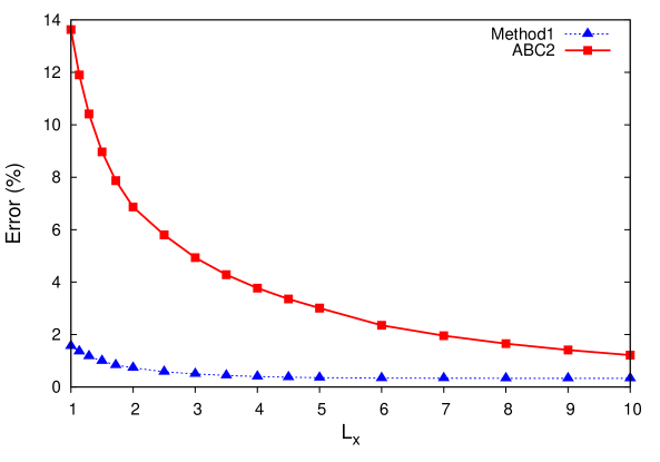
Figure 8: The relative error for $L_{y}=L_{z}=1$ and the length $L_{x}$ varying between 1 and 10 for Method-1 and ABC2. The error for ABC2 reduces with length before saturating.

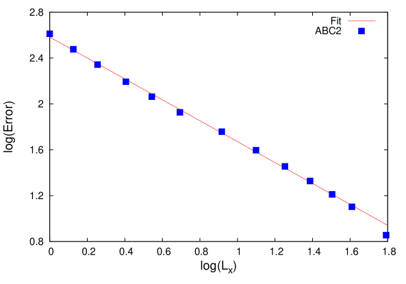
Figure 9: The fitted straight line has a slope -1.07 suggesting that the the relative error varies as $1/L_{x}$ for $L_{x}<4$.

The decrease in relative error with increase in distance of the charge centre from the open face is true for other charge densities as well (including Case-1 where the ABC2 error falls from around 20% at $L_{x}=1$ to 1.6% for $L_{x}=10$). Note that for both small $\sigma_{x}$ and large lengths ($L_{x}$), the error is dominated by other considerations and saturates.

V.2 Large Aspect Ratio

The discussion so far has centred around open faces with unit aspect ratio such as a circular or square aperture. We shall now study the suitability of Method-1 and ABC as the aspect ratio of the open face is altered keeping the length of the pipe unaltered. The discretization can now be done in two ways: (i) the cell aspect ratio can be unity ($h_{x}=h_{y}=h_{z}$) (ii) the cell aspect ratio is the same as that of the computational domain ($h_{x}:h_{y}:h_{z}=L_{x}:L_{y}:L_{z}$). Our studies show that the relative errors are higher when the cell aspect ratio is unity. For the calculations presented below, the cell aspect ratio is same as that of the computational domain.

As the aspect ratio is increased (or decreased) from unity, the domain of convergence of Method-1 decreases and the relative error increases. A comparison of the change in relative error with aspect ratio for ABC-2 and Method-1 is shown in Fig. 10 for a rectangular tube of length $L_{x}=3$ with a single Gaussian charge density placed at ($0.3L_{x},0.3L_{y},0.3L_{z}$) and having $\sigma_{x}=L_{x}/3$, $\sigma_{y}=L_{y}/3$ and $\sigma_{z}=L_{z}/3$. The aspect ratio, $L_{y}/L_{z}$ is varied such that the area of the open face $L_{y}L_{z}=1$. This ensures that the charge density at the open face remains the same as the aspect ratio is varied since $\sigma_{x}\sigma_{y}\sigma_{z}$ is conserved. The relative error using Method-1 in this case rises rapidly for $L_{y}/L_{z}>5$. Thus, Method-1 is suitable in a limited range of aspect ratios.

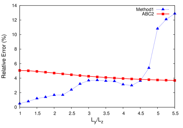
Figure 10: The relative error for aspect ratio $L_{y}/L_{z}>1$ and $L_{x}=3$ for a single Gaussian charge density with $\sigma=L_{x}/3$. The relative error grows rapidly for Method-1 beyond $L_{y}/L_{z}=4$.

The domain of convergence of Method-1 generally shrinks rapidly for aspect ratios beyond $4$. The Asymptotic Boundary Conditions however continue to have a large domain of convergence and can be used for larger aspect ratios. For charges well inside the computational domain and away from the open boundaries, ABC2 performs consistently well irrespective of the aspect ratio. We shall therefore focus on higher order and mixed Asymptotic Boundary Conditions when the relative density of charges is high close to the open boundary.

To this end, we consider six Gaussian charge densities placed such that four of them are at $\sigma_{x}=L_{x}/10$ distance from the open faces while the other two are well inside. With $L_{y}L_{z}=1$, we study the performance of ABC2, ABC3 and a mixture of ABC2 and ABC3 with 5% contribution from ABC2. While, ABC3 is much better than ABC2, the mixture is perhaps the best performer over the range of aspect ratios considered.

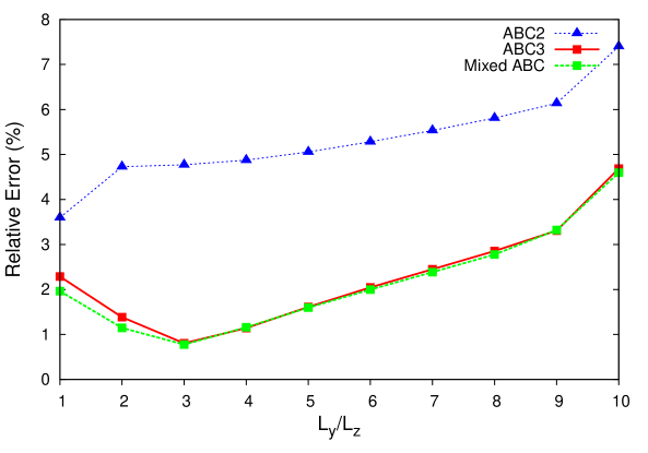
Figure 11: The relative error for $L_{y}/L_{z}\geq 1$ and $L_{x}=3$ for multiple Gaussian charge density with $\sigma=1/10$, four of which are placed near the open faces.

For longer lengths however, the significant advantage of ABC3 decreases and ABC2 performs reasonably well at all aspect ratios considered.

VI Discussion and Summary

We have considered three methods for solving the Poisson equation for open metallic enclosures containing various charge densities. Two of these, the ABCs and BPM, are existing methods that can be directly applied when the computational domain is truncated at the open boundaries. We have, in addition, proposed a non-local truncation (Method-1) based on the solution of the Laplace equation in the charge-free region outside the metallic enclosure.

It is clear from the numerical results that Method-1, as implemented in this paper, is best suited when the aspect ratio of the open face is near unity irrespective of the length of the metallic enclosure. Compared to ABCs, it works especially well when charges are not localized or when the distance from the charge centre to the open face is small. The method uses a 25 term expansion (i.e. truncation of the series at $l_{max}=4$) and for a $81\times 81\times 81$ grid, less than $0.5\%$ of the points on the open boundary need to be matched to determine the unknown expansion coefficients. It is thus non-local but fast and is consistent in performance with errors that may be acceptable in many applications especially when the interior points are of interest. It does however require care in implementation, with the choice of origin and the points used for matching, as major factors especially in asymmetric geometries.

Our studies also reveal that for ABC2, the charge density localization in the direction perpendicular to the open face has a direct bearing on the relative error. The method is best suited when the density falls sharply near the open face from its peak value in the direction perpendicular to the open face. We believe this is due the local nature of the boundary condition. The relative error also depends sensitively on the distance of the charge centre from the open boundary especially when the charge density is not localized. Thus for a density constant in the direction perpendicular to the open face, the error falls as $1/L_{x}$ with the length $L_{x}$.

For larger aspect ratios however, the relative error of Method-1 rises fast and the convergence domain shrinks rapidly. When the aspect ratio of the open face is outside the range [1/4,4], Method-1 is found unsuitable while the local Asymptotic Boundary Conditions (ABC) are stable and give better results. When charges present are closer to the open faces, a combination of 5% ABC2 and 95% ABC3 performs consistently and may be preferred.

References

- (1) V.L.Granatstein and I.Alexeff, High Power Microwave Sources, Artech House, London (1987).
- (2) R.A.Cairns and A.D.R.Phelps, Generation and Application of High Power Microwaves, Institute of Physics Publishing, Bristol (1997).
- (3) J.Berenger, J. Comput. Phys. 114 (1994) 185.
- (4) A.Taflove and S.C.Hagness, Computational Electrodynamics: The Finite-Difference Time-Domain Method, 3rd ed. Artech House Publishers, (2005).
- (5) Q.Chen and A.Konrad, IEEE Trans. Magnetics 33 (1997), 663.
- (6) See for instance A. Cerioni, L. Genovese, A. Mirone1 and V.A. Sole, J. Chem. Phys. 137, 134108 (2012).
- (7) A.Bayliss, M.Gunzberger and E.Turkel, SIAM J. Appl. Math., 42 (1982) 430.
- (8) A.Khebir, A.B.Kouki and R.Mittra, IEEE Trans. Microw. Theory and Techn., 38 (1990) 1427.
- (9) H.Han and X.Wu, Artificial Boundary Method, Tsinghua University Press, Beijing and Springer-Verlag, Heidelberg (2013).
- (10) J.B.Keller and D.Givoli, J. Comput. Phys. 82 (1989) 172.
- (11) I.A.Cermak and P.Silvester, Proc. IEE, 115 (1968) 1341.
- (12) G. H. Miller, J. Comput. Phys. 227 (2008) 7917-7928.
- (13) Z.J.Wang, J. Comput. Phys. 153 (1999) 666-670.
- (14) Z. Ren, F. Bouillault, A. Razek, and J. C. Verite, IEE Proc. Pt. A 135 (1988) 501.
- (15) J.D.Jackson, Classical Electrodynamics, John Wiley and Sons, New York (1999).
- (16) M.V.K.Chari, IEEE Trans. Magnetics 23 (1987) 3566.
- (17) M.V.K.Chari and G.Bedrosian, IEEE Trans. Magnetics 23 (1987) 3572.
- (18) J.Hammel and J.Verboncoeur, 5Th IEEE International Vacuum Electronics Conference, IVEC 2004. 2004:136-137, http://dx.doi.org/10.1109/IVELEC.2004.1316236
- (19) J.Qiang and R.D.Ryne, Comp. Phys. Comm. 138 (2001)18.
- (20) Increasing the peak density while retaining the shape (e.g. by multiplying the Gaussian by a constant) does not have any effect on the relative error.