The thermalization of a two-level atom in a planar dielectric system out of thermal equilibrium

Abstract

We study the thermalization of an elementary quantum system modeled by a two-level atom interacting with stationary electromagnetic fields out of thermal equilibrium near a dielectric slab. The slab is held at a temperature different from that of the region where the atom is located. We find that when the slab is a nonabsorbing and nondispersive dielectric of a finite thickness $d$, no out of thermal equilibrium effects appear as far as the thermalization of the atom is concerned, and a finite thick dielectric slab with a tiny imaginary part in the relative permittivity $\operatorname{Im}\epsilon$ behaves like a half space dielectric substrate if $\frac{\operatorname{Im}\epsilon}{\sqrt{\operatorname{Re}\epsilon-1}}\frac{d}{\lambda_{0}}>1$ is satisfied, where $\lambda_{0}$ is the transition wavelength of the atom. This condition can serve as a guide for an experimental verification, using a dielectric substrate of a finite thickness, of the effects that arise from out of thermal equilibrium fluctuations with a half-space (infinite thickness) dielectric.

I Introduction

Physical systems out of thermal equilibrium but in a stationary configuration, such as that of a substrate and an environment held respectively at different temperatures, may exhibit remarkable and measurable quantum phenomena, and thus have recently attracted an increasing deal of interest both theoretically and experimentally. In this respect, Antezza et al. Antezza investigated, in the large distance limit, the Casimir-Polder (CP) force Casimir in such an out of thermal equilibrium situation. They found that the CP force shows new qualitative and quantitative behaviors. Specifically, the force decays like $1/z^{3}$ and is proportional to $\Delta T^{2}$, where $z$ is the distance between an atom and the surface of the substrate, and $\Delta T^{2}\equiv T_{s}^{2}-T_{e}^{2}$ with $T_{e}$ and $T_{s}$ being respectively the temperatures of the thermal bath in the right and the substrate in the left half space. This behavior of the force differs clearly from that of an atom both in vacuum which has a $1/z^{5}$ dependence Casimir and in a thermal equilibrium environment which behaves like $T/z^{4}$ and is attractive Lifshitz . Actually the out of thermal equilibrium CP force can be either attractive or repulsive depending on the difference of two temperatures. Later, Zhou and Yu analyzed in detail the behaviors of the out of thermal equilibrium CP force of an atom near the surface of a half space real dielectric substrate in different distance regimes Zhou014 , where a real dielectric refers to a nonabsorbing and nondispersive dielectric whose permittivity is real and frequency independent. In addition, the CP force of a diamagnetic atom out of thermal equilibrium has also been investigated in Wu14 . Remarkably, the new behavior of the CP force out of thermal equilibrium has been measured in experiment by positioning a nearly pure ⁸⁷Rb Bose-Einstein condensate a few microns from a dielectric substrate, which consists of uv-grade fused silica with a $2$ mm thickness Obrecht .

On the other hand, the dynamics of an elementary quantum system in a stationary environment out of thermal equilibrium, has been studied by Bellomo et al. Bellomo and it is found that the quantum system modeled by a two-level atom can be thermalized to a steady state with an effective temperature between the temperature of the wall and that of the environment. The similar result has also been obtained for an atom placed outside a radiating Schwarzschild black hole Hu13 . For two quantum emitters interacting with a common stationary electromagnetic field out of thermal equilibrium, Bellomo and Antezza found that the absence of equilibrium allows the generation of steady entangled states between the emitters, which is inaccessible at thermal equilibrium Bellomo13a ; Bellomo13b . In addition, the photon heat tunneling was discussed in Joulain ; Messina12 . Other aspects about the out of thermal equilibrium effects have been discussed in Pitaevskii ; Antezza08 ; Buhmann ; Sherkunov ; Bimonte ; Rodriguez ; Messina ; Kruger ; Kruger11 ; Noto ; Druzhinina ; Behunin ; Leggio ; Zhou15 ; Antezza06 .

To simplify the theoretical calculations, a half-space, even real, dielectric substrate is usually assumed when analyzing the non-equilibrium thermal system. However, in reality, such a dielectric substrate never exists. In fact, in experiment, a dielectric slab with a finite thickness and absorption and dispersion is generally used. As a result, questions naturally arise as to when a generic finite slab can be regarded as an infinite substrate on which the theoretical calculations are based and how the novel out of thermal equilibrium effects depend on the dielectric property. In this paper, we try to answer these questions in terms of the thermalization of a polarizable two-level atom in a thermal bath near a planar dielectric slab out of thermal equilibrium. We will show that for a nonabsorbing and nondispersive dielectric with a finite thickness NO out of thermal equilibrium effects appear as far as the thermalization of the atom is concerned. So, to have non vanishing out of thermal equilibrium effects, one has to have a real dielectric substrate with an infinite thickness or a complex dielectric substrate. Since the infinitely thick substrate does not really exist, we give the condition when a dielectric with a tiny nonzero imaginary part in the relative permittivity with a finite thickness can be regarded as a half-space dielectric. This puts on the solid foundation the experimental test using a finite dielectric substrate of theoretical predictions for novel effects from out of thermal equilibrium based upon a half-space dielectric.

II Open quantum system

We examine in the framework of open quantum systems the thermalization of a two-level atom near a dielectric substrate in a stationary configuration out of thermal equilibrium. We assume that two stationary states of the atom are represented by $|1\rangle$ and $|2\rangle$ respectively, and the energy spacing is $\hbar\omega_{0}$. A planar dielectric slab with thickness $d$ is placed in a thermal bath at temperature $T_{0}$ and its right surface coincides with the $z=0$ plane. The slab is assumed to be in local thermal equilibrium at a different temperature $T_{1}$ (See Fig. 1). The atom is at the position $z_{A}>0$ in the empty space. So, the whole system is out of thermal equilibrium but in a stationary regime and the total Hamiltonian that governs the evolution of the system takes the form

$${H}={H}_{A}+{H}_{B}+{H}_{I}\;,$$ (1)

where ${H}_{A}=\sum_{m=1}^{2}\omega_{m}|m\rangle\langle m|$ is the Hamiltonian of the atom, ${H}_{B}$ is the Hamiltonian describing the environment the atom is coupled to, and ${H}_{I}$ denotes the interaction between the atom and the environment, which takes the form ${H}_{I}=-{\bm{D}(t)}\cdot{\bm{E}}(\bm{r},t)$ in the multipolar coupling scheme. Here, ${\bm{D}(t)}$ is the electric dipole moment of the atom, and ${\bm{E}}(\bm{r},t)$ is the electric field strength.

In the interaction picture, the total density matrix $\rho_{tot}(t)$ of the system satisfies the von Neumann equation

$$\frac{\mathrm{d}}{\mathrm{d}t}\rho_{\text{tot}}(t)=-\frac{\mathrm{i}}{\hbar}[H_{I},\rho_{\text{tot}}(t)]\;,$$ (2)

with the initial state being described by $\rho_{tot}(0)=\rho(0)\otimes\rho_{B}$, where $\rho(0)$ is the initial density matrix of the atom and $\rho_{B}$ is that of the environment. $H_{I}$ can be rewritten as

$$H_{I}=-\sum_{i,\omega}e^{-\mathrm{i}\omega t}A_{i}(\omega)E_{i}(\mathbf{r},t)\;,$$ (3)

where $i\in\{x,y,z\}$ and $A_{i}(\omega)=\sum_{\varepsilon^{\prime}-\varepsilon=\omega}\Pi(\varepsilon)D_{i}\Pi(\varepsilon^{\prime})$. $\Pi(\varepsilon)$ denotes the projection onto the eigenspace belonging to the eigenvalue $\varepsilon$ of $H_{A}$, which means that $A_{i}(\omega)$ are the eigenoperators of $H_{A}$. Tracing $\rho_{\text{tot}}(t)$ over the degrees of freedom associated with the environment, one can obtain the reduced density matrix $\rho(t)$ for the atom, namely, $\rho(t)=\operatorname{Tr}_{B}\,[\rho_{\text{tot}}(t)]$, which, in the limit of weak coupling, obeys the master equation

$$\frac{\mathrm{d}}{\mathrm{d}t}\rho(t)=-\frac{\mathrm{i}}{\hbar}[H_{LS},\rho(t)]+\mathcal{D}(\rho(t))\;,$$ (4)

where

$$H_{LS}=\hbar\sum_{\omega}\sum_{i,j}s_{ij}(\omega)A_{i}^{\dagger}(\omega)A_{j}(\omega)$$ (5)

is the so-called Lamb-shift Hamiltonian since it produces shifts of the atomic energy levels, and

$$\mathcal{D}(\rho(t))=\sum_{\omega}\sum_{i,j}\gamma_{ij}(\omega)[A_{j}(\omega)\rho(t)A_{i}^{\dagger}(\omega)-\frac{1}{2}\{A_{i}^{\dagger}(\omega)A_{j}(\omega),\rho(t)\}]$$ (6)

is the dissipator. Here,

$$\gamma_{ij}(\omega)=\frac{1}{\hbar^{2}}\int_{-\infty}^{\infty}\mathrm{d}se^{\mathrm{i}\omega s}\langle E_{i}(\bm{r},s)E_{j}(\bm{r},0)\rangle$$ (7)

is the Fourier transforms to the reservoir correlation function $\langle E_{i}(\bm{r},s)E_{j}(\bm{r},0)\rangle$, while $s_{ij}$ is related to $\gamma_{ij}$ through

$$s_{ij}(\omega)=\frac{\mathrm{i}}{2}\gamma_{ij}-\mathrm{i}\tau_{ij}(\omega)\;,$$ (8)

where $\tau_{ij}(\omega)=\frac{1}{\hbar^{2}}\int_{0}^{\infty}\mathrm{d}se^{\mathrm{i}\omega s}\langle E_{i}(\bm{r},s)E_{j}(\bm{r},0)\rangle$ is the one-side Fourier transforms. With the help of $\frac{1}{x\mp\mathrm{i}\epsilon}=\mathrm{P}\frac{1}{x}\pm\mathrm{i}\pi\delta(x)$, where $\mathrm{P}$ denotes the Cauchy principal value, $s_{ij}(\omega)$ can be re-expressed as

$$s_{ij}(\omega)=-\frac{\mathrm{P}}{2\pi}\int_{-\infty}^{\infty}\frac{\gamma_{ij}(z)}{z-\omega}\mathrm{d}z\;.$$ (9)

For a two-level atom, the atomic dipole operator can be written as

$$\bm{D}(t)=\bm{d}_{21}|2\rangle\langle 1|e^{-\mathrm{i}\omega_{0}t}+\bm{d}^{*}_{21}|1\rangle\langle 2|e^{\mathrm{i}\omega_{0}t}\;,$$ (10)

which implies that $\bm{A}(\omega)=\sum_{\omega}\bm{d}_{21}|2\rangle\langle 1|=\bm{A}^{\dagger}(-\omega)$. Since the summation over $\omega$ just contains two terms: $\omega=\omega_{0}$ and $\omega=-\omega_{0}$, the master equation becomes

$$\frac{\mathrm{d}}{\mathrm{d}t}\rho(t) = -\mathrm{i}\bigg{[}\sum_{n=1}^{2}\omega_{n}|n\rangle\langle n|+S(\omega_{0})|2\rangle\langle 2|+S(-\omega_{0})|1\rangle\langle 1|,\rho(t)\bigg{]}$$

$$+ \Gamma(\omega_{0})\bigg{(}\rho_{22}|1\rangle\langle 1|-\frac{1}{2}\{|2\rangle\langle 2|,\rho(t)\}\bigg{)}+\Gamma(-\omega_{0})\bigg{(}\rho_{11}|2\rangle\langle 2|-\frac{1}{2}\{|1\rangle\langle 1|,\rho(t)\}\bigg{)}\;,$$

where

$$S(\omega_{0}) \equiv \sum_{i,j}s_{ij}(\omega_{0})[\bm{d}_{21}]_{i}^{*}[\bm{d}_{21}]_{j}\;,$$ (12)

$$S(-\omega_{0}) \equiv \sum_{i,j}s_{ij}(-\omega_{0})[\bm{d}_{21}]_{i}[\bm{d}_{21}]_{j}^{*}\;,$$

$$\Gamma(\omega_{0}) \equiv \sum_{i,j}\gamma_{ij}(\omega_{0})[\bm{d}_{21}]_{i}^{*}[\bm{d}_{21}]_{j}\;,$$ (13)

$$\Gamma(-\omega_{0}) \equiv \sum_{i,j}\gamma_{ij}(-\omega_{0})[\bm{d}_{21}]_{i}[\bm{d}_{21}]_{j}^{*}\;.$$

Here, $S(-\omega_{0})$ and $S(\omega_{0})$ represent the atomic eigenvalue shifts of the ground state and the excited one, respectively, and the corresponding energy shifts are $\delta E_{1}=\hbar S(-\omega_{0})$ and $\delta E_{2}=\hbar S(\omega_{0})$. As a result, the Lamb shift (the relative energy shift) is given by $\Delta=\delta E_{2}-\delta E_{1}$. $\Gamma(-\omega_{0})$ and $\Gamma(\omega_{0})$ are the downward and upward transition rates respectively, which are related with the thermalization of an atom. Therefore, in the following only $\gamma_{ij}(\omega)$ is analyzed. From its definition, we have

$$\gamma_{ij}(\omega) = \frac{1}{\hbar^{2}}\int_{-\infty}^{\infty}\mathrm{d}s\int_{0}^{\infty}\mathrm{d}\omega^{\prime}\int_{0}^{\infty}\mathrm{d}\omega^{\prime\prime}[e^{\mathrm{i}(\omega-\omega^{\prime\prime})s}\langle E_{i}(\bm{r},\omega^{\prime\prime})E_{j}^{\dagger}(\bm{r},\omega^{\prime})\rangle$$

$$+e^{\mathrm{i}(\omega+\omega^{\prime\prime})s}\langle E_{i}^{\dagger}(\bm{r},\omega^{\prime\prime})E_{j}(\bm{r},\omega^{\prime})\rangle]$$

$$= \frac{2\pi}{\hbar^{2}}\int_{0}^{\infty}\mathrm{d}\omega^{\prime}\begin{cases}\langle E_{i}(\bm{r},\omega)E_{j}^{\dagger}(\bm{r},\omega^{\prime})\rangle&\omega>0\\ \langle E_{i}^{\dagger}(\bm{r},-\omega)E_{j}(\bm{r},\omega^{\prime})\rangle&\omega<0\end{cases}\;,$$

where $\langle E_{i}(\bm{r},\omega)E_{j}(\bm{r},\omega^{\prime})\rangle=\langle E_{i}^{\dagger}(\bm{r},\omega)E_{j}^{\dagger}(\bm{r},\omega^{\prime})\rangle=0$ and $\int_{-\infty}^{\infty}\mathrm{d}s\exp(-\mathrm{i}\epsilon s)=2\pi\delta(\epsilon)$ have been used.

For a nonmagnetic medium, the electric field operator can be expressed as

$${\bm{E}}(\bm{r},\omega) \!= \!\mathrm{i}\,\frac{\omega^{2}}{c^{2}}\sqrt{\frac{\hbar}{\pi\epsilon_{0}}}\int\mathrm{d}^{3}r^{\prime}\,\sqrt{\operatorname{Im}\epsilon(\bm{r}^{\prime},\omega)}\,\mbox{{{{G}}}}(\bm{r},\bm{r}^{\prime},\omega)\!\cdot\!{\bm{f}}(\bm{r}^{\prime},\omega)\;.$$ (15)

Here, $\epsilon_{0}$ and $\epsilon$ are the vacuum and relative permittivity, respectively, G is the classical Green’s tensor, which satisfies an useful integral relation

$$\int\mathrm{d}^{3}s\,\operatorname{Im}\epsilon(\bm{s},\omega)\,\mbox{{{{G}}}}(\bm{r},\bm{s},\omega)\!\cdot\!\mbox{{{{G}}}}^{\ast\mathsf{T}}(\bm{r}^{\prime},\bm{s},\omega)=\frac{c^{2}}{\omega^{2}}\operatorname{Im}\mbox{{{{G}}}}(\bm{r},\bm{r}^{\prime},\omega)\;,$$ (16)

and ${\bm{f}}(\bm{r},\omega)$ and ${\bm{f}}^{\dagger}(\bm{r},\omega)$ are the annihilation and creation operators of the elementary electric excitations, respectively. They obey the bosonic commutation relations $[{\bm{f}}(\bm{r},\omega),{\bm{f}}^{\dagger}(\bm{r}^{\prime},\omega^{\prime})]=\bm{\delta}(\bm{r}-\bm{r}^{\prime})\delta(\omega-\omega^{\prime})$ and $[{\bm{f}}(\bm{r},\omega),{\bm{f}}(\bm{r}^{\prime},\omega^{\prime})]=[{\bm{f}}^{\dagger}(\bm{r},\omega),{\bm{f}}^{\dagger}(\bm{r}^{\prime},\omega^{\prime})]=\mbox{{{{0}}}},$ where 0 represents a zero matrix. For the thermal state describing the system in a stationary configuration out of thermal equilibrium we are considering, one has

$$\langle\{\beta_{i}\}|{\bm{f}}(\bm{r},\omega){\bm{f}}^{\dagger}(\bm{r}^{\prime},\omega^{\prime})|\{\beta_{i}\}\rangle=[1+N(\omega,\beta_{i})]\delta(\bm{r}-\bm{r}^{\prime})\delta(\omega-\omega^{\prime})\;,$$ (17)

$$\langle\{\beta_{i}\}|{\bm{f}}^{\dagger}(\bm{r},\omega){\bm{f}}(\bm{r}^{\prime},\omega^{\prime})|\{\beta_{i}\}\rangle=N(\omega,\beta_{i})\delta(\bm{r}-\bm{r}^{\prime})\delta(\omega-\omega^{\prime})\;,$$ (18)

where $\beta_{i}=\hbar c/kT_{i}$ with $i=0$ or $1$, and $N(\omega,\beta_{i})=\frac{1}{e^{\beta_{i}\omega/c}-1}$. Substituting Eq. (15) into Eq. (II) and considering the relations given in Eqs. (17, 18), we have

$$\gamma_{ij}(\omega)=\frac{2\mu_{0}\omega^{4}}{\hbar c^{2}}\int\mathrm{d}^{3}{r}^{\prime}[1+N(\omega,\beta)]\operatorname{Im}\epsilon(\bm{r}^{\prime},\omega){G}_{ik}(\bm{r},\bm{r}^{\prime},\omega){G}^{*}_{jk}(\bm{r},\bm{r}^{\prime},\omega)\;,$$ (19)

and

$$\gamma_{ij}(-\omega)=\frac{2\mu_{0}\omega^{4}}{\hbar c^{2}}\int\mathrm{d}^{3}{r}^{\prime}\,N(\omega,\beta)\operatorname{Im}\epsilon(\bm{r}^{\prime},\omega){G}_{ik}(\bm{r},\bm{r}^{\prime},\omega){G}^{*}_{jk}(\bm{r},\bm{r}^{\prime},\omega)\;.$$ (20)

Here $\mu_{0}$ is the vacuum permeability and $\mu_{0}\epsilon_{0}=1/c^{2}$ is used.

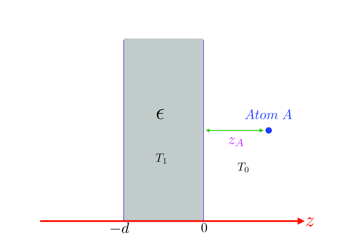
Figure 1: (color online). Scheme of the system considered.

For an atom near a dielectric slab described in Fig. 1, Eqs. (19, 20) become

$$\gamma_{ij}(\omega) = \frac{2\mu_{0}\omega^{2}}{\hbar}[1+N(\omega,\beta_{0})]\operatorname{Im}G_{ij}(\bm{r}_{A},\bm{r}_{A},\omega)$$

$$+\frac{2\pi}{\hbar}[N(\omega,\beta_{1})-N(\omega,\beta_{0})]\,g_{ij}(\bm{r}_{A},\bm{r}_{A},\omega)\;,$$

and

$$\gamma_{ij}(-\omega) = \frac{2\mu_{0}\omega^{2}}{\hbar}N(\omega,\beta_{0})\operatorname{Im}G_{ij}(\bm{r}_{A},\bm{r}_{A},\omega)$$

$$+\frac{2\pi}{\hbar}\,[N(\omega,\beta_{1})-N(\omega,\beta_{0})]\,g_{ij}(\bm{r}_{A},\bm{r}_{A},\omega)\;,$$

where Eq. (16) has been used, and

$$g_{ij}(\bm{r},\bm{r},\omega)\equiv\frac{\mu_{0}\omega^{4}}{\pi c^{2}}\int\mathrm{d}^{2}\bm{r}^{\prime}_{\|}\int^{0}_{-d}\mathrm{d}z^{\prime}\operatorname{Im}\epsilon\,{G}_{ik}(\bm{r},\bm{r}^{\prime},\omega){G}^{*}_{jk}(\bm{r},\bm{r}^{\prime},\omega)\;,$$ (23)

with $\bm{r}^{\prime}_{\|}=\{x^{\prime},y^{\prime}\}$. In the right hand side of Eqs. (II, II), the first term gives the contributions of the zero-point fluctuations and the thermal fluctuations in thermal equilibrium at a temperature $T_{0}$, while the second term arises from the out of thermal equilibrium nature of the system. For the system we are considering, only the diagonal elements of $\operatorname{Im}G_{ij}(\bm{r},\bm{r},\omega)$ and $g_{ij}(\bm{r},\bm{r},\omega)$ are non-vanishing.

III Thermalization

Using Eqs. (II, II), we can show that the transition rates $\Gamma(\omega_{0})$ and $\Gamma(-\omega_{0})$ can be re-expressed as

$$\begin{split}\begin{pmatrix}\Gamma(\omega_{0})\\ \Gamma(-\omega_{0})\end{pmatrix}&=\alpha(\omega_{0})\Gamma_{0}(\omega_{0})\begin{pmatrix}1+N_{\text{eff}}(\omega_{0})\\ N_{\text{eff}}(\omega_{0})\end{pmatrix},\end{split}$$ (24)

where $\Gamma_{0}(\omega_{0})=\frac{\omega_{0}^{3}|\mathbf{d}_{12}|^{2}}{3\pi\epsilon_{0}\hbar c^{3}}$ is the vacuum spontaneous-emission rate related to the transition between the ground and exited states,

$$\alpha(\omega_{0})=\frac{6\pi c}{\omega_{0}}\sum_{i,j}\frac{[\bm{d}_{21}]_{i}[\bm{d}_{21}]_{j}^{*}}{|\bm{d}_{21}|^{2}}\text{Im}G_{ij}(\bm{r},\bm{r},\omega_{0})\;,$$ (25)

and

$$N_{\text{eff}}(\omega_{0}) = N(\omega_{0},\beta_{0})+\frac{6\pi^{2}c}{\mu_{0}\omega_{0}^{3}\alpha(\omega_{0})}[N(\omega_{0},\beta_{1})-N(\omega_{0},\beta_{0})]\sum_{i,j}\frac{[\bm{d}_{21}]_{i}[\bm{d}_{21}]_{j}^{*}}{|\bm{d}_{21}|^{2}}g_{ij}(\bm{r}_{A},\bm{r}_{A},\omega_{0})$$ (26)

$$= N(\omega_{0},\beta_{0})+\frac{2\pi^{2}c}{\mu_{0}\omega_{0}^{3}\alpha(\omega_{0})}\,[N(\omega_{0},\beta_{1})-N(\omega_{0},\beta_{0})]\operatorname{g}(\bm{r}_{A},\bm{r}_{A},\omega_{0})\;.$$

Here, the last line holds for an isotropically polarizable atom, and $g=g_{xx}+g_{yy}+g_{zz}$. So, $N_{\text{eff}}(\omega_{0})$ depends on the temperature $T_{i}$ ($i=0,1$) and the dielectric property of slab encoded in function $g(\bm{r},\bm{r},\omega)$. As discussed in Bellomo ; Hu13 , after evolving for a sufficiently long period of time, the atom will be thermalized to a steady state with an effective temperature

$$T_{\text{eff}}=\frac{\hbar\omega_{0}}{k}[\ln(1+N_{\text{eff}}^{-1}(\omega_{0}))]^{-1}\;.$$ (27)

It is easy to see that if the substrate is in thermal equilibrium with the thermal radiation in the empty space where the atom is located, then $T_{\text{eff}}$ reduces to $T_{0}$ as expected.

In order to analyze in detail the thermalization temperature of the atom, we first need to examine the behavior of $\operatorname{g}(\bm{r},\bm{r},\omega)$, which depends on the Green’s function $\mbox{{{{G}}}}(\omega,\bm{r},\bm{r^{\prime}})$, where $\bm{r}$ indicates the position of the atom and thus it is restricted to the empty right half-space, while $\bm{r}^{\prime}$ is in the slab. For the system considered, the Green’s function can be expanded as

$$\mbox{{{{G}}}}(\omega,\bm{r},\bm{r}^{\prime})=\int d^{2}\bm{k}\;e^{\mathrm{i}\bm{k}\cdot(\bm{r}_{\|}-\bm{r}^{\prime}_{\|})}\mbox{{{{G}}}}(\bm{k},\omega,z,z^{\prime})$$ (28)

where $\bm{k}=(k_{x},k_{y})$. Since $z$ and $z^{\prime}$ are in different regions, from Refs. Tomas1995 ; Chew we have that

$$\mbox{{{{G}}}}(\bm{k},\omega,z,z^{\prime}) = \frac{\mathrm{i}}{8\pi^{2}b_{0}(k)}\sum_{\sigma=s,p}\xi^{\sigma}\frac{t^{\sigma}(k)e^{\mathrm{i}b_{0}(k)z}}{D^{\sigma}(k)}\cdot$$ (29)

$$\hat{\bm{e}}_{\sigma_{0}}^{+}(\bm{k})\big{[}\hat{\bm{e}}_{\sigma_{1}}^{-}(-\bm{k})e^{-\mathrm{i}b_{1}(k)z^{\prime}}+r^{\sigma}_{-}(k)\hat{\bm{e}}_{\sigma_{1}}^{+}(-\bm{k})e^{\mathrm{i}b_{1}(k)(z^{\prime}+2d)}\big{]}\;,$$

where $\xi^{p}=1$, $\xi^{s}=-1$, $b_{0}(k)=\sqrt{k_{0}^{2}-k^{2}}$, $b_{1}(k)=\sqrt{k_{1}^{2}-k^{2}}$, $k=|\bm{k}|$, $k_{0}=\frac{\omega}{c}$, $k_{1}=\sqrt{\epsilon}\frac{\omega}{c}$, and

$$D^{\sigma}(k)=1-r^{\sigma}_{-}r^{\sigma}_{+}(k)e^{2\mathrm{i}b_{1}(k)d}\,,$$

with $r^{\sigma}_{+}(k)$ and $r^{\sigma}_{-}(k)$ being the reflection coefficients at the right and left boundaries of the slab, which have the forms:

$$r^{s}_{\pm}(k)=\frac{b_{1}(k)-b_{0}(k)}{b_{1}(k)+b_{0}(k)}\;,\quad r^{p}_{\pm}(k)=\frac{b_{1}(k)-\epsilon b_{0}(k)}{b_{1}(k)+\epsilon b_{0}(k)}\;.$$ (30)

$t^{\sigma}(k)=\sqrt{\frac{1}{\epsilon}}(1-r^{\sigma}_{+}(k))$ is the transmission coefficient between the empty space and the slab. In addition, we define

$$\hat{\bm{e}}_{p_{i}}^{\pm}(\bm{k})={\frac{1}{k_{i}}}(\mp b_{i}\hat{\bm{k}}+k\hat{\bm{z}})\;,\quad\hat{\bm{e}}_{s_{i}}^{\pm}(\bm{k})=\hat{\bm{k}}\times\hat{\bm{z}}\;.$$ (31)

Substituting Eqs. (28, 29) into Eq. (23), for a system described in Fig. 1 and an isotropically polarizable atom, one has $\operatorname{g}(\bm{r},\bm{r},\omega)=g(z,z,\omega)$ with

$$g(z,z,\omega) = \frac{\mu_{0}\omega^{2}}{8\pi^{2}}\int_{0}^{\infty}\frac{k\mathrm{d}k}{|b_{0}(k)|^{2}}e^{-2\operatorname{Im}b_{0}(k)z}\bigg{\{}\operatorname{Re}b_{1}(k)[A_{+}(k)+{A}(k)](1-e^{-2\operatorname{Im}b_{1}(k)d})$$

$$+e^{-2\operatorname{Im}b_{1}(k)d}\bigg{(}\operatorname{Re}b_{1}(k)[A_{+}(k)|r^{p}_{-}(k)|^{2}+{A}(k)|r^{s}_{-}(k)|^{2}](1-e^{-2\operatorname{Im}b_{1}(k)d})$$

$$+2\operatorname{Im}b_{1}(k)[A_{-}(k)\operatorname{Re}r^{p}_{-}(k)+{A}(k)\operatorname{Re}r^{s}_{-}(k)]\sin(2\operatorname{Re}b_{1}(k)d)$$

$$+2\operatorname{Im}b_{1}(k)[A_{-}(k)\operatorname{Im}r^{p}_{-}(k)+{A}(k)\operatorname{Im}r^{s}_{-}(k)][\cos(2\operatorname{Re}b_{1}(k)d)-1]\bigg{)}\bigg{\}}\;.$$

where

$$A_{\pm}(k)=|\frac{t^{p}(k)}{D^{p}(k)}|^{2}\frac{[k^{2}\pm|b_{1}(k)|^{2}][k^{2}+|b_{0}(k)|^{2}]}{|k_{0}k_{1}|^{2}}\;,\quad{A}(k)=|\frac{t^{s}(k)}{D^{s}(k)}|^{2}\;.$$ (33)

This expression shows that $\operatorname{Im}b_{0}(k)$ must be nonzero, otherwise $g(z,z,\omega)$ will become a constant independent of $z$. From the definition of $b_{0}({k})$ and $b_{1}({k})$, we obtain that

$$2\operatorname{Im}^{2}b_{0}(k)=-\big{(}\frac{\omega^{2}}{c^{2}}-k^{2}\big{)}+|\frac{\omega^{2}}{c^{2}}-k^{2}|$$ (34)

and

$$\operatorname{Im}^{2}b_{1}(k) = \frac{1}{2}\bigg{[}-\bigg{(}\frac{\omega^{2}}{c^{2}}\operatorname{Re}\epsilon-k^{2}\bigg{)}+\sqrt{\frac{\omega^{4}}{c^{4}}\operatorname{Im}^{2}\epsilon+\bigg{(}\frac{\omega^{2}}{c^{2}}\operatorname{Re}\epsilon-k^{2}\bigg{)}^{2}}\,\bigg{]}\;,$$ (35)

$$\operatorname{Re}^{2}b_{1}(k) = \frac{1}{2}\bigg{[}\bigg{(}\frac{\omega^{2}}{c^{2}}\operatorname{Re}\epsilon-k^{2}\bigg{)}+\sqrt{\frac{\omega^{4}}{c^{4}}\operatorname{Im}^{2}\epsilon+\bigg{(}\frac{\omega^{2}}{c^{2}}\operatorname{Re}\epsilon-k^{2}\bigg{)}^{2}}\,\bigg{]}\;.$$ (36)

A nonzero $\operatorname{Im}b_{0}(k)$ means that $k^{2}>\frac{\omega^{2}}{c^{2}}$ and thus only the $k>\frac{\omega}{c}$ interval in $k$ integration from $0$ to $\infty$ contributes. Let us note that $\operatorname{Im}^{2}b_{1}(k)$ is an increasing function of $k^{2}$, while $\operatorname{Re}^{2}b_{1}(k)$ is a decreasing one, as is shown graphically in Fig. 2.

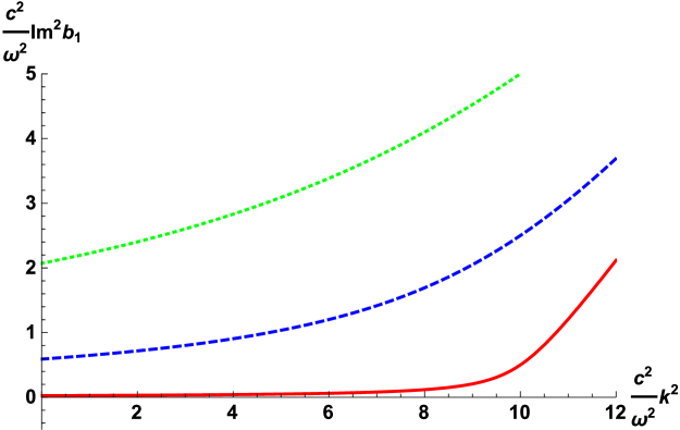
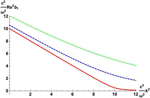
Figure 2: (color online). The evolutionary curves of $\frac{c^{2}}{w^{2}}\operatorname{Im}^{2}b_{1}$ (left panel) and $\frac{c^{2}}{w^{2}}\operatorname{Re}^{2}b_{1}$ (right panel) with respect to $\frac{c^{2}}{w^{2}}k^{2}$ with $\operatorname{Re}\epsilon=10$. The red solid, blue dashed and green dotted lines correspond to $\operatorname{Im}\epsilon=1$, $5$ and $10$, respectively.

If the slab consists of real dielectrics, i.e., $\operatorname{Im}\epsilon=0$, Eqs. (35, 36) tell us that $\operatorname{Im}b_{1}(k)=0$, if $\operatorname{Re}b_{1}(k)\neq 0$, and vice versa. As a result, it is easy to see that $g(z,z,\omega)=0$. Only when the slab thickness is infinite, that is, $d\rightarrow\infty$ and $r^{\sigma}_{-}=0$, is $g(z,z,\omega)$ nonzero and it then becomes

$$g(z,z,\omega) = \frac{\mu_{0}\omega^{2}}{8\pi^{2}}\int_{0}^{\infty}\frac{k\mathrm{d}k}{|b_{0}(k)|^{2}}e^{-2\operatorname{Im}b_{0}(k)z}\operatorname{Re}b_{1}(k)[\bar{A}_{+}(k)+\bar{A}(k)]$$ (37)

where

$$\bar{A}_{+}(k)=|t^{p}(k)|^{2}\frac{[k^{2}+|b_{1}(k)|^{2}][k^{2}+|b_{0}(k)|^{2}]}{|k_{0}k_{1}|^{2}}\;,\quad\bar{A}(k)=|t^{s}(k)|^{2}\;.$$ (38)

This demonstrates that there is NO out of thermal equilibrium effect for any real dielectric substrate of finite thickness even when the substrate is held at a different local temperature. In other words, an infinite thickness is the only way to have an out thermal equilibrium effect for a real dielectric substrate.

Another way to have a nonzero out of thermal equilibrium effect is that the slab consists of the dispersive and absorbing dielectric ($\operatorname{Im}\epsilon\neq 0$). This is similar to what happens to the decay rate of the exited state of an atom in front of a dielectric plate, which is proportional to the imaginary part of the permittivity and also equals to zero when $\operatorname{Im}\epsilon=0$ DF . From the Eq. (III), one can see that, if $2\operatorname{Im}b_{1}(k)d>1$, the terms depending on $d$ can be neglected since they are exponentially suppressed as compared to the other term, which then gives the dominant contribution. In this case, the result of the integral becomes effectively independent of $d$ and approximates to that in the case of a half-space dielectric substrate, which has the same form as that given in Eq. (37). Since $\operatorname{Im}^{2}b_{1}(k)$ is an increasing function of $k^{2}$ and $k^{2}>\frac{\omega^{2}}{c^{2}}$ is required, the minimum value of $\operatorname{Im}b_{1}(k)$ is achieved at $k^{2}=\frac{\omega^{2}}{c^{2}}$

$${\text{Min}}\{\operatorname{Im}b_{1}(k)\}=\frac{1}{\sqrt{2}}\frac{\omega}{c}\bigg{[}-(\operatorname{Re}\epsilon-1)+\sqrt{\operatorname{Im}^{2}\epsilon+(\operatorname{Re}\epsilon-1)^{2}}\bigg{]}^{1/2}\;.$$ (39)

So, the condition for the thermalization of an two-level atom with a typical transition $\omega_{0}$ near a dielectric slab of finite thickness $d$ out of thermal equilibrium to behave like that near an infinitely thick half-space dielectric substrate is

$$\frac{\sqrt{2}d}{\lambda_{0}}\bigg{[}-(\operatorname{Re}\epsilon-1)+\sqrt{\operatorname{Im}^{2}\epsilon+(\operatorname{Re}\epsilon-1)^{2}}\bigg{]}^{1/2}>1\;,$$ (40)

where $\lambda_{0}=\frac{c}{\omega_{0}}$ is the transition wavelength of the atom. Since the dielectrics with a very small but nonzero $\operatorname{Im}\epsilon$, such as fused silica and sapphire, are used in the experiment to observe the novel feature for the CP force out of thermal equilibrium Obrecht , we expand the condition in the limit of $\operatorname{Im}\epsilon\sim 0$ and obtain

$$\frac{\operatorname{Im}\epsilon}{\sqrt{\operatorname{Re}\epsilon-1}}\frac{d}{\lambda_{0}}>1\;.$$ (41)

Obviously, for a given atom we can always find a finite $d$ so that the condition is satisfied as long as $\operatorname{Im}\epsilon$ is not vanishing no matter how small it is. Since mathematically infinite thick slab does not exist, the above relation can serve as a guide for an experimental verification of the effects that arise from out of thermal equilibrium fluctuations, and makes it justified to test experimentally the novel property theoretically found from a half-space dielectric out of thermal equilibrium using a dielectric substrate of finite thickness with a tiny imaginary part in the relative permittivity.

Now a few comments are in order. First, our results can be generalized to a system of a multilayer dielectric body with each layer of a different permittivity in local thermal equilibrium at a different temperature. For the multilayered substrate consisting of only real dielectric, if the outermost left layer is a perfect mirror or empty space, the system has no out of thermal equilibrium effect at least as far as the thermalization of the atom is concerned. If the outermost left layer is a half-space substrate at a certain temperature, only this temperature and that of the thermal bath in the right half empty space affect the thermalization of the atom. Second, although, our calculations are performed under the assumption of an isotropically polarizable atom, our conclusions also hold for an anisotropically polarizable atom since the only difference for such a case is that the definitions of ${A}_{\pm}(k)$ and ${A}(k)$ in Eq. (III) are different. Finally, here we only investigate the thermalization of an atom in front of a slab. The out of thermal equilibrium Casimir-Polder force, especially its explicit dependence on the thickness $d$, the distance $z_{A}$ and the temperatures $T_{i}$ in different limits like what was discussed in DF for the thermal Casimir-Polder force is an interesting topic which is currently under investigation.

IV Conclusion

In conclusion, we have studied the thermalization of a two-level atom near a planar dielectric substrate in a stationary environment out of thermal equilibrium in which the atom is located in an empty space filled with a thermal bath at a temperature different from the local thermal equilibrium temperature of the substrate. We demonstrate that when the planar dielectric substrate is a real dielectric of finite thickness, no out of thermal equilibrium effects appear as far as the thermalization of the atom is concerned. That is to say, the atom thermalizes as if the substrate is in thermal equilibrium with the thermal bath in the empty space where the atom is located. We also show that a planar dispersive and absorbing dielectric substrate with a finite thickness and a tiny imaginary part in the relative permittivity, in its influence on the thermalization of the atom, behaves like a half-space dielectric under certain condition, and we concretely derive this condition in our paper, which can serve as a guide for an experimental verification, using a dielectric substrate of a finite thickness, of the effects that arise from out of thermal equilibrium fluctuations with a half-space (infinite thickness) dielectric.

References

(1)M. Antezza, L. P. Pitaevskii, and S. Stringari, Phys. Rev. Lett.
95, 113202 (2005); M. Antezza, J. Phys. A 39, 6117 (2006).
(2) H. B. G. Casimir and D. Polder, Phys. Rev. 73, 360 (1948).