Outage Bound for Max-Based Downlink Scheduling With Imperfect CSIT and Delay Constraint

Abstract

We consider downlink max-based scheduling in which the base station and each user are equipped with a single antenna. In each time slot, the base station obtains channel gains of all users and selects the user with the largest squared channel gain. Assuming that channel state information at the transmitter (CSIT), i.e., squared channel gain, can be inaccurate, we derive lower bounds for probability of outage, which occurs when a required data rate is not satisfied under a delay constraint. The bounds are tight for Rayleigh fading and show how required rate and CSIT error affect outage performance.

I Introduction

Imperfect channel state information at the transmitter (CSIT) can adversely affect the performance of wireless communication systems [1, see the references therein]. In [2], a base station is assumed to only have a noisy estimate of user’s signal-to-noise ratio (SNR) and thus, selects the user with the largest estimated SNR to transmit for each time slot. An average throughput with max-based scheduling is then determined. In [3], the authors consider proportional fairness (PF) scheduling and rate adaptation when imperfect CSIT is assumed, and analyze the outage probability that a required data rate is not supported in a single time slot. In [4], outage probability is derived for various schedulers, assuming that the transmitter obtains delayed feedback of channel information.

In delay-sensitive applications such as media streaming, an outage occurs if required rate for a user is not satisfied within a given number of time slots. In this letter, we analyze the outage probability of max-based user scheduling with a delay constraint and imperfect CSIT. Our results differ from those in [5] in which perfect CSIT is assumed, and in [3] in which delay constraint was not imposed. We derive the lower bounds on outage probability for flat Rayleigh fading, which are shown to be tight for moderate required rate or when the number of users is close to or larger than that of time slots.

II System Model

We consider a discrete-time downlink channel in which both the base station and each of $K$ mobile users have a single antenna. We assume that delay spread of each user’s fading channel is much smaller than symbol period. Thus, user’s signal experiences flat fading. Let $h_{j}$ denote a complex channel gain and $\gamma_{j}\triangleq|h_{j}|^{2}$ denote the channel power for user $j$, where $1\leq j\leq K$. We assume that the mobile users are sufficiently far apart that $h_{j}$’s are independent and so are $\gamma_{j}$’s.

The base station is assumed to have either perfect or imperfect CSIT of each user. Imperfection might be attributed to either channel estimation in time-division duplex (TDD) systems or channel quantization and feeding back in frequency-division duplex (FDD) systems. Hence, the channel gain for user $j$ can be modeled as follows

$$h_{j}=\hat{h}_{j}+w_{j}$$ (1)

where $\hat{h}_{j}$ is the imperfect gain available at the base station and $w_{j}$ is the corresponding CSIT error. With max-based user selection, the base station schedules user $k^{*}$ with the largest channel power to transmit in a time slot as follows

$$k^{*}=\arg\max_{1\leq j\leq K}\{\hat{\gamma}_{j}\triangleq|\hat{h}_{j}|^{2}\}.$$ (2)

Since the base station transmits to only one user in each time slot, there is no interference among users. The achievable rate for the selected user in the $s$th time slot is given by

$$r[s]=\log_{2}(1+\rho\Gamma[s])$$ (3)

where $\Gamma[s]=\gamma_{k^{*}}$ and $\rho$ is the SNR.

We also assume a delay constraint for which an outage occurs if the achievable rate of the user over $N$ consecutive slots is less than a rate $R$. Given that user $k$ is selected to transmit over the set of time slots $S_{k}\subset\{1,2,\ldots,N\}$, the outage probability for user $k$ is given by

$$P_{k,\text{out}|S_{k}}=\Pr\left\{\left.\frac{1}{TN}\sum_{s\in S_{k}}r[s]T<R\right|S_{k}\right\}$$ (4)

where $T$ is the duration of a single time slot. Channel gains are assumed to remain constant during a time slot and fade independently in different slots. Thus, we assume independent and identically distributed block fading for each user and duration of a slot or block coincides with coherence time. Consequently, the outage probability will depend only on the number of transmitted slots denoted by $|S_{k}|$. Thus,

$$P_{k,\text{out}|S_{k}}=P_{k,\text{out}|i}=\Pr\left\{\left.\sum_{s\in S_{k}}r[s]<RN\right||S_{k}|=i\right\}.$$ (5)

Averaged over $N$ possible slots, the outage probability for user $k$ is given by

$$P_{k,\text{out}}=\sum_{i=0}^{N}P_{k,\text{out}|i}\Pr\{|S_{k}|=i\}$$ (6)

where the probability of user $k$ scheduled to transmit $i$ out of $N$ slots is binomial and is given by [5]

$$\Pr\{|S_{k}|=i\}={N\choose i}p^{i}_{k}(1-p_{k})^{N-i}.$$ (7)

$p_{k}$ denotes the probability that user $k$ is selected to transmit in a time slot and is given by $p_{k}=\Pr\{\hat{\gamma}_{k}\geq W_{k}\}$ where $W_{k}$ is the maximum of all other channel powers available at the base station. Since channel powers of different users are independent, a cumulative distribution function (cdf) of $W_{k}$ can be straightforwardly obtained as follows

$$F_{W_{k}}(x)=\prod_{j=1,j\neq k}^{K}F_{\hat{\gamma}_{j}}(x)$$ (8)

where $F_{\hat{\gamma}_{j}}(\cdot)$ is cdf for $\hat{\gamma}_{j}$. Hence,

$$p_{k}=\int_{0}^{\infty}F_{W_{k}}(x)f_{\hat{\gamma}_{k}}(x)\,\mathrm{d}x$$ (9)

where $f_{\hat{\gamma}_{k}}(\cdot)$ is a probability density function (pdf) for $\hat{\gamma}_{k}$.

III Lower Bounds on Outage Probability

If user $k$ is not selected to transmit in any slot ($|S_{k}|=0$), $P_{k,\text{out}|0}=1$. For $|S_{k}|=1$, we have from (5),

$$P_{k,\text{out}|1}=\Pr\left\{r[s]<RN\right\}.$$ (10)

For $|S_{k}|\geq 2$, the expression for the outage probability is not tractable. Thus, we instead derive its lower bound by applying the union bound to (5) and obtain

$$P_{k,\text{out}|i}\geq\left(\Pr\left\{r[s]<RN/i\right\}\right)^{i}\quad\text{for }i\geq 2.$$ (11)

Substitute (10), (11), and (7) into (6) to obtain the lower bound on outage probability as follows

$$P_{k,\text{out}}\geq\sum_{i=0}^{N}{N\choose i}p^{i}_{k}(1-p_{k})^{N-i}\left(\Pr\left\{r[s]<RN/i\right\}\right)^{i}$$ (12)

where

$$\Pr\left\{r[s]<\frac{1}{i}RN\right\}=\Pr\left\{\Gamma[s]<\frac{1}{\rho}(2^{RN/i}-1)\right\}.$$ (13)

For user $k$ with imperfect CSIT ($w_{k}\neq 0$),

$$\Pr\left\{\Gamma[s]<\frac{2^{RN/i}-1}{\rho}\right\}=\Pr\left\{\left.\gamma_{k}<\frac{2^{RN/i}-1}{\rho}\right|\hat{\gamma}_{k}\geq W_{k}\right\}$$ (14)

$$=\frac{1}{p_{k}}\int_{0}^{\infty}\Pr\left\{\left.\gamma_{k}<\frac{2^{RN/i}-1}{\rho}\right|\hat{\gamma}_{k}=x\right\}F_{W_{k}}(x)f_{\hat{\gamma}_{k}}(x)\,\mathrm{d}x$$ (15)

where (15) is obtained by realizing that $\gamma_{k}$ and $W_{k}$ are independent. For user $k$ with perfect CSIT ($w_{k}=0$), the outage probability can be similarly obtained and was also shown in [5].

To tighten the bound in (12), we evaluate $P_{k,\text{out}|2}$ exactly amid increased complexity. Thus, the improved lower bound is given by

$$P_{k,\text{out}}\geq(1-p_{k})^{N}+Np_{k}(1-p_{k})^{N-1}\Pr\{r[s]<RN\}\\ +\frac{1}{2}N(N-1)p_{k}^{2}(1-p_{k})^{N-2}P_{k,\text{out}|2}\\ +\sum_{i=3}^{N}{N\choose i}p^{i}_{k}(1-p_{k})^{N-i}\left(\Pr\left\{r[s]<\frac{1}{i}RN\right\}\right)^{i}.$$ (16)

The bound is tight when the contribution of the last term in (16), which is due to the union bound, is not significant. In other words, that is when $N$ is not much larger than $K$.

When user $k$ is selected to transmit over 2 slots, we have

$$P_{k,\text{out}|2}=\sum_{i=1}^{2}\Pr\{\log_{2}(1+\rho\Gamma[s_{i}])<RN\}$$ (17)

where the selected slots $s_{1},s_{2}\in S_{k}$. We first consider user $k$ with imperfect CSIT and obtain

$$P_{k,\text{out}|2}=\Pr\{(1+\rho\gamma_{k,s_{1}})(1+\rho\gamma_{k,s_{2}})<2^{RN}|\\ \hat{\gamma}_{k,s_{1}}\geq W_{k,s_{1}},\hat{\gamma}_{k,s_{2}}\geq W_{k,s_{2}}\}.$$ (18)

Since channel powers in different time slots are independent, the conditional probability in (18) becomes

$$P_{k,\text{out}|2}=\frac{1}{p_{k}^{2}}\Pr\{(1+\rho\gamma_{k,s_{1}})(1+\rho\gamma_{k,s_{2}})<2^{RN},\\ \hat{\gamma}_{k,s_{1}}\geq W_{k,s_{1}},\hat{\gamma}_{k,s_{2}}\geq W_{k,s_{2}}\}.$$ (19)

By conditioning $\hat{\gamma}_{k,s_{1}}=x_{1}$ and $\hat{\gamma}_{k,s_{2}}=x_{2}$ and weighting the probability by the densities of $\hat{\gamma}_{k,s_{1}}$ and $\hat{\gamma}_{k,s_{1}}$, we can compute the conditional outage probability as follows

$$P_{k,\text{out}|2}=\frac{1}{p_{k}^{2}}\iint^{\infty}_{0}\Pr\{(1+\rho\gamma_{k,s_{1}})(1+\rho\gamma_{k,s_{2}})<2^{RN}|\\ \hat{\gamma}_{k,s_{1}}=x_{1},\hat{\gamma}_{k,s_{2}}=x_{2}\}\\ \cdot F_{W_{k}}(x_{1})f_{\hat{\gamma}_{k}}(x_{1})\,\mathrm{d}x_{1}F_{W_{k}}(x_{2})f_{\hat{\gamma}_{k}}(x_{2})\,\mathrm{d}x_{2}.$$ (20)

For user $k$ with perfect CSIT, $P_{k,\text{out}|2}$ can be similarly derived.

IV Rayleigh Fading

For Rayleigh fading, the channel gain of user $j$, $h_{j}$, is circularly symmetric complex Gaussian (CSCG) with zero mean and variance $\sigma^{2}_{j}$. In TDD systems, we assume that the base station applies linear minimum mean square error (MMSE) estimation to obtain $\hat{h}_{j}$ from pilot signal. Since $h_{j}$ is CSCG, the estimate $\hat{h}_{j}$ is also CSCG. It is well known that the MMSE estimate $\hat{h}_{j}$ and the error $w_{j}$ are uncorrelated. Hence, $w_{j}$ is zero-mean CSCG with variance $\xi^{2}_{j}$ where $0\leq\xi^{2}_{j}\leq\sigma^{2}_{j}$, while $\hat{h}_{j}$ is also zero-mean CSCG with variance $\hat{\sigma}^{2}_{j}=\sigma^{2}_{j}-\xi^{2}_{j}$.

For FDD systems, we can presume that $h_{j}$ is quantized at mobile $j$ and then, is fed back to the base station. To achieve the rate distortion function with Gaussian source, the same error model used in channel estimation can be applied in FDD systems as well.

With the above error models, distributions of the actual and imperfect channel power for user $j$ are exponential as follows

$$F_{\gamma_{j}}(x)=1-\mathrm{e}^{-\frac{x}{2\sigma^{2}_{j}}}\text{ and }F_{\hat{\gamma}_{j}}(x)=1-\mathrm{e}^{-\frac{x}{2\hat{\sigma}^{2}_{j}}}.$$ (21)

The corresponding pdf’s are given by

$$f_{\gamma_{j}}(x)=\frac{1}{2\sigma^{2}_{j}}\mathrm{e}^{-\frac{x}{2\sigma^{2}_{j}}}\text{ and }f_{\hat{\gamma}_{j}}(x)=\frac{1}{2\hat{\sigma}^{2}_{j}}\mathrm{e}^{-\frac{x}{2\hat{\sigma}^{2}_{j}}}.$$ (22)

To determine the outage probability for user $K$, we first substitute (21) into (8) and expand the product to obtain

$$F_{W_{K}}(x)=1+\sum_{i=1}^{K-1}(-1)^{i}\sum_{\begin{subarray}{c}1\leq l_{1}<l_{2}<\cdots\\ <l_{i}\leq K-1\end{subarray}}\mathrm{e}^{-\frac{1}{2}\sum\limits_{m=1}^{i}\frac{1}{\hat{\sigma}^{2}_{l_{m}}}x}.$$ (23)

By substituting (23) and (22) into (9) and integrating, we obtain the probability of selecting user $K$ to transmit

$$p_{K}=1+\sum_{i=1}^{K-1}(-1)^{i}\sum_{\begin{subarray}{c}1\leq l_{1}<l_{2}<\cdots\\ <l_{i}\leq K-1\end{subarray}}\frac{1}{1+\sum\limits_{m=1}^{i}\frac{\hat{\sigma}^{2}_{K}}{\hat{\sigma}^{2}_{l_{m}}}}.$$ (24)

Next we determine conditional outage probability.

Proposition 1

Outage probability for user $K$, who is selected to transmit in 1 out of $N$ slots, is given by

$$P_{K,\text{out}|1}=1-\frac{1}{p_{K}}\mathrm{e}^{-\frac{2^{R}-1}{\rho(2\hat{\sigma}^{2}_{K}+\xi_{K}^{2})}}-\frac{1}{p_{K}}\sum_{i=1}^{K-1}(-1)^{i}\\ \sum_{\begin{subarray}{c}1\leq l_{1}<l_{2}<\cdots\\ <l_{i}\leq K-1\end{subarray}}\frac{1}{1+\sum\limits_{m=1}^{i}\frac{\hat{\sigma}^{2}_{K}}{\hat{\sigma}^{2}_{l_{m}}}}\exp\left\{-\frac{2^{RN}-1}{\frac{2\rho\hat{\sigma}^{2}_{K}}{1+\sum\limits_{m=1}^{i}\frac{\hat{\sigma}^{2}_{K}}{\hat{\sigma}^{2}_{l_{m}}}}+\rho\xi^{2}_{K}}\right\}.$$ (25)

The proof is shown in the appendix. If user $K$ has perfect CSIT, we substitute $\xi_{K}^{2}=0$ and $\hat{\sigma}^{2}_{K}=\sigma^{2}_{K}$ in (25) to obtain the outage probability. We remark that the complexity of (25) mainly hinges on the last summation and increases rapidly with $K$. Also, to determine $\Pr\{r[s]<\frac{1}{i}RN\}$ in the bounds (12) and (16), we can directly apply (25) by replacing $R$ with $R/i$.

In an ideal scenario where all users except user $K$ are in similar fading environment and incur similar CSIT error, the expression of outage probability given in Proposition 1 can be reduced as follows.

Corollary 1

With $\hat{\sigma}^{2}_{j}=\hat{\sigma}^{2}$, for $\forall j\neq K$, the conditional outage probability for user $K$ in (25) is reduced to

$$P_{K,\text{out}|1}=1-\frac{1}{p_{K}}\sum_{j=0}^{K-1}\frac{(-1)^{j}}{1+j\frac{\hat{\sigma}^{2}_{K}}{\hat{\sigma}^{2}}}\exp\left\{-\frac{2^{RN}-1}{\frac{2\rho\hat{\sigma}^{2}}{1+j\frac{\hat{\sigma}^{2}_{K}}{\hat{\sigma}^{2}}}+\rho\xi^{2}_{K}}\right\}.$$ (26)

Next we determine $P_{K,\text{out}|2}$ when user $K$ has imperfect CSIT ($\xi^{2}_{K}>0$), which is given by (20). First, we consider the conditional probability in the integrand of (20). Similar to the proof of Proposition 1, we can show that $\gamma_{K,s_{1}}$ given $\hat{\gamma}_{K,s_{1}}=x_{1}$ and $\gamma_{K,s_{2}}$ given $\hat{\gamma}_{K,s_{1}}=x_{2}$ are independent noncentral Chi-squared random variables with noncentrality parameters $\lambda=\frac{2}{\xi^{2}_{K}}x_{1}$ and $\frac{2}{\xi^{2}_{K}}x_{2}$, respectively. Thus,

$$\Pr\{(1+\rho\gamma_{K,s_{1}})(1+\rho\gamma_{K,s_{2}})<2^{RN}|\hat{\gamma}_{K,s_{1}}=x_{1},\hat{\gamma}_{K,s_{2}}=x_{2}\}\\ =\iint_{(1+\frac{\rho}{2}\xi^{2}_{K}z_{1})(1+\frac{\rho}{2}\xi^{2}_{K}z_{2})<2^{RN}}f_{\chi^{2}}(z_{1};\frac{2}{\xi^{2}_{K}}x_{1})f_{\chi^{2}}(z_{2};\frac{2}{\xi^{2}_{K}}x_{2})\\ \cdot\mathrm{d}z_{1}\mathrm{d}z_{2}$$ (27)

where the pdf of a noncentral Chi-squared random variable $f_{\chi^{2}}$ is given by (32). Substitute (27) in (20) to obtain

$$P_{K,\text{out}|2}=\frac{1}{p_{K}^{2}}\int^{\infty}_{0}\int^{\infty}_{0}\int_{0}^{\frac{2}{\rho\xi^{2}_{K}}(2^{RN}-1)}\int_{0}^{\frac{2}{\rho\xi^{2}_{K}}\left(\frac{2^{RN}}{1+\frac{1}{2}\rho\xi^{2}_{K}z_{1}}-1\right)}\\ \cdot f_{\chi^{2}}(z_{2};\frac{2}{\xi^{2}_{K}}x_{2})\,\mathrm{d}z_{2}f_{\chi^{2}}(z_{1};\frac{2}{\xi^{2}_{K}}x_{1})\,\mathrm{d}z_{1}\\ \cdot F_{W_{K}}(x_{1})f_{\hat{\gamma}_{K}}(x_{1})\,\mathrm{d}x_{1}F_{W_{K}}(x_{2})f_{\hat{\gamma}_{K}}(x_{2})\,\mathrm{d}x_{2}.$$ (28)

For user $K$ with perfect CSIT, similar result can be obtained. We note that some numerical method is required to evaluate the integral in the expression of $P_{K,\text{out}|2}$. To avoid this complexity, the looser bound (12) can be employed instead.

V Numerical Results

For Fig. 1, there are 12 independent non-identically distributed users ($K=12$). Specifically, $\sigma^{2}_{j}=0.9+0.1j$ and $\xi^{2}_{j}=0.025(j-1)$ for $1\leq j\leq 12$. Thus, user 1 is the only user with perfect CSIT. We compare the analytical lower bounds (12) and (16) with results obtained via Monte Carlo simulations. Outage probability is shown to increase with the required rate $R$ as expected. We note that the bound (16) with exact evaluation of $P_{k,\text{out}|2}$ is tighter than (12) for a larger range of $R$. When rate $R$ is large, both derived bounds are not as tight due to the union bound.

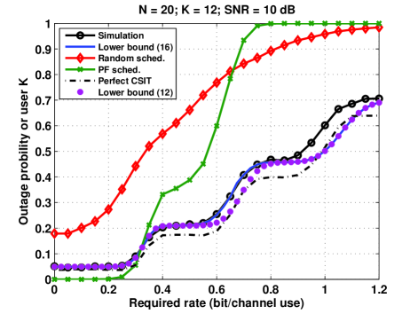
Figure 1: Outage probability with different required rates.

For max-based scheduling, we see that the outage performance is worse with CSIT error. However, the outage degradation is not significant due to relatively small error variance. The outage performance also displays staircase-like curves. We can attribute each step to the rate range that certain number of transmission slots can support. For example, the lowest rate range is supported when one or more slots are selected and the outage probability is approximately equal to the probability that zero slot is selected.

We also compare the results of max-based scheduling with simulation results of random and PF scheduling [3]. Random scheduler performs much worse than max-based one. For PF scheduling, the user with the largest ratio between the current rate and cumulative rate from past slots is selected to transmit. The performance of PF scheduler is better than that of max-based scheduler for small $R$.

Fig. 2 shows outage probability with variance of CSIT error $\xi^{2}$. We assume that distributions of channel gains of all users are identical, i.e., $\sigma^{2}_{k}=1,\forall k$. With total 12 users ($K=12$), 7 users have perfect CSIT ($\xi^{2}_{k}=0$) while the other 5 users have imperfect CSIT with the same error variance $\xi^{2}$. We note that outage probability of users with CSIT error increases with the error variance. This is due mostly to a decrease in the probability that the user with large error will be selected to transmit. Thus, users with perfect CSIT stand to benefit as we see a decrease in outage.

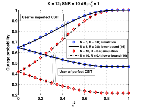
Figure 2: Outage probability for user with either perfect or imperfect CSIT.

VI Conclusions

The derived lower outage bounds are based on union bound and are applicable to max-based scheduling downlink in which user channels are independent Rayleigh fading and may not be identically distributed. The bound is tight for small or moderate required transmission rate or when the number of users is close to or larger than that of time slots. The results show that when CSIT for other users is less accurate, outage performance of user with perfect CSIT improves, and that CSIT error can have serious impact on the outage probability.

[Proof of Proposition 1]

To obtain (25), we first need to determine the conditional probability in the integrand of (15). Recall that $\hat{\gamma}_{K}=|\hat{h}_{K}|^{2}=\hat{h}_{K,r}^{2}+\hat{h}_{K,i}^{2}$ where $\hat{h}_{K,r}$ and $\hat{h}_{K,i}$ are the real and imaginary parts, respectively, of $\hat{h}_{K}$. With (1), the channel power for user $K$ is given by $\gamma_{K}=|h_{K}|^{2}=(\hat{h}_{K,r}+w_{K,r})^{2}+(\hat{h}_{K,i}+w_{K,i})^{2}$ where $w_{K,r}$ and $w_{K,i}$ are real and imaginary parts of $w_{K}$ and are independent Gaussian distributed with zero mean and variance $\frac{1}{2}\xi^{2}_{K}$. Conditioned on $\hat{h}_{K,r}$ and $\hat{h}_{K,i}$, $\gamma_{K}$ is a noncentral Chi-squared random variable with 2 degrees of freedom. Let $\chi^{2}\triangleq\frac{\gamma_{K}}{\frac{1}{2}\xi^{2}_{K}}$ be a normalized noncentral Chi-squared random variable with a noncentrality parameter $\lambda=\frac{2}{\xi^{2}_{K}}(\hat{h}_{K,r}^{2}+\hat{h}_{K,i}^{2})=\frac{2}{\xi^{2}_{K}}x$. Thus,

$$\Pr\bigg{\{}\gamma_{K}<\frac{1}{\rho} (2^{R}-1)\bigg{|}\hat{\gamma}_{K}=x\bigg{\}}$$ (29)

$$=1-\int^{\infty}_{\frac{2}{\xi^{2}_{K}\rho}(2^{R}-1)}f_{\chi^{2}}(z;\frac{2}{\xi^{2}_{K}}x)\,\mathrm{d}z$$ (30)

$$=1-Q_{1}\left(\frac{1}{\xi_{K}}\sqrt{2x},\frac{1}{\xi_{K}}\sqrt{\frac{2}{\rho}(2^{R}-1)}\right).$$ (31)

where the pdf of $\chi^{2}$ is given by

$$f_{\chi^{2}}(z;\lambda)=\frac{1}{2}\mathrm{e}^{-\frac{z+\lambda}{2}}I_{0}(\sqrt{\lambda z}),$$ (32)

and $I_{0}(\cdot)$ denotes the zeroth-order modified Bessel function of the first kind. The complementary cdf for $\chi^{2}$ in (30) can be expressed as the first-order Marcum Q-function defined in [6] as shown in (31).

Finally, to obtain (25), we substitute (31), (23), and (22) into (15), and evaluate the integrals by substituting $y=\sqrt{x}$ and applying the following result, which can be obtained from [7, eqs. (2) and (36)],

$$\int_{0}^{\infty}y\mathrm{e}^{-\frac{1}{2}p^{2}y^{2}}Q_{1}(ay,b)\,\mathrm{d}y=\frac{1}{p^{2}}\mathrm{e}^{-\frac{p^{2}b^{2}}{2(a^{2}+p^{2})}}$$ (33)

where $a$, $b$, and $p$ are constant.

References

• [1] D. J. Love, R. W. Heath, Jr., V. K. N. Lau, D. Gesbert, B. D. Rao, and M. Andrews, “An overview of limited feedback wireless communication systems,” IEEE J. Sel. Areas Commun., vol. 26, no. 8, pp. 1341–1365, Oct. 2008.
• [2] A. Vakili, M. Sharif, and B. Hassibi, “The effect of channel estimation error on the throughput of broadcast channels,” in Proc. IEEE Int. Conf. on Acoustics, Speech and Signal Processing (ICASSP), vol. 4, Toulouse, France, May 2006, pp. IV–IV.
• [3] R. Fritzsche, P. Rost, and G. P. Fettweis, “Robust rate adaptation and proportional fair scheduling with imperfect CSI,” IEEE Trans. Wireless Commun., vol. 14, no. 8, pp. 4417–4427, Aug. 2015.
• [4] S. Guharoy and N. B. Mehta, “Joint evaluation of channel feedback schemes, rate adaptation, and scheduling in OFDMA downlinks with feedback delays,” IEEE Trans. Veh. Technol., vol. 62, no. 4, pp. 1719–1731, May 2013.
• [5] J. Gonter, N. Goertz, and A. Winkelbauer, “Analytical outage probability for max-based schedulers in delay-constrained applications,” in Proc. Wireless Days 2012, Dublin, Ireland, Nov. 2012.
• [6] A. H. Nuttall, “Some integrals involving the ${Q}_{M}$ function,” IEEE Trans. Inf. Theory, vol. 21, no. 1, pp. 95–96, Jan. 1975.
• [7] ——, “Some integrals involving the ${Q}$ function,” Naval Underwater Systems Center, New London, Connecticut, USA, Technical Report 4755, Apr. 1972.