Critical behavior of the spin-$1/2$ Baxter-Wu model: Entropic sampling simulations

Abstract

In this work we use a refined entropic sampling technique based on the Wang-Landau method to study the spin-$1/2$ Baxter-Wu model. The static critical exponents were determined as $\alpha=0.6545(68)$, $\beta=0.0818(30)$, $\gamma=1.18193(77)$, and $\nu=0.66341(47)$. The estimate for the critical temperature was $T_{c}=2.269194(45)$. We compare the present results with those obtained from other well established approaches and we find a very good closeness with the exact values, besides the high precision reached for the critical temperature. We also calculate the coefficients $a$ and $b$ for the divergence of the microcanonical inverse temperature at the ground state achieving an excellent agreement in comparison with the simulation estimates.

I Introduction

In the last decade of the $20^{th}$ century, many researchers contributed to the construction of a new way of performing Monte Carlo simulations without fixing the temperature as it is done in the Metropolis method. Good reasons for this trend were to avoid the critical slowing down in second order phase transitions and to overcome the tunneling barrier between coexisting phases at the transition temperature in first order phase transitions. To mention a few efforts in this direction, there is the multicanonical methodberg1 ; berg2 ; berg3 ; janke , the entropic sampling methodlee (today it is usual to refer to all the methods that estimate $\ln g(E)$, where $g(E)$ is the density of states, as entropic sampling methods), and the broad histogram algorithmbroad1 ; broad2 ; broad3 among others. The culmination of this sequence of works was the Wang-Landau algorithmWangLandau2001 which yielded very impressive results in estimating the density of states. Zhou and BhattZhouBhatt2005 demonstrated the convergence of the method, on the other hand Belardinelli and Pereyrabelardinelli have shown that the error saturates much earlier than expected in the original paper. Caparica and Cunha-Nettocaparica proposed some easily implementable changes to the method in order to improve accuracy, such as adopting the Monte Carlo step for updating the density of states and excluding the initial WL simulation levels from the microcanonical averages. In a later paper Caparicacaparica3 proposed a criterion for halting the simulations and demonstrated that the convergence of Ref. ZhouBhatt2005 is not towards the correct value, but tends to a value within a Gaussian distribution. Furthermore it was demonstrated in that work that even taking into account all the improvements proposed in Ref.caparica the final results still fall into a Gaussian distribution and to overcome these difficulties one should perform at least ten independent sets of finite-size scaling simulations.

In the present work we carry out a study of the Baxter-Wu model applying the improved entropic method following Refs. WangLandau2001 ; caparica ; caparica3 combining finite-size scaling and cumulant methods.

The Baxter-Wu (BW) model although less widespread than the Ising model can also be considered a benchmark in statistical physics. It exhibits a second order phase transition and there are exact solutions for the critical temperature and critical exponents. The model was solved by R.J. Baxter and F.Y. Wubw1 ; bw2 ; bw3 . It consists of a two-dimensional triangular lattice with $\sigma_{i}=\pm 1$ spins located in the vertices of the triangles and interacting via a three spin interaction and having the same critical temperature of the Ising model and critical exponents $\alpha=\nu=2/3$, $\beta=1/12$ and $\gamma=7/6$, belonging therefore to the same universality class of the $q=4$ Potts model. This should be intuitively expected, since the BW model has the same symmetry and the same degree of degeneracy in the ground state of the $q=4$ Potts model with four different configurations. Therefore, the BW model is a rich ground for performing and testing simulational methods.

The outline of this paper is as follows: In section II we define the model. In section III we describe the simulation procedure. In section IV we present the finite-size scaling analysis. The results are discussed in section V and we devote section VI to the summary and concluding remarks.

II Baxter-Wu Model

The BW model was initially proposed by D. W. Wood and H. P. Griffithswood in 1972. This model is defined in a triangular two-dimensional lattice, such that a three-spin interaction is given by the Hamiltonian,

$${\cal H}=-J\sum_{<i,j,k>}\sigma_{i}\sigma_{j}\sigma_{k},$$ (1)

where the spin variables are located at the vertices of the lattice and take the values $\sigma_{i}=\pm 1$, $J$ is the coupling constant that defines the energy scale and the sum extends over all triangular faces of the lattice. One of the reasons that motivated the construction of this model was the elaboration of a magnetic model in which there is no symmetry by inversion of spins and that exhibits an order-disorder transition.

The triangular lattice can be divided into three sub-lattices A, B, C, as represented in top of Fig.1, so that any triangular face (i, j, k) contains one site of type A, one of type B, and one of type C.

Figure 1: (color online). Top: Representation of the Baxter-Wu model as a superposition of three sub-lattices on a triangular lattice. Bottom: Transposition of the triangular lattice to a square lattice.

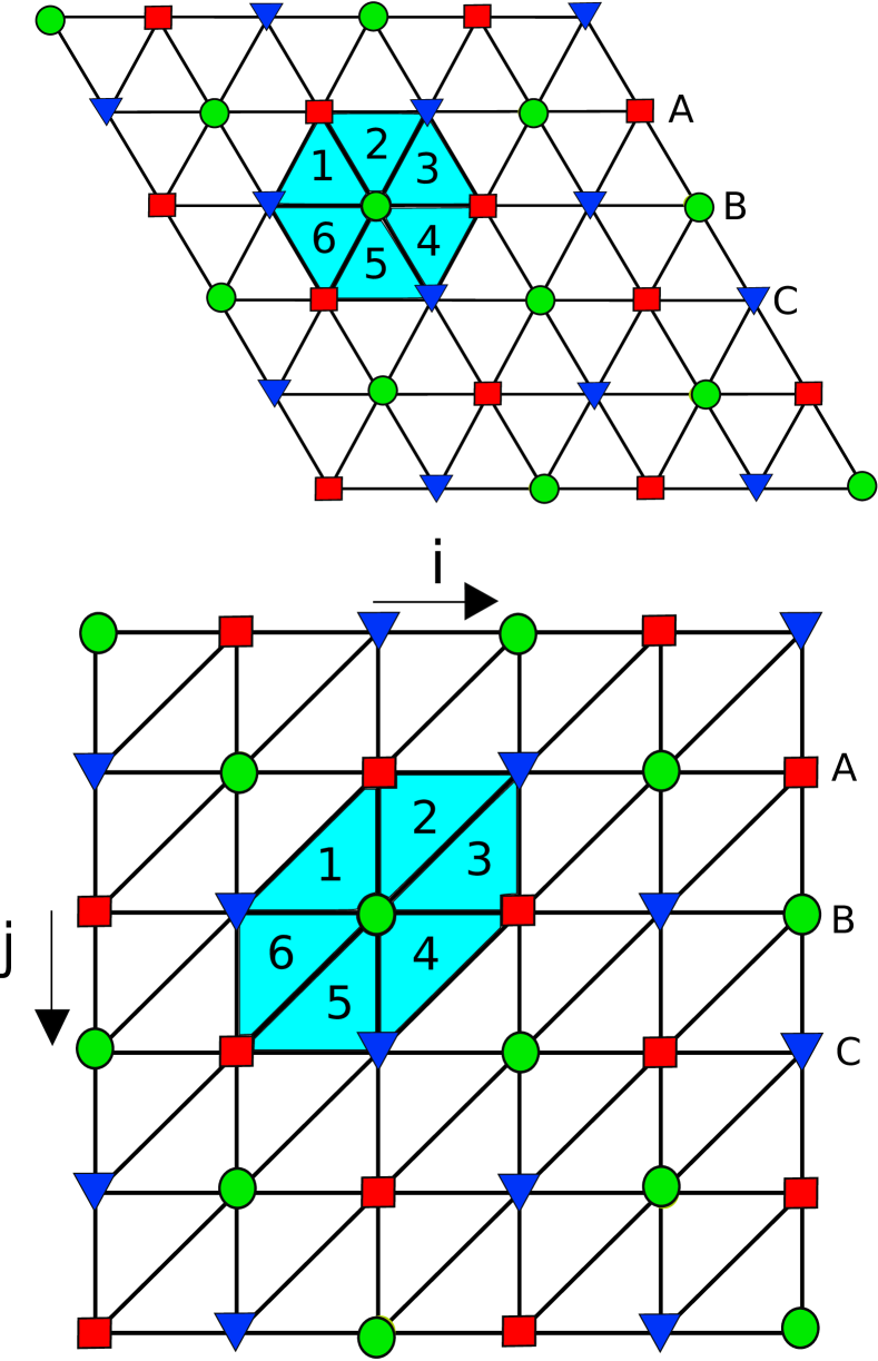
The model exhibits four distinct ground state configurations, namely one with all spins positive and still other three where the spins of two sub-lattices are negated successively.

The configurations on the triangular lattice may be transposed to isomorphic configurations on a square lattice as shown in bottom of Fig.1. One can therefore deal with the model considering spins $\sigma_{i}\equiv s_{ij}$ on a square lattice, using periodic boundary conditions. Each spin is surrounded by six triangular faces, as shown in Fig.1. If one runs all the spins of the configuration counting six faces for each spin, each triangular face will be considered three times. Therefore, the energy of a given configuration of lattice size $L$ defined by the Hamiltonian (1) can be calculated in the square lattice as

$$E= -\frac{J}{3}\sum_{i=1}^{L}\sum_{j=1}^{L}s_{i,j}(s_{i-1,j}s_{i,j-1}+s_{i,j-1}s_{i+1,j-1}$$

$$+s_{i+1,j-1}s_{i+1,j}+s_{i+1,j}s_{i,j+1}+s_{i,j+1}s_{i-1,j+1}$$

$$+s_{i-1,j+1}s_{i-1,j})$$ (2)

Our simulations were performed using this square lattice scheme.

III Entropic Sampling Simulations

The seminal idea of the Wang-Landau method WangLandau2001 is that a random walk in the energy space with a probability proportional to the inverse of the density of states generates a flat histogram for the energy distribution. In fact one estimates $S(E)\equiv\ln g(E)$, because estimating the density of states $g(E)$ would produce huge numbers. The simulation begins setting initially $S(E)=0$ for all energy levels. The random walk in the energy space runs through the energy levels with a probability $p(E\rightarrow E^{\prime})=\min(\frac{g(E)}{g(E^{\prime})},1)$, where $E$ and $E^{\prime}$ are the energies of the current and the next possible configurations, respectively. If a configuration is accepted we update $H(E^{\prime})\rightarrow H(E^{\prime})+1$ and $S(E^{\prime})\rightarrow S(E^{\prime})+F_{i}$, where $F_{i}=\ln f_{i}$, $f_{0}\equiv e=2.71828...$ and $f_{i+1}=\sqrt{f_{i}}$, where $f_{i}$ is defined in the method as the modification factor. After a number of Monte Carlo steps (MCS) we check the histogram for flatness and usually we consider the histogram flat if $H(E)>0.8\langle H\rangle$, for all energies, where $\langle H\rangle$ is an average over the energies. If the flatness condition is satisfied, the modification factor is updated to a finer one and the histogram is reseted $H(E)=0$.

Recently some small changes in this procedure were proposed caparica ; caparica3 ; caparica1 ; caparica2 . Namely (i) the density of states should be updated only after each Monte Carlo sweepmcs , since it avoids taking into account highly correlated configurations when estimating the density of states; (ii) the simulations should be carried out only up to $\ln f=\ln f_{final}$ defined by the canonical averages during the simulations. In this case we save CPU time, discarding superfluous long simulations; and (iii) the initial WL levels should be neglected before accumulating the microcanonical averages, because the configurations in the beginning of the simulations do not match those of maximum entropy. The adoption of these easily implementable modifications leads to more accurate results and saves computational time. They investigated the behavior of the maxima of the specific heat

$$C(T)=\langle(E-\langle E\rangle)^{2}\rangle/T^{2}$$ (3)

and the magnetic susceptibility

$$\chi(T)=L^{2}\langle(m-\langle m\rangle)^{2}\rangle/T,$$ (4)

where $E$ is the energy of a given configuration and $m$ is the corresponding magnetization per spin, during the WL sampling for the Ising model on a square lattice. They demonstrated that a substantial part of the conventional Wang-Landau simulation is not necessary because the error saturates. They observed that in general no single simulation run converges to the real value of any physical quantity, but to a particular value of a Gaussian distribution of results around the true value. The saturation of the error matches with the convergence to this value. Simulations beyond this limit leads to negligible variations in the canonical averages of all thermodynamic variables.

Another innovation proposed in Ref.caparica3 is a criterion for halting the simulations. During the WL sampling of a given model, beginning from $f_{5}$, one calculates the temperature of the peak of the specific heat defined in Eq. (3) using the current $g(E)$ and from then on this mean value is updated whenever the histogram is checked for flatness. If the histogram is considered flat, we save the value of the temperature $T_{c}(0)$ of the peak of the specific heat. During the simulations with the new modification factor the temperature of the peak of the specific heat $T_{c}(t)$ continues being calculated when the histogram is checked for flatness along with the checking parameter

$$\varepsilon=|T_{c}(t)-T_{c}(0)|.$$ (5)

If the number of MCS before verifying the histogram for flatness is not too large, then during the simulations with each modification factor the checking parameter $\varepsilon$ is computed multiple times. If $\varepsilon$ remains below $10^{-4}$ up until the histogram meets the flatness criterion for this WL level, then one should save the density of states and the microcanonical averages and stop the simulations. When we adopt this criterion for halting the simulations, the final modification factors may be different for different runs.

Once obtained the density of states, one can calculate the canonical average of any thermodynamic variable $X$ as

$$\langle X\rangle_{T}=\dfrac{\sum_{E}\langle X\rangle_{E}g(E)e^{-\beta E}}{\sum_{E}g(E)e^{-\beta E}},$$ (6)

where $\langle X\rangle_{E}$ is the microcanonical average accumulated during the simulations and $\beta=1/k_{B}T$, where $T$ is the absolute temperature measured in units of $J/k_{B}$ and $k_{B}$ is the Boltzman’s constant.

It was also observed in Ref.caparica3 that two independent similar finite-size scaling procedures can lead to quite different results for the exponents and the critical temperature, which in general do not agree within the error bars. The way to circumvent this problem is to carry out 10 independent sets of finite-size scaling simulations. In this work, for each of these sets we perform simulations for $L=32,40,44,52,56,64,76,$ and $80$ with $n=24,20,20,16,16,16,12,$ and $12$ independent runs for each size, respectively. The final resulting values for the critical temperature and the critical exponents are obtained as an average over all sets.

IV Finite-size scaling

From the definition of the free energy, according to finite-size scaling theory fisher1 ; fisher2 ; barber , one can obtain the zero field scaling expressions for the magnetization, susceptibility, and specific heat, respectively, by

$$m\approx L^{-\beta/\nu}\mathcal{M}(tL^{1/\nu}),$$ (7)

$$\chi\approx L^{\gamma/\nu}\mathcal{X}(tL^{1/\nu}).$$ (8)

$$c\approx c_{\infty}+L^{\alpha/\nu}\mathcal{C}(tL^{1/\nu}),$$ (9)

where $t=(T_{c}-T)/T_{c}$ is the reduced temperature, and $\alpha$, $\beta$, and $\gamma$ are static critical exponents which should satisfy the scaling relation privman

$$2-\alpha=d\nu=2\beta+\gamma.$$ (10)

According to Refs. chen1993 ; double we can define a set of thermodynamic quantities defined as functions of logarithmic derivatives of the magnetization:

$$V_{1} \equiv 4[m^{3}]-3[m^{4}],$$ (11)

$$V_{2} \equiv 2[m^{2}]-[m^{4}],$$ (12)

$$V_{3} \equiv 3[m^{2}]-2[m^{3}],$$ (13)

$$V_{4} \equiv(4[m]-[m^{4}])/3,$$ (14)

$$V_{5} \equiv(3[m]-[m^{3}])/2,$$ (15)

$$V_{6} \equiv 2[m]-[m^{2}],$$ (16)

where

$$[m^{n}]\equiv\ln\frac{\partial\langle m^{n}\rangle}{\partial T}.$$ (17)

Using these thermodynamic quantities one can determine the static critical exponent $\nu$ , even not having yet an estimate for the critical temperature, since taking into account Eq. (7) it is simple to show that

$$V_{j}\approx\frac{1}{\nu}\ln L+\mathcal{V}_{j}(tL^{1/\nu})$$ (18)

for $j=1,2,...,6.$ At the critical temperature $T_{c}$ ($t=0$) the $\mathcal{V}_{j}$ are constants not dependent of the system size $L$. Having an estimate for the critical exponent $\nu$ it is possible to determine the critical temperature. According to Eqs. (8) and (9) locations of the extrema of the specific heat and the susceptibility, Eqs. (3) and (4), vary asymptotically as

$$T_{c}(L)\approx T_{c}+a_{q}L^{-1/\nu},$$ (19)

where $a_{q}$ is a quantity-dependent constant, enabling then the determination of $T_{c}$. And then, with the exponent $\nu$ and $T_{c}$ at hand, we can calculate the exponents $\beta$ and $\gamma$ by the slopes of the log-log plots of Eqs. (7) and (8) evaluated at the critical temperature $T_{c}$.

V Results

V.1 The critical exponents and the critical temperature

We carried out the simulations adopting the MCS for updating the density of states and the microcanonical averages were accumulated beginning from $f_{7}$. The jobs were halted using the checking parameter $\varepsilon$.

Figure 2: (color online). Top: Evolution of the temperature of the maximum of the specific heat during the WL sampling, beginning from $f_{9}$ for a single run. The dots show where the modification factor was updated. Bottom: Evolution of the logarithm of the checking parameter $\varepsilon$ during the same simulation.

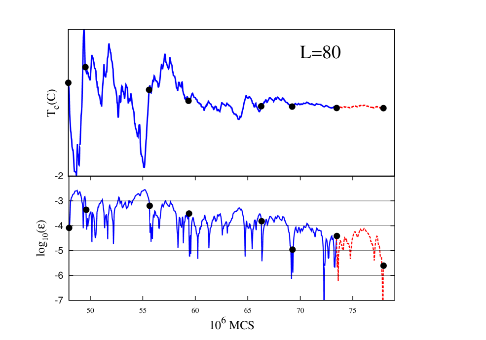
In Fig.2 we show the dependence of the temperature of the maximum of the specific heat during the WL sampling with the number of MC steps (MCS), beginning from $f_{9}$ for a single run with $L=80$ and the evolution of log${}_{10}(\varepsilon)$ during the same simulation. At the last WL level the logarithm of $\varepsilon$ remains below $-4$ indicating that the simulation can be halted at the end of $f_{15}$.

Figure 3: (color online) Size dependence of the maxima of $V_{j}$. The slopes yield $1/\nu$.

Figure 4: (color online) Size dependence of the locations of the extrema in the specific heat and the susceptibility with $\nu=0.66341$.

Figure 5: (color online) Log-log plot of the size dependence of the finite-lattice magnetization at $T_{c}=2.269194$.

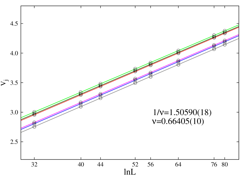
By locating the extrema of the thermodynamic functions defined in Eqs. (11)-(16) we can determine the critical exponent $\nu$ as the inverse of the slopes of the straight lines given by Eq. (18), since at $T_{c}$ ($t=0$) the $\mathcal{V}_{j}$ should be constants independent of the system size $L$. In Fig. 3 we present this set of lines. For each of these six slopes we calculate $\nu=1/(\frac{1}{\nu})$ with $\varDelta\nu=\varDelta(\frac{1}{\nu})/(\frac{1}{\nu})^{2}$ and take an average with unequal uncertainties wong over them. From the linear fits to these points we estimate $\frac{1}{\nu}=1.50590(18)$, yielding ${\nu}=0.66405(10)$. Notwithstanding these values represent the result of only one of the $10$ sets of finite-size scaling simulations which were performed. Initially we run over all folders calculating $\nu$ in order to determine this exponent to the best precision. As in Refs. potts ; dsde to calculate the mean value of these ten results we adopted a single averaging instead of an average with unequal uncertainties, since the values fall into a Gaussian distribution and in most cases they do not agree within the error bars. Thus,performing the second procedure would lead to an unrealistic small error bar. In the first column of Table 1 we display the results for this exponent in each set and the final average at the last line yielding $\nu=0.66341(47)$. An additional discussion on the way we are taking these averages could be held taking into account Ref. weigel . In this work the authors propose a formulation using the cross correlations, as is the situation of our six estimates for calculating the exponent $\nu$. They assert that the resulting average with unequal uncertainties remains a valid estimator and only the error bars would be modified by the new formulation. But in our case the error bars obtained in each set are neglected when we take the final average. Moreover in the references of this work they include the following comment: “Note that when using the Wang-Landau method as a direct estimate of the density of states to be used for computing thermal expectation values, due to the non-Markovian nature of the algorithm there is currently no known approach of reliably estimating the present statistical fluctuations apart from repeating the whole calculation a certain number of times.”

Figure 6: (color online) Log-log plot of the size dependence of the finite-lattice susceptibility at $T_{c}=2.269194$.

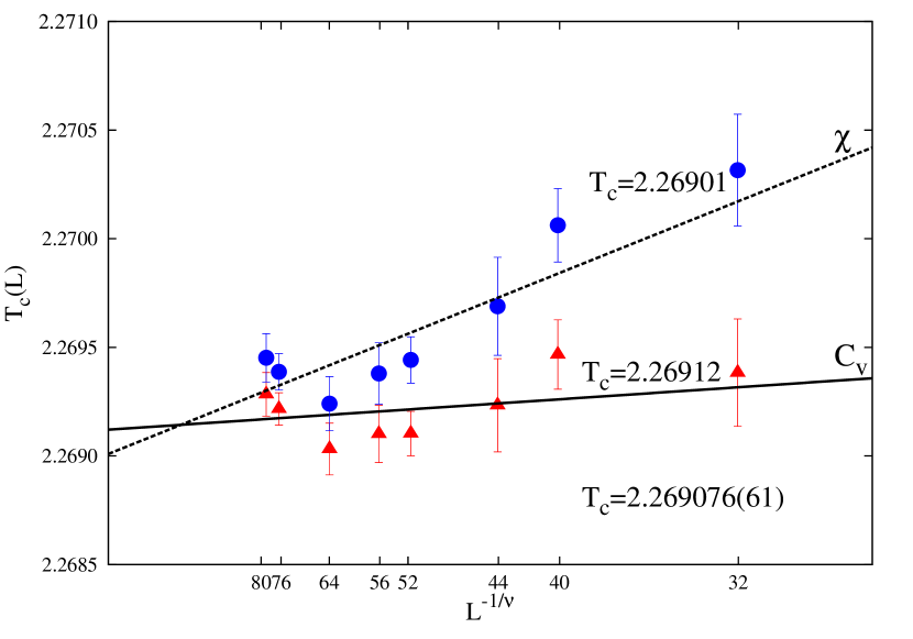
With the critical exponent $\nu$ accurately determined we can use Eq. (19) to determine $T_{c}$ as the extrapolation to $L\rightarrow\infty$ ($L^{-1/\nu}=0$) of the linear fits given by the locations of the maxima of the specific heat and the susceptibility defined by Eqs. (3) and (4). In Fig. 4 we show these linear fits that converge to $T_{c}$ at $L^{-1/\nu}=0$. At first glance the pattern seems to be disappointing with the points badly aligned and with large error bars, but in fact this is because all the results are unusually close to the correct value. The final numerical extrapolations are therefore excellent. In the second column of Table 1 we display the results for the critical temperature obtained in each set and at the last line the mean value giving $T_{c}=2.269194(45)$.

$\nu$	$T_{c}$	$\beta$	$\gamma$
0.66405(20)	2.269076(86)	0.0926(78)	1.1850(34)
0.66553(64)	2.26938(10)	0.0690(95)	1.1762(38)
0.66242(67)	2.269189(85)	0.0821(72)	1.1822(39)
0.66150(41)	2.269162(75)	0.0816(73)	1.1835(28)
0.66139(42)	2.26899(11)	0.093(10)	1.1851(31)
0.66276(56)	2.26924(13)	0.083(11)	1.1845(40)
0.66353(43)	2.269329(75)	0.0705(71)	1.1795(26)
0.66498(63)	2.26905(11)	0.0905(90)	1.1819(34)
0.66522(68)	2.26912(11)	0.0867(89)	1.1808(36)
0.66271(47)	2.269410(99)	0.0694(99)	1.1806(41)
0.66341(47)	2.269194(45)	0.0818(30)	1.1819(17)

Table 1: Ten finite size scaling results for the critical temperature $T_{c}$, and the exponents $\nu$, $\beta$ and $\gamma$. The average over all runs are shown at the last line.

Method	$\alpha$	$\beta$	$\gamma$	$\nu$
$q=4$ Potts model
Conjectured values Wu1982	$\frac{2}{3}\cong 0.667$	$\frac{1}{12}\cong 0.083$	$\frac{7}{6}\cong 1.167$	$\frac{2}{3}\cong 0.667$
Kadanoff variational RG dasgupta	$0.488$	$0.091$	$1.330$	$0.756$
Duality invariant RG hu	$0.4870$	$-$	$-$	$0.7565$
Critical dynamics alternative	$-$	$0.0835(4)$	$-$	$0.669(6)$
Entropic sampling potts	$0.5084(48)$	$0.0877(37)$	$1.3161(69)$	$0.7076(10)$
Baxter-Wu model
Exact solution baxter	$\frac{2}{3}\cong 0.667$	$\frac{1}{12}\cong 0.083$	$\frac{7}{6}\cong 1.167$	$\frac{2}{3}\cong 0.667$
Critical dynamics wagner	$-$	$0.0817(23)$	$-$	$0.621(9)$
Critical dynamics everaldo	$-$	$0.080(2)$	$-$	$0.67(1)$
This work	$0.6545(77)$	$0.0818(30)$	$1.1819(17)$	$0.66341(47)$

Table 2: Estimates of $\alpha$, $\beta$, $\gamma$, and $\nu$ compared to results obtained with other techniques, conjectured, and exact values.

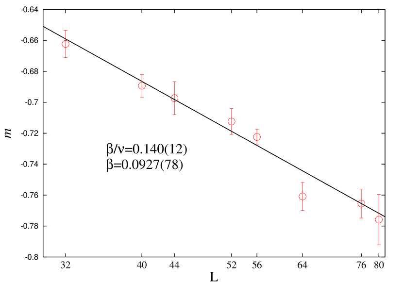
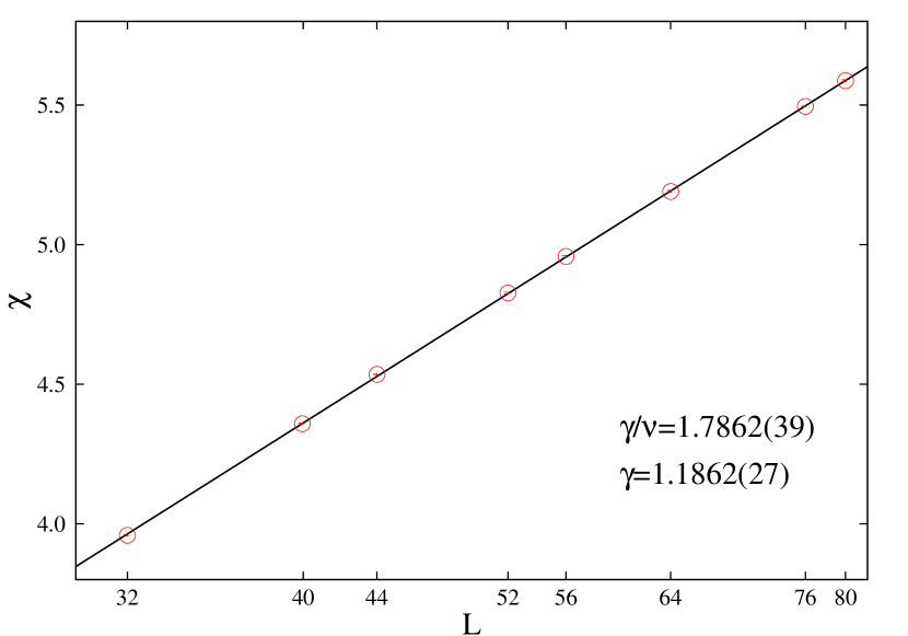
Next, with the critical temperature $T_{c}$ and the critical exponent $\nu$ estimated to a high precision, we can use Eqs.(7)-(8) to determine the exponents $\frac{\beta}{\nu}$ and $\frac{\gamma}{\nu}$ by the slopes of the log-log plots. Fig. 5 and Fig. 6 show this finite-size scaling behavior for each exponent, yielding $\frac{\beta}{\nu}=0.140(12)$ and $\frac{\gamma}{\nu}=1.7862(39)$, respectively. We then estimate $\beta=\nu\frac{\beta}{\nu}$ with $\varDelta\beta=\frac{\beta}{\nu}\varDelta\nu+\nu\varDelta\frac{\beta}{\nu}$, and similarly for $\gamma$ and $\varDelta\gamma$, obtaining $\beta=0.0926(78)$, and $\gamma=1.1850(34)$. Over again, these values are calculated at the first set. In the two last columns of Table 1 we show the results for all folders and the best estimates at the last line, obtaining $\beta=0.0818(30)$, and $\gamma=1.1819(17)$. As a final result, using the scaling relation given by Eq. (10) we can calculate the exponent $\alpha=2-2\beta-\gamma$ with $\varDelta\alpha=2\varDelta\beta+\varDelta\gamma$ giving $\alpha=0.6545(77)$.

In Table 2 we compare our final estimates of the critical exponents to other well-established values. It is noteworthy the proximity of our estimates of the critical exponents with the exact values. The good resolution we have obtained in this study corroborates the strength of the adopted technique.

V.2 The $a$ and $b$ coefficients of the divergence of the microcanonical inverse temperature

The microcanonical inverse temperature is defined as

$$\frac{1}{T}=\frac{\partial S}{\partial E}=\lim_{\varDelta E\to 0}\frac{\varDelta S}{\varDelta E}.$$ (20)

In the ground state this limit should be infinity. Nevertheless for any discrete model, as in the Baxter-Wu model, $\varDelta E=const$. Therefore the limit becomes exact only if $L\rightarrow\infty$ ($E_{min}\rightarrow-\infty$), where $L$ is the linear lattice size dsde .

Figure 7: (Color online) Size dependence of $\frac{\varDelta S}{\varDelta E}$ at the ground state of the first set of simulations. The line is the best fitting curve of these data to $a\ln(bL)$. The error bars are smaller than the symbols.

$a$	$b$
0.16680(10)	0.9972(16)
0.16714(12)	0.9897(25)
0.16692(10)	0.9946(20)
0.16701(11)	0.9928(23)
0.16659(16)	1.0028(34)
0.16663(11)	1.0006(24)
0.16621(10)	1.0100(21)
0.16669(11)	0.9988(25)
0.16646(10)	1.0052(20)
0.16663(10)	1.0001(20)
0.166707(86)	0.9992(19)

Table 3: Estimates by entropic sampling simulations of the parameters $a$ and $b$ for the Baxter-Wu model.

In the Baxter-Wu model the ground state has four configurations, one with all spins positive and three more where two sub-lattices are negated successively. If a single spin is flipped, it looses six negative links from the neighboring triangular faces and gains six positive ones. The energy gap between the ground state and the next state is therefore $\varDelta E=6-(-6)=12$, where we take the coupling constant $J$ as 1. The first higher level has $4L^{2}$ configurations yielding $\varDelta S=\ln 4+2\ln L-\ln 4$ and, since $\varDelta E=12$, we have

$$\frac{\varDelta S}{\varDelta E}=\frac{1}{6}\ln L\cong 0.1667\ln L.$$ (21)

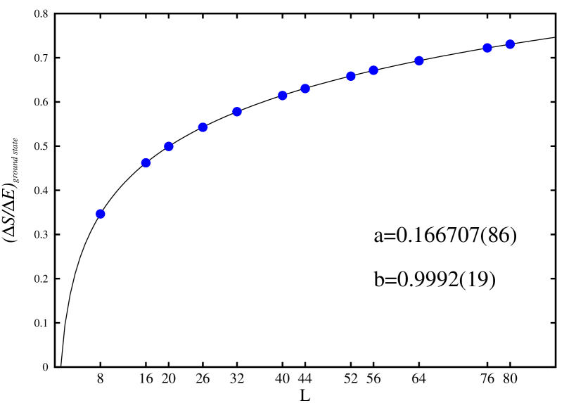
For notational simplicity we set $k_{B}=1$. Just as in the cases discussed in Ref. dsde the inverse temperature of the Baxter-Wu model diverges in the ground state as $a\ln(bL)$, yielding $a=\frac{1}{6}$ and $b=1$. For estimating the coefficients $a$ and $b$ from our simulational data we added four smaller sizes, $L=8,16,20,26$. In Fig. 7 we show the dependence of $\frac{\varDelta S}{\varDelta E}$ at the ground state on the lattice sizes using the outcomes of the first set of simulations, along with the best fitting curve to $a\ln(bL)$. The agreement is excellent. In Table 3 we display the values obtained in our entropic simulations for $a$ and $b$. The ten initial lines correspond to results obtained in each set and the last line is a single average over all sets neglecting the error bars. One can see that we get very accurate results for $a$ and $b$, which agree within error bars equal to $\pm 1\sigma$ with the exact coefficients $a=\frac{1}{6}$ and $b=1$.

VI Conclusions

We carried out a high-resolution study of the static critical behavior of the Baxter-Wu model using a refined entropic sampling procedure based on the Wang-Landau method. Our results present an impressive agreement with the exact values for the critical exponents and with the critical temperature as well. Such upshot corroborates the correctness of the improvements suggested to the original Wang-Landau sampling. Finally we calculated the exact values for the recently proposed coefficients $a$ and $b$ for the divergence of the microcanonical inverse temperature in the ground state and we also obtained an excellent concordance of the simulation estimates with them.

VII Acknowledgment

We acknowledge the computer resources provided by LCC-UFG and IF-UFMT. L. N. Jorge acknowledges the support by FAPEG.

References

- (1) R. J. Baxter and F.Y. Wu, Phys. Rev. Lett. 31, 1294 (1973).
- (2) R. J. Baxter and F.Y. Wu, Aust. J. Phys. 27, 357 (1974).
- (3) R. J. Baxter, Aust. J. Phys. 27, 368 (1974).
- (4) B. A. Berg and T. Neuhaus, Phys. Rev. Lett. 68, 9 (1992).
- (5) B. A. Berg and T. Celik, Phys. Rev. Lett. 69, 2292 (1992).
- (6) B. A. Berg, U. Hansmann, and T. Neuhaus, Phys. Rev. B 47, 497 (1993).
- (7) W. Janke and S. Kappler, Phys. Rev. Lett. 74, 212 1995.
- (8) J. Lee, Phys. Rev. Lett. 71, 211 (1993).
- (9) P. M. C. Oliveira, T. J. P. Penna, and H. J. Herrmann, Braz. J. Phys. 26, 677 (1996).
- (10) P. M. C. Oliveira, T. J. P. Penna, and H. J. Herrmann, Eur. Phys. J. B 1, 205 (1998).
- (11) P. M. C. Oliveira, Eur. Phys. J. B 6, 111 (1998).
- (12) F. Wang and D. P. Landau, Phys. Rev. Lett. 86, 2050 (2001); Phys. Rev. E 64, 056101 (2001).
- (13) C. Zhou and R. N. Bhatt, Phys. Rev. E 72, 025701 (2005).
- (14) R. E. Belardinelli and V. D. Pereyra, J. Chem. Phys. 127, 184105 (2007).
- (15) A.A. Caparica and A.G. Cunha-Netto, Phys. Rev. E 85, 046702 (2012).
- (16) A.A. Caparica, Phys. Rev. E 89, 043301 (2014).
- (17) Wood, D. W. and Griffiths, H.P., J. Phys. C: Solid State Phys. 5, L253-5 (1972).
- (18) L.S. Ferreira and A.A. Caparica, Int. J. Mod. Phys. C 23, 1240012 (2012).
- (19) L.S. Ferreira, A.A. Caparica, M. A. Neto, and M. D. Galiceanu, J. Stat. Mech., 2012, P10028 (2012).
- (20) A Monte Carlo sweep consists of spin-flip trials in the 2D lattice.
- (21) F.Y Wu, The Potts model, Rev. Mod. Phys. 54, 235 (1982).
- (22) M.E. Fisher, in Critical Phenomena, edited by M. S. Green (Academic, New York, 1971).
- (23) M.E. Fisher and M.N. Barber, Phys. Rev. Lett. 28, 1516 (1972).
- (24) Phase Transitions and Critical Phenomena, edited by C. Domb and J. L. Lebowitz (Academic, New York, 1974), Vol. 8.
- (25) V. Privman, P.C. Hohenberg, and A. Aharony, in Phase Transitions and Critical Phenomena, eduted by C. Domb and J. L. Lebowitz (Academic, New York, 1991), Vol. 14, p. 1.
- (26) K. Chen,A.M. Ferrenberg, and D.P. Landau, Phys. Rev. B 48, 3249 (1993).
- (27) A.A. Caparica, A. Bunker, and D.P. Landau, Phys. Rev. B 62, 9458 (2000); There is a misprinting in Eq.(3) in this paper, which should be .
- (28) S.S.M. Wong, Computational Methods in Physics and Engineering, 2nd edition, World Scientific Publishing Co. Pte. Ltd. (1997).
- (29) H. A. Fernandes, E. Arashiro, J. R. Drugowich de Felício, and A. A. Caparica, Physica A 366 255–264 (2006).
- (30) A. A. Caparica, S. A. Leão, and C. J. DaSilva, Physica A 438 447–453 (2015).
- (31) A. A. Caparica, S. A. Leão, and C. J.DaSilva, Braz. J. Phys., DOI 10.1007/s13538-015-0361-8 (2015).
- (32) M. Weigel and W. Janke, Phys. Rev. E 81, 066701 (2010).
- (33) C. Dasgupta, Phys. Rev. B 15, 3460 (1977).
- (34) B. Hu, J. Phys. A 13, L321 (1980).
- (35) R. J. Baxter, Exactly Solved Models in Statistical Mechanics, p. 320, (Academic Press, London, 1982).
- (36) M. Santos and W. Figueiredo, Phys. Rev. E 63, 042101 (2001).
- (37) E. Arashiro and J. R. Drugowich de Felício, Phys. Rev. E 67, 046123 (2003).