Collective Bulk and Edge Modes through the Quantum Phase Transition in Graphene at $\nu=0$

Abstract

Undoped graphene in a strong, tilted magnetic field exhibits a radical change in conduction upon changing the tilt-angle, which can be attributed to a quantum phase transition from a canted antiferromagnetic (CAF) to a ferromagnetic (FM) bulk state at filling factor $\nu=0$. This behavior signifies a change in the nature of the collective ground state and excitations across the transition. Using the time-dependent Hartree-Fock approximation, we study the collective neutral (particle-hole) excitations in the two phases, both in the bulk and on the edge of the system. The CAF has gapless neutral modes in the bulk, whereas the FM state supports only gapped modes in its bulk. At the edge, however, only the FM state supports gapless charge-carrying states. Linear response functions are computed to elucidate their sensitivity to the various modes. The response functions demonstrate that the two phases can be distinguished by the evolution of a local charge pulse at the edge.

I Introduction

Graphene subject to a perpendicular magnetic field exhibits a quantum Hall (QH) state at $\nu=0$. While such a state can exist in the noninteracting model with a Zeeman coupling, the $\nu=0$ state in experimental samples is believed to be driven by electron-electron interactions Zhang_Kim2006 ; Alicea2006 ; Goerbig2006 ; Gusynin2006 ; Nomura2006 ; Herbut2007 ; Jiang2007 ; Fuchs2007 ; Abanin2007 ; Checkelsky ; Du2009 ; Goerbig2011 ; Dean2012 ; Yu2013 . In such a hypothetical interacting state the bulk gap in the half-filled zero Landau level would be associated with the formation of a broken-symmetry many-body state. The variety of different ways to spontaneously break the $SU(4)$ symmetry in spin and valley space suggests an enormous number of potential ground states Herbut2007AF ; Jung2009 ; Nandkishore ; Kharitonov_bulk ; Roy2014 ; Lado2014 ; QHFMGexp .

Recent experiments seem to see two such $\nu=0$ statesYoung2013 ; Maher2013 , with a phase transition between them tuned by changing the Zeeman coupling strength. In these experiments, the perpendicular field $B_{\perp}$ is kept fixed while the Zeeman coupling is tuned by changing the parallel field $B_{\parallel}$. Being at $\nu=0$, both states naturally show $\sigma_{xy}=0$. At low Zeeman coupling, the sample has a vanishing two-terminal conductance, indicating that its state is a “vanilla” insulator, whereas beyond a certain critical Zeeman coupling, the sample has an almost perfect two-terminal conductance of $2e^{2}/h$, suggesting that it is in a quantum spin Hall state with protected edge states.

The most plausible interpretation of these experiments is in view of a theoretical work of Kharitonov Kharitonov_bulk ; bilayer_QHE_CAF , which predicted a $T=0$ quantum phase transition from a canted antiferromagnetic (CAF) (the “vanilla” insulator) to a spin-polarized ferromagnetic (FM) quantum Hall-like state tuned by increasing the Zeeman energy $E_{z}$ to appreciable values. The behavior of the two-terminal conductance is explained by the nature of the edge modesGusynin2008 ; Kharitonov_edge ; Murthy2014 ; Pyatkovskiy2014 ; Knothe2015 ; Takei2015 of the two zero-temperature phases. Previous investigations have shown that the FM state has a fully gapped bulk, but supports gapless, helical, charged excitations at its edge Abanin et al. (2006); Fertig2006 ; SFP ; Paramekanti . In analogy with the quantum spin Hall (QSH) state in two-dimensional topological insulators Kane-Mele ; TIreview , the gapless edge states of the FM state are immune to backscattering by spin-conserving impurities due to their helical nature: right and left movers have opposite spin flavors.

While Kharitonov’s proposal is consistent with the transport experiments, there has been no direct experimental confirmation of the nature of the two phases. In particlar, alternatives, such as a Kekule-distorted phaseKekule , are potential ground states for the low-Zeeman “vanilla” insulator.

One of our motivations in this study is to find physically measurable quantities in both phases, both at the edge and in the bulk, that provide characteristic signatures of each phase. In a previous paperMurthy2014 , the present authors studied an extension of Kharitonov’s model (to include spin-stiffness) in the Hartree-Fock (HF) approximation. We showed, using a simple model of the edge, that a domain wall is formed near the edge. This domain wall entangles the spin and valley degrees of freedom, and leads to a single-particle spectrum which is gapped everywhere. In the bulk of the FM state, the spins in both valleys are polarized along the total field, which we will call $\uparrow$ for convenience. Deep into the edge, the state must have vacuum quantum numbers, and so must be a singlet. The domain wall is the region where the spin rotates continuously from being fully polarized to being a singlet, thus acquiring an $XY$-component in spin space. At the level of HF, this appears as a spontaneous broken symmetry and an order parameter. Fluctuations about HF will restore the symmetry in accordance with the Mermin-Wagner theorem.

In the FM phase, the low-energy charged excitations of the system are gapless collective modes associated with a $2\pi$ twist of the ground-state spin configuration in the $XY$-planeFertig2006 ; Murthy2014 . This spin twist is imposed upon the position-dependent $S_{z}$ associated with the DW, thus creating a spin texture, with an associated charge that is inherent to QH ferromagnets QHFM ; Fertig1994 . Gapless 1D modes associated with fluctuations of the DW (which can be modeled as a helical Luttinger liquid SFP ) carry charge and contribute to electric conduction. In contrast, the CAF phase is characterized by a gap to charged excitations on the edge Gusynin2008 ; Kharitonov_edge , and a broken $U(1)$ symmetry in the bulk (associated with $XY$-like order parameter) implying a neutral, gapless bulk Goldstone mode. As we have shown in our earlier work Murthy2014 , a proper description of the lowest energy charged excitations of this state involves a coupling between topological structures at the edge and in the bulk, associated with the broken $U(1)$ symmetry.

In this paper we will carry forward our previous analysis, and focus on the behavior of the collective particle-hole excitations in both phases, which we compute in the time-dependent Hartree-Fock (TDHF) approximation. Our goal is three-fold: Firstly, we want to verify that the charged edge modes we proposed in previous work can be seen in particle-hole excitations as well. Secondly, we will find experimental signatures of the two different phases in the bulk as well as at the edge. Thirdly, we want to compute a set of parameters that we can use to build an effective theory of the edge.

The plan of this paper is as follows: In Section II we will define our notational conventions and review the HF calculation of our previous work. In Section III we will present the TDHF formalism and general expressions for the spectral densities of various correlation functions. In Section IV we will present our results, giving particular emphasis to the experimental signatures of the bulk and edge collective modes. We end with conclusions and discussion in Section V.

II Hamiltonian and Hartree-Fock Approximation

We start with some notational conventions. In the $n=0$ Landau level of graphene, there are two spin (${\uparrow}$ and ${\downarrow}$) and two valley ($K$ and $K^{\prime}$) degrees of freedom. In Landau gauge, we can label the orbital part of the single-particle states by $X=kl^{2}$, where $k$ is the wavevector in the $y$-direction. We order our four-component fermion destruction operators as $\vec{\bf c}_{k}=({\bf c}_{K{\uparrow},k},{\bf c}_{K{\downarrow},k},{\bf c}_{K^{\prime}{\uparrow},k},{\bf c}_{K^{\prime}{\downarrow},k})^{T}$. (Note that throughout this paper, operator quantities are indicated by boldface type.) We define Pauli matrices $\mathbf{\sigma}$ acting in the spin space and $\mathbf{\tau}$ acting in the valley space with $\sigma_{0}=\tau_{0}=I$ (the identity matrix), and define $\ell=\sqrt{\frac{\hbar}{eB_{\perp}}}$ as the magnetic length. With these notations the Hamiltonian (first proposed by Kharitonov Kharitonov_bulk ) becomes

$${\mathbf{H}}=\frac{\pi\ell^{2}}{L^{2}}\sum\limits_{k_{1},k_{2},{\vec{q}}}\sum\limits_{a=0,x,y,z}e^{-\frac{(q\ell)^{2}}{2}}e^{i(\Phi(k_{1},{\vec{q}})+\Phi(k_{2},-{\vec{q}})}:g_{a}\vec{{\mathbf{c}}}^{\,\dagger}_{k_{1}-q_{y}}\tau_{a}\vec{{\mathbf{c}}}_{k_{1}}\vec{{\mathbf{c}}}^{\,\dagger}_{k_{2}+q_{y}}\tau_{a}\vec{{\mathbf{c}}}_{k_{2}}:-\sum_{k}U_{e}(k)\vec{{\mathbf{c}}}^{\dagger}_{k}\tau_{x}\vec{{\mathbf{c}}}_{k}-E_{Z}\sum_{k}\vec{{\mathbf{c}}}^{\,\dagger}_{k}\sigma_{z}\vec{{\mathbf{c}}}_{k},$$ (1)

where $L$ is the linear size of the system and $\Phi(k,{\vec{q}})=\ell^{2}(-q_{x}k-\frac{1}{2}q_{x}q_{y})$.

Note that the SU(4) symmetric $g_{0}$ term in the model does not affect the groundstate phase of the system, and was not included in Ref. Kharitonov_bulk, . It is added here to simulate the spin/valley stiffness that we expect from the long-range Coulomb interaction. We have followed the common device of modelling the edge as a smooth potential that couples to $\tau_{x}$, forcing the ground state to be an eigenstate of $\tau_{x}$ deep inside the edge. Furthermore, $g_{x}=g_{y}\equiv g_{xy}<0$, and $g_{z}>|g_{xy}|$ as required for the system to be in the CAF or FM groundstates. Throughout this paper we will present results for the representative values $g_{0}=5$, $g_{z}=0.5$, $g_{xy}=-0.1$. We have checked that other values do not qualitatively alter the results.

In previous work Murthy2014 , we carried out a numerical static HF study, allowing all possible one-body expectation values Murthy2014 . The results can be expressed as follows: The HF single-particle states in the lowest Landau level (LLL) are entangled combinations of spin and valley characterized by two angles we label $\psi_{a}$ and $\psi_{b}$. In the bulk these angles are equal to each other and constant, but near the edge they differ from each other and vary with $k$. The states may be parameterized in the form

$$|a\rangle= \frac{1}{\sqrt{2}}\big{(}\cos{\frac{\psi_{a}}{2}},-\sin{\frac{\psi_{a}}{2}},\cos{\frac{\psi_{a}}{2}},\sin{\frac{\psi_{a}}{2}}\big{)}^{T},$$

$$|b\rangle= \frac{1}{\sqrt{2}}\big{(}-\cos{\frac{\psi_{b}}{2}},\sin{\frac{\psi_{b}}{2}},\cos{\frac{\psi_{b}}{2}},\sin{\frac{\psi_{b}}{2}}\big{)}^{T},$$

$$|c\rangle= \frac{1}{\sqrt{2}}\big{(}\sin{\frac{\psi_{a}}{2}},\cos{\frac{\psi_{a}}{2}},\sin{\frac{\psi_{a}}{2}},-\cos{\frac{\psi_{a}}{2}}\big{)}^{T},$$

$$|d\rangle= \frac{1}{\sqrt{2}}\big{(}\sin{\frac{\psi_{b}}{2}},\cos{\frac{\psi_{b}}{2}},-\sin{\frac{\psi_{b}}{2}},\cos{\frac{\psi_{b}}{2}}\big{)}^{T}.$$ (2)

Defining ${g_{\perp}}=|g_{xy}|$, in the bulk the values of $\psi_{a}=\psi_{b}=\psi$ are given by $\cos{\psi}=\frac{E_{Z}}{2{g_{\perp}}}$ for $E_{Z}<E_{Zc}$, while $\psi=0$ for $E_{Z}>E_{Zc}$. The quantum phase transition occurs at $E_{Zc}=2{g_{\perp}}=0.2$ in our units. Fig. 1 shows the variation of these angles as a function of distance from the edge. The bulk is at negative values of $X=k\ell^{2}$, and the edge potential linearly rises from $k=0$ to a maximum value of $U_{e}=5$ at $k\ell^{2}=3\ell$. In Fig. 1 we have presented the angles for four values of the Zeeman energy, two in the CAF phase and two in the FM phase.

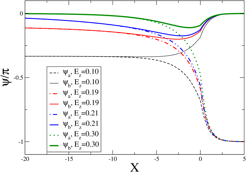
Figure 1: (Color online.) Variation of the canting angles $\psi_{a}$, $\psi_{b}$ with guiding center $X$ (in units of $\ell$), in the presence of an edge near $X=0$. The critical Zeeman energy is $E_{z}^{c}=0.2$.

As the system approaches the transition from the FM side, there is a divergent length scale

$$\xi=\sqrt{\frac{g_{0}+g_{z}-3g_{xy}}{E_{Z}+2g_{xy}}},$$ (3)

so that the edge effectively “expands” into the bulk. In the CAF phase, as noted in the introduction, there is a spontaneously broken symmetry (which can occur in two dimensional systems at $T=0$), which implies the existence of a Goldstone mode Takei2015 . We will explicitly see this mode in our TDHF calculations.

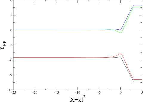
Figure 2: (Color online.) Single-particle energies in the self-consistent HF state at $E_{Z}=0.22$ in the FM phase.

Fig. 2 shows the single-particle spectrum in the HF approximation for $E_{Z}=0.22$ on the FM side of the transition, while Fig. 3 shows it at $E_{Z}=0.18$, in the CAF phase. There is no closing of the gap near the transition. This may seem counterintuitive, especially on the FM side, where the noninteracting model would predict a level crossing between states carrying different spin quantum numbers. However, as noted before, this is due to the spontaneous spin-mixing in HF. Naively, this would indicate that the collective excitations will be gapped at the edge in the FM phase. We will see how TDHF “restores” this symmetry and predicts gapless edge excitations in the next section.

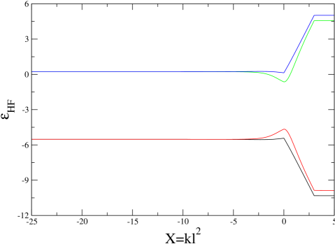
Figure 3: (Color online.) Single-particle energies in the self-consistent HF state at $E_{Z}=0.18$, which is in the canted (CAF) phase. There is no closing of the single-particle gap.

III Time-Dependent Hartree-Fock formalism

The TDHF approximation consists of diagonalizing the Hamiltonian [Eq. (1)] in the Hilbert space of particle-hole excitations. When used in conjunction with the HF approximation, it is “conserving”Kadanoff-Baym , which means that its results, though approximate, respect the symmetries of the underlying Hamiltonian, even if the HF solution breaks it.

Let us briefly go through the TDHF for the bulk.

III.1 Time-Dependent Hartree-Fock approximation in the bulk

The first step is to go to the basis in which the HF Hamiltonian is diagonal. In the bulk this is independent of $k$. Let us call the unitary matrix that carries out this basis change $U$. Explicitly, in terms of $\psi_{a},\ \psi_{b}$, we have

$$U=\left(\begin{array}[]{cccc}\cos{\frac{\psi_{a}}{2}}&-\cos{\frac{\psi_{b}}{2}}&\sin{\frac{\psi_{a}}{2}}&\sin{\frac{\psi_{b}}{2}}\cr-\sin{\frac{\psi_{a}}{2}}&\sin{\frac{\psi_{b}}{2}}&\cos{\frac{\psi_{a}}{2}}&\cos{\frac{\psi_{b}}{2}}\cr\cos{\frac{\psi_{a}}{2}}&\cos{\frac{\psi_{b}}{2}}&\sin{\frac{\psi_{a}}{2}}&-\sin{\frac{\psi_{b}}{2}}\cr\sin{\frac{\psi_{a}}{2}}&\sin{\frac{\psi_{b}}{2}}&-\cos{\frac{\psi_{a}}{2}}&\cos{\frac{\psi_{b}}{2}}\cr\end{array}\right).$$ (4)

We will refer to the four components of each operator $\vec{{\mathbf{c}}}_{k}$ by superscripts, as ${\mathbf{c}}_{k}^{i}$. The subscript $k$ will be reserved for labelling the Landau gauge wavefunctions. The new operators $\vec{{\mathbf{d}}}_{k}$ are related to the old ones $\vec{{\mathbf{c}}}_{k}$ by

$${\mathbf{c}}_{k}^{i}=U_{ij}{\mathbf{d}}_{k}^{j}$$ (5)

In order to re-express the Hamiltonian in terms of ${\mathbf{d}}^{i}_{k}$ it is convenient to define matrices ${\tilde{\mathbf{\tau}}}_{a}$ and ${\tilde{\mathbf{\sigma}}}_{a}$ which are the matrices ${{\mathbf{\tau}}}$ and ${{\mathbf{\sigma}}}$ unitarily transformed into the basis of the $\vec{{\mathbf{d}}}_{k}$. Recalling that the angles $\psi_{a,b}=\psi$ are equal and constant we obtain

$${\tilde{\mathbf{\tau}}}_{x}= U^{\dagger}{{\mathbf{\tau}}}_{x}U=\cos{\psi}{{\mathbf{\tau}}}_{z}{{\mathbf{\sigma}}}_{z}+\sin{\psi}{{\mathbf{\tau}}}_{x},$$ (6)

$${\tilde{\mathbf{\tau}}}_{y}= \cos{\psi}{{\mathbf{\sigma}}}_{y}-\sin{\psi}{{\mathbf{\tau}}}_{y}{{\mathbf{\sigma}}}_{x},$$ (7)

$${\tilde{\mathbf{\tau}}}_{z}= -{{\mathbf{\tau}}}_{z}{{\mathbf{\sigma}}}_{x},$$ (8)

$${\tilde{\mathbf{\sigma}}}_{z}= \cos{\psi}{{\mathbf{\tau}}}_{z}+\sin{\psi}{{\mathbf{\tau}}}_{x}{{\mathbf{\sigma}}}_{z}.$$ (9)

Further defining

$${\tilde{V}}_{ijlm}=\sum\limits_{a=0}^{3}g_{a}\big{(}{\tilde{\mathbf{\tau}}}_{a}\big{)}_{ij}\big{(}{\tilde{\mathbf{\tau}}}_{a}\big{)}_{lm},$$ (10)

we rewrite the Hamiltonian as

$${\mathbf{H}}=\sum\limits_{k}-E_{Z}{\mathbf{d}}^{i\dagger}_{k}{\mathbf{d}}^{j}_{k}\big{(}{\tilde{\mathbf{\sigma}}}_{z}\big{)}_{ij}+\frac{\pi\ell^{2}}{L^{2}}\sum\limits_{kk^{\prime}a{\vec{q}}}e^{-iq_{x}(k-k^{\prime})\ell^{2}-(q\ell)^{2}/2}e^{i[\Phi(k_{1},{\vec{q}})+\Phi(k_{2},-{\vec{q}})]}{\mathbf{d}}^{i\dagger}_{k-q_{y}/2}{\mathbf{d}}^{l\dagger}_{k^{\prime}+q_{y}/2}{\mathbf{d}}^{m}_{k^{\prime}-q_{y}/2}{\mathbf{d}}^{j}_{k+q_{y}/2}{\tilde{V}}_{ijlm}.$$ (11)

The Hartree-Fock Hamiltonian is obtained by reducing the two-body operators to one-body operators by using the expectation values

$$\langle{\mathbf{d}}^{i\,\dagger}_{k_{1}}{\mathbf{d}}^{j}_{k_{2}}\rangle=\delta_{k_{1}k_{2}}\delta_{ij}N_{F}(i),$$ (12)

where $N_{F}(i)=0$ or $1$ is the occupation of the state $i$. We then have

$${\mathbf{H}}_{HF}=\sum\limits_{k}{\mathbf{d}}^{m\,\dagger}_{k}{\mathbf{d}}^{n}_{k}\bigg{(}-E_{Z}{\tilde{\mathbf{\sigma}}}_{z,mn}+\sum\limits_{j}N_{F}(j)({\tilde{V}}_{mnjj}-{\tilde{V}}_{mjjn})\bigg{)}.$$ (13)

In the self-consistent HF state, this one-body hamiltonian is diagonal in the $d$ basis with eigenvalues $\epsilon_{m}$, with $\epsilon_{a}=\epsilon_{b}$ and $\epsilon_{c}=\epsilon_{d}$. Next, we define magnetoexciton operators Kallin1984 with well-defined momentum ${\vec{q}}=(q_{x},q_{y})$ as

$${\mathbf{O}}_{mn}({\vec{q}})=\frac{\sqrt{2\pi\ell^{2}}}{L}\sum\limits_{k}e^{-iq_{x}k\ell^{2}}{\mathbf{d}}^{m\dagger}_{k-q_{y}/2}{\mathbf{d}}^{n}_{k+q_{y}/2}.$$ (14)

One then takes the commutator $[{\mathbf{H}},{\mathbf{O}}^{ij}_{k,q_{y}}]$ which will contain both one-body and two-body terms; the latter are reduced to one-body terms using HF expectation values. After some algebra the final result is

$$[{\mathbf{H}},{\mathbf{O}}_{mn}]|_{HF}=(\epsilon_{m}-\epsilon_{n}){\mathbf{O}}_{mn}({\vec{q}})+e^{-(q\ell)^{2}/2}(N_{F}(n)-N_{F}(m))\sum\limits_{ij}\big{(}{\tilde{V}}_{nmij}-{\tilde{V}}_{imnj}\big{)}{\mathbf{O}}_{ij}({\vec{q}}).$$ (15)

It is clear that the magnetoexciton operators ${\mathbf{O}}_{mn}$ for which $N_{F}(m)=N_{F}(n)$ will propagate freely and will decouple from those with $N_{F}(m)\neq N_{F}(n)$. Thus, we can confine ourselves at each ${\vec{q}}$ to a set of 8 particle-hole operators, which we label by the following assignment to the pair $(m,n)$: $(a,c)\to 1$, $(a,d)\to 2$, $(b,c)\to 3$, $(b,d)\to 4$, $(d,b)\to 5$, $(c,b)\to 6$, $(d,a)\to 7$, and $(c,a)\to 8$. We will identify the first four with bosonic destruction operators ${\mathbf{a}}_{\alpha}$ and the second four with creation operators ${\mathbf{a}}^{\dagger}(-{\vec{q}})$. It can easily be checked that, when HF averages are taken on the right-hand side, the commutators satisfy bosonic relations

$$[{\mathbf{a}}_{\alpha}({\vec{q}}_{1}),{\mathbf{a}}_{\beta}^{\dagger}({\vec{q}}_{2})]|_{HF}= \delta_{\alpha\beta}\delta_{{\vec{q}}_{1}{\vec{q}}_{2}},$$ (16)

$$[{\mathbf{a}}_{\alpha}({\vec{q}}_{1}),{\mathbf{a}}_{\beta}({\vec{q}}_{2})]|_{HF}= 0=[{\mathbf{a}}^{\dagger}_{\alpha}({\vec{q}}_{1}),{\mathbf{a}}^{\dagger}_{\beta}({\vec{q}}_{2})]|_{HF}.$$ (17)

The FM phase is particularly simple since $\psi=0$. In this state the creation and destruction operators do not mix. Defining the notations $\epsilon_{0}=\epsilon_{c}-\epsilon_{a}=2E_{Z}+g_{0}+g_{z}-2{g_{\perp}}$ and $f(q)=e^{-(q\ell)^{2}/2}$ the $4\times 4$ matrix of the TDHF Hamiltonian in the subspace of destruction operators is

$$H^{(+)}_{TDHF}=\left(\begin{array}[]{cccc}-\epsilon_{0}+f(q)(g_{0}+{g_{\perp}})&0&0&-f(q)(g_{z}+{g_{\perp}})\cr 0&-\epsilon_{0}+f(q)(g_{0}-{g_{\perp}})&-f(q)(g_{z}-{g_{\perp}})&0\cr 0&-f(q)(g_{z}-{g_{\perp}})&-\epsilon_{0}+f(q)(g_{0}-{g_{\perp}})&0\cr-f(q)(g_{z}+{g_{\perp}})&0&0&-\epsilon_{0}+f(q)(g_{0}+{g_{\perp}})\cr\end{array}\right).$$ (18)

The TDHF Hamiltonian in the subspace of the creation operators is the same as above, with an overall minus sign. Diagonalization is trivial, leading to the (positive) eigenvalues

$$\omega_{1}(q)= 2E_{Z}+(g_{0}+g_{z})(1-f(q))-2{g_{\perp}}(1+f(q)),$$ (19)

$$\omega_{2}(q)= 2E_{Z}+(g_{0}+g_{z}-2{g_{\perp}})(1-f(q)),$$ (20)

$$\omega_{3}(q)= 2E_{Z}-2{g_{\perp}}+g_{0}(1-f(q))+g_{z}(1+f(q)),$$ (21)

where the last mode is two-fold degenerate. In the limit $q\to 0$ we see that the first mode has a gap of $\omega_{1}(0)=\Delta=2(E_{Z}-E_{Zc})$ where $E_{Zc}=2{g_{\perp}}$. This mode becomes critical at the transition. The second mode has the limit $\omega_{2}(0)=2E_{Z}$ and is the Larmor mode. Note that the Larmor mode is unrenormalized by interactions, as expected from the translational symmetry of the system. This works out correctly even though the energy difference between single-particle eigenstates of the static HF Hamiltonian with opposite spin are interaction-dependent, and is an example of how the TDHF approximation preserves symmetries which may be broken in static HFKadanoff-Baym .

For the canted phase things are a bit more complicated. The single-particle gap is ${\epsilon}_{0}={\epsilon}_{c}-{\epsilon}_{a}=2E_{Z}\cos{\psi}+g_{0}+g_{z}-2{g_{\perp}}\cos{2\psi}$. The creation and destruction subspaces do get mixed by the action of the TDHF Hamiltonian. However, the matrix is block diagonal, with modes $1,4,5,8$ mixing among themselves, while modes $2,3,6,7$ mix among themselves separately. The $4\times 4$ matrix in the $1,4,5,8$ subspace is

$$H_{TDHF}^{(1458)}=\left(\begin{array}[]{cccc}-{\epsilon}_{0}+f(q)(g_{0}+{g_{\perp}})&-f(q)(g_{z}+{g_{\perp}}\cos{2\psi})&2f(q){g_{\perp}}\sin^{2}{\psi}&0\cr-f(q)(g_{z}+{g_{\perp}}\cos{2\psi})&-{\epsilon}_{0}+f(q)(g_{0}+{g_{\perp}})&0&2f(q){g_{\perp}}\sin^{2}{\psi}\cr-2f(q){g_{\perp}}\sin^{2}{\psi}&0&{\epsilon}_{0}-f(q)(g_{0}+{g_{\perp}})&f(q)(g_{z}+{g_{\perp}}\cos{2\psi})\cr 0&-2f(q){g_{\perp}}\sin^{2}{\psi}&f(q)(g_{z}+{g_{\perp}}\cos{2\psi})&{\epsilon}_{0}-f(q)(g_{0}+{g_{\perp}})\cr\end{array}\right).$$ (22)

This can also be easily diagonalized, with the (positive) eigenvalues being

$$\omega_{1}(q)= \sqrt{\big{(}2E_{Z}\cos{\psi}+(g_{0}+g_{z})(1-f(q))-{g_{\perp}}(f(q)+(2+f(q))\cos{2\psi})\big{)}^{2}-4\big{(}{g_{\perp}}f(q)\sin^{2}{\psi}\big{)}^{2}},$$ (23)

$$\omega_{2}(q)= \sqrt{\big{(}2E_{Z}\cos{\psi}+g_{0}(1-f(q))+g_{z}(1+f(q))+{g_{\perp}}(f(q)+(2-f(q))\cos{2\psi})\big{)}^{2}-4\big{(}{g_{\perp}}f(q)\sin^{2}{\psi}\big{)}^{2}}.$$ (24)

Similarly the TDHF matrix in the $2367$ block is

$$H_{TDHF}^{(2367)}=\left(\begin{array}[]{cccc}-{\epsilon}_{0}+f(q)(g_{0}-{g_{\perp}}\cos{2\psi})&-f(q)(g_{z}-{g_{\perp}})&-2f(q){g_{\perp}}\sin^{2}{\psi}&0\cr-f(q)(g_{z}-{g_{\perp}})&-{\epsilon}_{0}+f(q)(g_{0}-{g_{\perp}}\cos{2\psi})&0&-2f(q){g_{\perp}}\sin^{2}{\psi}\cr 2f(q){g_{\perp}}\sin^{2}{\psi}&0&{\epsilon}_{0}-f(q)(g_{0}-{g_{\perp}}\cos{2\psi})&f(q)(g_{z}-{g_{\perp}})\cr 0&2f(q){g_{\perp}}\sin^{2}{\psi}&f(q)(g_{z}-{g_{\perp}})&{\epsilon}_{0}-f(q)(g_{0}-{g_{\perp}}\cos{2\psi})\cr\end{array}\right).$$ (26)

One of the (positive) eigenvalues of this matrix is the same as $\omega_{2}(q)$ above, while the other is

$$\omega_{3}(q)=\sqrt{\big{(}2E_{Z}\cos{\psi}+(g_{0}+g_{z})(1-f(q))-{g_{\perp}}((2-f(q))\cos{2\psi}-f(q))\big{)}^{2}-4\big{(}f(q){g_{\perp}}\sin^{2}{\psi}\big{)}^{2}}.$$ (27)

In the $q\to 0$ limit $\omega_{1}(q)$ is the gapless Goldstone mode, while $\omega_{3}(q)$ is the Larmor mode. The spin-wave velocity of $\omega_{1}(q)$ can be extracted as

$$v_{s}=\ell\sqrt{2{g_{\perp}}\sin^{2}{\psi}\big{(}g_{0}+g_{z}+\frac{E_{Z}^{2}}{2{g_{\perp}}}\big{)}}.$$ (28)

As the system approaches criticality from below, defining $\Delta=E_{Zc}-E_{Z}=2{g_{\perp}}-E_{Z}$ we see that $v_{s}\simeq\sqrt{\Delta}$. Examples of the collective bulk modes for the CAF and FM phases are presented in Figs. 4 and 5.

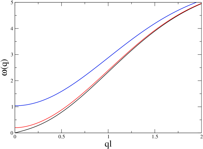
Figure 4: (Color online.) Bulk collective modes at $E_{Z}=0.1$, deep in the CAF phase. Note the linearly dispersing gapless mode which is the Goldstone mode of the broken $U(1)$ symmetry.

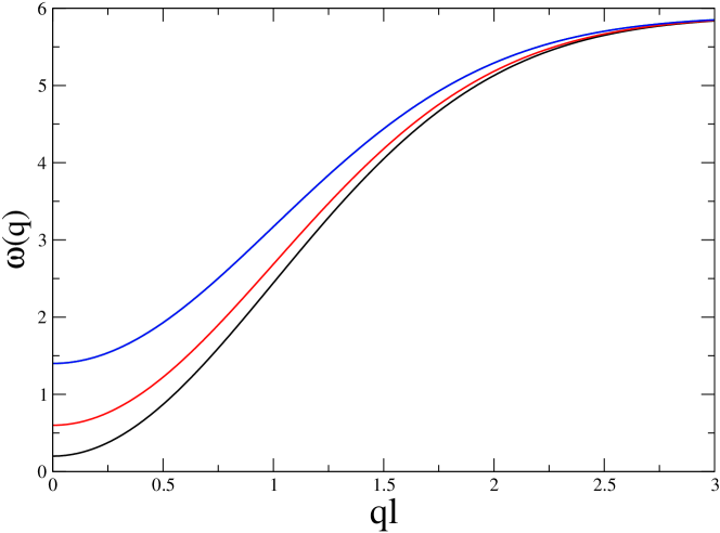
Figure 5: (Color online.) Bulk collective modes at $E_{Z}=0.3$, deep in the FM phase. All modes are robustly gapped.

We next turn to TDHF in the system with an edge, which is considerably more involved.

III.2 Time-Dependent Hartree-Fock approximation with an edge

There are several complications in the system with an edge. Firstly, there is translation invariance only in the $y$ direction, so only $q_{y}$ is a good quantum number for excitations. Secondly, the unitary transformation defined in Eq. (4) will be $k$-dependent. Consequently, the interaction matrix elements in the HF basis will also depend explicitly on $k$,

$${\tilde{V}}_{ijlm}(k_{1},k_{2},q_{y})=\sum\limits_{a=0,x,y,z}g_{a}\big{(}U^{\dagger}(k_{1}-q_{y})\tau_{a}U(k_{1})\big{)}_{ij}\big{(}U^{\dagger}(k_{2}+q_{y})\tau_{a}U(k_{2})\big{)}_{lm}.$$ (29)

The Hamiltonian in this basis is

$${\mathbf{H}}=-\sum\limits_{k}\vec{{\mathbf{d}}}^{\,\dagger}_{k}U^{\dagger}(k)\big{(}E_{Z}\sigma_{z}+U_{e}(k)\tau_{x}\big{)}U(k)\vec{{\mathbf{d}}}_{k}+\frac{\pi\ell^{2}}{L^{2}}\sum\limits_{a,k_{1},k_{2},{\vec{q}}}e^{-\frac{(q\ell)^{2}}{2}}e^{i(\Phi(k_{1},{\vec{q}})+\Phi(k_{2},-{\vec{q}}))}{\tilde{V}}_{ijlm}(k_{1},k_{2},q_{y}){\mathbf{d}}^{i\dagger}_{k_{1}-q_{y}}{\mathbf{d}}^{l\dagger}_{k_{2}+q_{y}}{\mathbf{d}}^{m}_{k_{2}}{\mathbf{d}}^{j}_{k_{1}}.$$ (30)

As in the bulk, the next step is to define the magnetoexciton operators in the $d$ basis. We will keep $L_{y}$ finite, so that the quantum number $q_{y}=\frac{2\pi j_{y}}{L_{y}}$ is discrete, and write

$${\mathbf{O}}^{ij}_{k}(q_{y})={\mathbf{d}}^{i\dagger}_{k-q_{y}}{\mathbf{d}}^{j}_{k}.$$ (31)

One then takes the commutator $[{\mathbf{H}},{\mathbf{O}}^{ij}_{k}(q_{y})]$ which will contain both one-body and two-body terms. We again reduce the two-body terms to one-body terms by using the HF expectation values. In the $d$-basis Eq. (12) remains true independent of $k$; i.e.,

Figure 6: (Color online.) The lowest-lying bulk collective mode as it evolves with $E_{Z}$. It can be seen that the mode becomes gapped at the transition, and the spin-wave velocity vanishes continuously as $E_{Z}\to E_{zc}^{-}$.

$$\langle{\mathbf{d}}^{i\dagger}_{k_{1}}{\mathbf{d}}^{j}_{k_{2}}\rangle=\delta_{k_{1}k_{2}}\delta_{ij}N_{F}(i),$$ (32)

where $N_{F}(i)=0$ or $1$ is the occupation of the state $i$. The analog of Eq. (15) in the system with an edge is

$$[{\mathbf{H}},{\mathbf{O}}^{ij}_{k}(q_{y})]_{HF}= (\epsilon_{i}(k-q_{y})-\epsilon_{j}(k)){\mathbf{O}}^{ij}_{k}(q_{y})+$$

$$\frac{N_{F}(j)-N_{F}(i)}{L_{y}\sqrt{2\pi\ell^{2}}}e^{-\frac{(q_{y}\ell)^{2}}{2}} \sum\limits_{k^{\prime}}e^{-\frac{((k-k^{\prime})\ell)^{2}}{2}}{\mathbf{O}}^{lm}_{k^{\prime}}(q_{y})\big{(}{\tilde{V}}_{jilm}(k-q_{y},k^{\prime},-q_{y})-{\tilde{V}}_{lijm}(k-q_{y},k^{\prime},k-k^{\prime})\big{)}.$$ (33)

Thus, for every value of $q_{y}$ all the ${\mathbf{O}}^{ij}_{k}(q_{y})$ get coupled to each other. This is a matrix diagonalization problem with the dimension of the matrix being proportional to the number of $k$ values kept. As one approaches the transition, due to the diverging length scale more $k$ values have to be retained.

As in the bulk, one needs to consider only the operators which connect filled with empty HF levels. Let us order the index $i=1,2,3,4$ in order of increasing HF energy. Then $N_{F}(1)=N_{F}(2)=1$ and $N_{F}(3)=N_{F}(4)=0$. It is convenient to divide the operators into two groups: positive energy operators ${\mathbf{O}}^{ij,(+)}_{k}(q_{y})$ have $i<j$ while negative energy operators ${\mathbf{O}}^{ij,(-)}_{k}(q_{y})$ have $i>j$. They are related by

$${\mathbf{O}}^{ij,(-)}_{k}(q_{y})=\big{(}{\mathbf{O}}^{ji,(+)}_{k+q_{y}}(-q_{y})\big{)}^{\dagger}.$$ (34)

To simplify the notation let us introduce a composite label for the positive energy operators $\alpha={i,j,+,k}$ and the notation

$${\mathbf{a}}_{\alpha}(q_{y})={\mathbf{O}}^{ij,(+)}_{k}(q_{y}).$$ (35)

These operators share many features of canonical boson operators. In particular, they satisfy canonical commutation relations upon taking a HF average,

$$[{\mathbf{a}}_{\alpha}(q_{y}),{\mathbf{a}}^{\dagger}_{\beta}(q_{y}^{\prime})]|_{HF}=\delta_{\alpha\beta}\delta_{q_{y}q_{y}^{\prime}}.$$ (36)

The TDHF equations can then be written as

$$[{\mathbf{H}},{\mathbf{a}}_{\alpha}(q_{y})]=\sum\limits_{\beta}\big{(}A_{\alpha\beta}(q_{y}){\mathbf{a}}_{\beta}(q_{y})+B_{\alpha\beta}(q_{y}){\mathbf{a}}^{\dagger}_{\beta}(-q_{y})\big{)}$$ (37)

and its adjoint. Note that these equations can be thought of as arising from the Bogoliubov Hamiltonian

$${\mathbf{H}}_{B} =-\sum\limits_{\alpha\beta}\big{(}A_{\alpha\beta}(q_{y}){\mathbf{a}}^{\dagger}_{\alpha}(q_{y}){\mathbf{a}}_{\beta}(q_{y})+h.c.$$ (38)

$$+B_{\alpha\beta}(q_{y}){\mathbf{a}}^{\dagger}_{\alpha}(q_{y}){\mathbf{a}}^{\dagger}_{\beta}(-q_{y})+h.c.\big{)}.$$

Diagonalizing this Hamiltonian corresponds to finding eigenoperators ${\mathbf{b}}_{\mu}(q_{y})$, ${\mathbf{b}}^{\dagger}_{\mu}(-q_{y})$ such that

$$[{\mathbf{H}}_{B},{\mathbf{b}}_{\mu}(q_{y})] =-E_{\mu}(q_{y}){\mathbf{b}}_{\mu}(q_{y}),$$ (39)

$$[{\mathbf{H}}_{B},{\mathbf{b}}^{\dagger}_{\mu}(q_{y})] =E_{\mu}(q_{y}){\mathbf{b}}^{\dagger}_{\mu}(q_{y}).$$ (40)

This makes it evident that the eigenvalues of $H_{B}$ come in $\pm$ pairs. The eigenoperators can be expressed in the original $\alpha$ basis as

$${\mathbf{b}}_{\mu}(q_{y})= \sum\limits_{\alpha}\big{(}\psi^{(+)}_{<,\mu\alpha}(q_{y}){\mathbf{a}}_{\alpha}(q_{y})+\psi^{(-)}_{<,\mu\alpha}(q_{y}){\mathbf{a}}^{\dagger}_{\alpha}(-q_{y})\big{)},$$ (42)

$${\mathbf{b}}^{\dagger}_{\mu}(-q_{y})= \sum\limits_{\alpha}\big{(}\psi^{(+)}_{>,\mu\alpha}(q_{y}){\mathbf{a}}_{\alpha}(q_{y})+\psi^{(-)}_{>,\mu\alpha}(q_{y}){\mathbf{a}}^{\dagger}_{\alpha}(-q_{y})\big{)}.$$ (43)

It is important to note that the orthonormalization of the “wavefunctions” $\psi^{(\pm)}_{\mu\alpha}$ is determined by the commutation relation of the operators $b_{\mu},\ b^{\dagger}_{\mu}$

$$[{\mathbf{b}}_{\mu}(q_{y}),{\mathbf{b}}^{\dagger}_{\nu}(q_{y}^{\prime})] =\delta_{\mu\nu}\delta_{q_{y}q_{y}^{\prime}},$$

$$[{\mathbf{b}}_{\mu}(q_{y}),{\mathbf{b}}_{\nu}(q_{y}^{\prime})] =[{\mathbf{b}}^{\dagger}_{\mu}(q_{y}),{\mathbf{b}}^{\dagger}_{\nu}(q_{y}^{\prime})]=0,$$ (44)

which imply

$$\sum\limits_{\alpha}\psi^{(+)}_{<,\mu\alpha}(q_{y})\psi^{(+)*}_{<,\nu\alpha}(q_{y}^{\prime})-\psi^{(-)}_{<,\mu\alpha}(q_{y})\psi^{(-)*}_{<,\nu\alpha}(q_{y}^{\prime})=\delta_{\mu\nu}\delta_{q_{y}q_{y}^{\prime}},$$ (45)

$$\sum\limits_{\alpha}\psi^{(-)*}_{>,\mu\alpha}(q_{y})\psi^{(-)}_{>,\nu\alpha}(q_{y}^{\prime})-\psi^{(+)*}_{>,\mu\alpha}(q_{y})\psi^{(+)}_{>,\nu\alpha}(q_{y}^{\prime})=\delta_{\mu\nu}\delta_{q_{y}q_{y}^{\prime}},$$ (46)

$$\sum\limits_{\alpha}\psi^{(+)}_{<,\mu\alpha}(q_{y})\psi^{(+)*}_{>,\nu\alpha}(q_{y}^{\prime})-\psi^{(-)}_{<,\mu\alpha}(q_{y})\psi^{(-)*}_{>,\nu\alpha}(q_{y}^{\prime})=0.$$ (47)

This provides us with a complete set of one-body operators in terms of which any operator can be expanded, and can be exploited to find linear response functions.

Consider a one-body operator ${\mathbf{Q}}(q_{y})$. In the original basis we can expand it as

$${\mathbf{Q}}(q_{y})=\sum\limits_{\alpha}Q^{(+)}_{\alpha}(q_{y}){\mathbf{a}}_{\alpha}(q_{y})+Q^{(-)}_{\alpha}(q_{y}){\mathbf{a}}^{\dagger}_{\alpha}(q_{y}).$$ (48)

Employing Eq. (43), we can also expand $Q$ in the eigenbasis of the TDHF Hamiltonian as

$${\mathbf{Q}}(q_{y})=\sum\limits_{\mu}R^{(+)}_{\mu}(q_{y}){\mathbf{b}}_{\mu}(q_{y})+R^{(-)}_{\mu}(q_{y}){\mathbf{b}}^{\dagger}_{\mu}(q_{y}).$$ (49)

To find the coefficients $R$ we simply take the commutator of $Q$ with ${\mathbf{b}}_{\mu},\ {\mathbf{b}}^{\dagger}_{\mu}$, or alternatively use the orthonormalization conditions, to obtain

$$R^{(+)}_{\mu}= \sum\limits_{\alpha}Q^{(+)}_{\alpha}\psi^{(+)*}_{<\mu\alpha}-Q^{(-)}_{\alpha}\psi^{(-)*}_{<\mu\alpha},$$ (50)

$$R^{(-)}_{\mu}=- \sum\limits_{\alpha}Q^{(+)}_{\alpha}\psi^{(+)*}_{>\mu\alpha}-Q^{(-)}_{\alpha}\psi^{(-)*}_{>\mu\alpha},$$ (51)

where we have suppressed the argument $q_{y}$ for compactness. Now the retarded $QQ$ response function can be written in the frequency domain as

$$\chi_{QQ}(q_{y},\omega)=\sum\limits_{\mu}\bigg{(}\frac{|R^{(+)}_{\mu}(q_{y})|^{2}}{\omega+i\eta+E_{\mu}(q_{y})}-\frac{|R^{(-)}_{\mu}(q_{y})|^{2}}{\omega+i\eta-E_{\mu}(q_{y})}\bigg{)}.$$ (52)

Finally, the spectral density is defined by

$$S_{QQ}(q_{y},\omega)=-\pi Im\big{(}\chi_{QQ}(q_{y},\omega)\big{)}.$$ (53)

Since we are trying to find experimental signatures of the two phases, we will focus on one-body operators that naturally couple to external probes, which include the charge density and spin densities. When computing response functions, we will assume that we are coupling the relevant operator in a strip of width $\ell$. The perturbation coupling to the density operator with $y$-momentum $q_{y}$, for example, will have the form

$${\mathbf{Q}}_{\rho}(q_{y}) = \sum\limits_{k}e^{-(k-k_{0})^{2}\ell^{2}/2}\vec{{\mathbf{c}}}^{\dagger}_{k-q_{y}}\vec{{\mathbf{c}}}_{k}$$

$$= \sum\limits_{k}e^{-(k-k_{0})^{2}\ell^{2}/2}\vec{{\mathbf{d}}}^{\,\dagger}_{k-q_{y}}U^{\dagger}(k-q_{y})U(k)\vec{{\mathbf{d}}}_{k}$$

When $k_{0}$ is near the edge, this will couple primarily to edge modes, whereas if $k_{0}$ is deep in the bulk, it couples solely to bulk modes. Deep in the bulk, since the angles $\psi_{a,b}$ are constant, $U^{\dagger}(k-q_{y})U(k)=1$, so ${\mathbf{Q}}_{\rho}$ is diagonal in the $\vec{{\mathbf{d}}}$ basis. Thus, there is no response to a density perturbation in the bulk.

Similar expressions for the spin-density operators are

$${\mathbf{S}}^{a}=\sum\limits_{k}e^{-(k-k_{0})^{2}\ell^{2}/2}\vec{{\mathbf{d}}}^{\,\dagger}_{k-q_{y}}U^{\dagger}(k-q_{y})\sigma_{a}U(k)\vec{{\mathbf{d}}}_{k}.$$ (55)

Exactly as above, in the FM phase, there is no response to ${\mathbf{S}}^{z}$.

We now proceed to the results.

IV Results of the TDHF approximation

We will focus on correlators of interest, specifically the density-density, $S_{z}S_{z}$, $S_{x}S_{x}$, and $S_{y}S_{y}$ correlators. In each case we will plot the spectral density of the correlator, the peaks of which will give us an indication of the excitations that this correlator couples to, both for the bulk and the edge. The latter will reveal the distinct character of the edge excitations.

In carrying out TDHF for the bulk, one can use translation invariance to assume that both $q_{x}$ and $q_{y}$ are good quantum numbers. This reduces the problem to the diagonalization of an $8\times 8$ matrix. For the edge, we use a “bulk” of length $80\ell$ and an edge of length $4\ell$. We choose $L_{y}=20\pi\ell$ so that the separation between successive values of $k\ell^{2}$ is $0.1\ell$. This set of parameters leads to the a TDHF matrix of dimension roughly $7000\times 7000$. The finite size of the bulk means that we cannot approach the phase transition too closely, because when the length scale $\xi$ of Eq. (3) becomes comparable to the system size it is impossible to separate the edge and the bulk.

Another consequence of the finite system size is that the spectrum is discrete. So in computing the spectral density of Eq. (53) we replace the Dirac $\delta$-functions by Lorentzians of width $\eta=0.05$, which produces fairly smooth spectral densities.

Below we use the parameters of the model given in Section II. In particular, the critical point is at $E_{Z}=0.2$.

IV.1 Bulk Collective Modes

We begin by presenting the evolution of the bulk collective modes as $E_{Z}$ increases. Fig. 4 shows them deep in the CAF phase at $E_{Z}=0.1$. As expected from the spontaneously broken symmetry, the lowest bulk mode (black line) is a gapless linearly dispersing Goldstone mode. The next mode (blue) is the Larmor mode, and goes to the limit $\omega(q=0)=2E_{Z}$. The highest energy mode is two-fold degenerate.

In Fig. 5, we present the bulk modes at $E_{Z}=0.3$, deep in the FM phase. There is no spontaneously broken symmetry, so there is no gapless bulk mode in this phase. The gap for the lowest mode is $\Delta=2(E_{Z}-E_{Zc})$. Fig. 6 shows the evolution of the lowest-lying collective bulk mode as a function of $E_{Z}$. It is evident that the spin-wave velocity in the CAF phase vanishes continuously as the transition is approached. At $E_{Z}=E_{Zc}$ the lowest-lying mode becomes quadratically dispersing, and for $E_{Z}>E_{Zc}$ it “lifts off” and becomes gapped.

Now we are ready to look at the correlators in the bulk. Within the $\nu=0$ Landau level, in a translationally invariant HF state, the charge density operator does not couple to leading order to the collective excitations. We will thus restrict ourselves to the spin correlators in the bulk.

IV.2 Bulk Spin Correlators

We begin with the $S_{z}S_{z}$ correlator for the CAF phase. In Fig. 7 we show this correlator in the bulk at $E_{Z}=0.1$, deep in the CAF phase.

Figure 7: (Color online.) The spectral density of the $S_{z}S_{z}$ correlator at $E_{Z}=0.1$, deep in the CAF phase. The coupling to the gapless Goldstone mode can be seen.

Due to the condensation of $S_{x}$, the operator $S_{z}$ is subject to quantum fluctuations, and couples strongly to the Goldstone mode. In principle this is an unambiguous way of detecting the CAF phase. The $S_{x}S_{x}$ and $S_{y}S_{y}$ correlators, on the other hand, couple only to the Larmor mode, and their spectral densities are correspondingly gapped, as seen in Fig. 8.

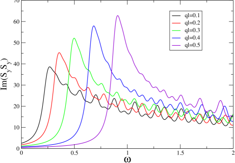
Figure 8: (Color online.) The spectral density of the $S_{y}S_{y}$ correlator at $E_{Z}=0.1$, deep in the CAF phase. The coupling to the gapped Larmor mode can be seen.

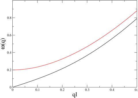
Figure 9: (Color online.) An expanded view of the lowest two modes at $E_{Z}=0.1$.

To help with the comparison of the peak positions of the spectral densities, we provide an expanded view of the Goldstone mode and the Larmor mode for $E_{Z}=0.1$ in Fig. 9. At $q_{y}\ell=0.1$, for example, the $S_{z}S_{z}$ spectral function peaks at $\omega\approx 0.1$, which is the Goldstone mode energy, while the $S_{y}S_{y}$ spectral density peaks at $\omega\approx 0.25$, which is the Larmor mode energy. As $q_{y}$ increases, the difference in peak position persists, but becomes smaller as the modes become similar in energy.

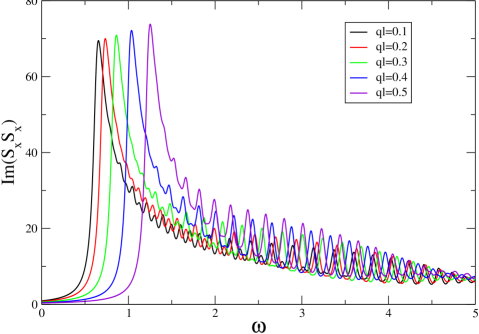
Figure 10: (Color online.) The spectral density of the $S_{x}S_{x}$ correlator at $E_{Z}=0.3$, deep in the FM phase.

Now we go deep into the FM phase. Here $S_{z}$ is a good quantum number, so there are no fluctuations and the $S_{z}S_{z}$ correlator is trivial. The $S_{x}S_{x}$ and $S_{y}S_{y}$ correlators once again follow the Larmor mode, as shown in Fig. 10. The gap is larger ($2E_{Z}=0.6$) and therefore easier to see than at $E_{Z}=0.1$.

IV.3 Edge Modes and Correlators

Let us start with the dispersion of collective particle-hole modes in a system with an edge. Fig. 11 shows the first few modes at $E_{Z}=0.1$, in the CAF phase. Since only $q_{y}$ is a good quantum number, all the values of $q_{x}$, which were good quantum numbers in the bulk, are now potentially mixed. The bottom of the quasi-continuum is the bulk gapless mode, shown in the bold black line.

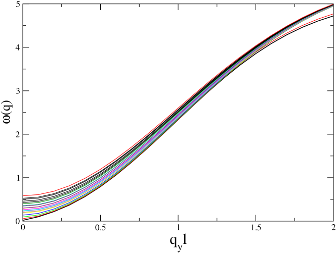
Figure 11: (Color online.) The energy dispersion of collective particle-hole excitations vs $q\ell$ for a system with an edge at $E_{Z}=0.1$ in the CAF phase. The figure looks dense because only $q_{y}$ is a good quantum number, so all the possible values of $q_{x}$ may get mixed.

Things become more interesting when we go to the FM phase. Recall that, as seen in Fig. 5, the bulk was gapped in this phase. The first few modes in the system with an edge at $E_{Z}=0.22$ are shown in Fig. 12. As can be seen there is now a gapless mode (thick black line) which was not present in the bulk system. This becomes even clearer when one goes deeper into the FM phase, as shown in Fig. 13. Thus the TDHFA supports the expectation that the FM state, despite having a gapped HF spectrum, supports gapless edge modes Kharitonov_edge ; Murthy2014 . This is another example of the way TDHF restores the symmetry broken by the HF approximation. The naive view, that the gapless mode is the Goldstone mode of the symmetry broken in HF, is incorrect in this case: In a 1D system, a continuous symmetry cannot be broken even at $T=0$, and the symmetry-breaking seen in HF is an artefact.

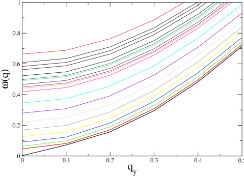
Figure 12: (Color online.) The energy dispersion of collective particle-hole excitations vs $q\ell$ for a system with an edge at $E_{Z}=0.22$, close to the transition in the FM phase. Note the gapless mode (thick black line) which was absent in the bulk spectrum of Fig. 5.

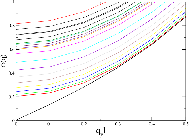
Figure 13: (Color online.) The energy dispersion of collective particle-hole excitations vs $q\ell$ for a system with an edge at $E_{Z}=0.3$, deep in the FM phase. Note the gapless mode (thick black line) which was absent in the bulk spectrum of Fig. 5.

There is another important aspect to the physics of the gapless edge mode: it must be able to carry charge. To ascertain that this is indeed true we look at the spectral density of the charge-charge correlator in the system with an edge. Fig. 14 shows the spectral density of the charge correlator at $E_{Z}=0.3$, deep in the FM phase. The peaks dispersing linearly as a function of $q\ell$ show that the gapless edge mode indeed carries charge. Fig. 15 shows that this persists close to the transition. However, in this situation, the gapless edge mode admixes with low-energy gapped bulk modes, leading to some broadening. (This may have important consequences for transport at finite temperature, a subject we will address in a future publication.)

We also note that in addition to the gapless edge mode, the charge density correlator also couples to a high-energy mode (with an energy around $\omega\approx 4$ in our units). This could be a gapped charge-carrying mode bound to the edge, and seems to stiffen as one approaches the critical point.

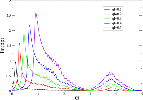
Figure 14: (Color online.) The spectral density of the charge density-density correlator as a function of $\omega$ for different values of $q_{y}\ell$ at $E_{Z}=0.3$ deep in the FM phase. Note the peaks at low $\omega$ which correspond to the gapless edge modes in Fig. 13.

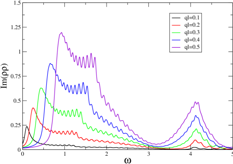
Figure 15: (Color online.) The spectral density of the charge density-density correlator as a function of $\omega$ for different values of $q_{y}\ell$ at $E_{Z}=0.22$, close to the transition but in the FM phase. Note the peaks at low $\omega$ which correspond to the gapless edge modes in Fig. 12.

In Fig. 16 we show the spectral density of the charge correlator at $E_{Z}=0.1$, deep in the CAF phase. The gapped nature of the excitations coupling to charge is evident. As one approaches very close to the transition, the finite size effects mentioned at the beginning of the section come into play. The quantum phase transition, which would have been sharp in a thermodynamically large system, becomes instead a crossover. This is seen in the spectral density of charge correlator at $E_{Z}=0.18$, shown in Fig. 17. As at $E_{Z}=0.22$ [Fig. 15], one can see that both the gapless (bulk) mode and a gapped mode contribute. We have checked that the contribution of the gapless mode decreases as the system size is increased, whereas the contribution of the gapped mode does not change. The contribution of the gapped charge-carrying mode noted in the F phase persists in the CAF phase as well.

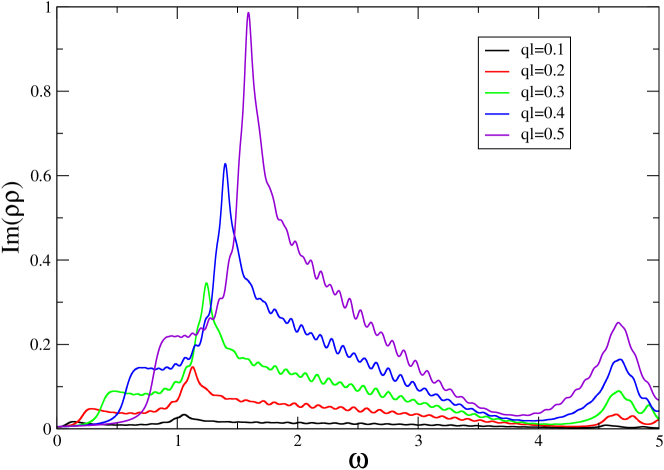
Figure 16: (Color online.) The spectral density of the charge density-density correlator as a function of $\omega$ for different values of $q_{y}\ell$ at $E_{Z}=0.10$, deep in the CAF phase. Note that the peaks in the spectral density are gapped, indicating that the charge does not couple to the gapless Goldstone mode.

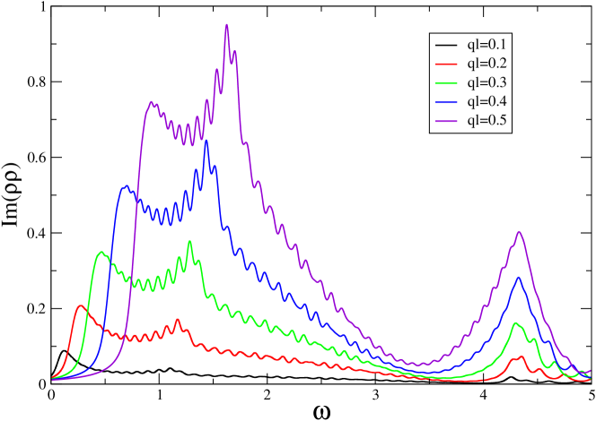
Figure 17: (Color online.) The spectral density of the charge density-density correlator as a function of $\omega$ for different values of $q_{y}\ell$ at $E_{Z}=0.18$, close to the transition in the CAF phase. There are now contributions from both gapless and gapped modes, presumably due to finite-size effects.

To complete the picture, let us examine the spin correlators.

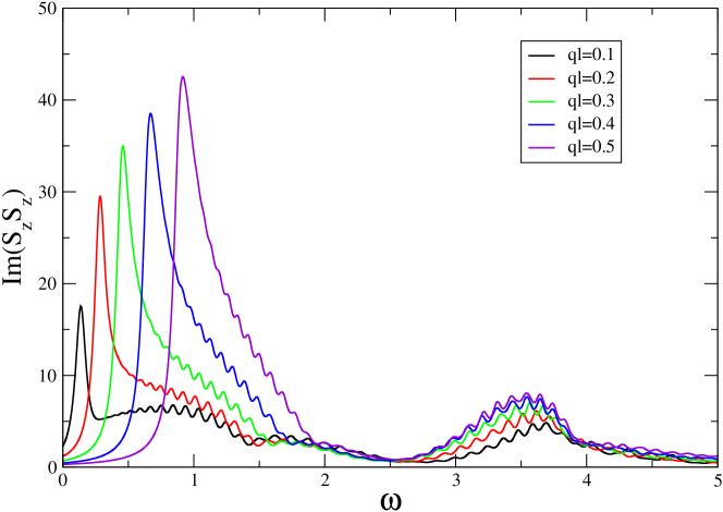
Figure 18: (Color online.) The spectral density of the $S_{z}S_{z}$ correlator as a function of $\omega$ for different values of $q_{y}\ell$ at $E_{Z}=0.30$, deep in the FM phase. In contrast to the bulk correlator, this spectral density couples strongly to the gapless edge mode.

This time we will start in the FM phase. As noted in the previous subsection, the bulk $S_{z}S_{z}$ correlator is trivial in the FM phase, because the bulk is fully polarized. In Fig. 18 we see that this is not the case when an edge is present. The spectral density of this correlator couples to the gapless mode as well. This can be understood from an effective field theory as follows: The one-dimensional field theory describing the edge deep in the FM phase is a helical Luttinger liquid Fertig2006 ; SFP , in which the right-movers have spin up (say) and left-movers have spin down. In such a system the charge current is proportional to the $S_{z}$-density. Thus, it is natural that the $S_{z}S_{z}$ correlator couples to these gapless excitations. Unfortunately, this by itself cannot be used as a signature of the phase transition because the qualitative behavior is the same in the CAF phase, as shown in Fig. 19. Here the gapless mode the correlator couples to is the bulk Goldstone mode.

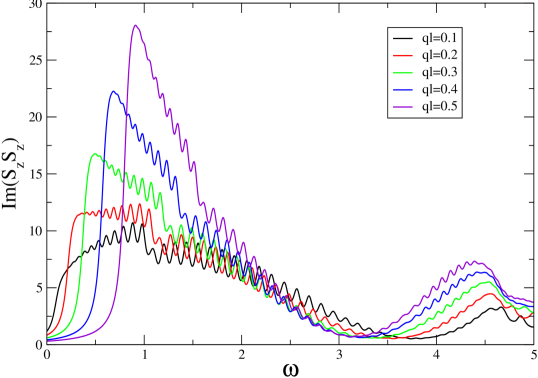
Figure 19: (Color online.) The spectral density of the $S_{z}S_{z}$ correlator as a function of $\omega$ for different values of $q_{y}\ell$ at $E_{Z}=0.10$, deep in the CAF phase. The peaks now indicate a coupling to the Goldstone mode.

IV.4 Space and Time-Dependent Response at the Edge

The linearly dispersing mode at the edge can be seen in a much more physical way. Imagine that we make a localized (in both space and time) perturbation at a particular position at the edge. If there is a linearly dispersing mode that couples to the physical perturbation in question, the effects can propagate arbitrarily far. To be specific, let us consider a perturbation (induced by, e.g., a field pulse) of the form

$${\mathbf{H}}\to{\mathbf{H}}+Ce^{-\frac{y^{2}}{2\lambda^{2}}-\frac{t^{2}}{2\tau^{2}}}{\mathbf{Q}}(y,t).$$ (56)

By expanding ${\mathbf{Q}}$ in terms of the eigenoperators of the TDHF Hamiltonian (Eq. 49), after a few straightforward manipulations we obtain

$$\langle{\mathbf{Q}}(y,t)\rangle\propto\int\limits_{0}^{\infty}\frac{d\omega}{\pi}\sum\limits_{{\vec{q}}}e^{-(q\lambda)^{2}/2-t^{2}/2\tau^{2}}\sin(qy-\omega t)S_{QQ}(q,\omega).$$ (57)

Fig. 20 illustrates the response to a density perturbation at the edge (localized at $y=t=0$) deep in the FM phase measured at different values of $y$ as a function of time. The propagating mode manifests itself as a peak that shifts to later times as one moves further away.

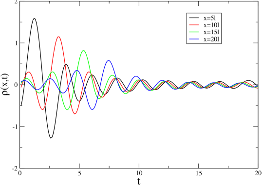
Figure 20: (Color online.) The $t$-dependent response at different locations to a localized density perturbation along the edge at $E_{Z}=0.3$. The linear edge mode produces a travelling pulse.

The same is seen when the perturbation is in $S_{z}$ instead of $\rho$ (see Fig. 21), which is consistent with the interpretation of the edge as a helical Luttinger liquid.

When we go deep into the CAF phase, we do not expect a propagating edge mode that couples to density. As seen in Fig. 22 the response as a function of time is only weakly dependent on the position. However, if the perturbation is in $S_{z}$, Fig. 23 shows that there is a propagating mode, which we can assume to be the bulk Goldstone mode.

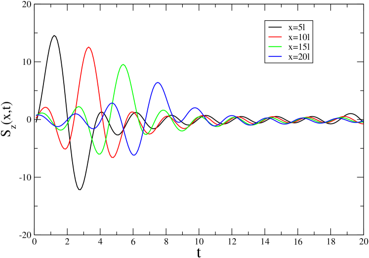
Figure 21: (Color online.) The $t$-dependent response at different locations to a localized $S_{z}$ perturbation along the edge at $E_{Z}=0.3$. The linear edge mode produces a travelling pulse.

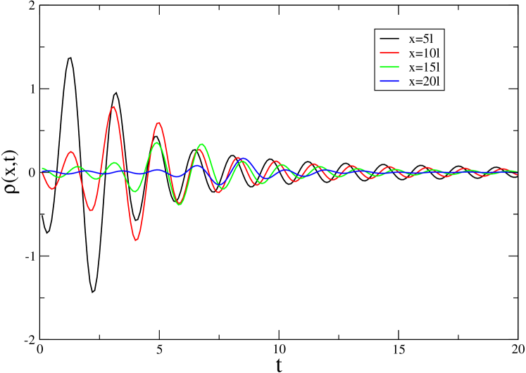
Figure 22: (Color online.) The $t$-dependent response at different locations to a localized density perturbation along the edge at $E_{Z}=0.1$. There is no travelling pulse showing the absence of an edge mode coupling to charge.

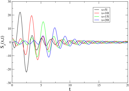
Figure 23: (Color online.) The $t$-dependent response at different locations to a localized $S_{z}$ perturbation along the edge at $E_{Z}=0.1$. The coupling to the bulk Goldstone mode produces a travelling pulse.

V Summary, Conclusions and Open Questions

In this paper we investigate the nature of collective particle-hole excitations in $\nu=0$ single-layer graphene. This system has been shown experimentallyYoung2013 to undergo a quantum phase transition as a function of Zeeman coupling $E_{Z}$. For $E_{Z}<E_{Zc}$ the state is an insulator, while for $E_{Z}>E_{Zc}$ there are conducting edge modes robust to disorder. A simple model proposed by KharitonovKharitonov_bulk ; Kharitonov_edge displays precisely such a phase transition, explaining it as a transition from a canted antiferromagnet (CAF) phase in which charge modes are fully gapped to a fully polarized ferromagnetic (FM) phase which has gapless edge modes.

In previous work Murthy2014 we carried out a static Hartree-Fock analysis on Kharitonov’s model in a system with an edge, showing that the occupied manifold could be characterized by two angles $\psi_{a,b}$ which characterized entanglement between the spin and valley sectors. These angles became equal deep in the bulk, but differed near the edge. We proposed an ansatz for charge excitations bound to the edge, and showed that while in the CAF phase they are gapped, they become gapless in the FM phase.

In this paper these ideas are substantiated in the time-dependent Hartree-Fock (TDHF) approximation and physically measurable correlation functions are computed, both for the bulk and the edge.

In the bulk FM phase, the density and $S_{z}$ correlators are fully gapped. As one goes through the transition into the CAF phase there is a divergent length scale, associated with the vanishing of the gap of the critical mode. At the critical point it becomes quadratically dispersing.

Unfortunately, there seems to be no simple way to probe the critical mode in the bulk FM phase. It does not couple to any of the natural physical observables, such as components of spin or the charge density. It may, in principle, be possible to infer its existence by indirect means. For example, when the mode gets low enough, it should hybridize with sound waves, and may show up in acoustic attenuation. If some analog of inelastic light scattering were possible in single-layer graphene, it should be visible there as well.

In the bulk CAF phase the symmetry breaking represented by the angles $\psi_{a,b}\neq 0$ leads to a neutral Goldstone mode, which can be seen in the $S_{z}S_{z}$ correlator. The $S_{x}S_{x}$ and $S_{y}S_{y}$ correlators have spectral densities coupling to the Larmor mode, which is gapped in both phases and through the transition. The signature of the bulk CAF phase is the gaplessness of the spectral density of the $S_{z}S_{z}$ correlator. This spectral density becomes gapped at the phase transition. In principle, the gapless $S_{z}S_{z}$ correlator could be used to distinguish the CAF phase from other proposals for the $\nu=0$ QH state, such as singlet KekuleKekule or charge density wave phases.

Coming now to the edge, we clearly see a gapless, linearly dispersing, non-chiral charge-carrying edge mode throughout the FM phase. One can interpret this as the helical mode of a strongly interacting Luttinger liquid at the edge, an interpretation we will explore in detail in future work. This mode shows up in the spectral densities of both the $\rho\rho$ and the $S_{z}S_{z}$ correlators. When one goes through the transition into the CAF phase, the $\rho\rho$ correlator should become gapped. We do see the gapped nature deep in the CAF phase, but close to the transition, the finite size of our system leads to some “contamination” from the gapless Goldstone mode of the CAF bulk.

Many open questions remain. While the HF and TDHF approximations are adequate far from the transition, we expect interaction corrections beyond TDHF to play a role close to the transition. The bulk transition is in the same universality class as the Bose-HubbardBose-Hubbard superfluid-insulator transition away from the tip of the Mott lobesMa-Halperin-Lee . It has dynamical critical exponent $z=2$, and at $T=0$ the interactions will be marginally (but dangerously) irrelevant. Even more important is the effect of these critical fluctuations on the charge-carrying modes at the edge, and thus on the transport. Last, but not least, we have assumed the system to be clean. Disorder could have a profound and nonperturbative effectBose-Hubbard on the region near the phase transition of the clean system. We hope to address these and other questions in the near future.

Useful discussions with A. Young, P. Jarillo-Herrero, R. Shankar, and E. Berg are gratefully acknowledged. The authors thank the Aspen Center for Physics (NSF Grant No. 1066293) for its hospitality, and for support by the Simons Foundation (ES). This work was supported by the US-Israel Binational Science Foundation (BSF) grant 2012120 (ES, GM, HAF), the Israel Science Foundation (ISF) grant 231/14 (ES), and NSF-DMR 1306897 (GM), and by NSF-DMR 1506460.

References

- (1) Y. Zhang, Z. Jiang, J. P. Small, M. S. Purewal, Y.-W. Tan, M. Fazlollahi, J. D. Chudow, J. A. Jaszczak, H. L. Stormer, and P. Kim, Phys. Rev. Lett. bf 96, 236806 (2006).
- (2) J. Alicea and M.P.A. Fisher, Phys. Rev. B. 74, 075422 (2006).
- (3) M.O. Goerbig, R. Moessner, and B. Doucot, Phys. Rev. B 74, 161407 (2006).
- (4) V.P. Gusynin, V.A. Miransky, S.G. Sharapov, and I. Shovkovy, Phys. Rev. B 74, 195429 (2006).
- (5) K. Nomura and A.H. MacDonald, :hys. Rev. Lett. 96, 256602 (2006).
- (6) Z. Jiang, Y. Zhang, H. L. Stormer, and P. Kim, Phys. Rev. Lett. 99, 106802 (2007).
- (7) I.F. Herbut, Phys. Rev. B. 75, 165411 (2007)
- (8) J.N. Fuchs and P. Lederer, Phys. Rev. Lett. 98, 016803 (2007).
- (9) D. A. Abanin, K. S. Novoselov, U. Zeitler, P. A. Lee, A. K. Geim and L. S. Levitov, Phys. Rev. Lett. 98, 196806 (2007).
- (10) J. G. Checkelsky, L. Li and N. P. Ong, Phys. Rev. Lett. 100, 206801 (2008); J. G. Checkelsky, L. Li and N. P. Ong, Phys. Rev. B 79, 115434 (2009).
- (11) Xu Du, I. Skachko, F. Duerr, A. Luican, and E. Y. Andrei, Nature 462, 192 (2009).
- (12) M.O. Goerbig, Rev. Mod. Phys. 83, 1193 (2011).
- (13) Andrea F. Young, Cory R. Dean, Lei Wang, Hechen Ren, Paul Cadden-Zimansky, Kenji Watanabe, Takashi Taniguchi, James Hone, Kenneth L. Shepard, Philip Kim, Nat. Phys. 8, 550 (2012).
- (14) G. L. Yu, R. Jalil, Branson Belle, Alexander S. Mayorov, Peter Blake, Frederick Schedin, Sergey V. Morozov, Leonid A. Ponomarenko, F. Chiappini, S. Wiedmann, Uli Zeitler, Mikhail I. Katsnelson, A. K. Geim, Kostya S. Novoselov, Daniel C. Elias, PNAS 110, 3282 (2013).
- (15) I.F. Herbut, Phys. Rev. B 76, 085432 (2007).
- (16) J. Jung and A.H. MacDonald, Phys. Rev. B 80, 235417 (2009).
- (17) R. Nandkishore and L. S. Levitov, Phys. Scr. T146, 014011 (2009); R. Nandkishore and L. S. Levitov, arXiv:1002.1966.
- (18) M. Kharitonov, Phys. Rev. B 85, 155439 (2012).
- (19) Bitan Roy, M.P. Kennett, and S. Das Sarma, arXiv:1406.5184.
- (20) J.L. Lado and J. Fernandez-Rossier, arXiv:1406.6016.
- (21) Y. Zhang, Z. Jiang, J. P. Small, M. S. Purewal, Y.-W. Tan, M. Fazlollahi, J. D. Chudow, J. A. Jaszczak, H. L. Stormer and P. Kim, Phys. Rev. Lett. 96, 136806 (2006); Y. Zhao, P. Cadden-Zimansky, F. Ghahari and P. Kim, Phys. Rev. Lett. 108, 106804 (2012).
- (22) A. F. Young, J. D. Sanchez-Yamagishi, B. Hunt, S. H. Choi, K. Watanabe, T. Taniguchi, R. C. Ashoori, P. Jarillo-Herrero, Nature 505, 528 (2014).
- (23) A similar behavior has been detected in bilayer graphene: P. Maher, C. R. Dean, A. F. Young, T. Taniguchi, K. Watanabe, K. L. Shepard, J. Hone and P. Kim, Nature Physics 9, 154 (2013).
- (24) An analogous transition has been proposed for quantum Hall bilayer systems at filling factor . See, for example, S. Das Sarma, Subir Sachdev, and Lian Zheng, Phys. Rev. Lett. 79, 917 (1997); L. Brey, Phys. Rev. Lett. 81, 4692 (1998); J. Schliemann and A.H. MacDonald, Phys. Rev. Lett. 84, 4437 (2000).
- (25) V. P. Gusynin, V. A. Miransky, S. G. Sharapov, and I. A. Shovkovy, Phys. Rev. B 77, 205409 (2008)
- (26) M. Kharitonov, Phys. Rev. B 86, 075450 (2012).
- (27) Ganpathy Murthy, Efrat Shimshoni, and H. A. Fertig, Phys. Rev. B 90, 241410(R) (2014).
- (28) P.K. Pyatkovskiy and V.A. Miranksy, Phys. Rev. B 90, 195407 (2014).
- (29) Angelika Knothe and Thierry Jolicoeur, arXiv:1507:05866.
- (30) So Takei, Amir Yacoby, Bertrand I. Halperin, and Yaroslav Tserkovnyak, arXiv:1506.01061.
- Abanin et al. (2006) D. A. Abanin, P. A. Lee, and L. S. Levitov, Phys. Rev. Lett. 96, 176803 (2006).
- (32) H. A. Fertig and L. Brey, Phys. Rev. Lett. 97, 116805 (2006).
- (33) E. Shimshoni, H. A. Fertig and G. V. Pai, Phys. Rev. Lett. 102, 206408 (2009).
- (34) M. Killi, T.-C. Wei, I. Affleck and A. Paramekanti, Phys. Rev. Lett. 104, 216406 (2010); S. Wu, M. Killi and A. Paramekanti, Phys. Rev. B 85, 195404 (2012).
- (35) C. L. Kane and E. J. Mele, Phys. Rev. Lett. 95, 146802 (2005); C.L. Kane and E.J. Mele, Phys. Rev. Lett. 95, 226801 (2005).
- (36) M. Z. Hasan and C. L. Kane, Rev. Mod. Phys. 82, 3045 (2010); X.-L. Qi and S.-C. Zhang, Rev. Mod. Phys. 83, 1057 (2011).
- (37) K. Nomura, S. Ryu, and D.-H. Lee, Physical Review Letters, 103, 216801 (2009); C.-Y. Hou, C. Chamon, and C. Mudry, Physical Review B 81, 075427 (2010).
- (38) S. M. Girvin and A. H. MacDonald in Perspectives in Quantum Hall Effects, S. Das Sarma and A. Pinczuk, eds. (John Wiley & Sons, 1997); D.H. Lee and C.L. Kane, Phys. Rev. Lett. 64, 1313 (1990); S.L. Sondhi, A.Karlhede, S.A. Kivelson and E. H. Rezayi, Phys. Rev. B 47, 16419 (1993); K. Moon, H. Mori, K. Yang, S. M. Girvin, A. H. MacDonald, L. Zheng, D. Yoshioka and S.-C. Zhang, Phys. Rev. B 51, 5138 (1995).
- (39) H.A. Fertig, L Brey, R. Côt, A.H. MacDonald, Phys. Rev. B 50, 11018 (1994)
- (40) V. Mazo, H. A. Fertig and E. Shimshoni, Phys. Rev. B 86, 125404 (2012).
- (41) Kun Yang, S. Das Sarma, and A. H. MacDonald, Phys. Rev. B 74 075423 (2006).
- (42) Quantum Statistical Mechanics, L. P. Kadanoff and G. Baym, Addison-Wesley Publishers, Reading, MA, 1989.
- (43) C. Kallin and B. I. Halperin, Phys. Rev. B 30, 5655 (1984).
- (44) M. P. A. Fisher, P. Weichman, G. Grinstein, and D. S. Fisher, Physical Review B 40, 546 (1989).
- (45) M. Ma, B. I. Halperin, and P. A. Lee, Physical Review B 34, 3136 (1986).