Aeolus: A Markov–Chain Monte Carlo code for mapping ultracool atmospheres.
An application on Jupiter and brown dwarf HST light curves.

Abstract

Deducing the cloud cover and its temporal evolution from the observed planetary spectra and phase curves can give us major insight into the atmospheric dynamics. In this paper, we present Aeolus, a Markov–Chain Monte Carlo code that maps the structure of brown dwarf and other ultracool atmospheres. We validated Aeolus on a set of unique Jupiter Hubble Space Telescope (HST) light curves. Aeolus accurately retrieves the properties of the major features of the jovian atmosphere such as the Great Red Spot and a major 5$\mu$m hot spot. Aeolus is the first mapping code validated on actual observations of a giant planet over a full rotational period. For this study, we applied Aeolus to J and H–bands HST light curves of 2MASSJ21392676+0220226 and 2MASSJ0136565+093347. Aeolus retrieves three spots at the top–of–the–atmosphere (per observational wavelength) of these two brown dwarfs, with a surface coverage of 21%$\pm$3% and 20.3%$\pm$1.5% respectively. The Jupiter HST light curves will be publicly available via ADS/VIZIR.

1 Introduction

High-quality observations of giant exoplanets suggest that their atmospheres at high altitudes are dominated by clouds and hazes [i.e., WASP 12b (see, e.g., Sing et al. 2013), Kepler–7b (e.g., Demory et al. 2013), HD 189733 b (e.g., Pont et al. 2008), GJ1214b (e.g., Bean et al. 2010; Kreidberg et al. 2014), and HD 97658b (Knutson et al. 2014)]. Similarly, the combination of clouds and vigorous atmospheric dynamics results in time-evolving atmospheric features in Solar System giant planets. Episodic bright spots have, for example, been observed in Saturn’s atmosphere, lasting over a year, perturbing the cloud structure of the planet and increasing the planetary albedo (West et al. 2009); further, Neptune and Uranus exhibit episodic dark and/or bright spots (Sromovsky et al. 2002, 2012) and high zonal wind speeds (Irwin et al. 2011; Sromovsky et al. 2012).

Radiative transfer models of brown dwarf atmospheres predicted the existence of complex cloud structures that lead to time–varying disk–integrated fluxes due to rotational modulations (see, e.g., Marley et al. 2010; Morley et al. 2014a). These predictions were confirmed by recent time–resolved observations of L/T and late-T–type brown dwarfs (see, e.g., Artigau et al. 2009; Radigan et al. 2012; Apai et al. 2013; Biller et al. 2013). Models of atmospheric dynamics in brown dwarfs predicts that the vigorous circulation and winds will re-arrange the cloud cover on rapid timescales (e.g. Showman & Kaspi 2013; Zhang & Showman 2014). Consistent with this general prediction light curve evolution has been observed in two brown dwarfs observed over more than a single rotational period (Artigau et al. 2009; Apai et al. 2013; Buenzli et al. 2015).

Hazes are also common in the atmospheres of Solar System planets and brown dwarfs. Saturn’s and Jupiter’s poles are covered by a thick layer of stratospheric hazes, while the central disk (low latitudes) is covered by clouds and hazes rotating at high zonal speeds (West et al. 2009). Observations of brown dwarfs indicate the existence of hazes at high altitudes across the disk (see, e.g., Yang et al. 2015). Even though brown dwarfs usually lack a parent star, and thus don’t receive UV radiation, hazes could be created by auroral phenomena (Pryor & Hord 1991).

Atmospheric dynamics, clouds, and hazes have complicated and intertwined roles in ultracool atmospheres affecting radiation transport, atmospheric chemistry and influencing surface temperatures and potential habitability (Marley et al. 2013). Due to the high complexity of ultracool atmospheres, the study of atmospheric dynamics and cloud characterization is difficult. A major insight is gained into the atmospheric dynamics when the cloud cover and its temporal evolution can be deduced from the observed planetary spectra and phase curves.

To date, a number of exoplanets and brown dwarfs have been mapped using various techniques. Knutson et al. (2007), de Wit et al. (2012) and Snellen et al. (2009) have used exoplanetary phase curves in combination with homogeneous brightness–slice models and a Markov–Chain Monte Carlo code to acquire information on the planetary orbit parameters, as well as possible heterogeneities on the planet, and create the surface brightness maps of HD189733b and CoRoT-1b. Cowan & Agol (2008) and Cowan et al. (2013) used planetary phase curves with a brightness–slice model and Fourier inversion techniques to map modeled exoplanets. These techniques are based on knowing the rotation rate of the planet (for these hot Jupiters it is probably equal to their orbital rate) and assuming that atmospheric patterns are stable during a full rotational period. Apai et al. (2013) used time-resolved HST spectra to map the brown dwarfs 2MASSJ21392676+0220226 (2M2139) and 2MASSJ0136565+093347 (SIMP0136). In this study they first applied a principal components analysis (PCA) on the spectral cube to determine the smallest number of independent spectral components present in the photosphere. Then with a Genetic Algorithm–optimized ray tracing model (Stratos) they identified the simplest models that are consistent with the observed light curve shapes. Finally, Crossfield et al. (2014) used Doppler Imaging to map the nearest–known variable brown dwarf Luhman 16B (Luhman 2013). Doppler imaging uses measurements of rotationally broadened absorption line profiles, and their variations due to atmospheric heterogeneities, to map the planetary atmosphere.

Here we present Aeolus, a Markov–Chain Monte Carlo (MCMC) code that maps the top–of–the–atmosphere structure of brown dwarf and other ultracool atmospheres. Because of the use of bayesian inference, an MCMC code can fit input observations with high–dimensional models (such as the structure of an atmosphere) and can provide more precise estimates of uncertainties and correlations in model parameters than other commonly used methods. Although our code was initially developed to map brown dwarf atmospheres, in the future it can be applied to any directly detected (exo)planet atmosphere. For example, to validate our code, we applied it to HST Jupiter light curves.

As a spatially resolved source, with a wealth of information existing about its atmospheric composition and dynamical structure (see, e.g., Bagenal et al. 2004; de Pater & Lissauer 2010), Jupiter offers a unique target for testing mapping techniques. Jupiter’s (latitudinally dependent) rotational period, 9^hrs55^m27^s.3 de Pater & Lissauer (2010), is comparable to that of brown dwarfs; Jupiter has a wealth of atmospheric features (e.g., Great Red Spot, hot spots, zones, belts, bright NH₃ clouds) whose sizes, shapes, and locations vary over time. Although much cooler, Jupiter is our best local analogue to ultracool atmospheres and its time–evolution may also serve as a first template for interpreting atmospheric dynamics in ultracool atmospheres.

We employed the high temporal cadence of a unique HST/Jupiter spatially resolved “truth test” imaging data set to validate the recovery/retrieval of ultracool features in spatially unresolved exoplanets and brown dwarf atmospheres with our Aelous model as described herein. With each HST image integrated over the full disk of Jupiter, these imaging data provide a direct photometric analog rotational light curve to unresolved point sources (giant exoplanets and brown dwarfs) – but at extremely high photometric SNR ($\sim$30,000 per temporal sample). Importantly, these data simultaneously provide unequivocal imaging knowledge of the origin of spatially collapsed light curve variations in two spectral bands, thus enabling this validation experiment. We will make this dataset publicly available via ADS/VIZIR.

Finally, we applied Aeolus to two well–studied, rotating brown dwarfs in the L/T transition: 2M2139 and SIMP0136. We used observations taken by Apai et al. (2013) using the Wide Field Camera 3 on the Hubble Space Telescope. Observations were obtained with the G141 grism, and Apai et al. (2013) performed synthetic photometry in the core of the standard J– and H–bands. We compare our maps with the Stratos maps (Apai et al. 2013), and Fourier maps.

This paper is organized as follows. In Sect. 2 we present Aeolus. In Sect. 3 we present our HST data and their reduction (Sect. 3.1 to 3.1.5), make a phenomenological analysis of the jovian snapshots (Sect. 3.2), and analyze the retrieved light curves (Sect. 3.3). In Sect. 3.2 we validate Aeolus on Jupiter light curves and compare our results with Fourier mapping results. In Sect. 4 we apply Aeolus to two well–studied brown dwarfs, and compare our results against other mapping techniques. Finally in Sect. 5 we present a discussion of our results and our conclusions.

2 Aeolus: MCMC mapping of cool atmospheres

We present Aeolus, a Markov–Chain Monte Carlo code to map the top–of–the–atmosphere (per observational wavelength, hereafter TOA) structure of brown dwarfs and other ultracool atmospheres. Due to use of bayesian inference, an MCMC code can fit input observations with high–dimensional models (such as the structure of an atmosphere) and can provide more accurate estimates of uncertainties and correlations in model parameters than other commonly used methods.

Models of hydrodynamical flows in rotating spheres predict that the largest structures in atmospheres are ellipses, with major axes parallel to the equator (Cho & Polvani 1996; Cho et al. 2008). Therefore, following Apai et al. (2013), we describe the photospheres of our targets, at every pressure level probed, as a sum of a mean atmosphere and a set of elliptical spots. We assume that variations in the observed flux of a brown dwarf are due to these spot–like features. The number of spots is a free parameter. For every spot, Aeolus fits the position (longitude and latitude), angular size, and contrast ratio to the background TOA. Both the limb darkening and the inclination of our target atmosphere’s equatorial plane to the line of sight are currently pre-defined. We assume linear limb darkening. Throughout this paper we use a limb–darkening coefficient $c\sim 0.5$, as an average value between Jupiter’s $c_{0.275\mu m}$ and $c_{0.763\mu m}$ (Teifel 1976).

Our model light curves follow Kipping (2012) with elliptical spots that do not overlap. We allow the contrast ratio (flux per unit surface of spot to flux per unit surface of background TOA) of every spot to vary between 0.01 and 1.5, and set the maximum allowed number of spots to 5. We finally normalize the model light curve in a similar manner to the observational light curves.

According to Bayes’ theorem, the level of confidence in a model x given observations d is $p(\emph{x}|\emph{d})$ = $p(\emph{d}|\emph{x})$$p(\emph{x})/p(\emph{d})$ (see, e.g., Ivezić et al. 2014), where $p(\emph{d}|\emph{x})$ is the probability we observe data d given that model x is true. Since there is no intrinsic reason why Aeolus should prefer specific values of the parameters it fits (longitude, latitude, size and contrast ratio) over others, we make no prior assumptions about the possible values of these parameters, and we assign a uniform (i.e., uniformed) prior ($p(\emph{x})\sim 1$) over their respective parameter ranges. We assume that the observational errors are nearly Gaussian, with known variances, and adopt a normal likelihood distribution ($p(\emph{d}|\emph{x})\sim$exp[-$\chi^{2}$(x)/2]).

Aeolus combines a Gibbs sampler with a Metropolis-Hastings algorithm (see, e.g., Chib & Greenberg 1995; Tierney 1994), using a random–walk Metroplis–within–Gibbs algorithm. At each step of the MCMC chain we use a Gibbs sampler to vary a random parameter (make a “jump”). A new model light curve is generated using the new set of parameters and the latter is accepted or rejected, using a Metropolis-Hastings algorithm. The initial–guess light curve’s fitness to the observed light curve is compared to the fitness of the “jump” light curve by comparing the probability $P=e^{-(\chi_{jump}^{2}-\chi_{init}^{2})/2}$ to a random number $\alpha$ ($\alpha\in$[0,1]). If $P\geq\alpha$ the new “jump” state is accepted and otherwise discarded and a new trial “jump” is made using the Gibbs sampler. The process is repeated $N$ times, predefined at the start of the chain. To remove biases rising from our selection of initial conditions, we remove a 10% of the chain (see, e.g., Ford 2005).

The choice of the best fitting model takes into account the minimization of the Bayesian Information Criterion (BIC) (Schwarz 1978). For a given model x the Bayesian Information Criterion is BIC$\equiv-2\ln[L^{0}(\emph{x})]+k\ln N$, where $L^{0}(\emph{x})$ is the maximum value of the data likelihood, $k$ is the number of model parameters, and $N$ the number of data points of our observations (for a recent review see, e.g., Ivezić et al. 2014). When two models are compared, the one with the smaller BIC is preferred, and if both models have the same BIC the model with the fewer free parameters is preferred.

Finally, to control that the solution on which our MCMC chains converge does not depend on our initial guesses, we run multiple, independent chains with different initial guesses (see, e.g. , Fig. 1) and use the Gelman & Rubin $\hat{R}$ criterion to control the convergence of the chains (Gelman & Rubin 1992). To accept a solution we check that $\hat{R}$ is always less than 1.2.

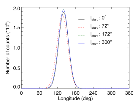
Figure 1: Posterior distributions of four MCMC chains for the longitude of a spot of a model atmosphere. The chains start from different locations in the longitude–space ($l_{start}=[0^{\circ},72^{\circ},172^{\circ},300^{\circ}]$), and we control their convergence using the $\hat{R}$ criterion. For the four chains shown here $\hat{R}\sim$1.01.

We do not include differential rotation or temporal evolution of spots in our code. Modeling light curves that vary from one rotational period to the next in Aeolus we split the light curves in rotational periods and fit every partial light curve separately. We then compare the successive maps and control whether the retrieved variations are physically plausible in the given timeframe.

In the future Aeolus will be modified to fit the inclination and limb darkening of our targets as free parameters. We will also incorporate temporal evolution of features in Aeolus in a physically self–consistent manner.

3 Validating Aeolus on Jupiter

A wealth of information exists on Jupiter’s atmospheric cloud structure and dynamics (see, e.g., Bagenal et al. 2004; de Pater & Lissauer 2010). Atmospheric dynamics and a large number of atmospheric features (e.g., the Great Red Spot (GRS), 5$\mu$m hot spots), indicate that the disk integrated signal of Jupiter varies on the rotational timescale (due to rotational modulations, Karalidi et al. 2013, see, e.g., ) and on much longer timescales (due to atmospheric circulation). Jupiter’s rotational period of 9^hrs55^m27^s.3 (de Pater & Lissauer 2010) is comparable to that of brown dwarfs (see, e.g., Metchev et al. 2015). Clouds in the jovian atmosphere, primarily NH₃ ice (see, e.g., West et al. 1986; Simon-Miller et al. 2001)), are different from the ones predicted in L to T brown dwarfs (sulfide, Mg–silicate, perovskite and corundum clouds) and the first directly imaged exoplanets (see, e.g., Burrows et al. 2006; Marley et al. 2002, 2013). They can be comparable though, to the ones in Y dwarfs (Morley et al. 2014b; Luhman et al. 2014) and cooler giant exoplanets we directly detect in the future. The wealth of variable atmospheric structures, in combination with the ability to get spatially resolved, whole–disk images against which we can compare our maps, makes Jupiter an ideal target for the validation and testing of the sensitivity and limitations of Aeolus.

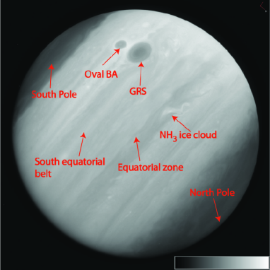
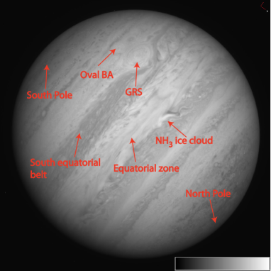
Figure 2: Jupiter imaged in the U–band (top panel) and the R–band (bottom panel) at a phase of $\sim$0.1. The images shown are 1101 x 1101 pixel region extracts from the original 2048 x 2048 pixel imaging detector sub-arrays centred on the planet. For all images, a linear grey-scale display stretch is used with surface brightness encoded as indicated by the scale bars. To optimally tile the full dynamic display range of the data, different display scales (in instrumental units of electrons per pixel) are used for the F275W and F763M images with: F275W–0 (hard black) to 45,000 (hard white) electrons per pixel, F763M– 0 (hard black) to 60,000 (hard white) electrons per pixel. We note that different wavelengths probe different layers in the jovian atmosphere and thus the images differ considerably (see Sect. 3.2).

We applied Aeolus to our Hubble Space Telescope’s (HST) observations of Jupiter. Jupiter was observed with HST Wide–Field Camera 3 (WFC3) in UTC 19-20 September 2012 during 21.5^hrs, i.e., 2.2 jovian rotations. Observations were performed in the F275W and F763M bands. Data acquisition and reduction is further described in Sect. 3.1. With their unprecedented high signal–to–noise ratio (on average, 26,600 in the F275W and 32,800 in the F763M) full disk photometry of Jupiter, combined with high–resolution spatially resolved images over a continuous timespan of more than two jovian days, these observations provide us with a unique dataset. Various Jovian sub-regions have been studied extensively (see, e.g., Simon-Miller et al. 2001; Shetty & Marcus 2010) and a number of full–disk snapshots of Jupiter, Earth and other Solar System planets exist (see, e.g., Smith et al. 1981; Cowan et al. 2009), but to our knowledge there are no previous continuous observations of the full–disk of Jupiter or any other Solar System planets. We applied our mapping code on these unique light curves and compare the derived maps with the HST images of Jupiter.

3.1 HST data & reduction

Time resolved, full disk, photometric UVIS imaging observations of Jupiter, spanning 21.5 hours ($\sim$ 2.2 Jovian rotations), were obtained on UTC 19-20 September 2012 with the HST WFC3 (pixel scale $\sim$40 mas pixel^-1) in HST GO program 13067 (PI: G. Schneider). A total of 124 images were obtained from data acquired in 14 contiguous HST orbits (of $\sim$96 minutes each), sequentially alternating between two spectral filters: F275W (hereafter U–band, $\lambda_{\mathrm{pivot}}$ = 2704${\AA}$, FWHM = 467${\AA}$) and F763M (hereafter R–band, $\lambda_{\mathrm{pivot}}$ = 7612${\AA}$ , FWHM = 704${\AA}$). These data were acquired during, and flanking, a transit of Venus as seen from Jupiter (Pasachoff 2012; Pasachoff et al. 2013a, b), with a predictable maximum photometric depth due to geometrical occultation of $\sim$0.01% (100 ppm), much smaller than the rotation signature from clouds of import to this study. The potential “tall poles” in photometric measurement precision at the levels of possible significance to this investigation are Cosmic Ray (CR) detection and mitigation, instrumental stray light and pointing repeatability. All three are discussed in detail below. We finally corrected our data for the changing Earth–Jupiter and Jupiter–Sun distances, as well as for the changing disk illumination fraction and angular size of Jupiter, over the duration of our observations.

3.1.1 Data acquisition

At the time of these observations, the angular diameter of the nearly fully illuminated (99.03%) disk of Jupiter was $\sim$41.7”. A 2K$\times$2K pixel (80”$\times$ 80”) readout subarray, nominally centered on the planet, was used to reduce readout overheads while also (by its over–sizing) reducing Jovian stray light (encircled energy) escaping the finite imaging aperture field–of–view far from the planet. Exposure times were designed to reach $<$90% full well depth for the brightest features expected in the Jovian cloud tops (to prevent image saturation, we checked against previous imaging) to yield an aggregate $\sim$2.2$\times$10¹⁰ electrons combining all $\sim$866,000 WFC pixels in each image that tiled the disk of Jupiter with exposure times T_exp(u) = 29.40 s and T_exp(r) = 0.48 s. Given expected interruptions in data acquisition from Earth occultations, spacecraft south–Atlantic anomaly (SAA) passages (which vary in orbit phase from orbit to orbit), and the instruments’ occasional need to pause for an image data “buffer dump,” a minimum of six to a maximum of ten images were obtained in each orbit’s approximately 54 minute target–visibility period. When uninterrupted, interleaved intra–image cadences of 225s in U–band, and 214s in R–band, imaging were achieved. Data from the first, and part of the second, HST orbits were (as expected and used for calibration purposes) photometrically partially “corrupted” by excess light from Io intruding into the field of view. Separately, partway through the last (14^th) orbit, the HST pointing control system suffered a guide–star loss–of–lock, degrading the photometric fidelity obtained thereafter. The photometric data set considered in detail in this paper excludes these degraded data, but are inclusive of all others obtained from UTC 01^hrs21^m43^s to 20^hrs27^m46^s. The detailed exposure–by–exposure observing plan is available on-line from the Space Telescope Science Institute.

3.1.2 Basic Instrumental Calibration

The basic (routine) exposure level instrumental calibration of the raw imaging data (data set identifier IC3G* in the Mikulski Archive for Space Telescopes (MAST)) including gain conversion, bias, dark current corrections and flat fielding, was done using STScI’s calwfc3 calibration software (as implemented in the HST OPUS pipeline). As these raw data were acquired without a need for post–flashing (due to the bright-target field), no post–flash corrections were performed. Because Jupiter is both a moving, and spatially–resolved rotating target, and data extraction at the full sampling cadence was desired, the individual FLT, not DRZ (“drizzle” combined) files were used in subsequent post–processing and photometric analysis.

3.1.3 Astrometric Image Co–Alignment

Small (few pixel) image offsets were noted in observed images, even those using the same guide stars, likely mostly due to imperfections in moving–target tracking. Comparable offsets were seen between visits (orbits) where changes in the secondary guide stars was required due to the planetary motion. For each filter, all differentially imperfectly pointed images were astrometrically co–aligned (registered) prior to the identification and subsequent correction of CR affected pixels, and for later large, enclosing aperture, photometry. Differential image decentrations were determined from sequential image pairs by minimizing the variance in a small (few pixel) width annulus enclosing the limb of Jupiter in difference images with iterative “shifting” of the image treating ($\Delta$x, $\Delta$y) as free parameters. “Shifting” (with each iteration re–referenced to the original image) was done by sub–pixel image remapping via bi–cubic interpolation apodized by a sinc function of kernel width appropriate to each filter to suppress ringing. The then astrometrically co–registered FLT files were not additionally corrected for the WFC3 geometrical distortion, which is actually preferable to omit for high–precision differential photometry in obviating additional flux-density interpolation errors in geometrical correction associated pixel remapping. (N.B.: This is why, by chance of observational geometry/spacecraft orientation, geometrically uncorrected FLT images of Jupiter look quite round, rather than oblate, as exampled in Fig. 2).

3.1.4 Cosmic Ray rejection

Although exposure times (and so susceptibility to CR hits) are small, (multiple) high–energy CR events could photometrically bias even large-aperture photometry if not at least partially mitigated by CR detection and compensation Since Jovian image structure is not static, the simple oft–used two–image minimum, or multiple, image median approach for intrinsically invariant images is not appropriate. Here we adopted a hybrid approach, different in process for the sky background region (which includes instrumentally scattered planetary light, so is necessary to correct and later photometer) and for the planetary disk. On disk we use local median spatial filtering, and off–disk we use simple image–pair anti–coincidence detection.

The on–disk region has spatially and temporally variable cloud structure that, even on small spatial scales, has detectable changes from image to image at WFC3 resolution even at the shortest sampling timescales. Most of these are correlated in two dimensions over at least several pixels, whereas CR hits are usually isolated to single pixels or are “trails” only one pixel in width. Thus, we identify most CR–affected pixels as outliers identified from high–pass spatially–filtered images. Spatial filtering is simply done, for each image, by subtracting a 3$\times$3 pixel boxcar image convolution of the image from image itself. On–disk CR–corrupted pixels are then identified from the spatially–filtered images as $\geq$+3.5$\sigma$ outliers w.r.t. 1$\sigma$ deviations in an on–disk 700$\times$700 pixel planet–centered sub–array fully circumscribed by the disk of Jupiter. (In detail, with experimentation using different size filtering kernels we found in the 3$\times$3 case $<$3$\sigma$ erroneously finds pixels that are correlated with disk structure, and $>$ 4$\sigma$ “misses” many uncorrelated pixels (tested by injecting CR–like signals into template images). While the surface brightness of the disk is locally variable, a constant 3.5$\sigma$ threshold w.r.t. the (centrally brighter) 700$\times$700 pixel disk–centered subarray provides a statistically uniform clipping (identification) level w.r.t. CR energy (intensity) for all images (in each filter). For the full ensemble of U and R images, respectively, the medians of the 1$\sigma$ deviations in the central 700$\times$700 pixel regions are uniformly adopted to establish the clipping threshold for all like–filter images: U_median(1$\sigma$) = 212.6 counts/pixel, R_median(1$\sigma$) = 255.6 counts/pixel (compare full–disk averaged signal levels $\sim$30,000 counts/pixel and $\sim$2.2E10 counts integrated over the full disk of Jupiter.

Off–disk (sky) CR–compromised pixels are found (to a limiting threshold) in a two–step process. Step 1: In each visit, sequential image pairs in the same filter are inter–compared to find the smaller–valued of two co–located pixels (for all sky pixels) with the presumption of intrinsic background sky image stability between same–filter sequential images. In the absence of CR events (and sky instability) the sky–region images will differ significantly only by instrumental noise plus photon noise in the background. The smaller–valued of each of the two–pixel pairs is used to assess the sky background at that pixel location. Step 2: In infrequent cases where independent CR–events may pollute the same pixel in sequential images this method will fail to find a proper sky estimation for that pixel. Those pixels are then identified by sigma–clipping against the local background after pixel–pair minimization. The spatially mutually–exclusive on and off disk regimes are then re–combined to produce a “CR cleaned” image to the above detection threshold limits.

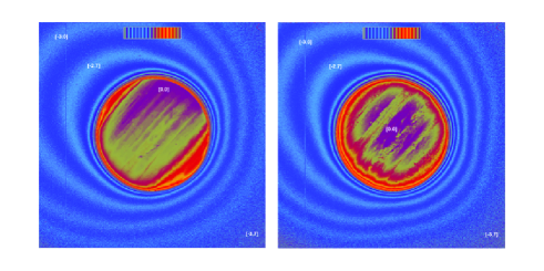
Figure 3: Representative circumplanetary stray/scattered light. Left: U-band, Right: R-band. Log 10 display normalized to peak on–disk intensity. $+3.3$% isophotes in log10 space from [-4] to [0] dex counts/pixel.

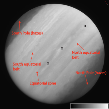
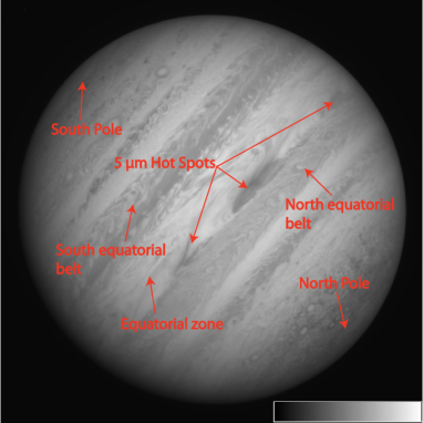
Figure 4: U–band (top panel) and R–band (bottom panel) Jupiter snapshot at a phase angle of $0.3$. We note that the 5 $\mu$m hot spots we see in the R–band have no visible counterpart in the U–band (locations marked with X). Colorbars as in Fig. 2.

3.1.5 Instrumental (Stray) Light and HST Pointing Authority in Detail

Instrumentally scattered light from the large, bright, disk of Jupiter into the circumplanetary sky background is both circularly asymmetric and falls off much more slowly (as expected) than the PSF halo of an isolated point source. This is shown illustrated in Fig 3 for representative F275W and F763M brightness maps shown as contour images log10 stretched normalized to the surface brightness of the brightest parts of the Jovian disk. As can be seen, at the edge of the FOV the “sky” brightness from Jovian stray light has declined to only $\sim 10^{-3}$ to $10^{-4}$ of the peak surface brightness of the disk. (The full dynamic display range in this image display is [-4] to [0] dex relative to the brightest parts of the disk).

The ability to achieve high–precision source–enclosing large–aperture (including sky) differential photometry depends, then, upon the stability of the stray light pattern, i.e., if the planet moves in the 2k$\times$2k imaging subarray between exposures, the stray light pattern will shift. Its structure may then change resulting in different amounts of stray light falling out of the photometric aperture used, not only because of decentration (that is post–facto compensated; see Astrometric Image Co–Alignment), but from a possible change in the two–dimensional structure of the scattered light pattern with target displacement in the FOV. HST pointing stability while using two Fine Guidance Sensor fine lock guiding (used for these observations) with respect to the planetary tracking precision is approximately 4 mas RMS. Target re–acquisition precision, with the same guide stars in successive orbits, is $\sim$10 mas or better from visit to visit. Fortuitously, the same primary guide star (which is used for attitude control) was available and used for all 14 visits. Because of Jupiter’s motion through the sky, however, the observing program switched twice to different secondary guide stars (which are used for roll control). Re–using the same primary guide star for all visits should (to close to first order) result in the target (center of Jupiter) placement in the aperture very repeatable in all visits, but a small differential roll error (tenths of a degree) between Visits 07 and 08, and again Visits 12 and 13, when the secondary guide stars were switched, could potentially bias the aperture photometry (with an undersized aperture) – but is not seen in these data when reduced (masking aperture edges) and measured.

3.2 Phenomenological analysis of Jupiter images

Identifying the most prominent features in Jupiter’s U– and R–band images is important for interpreting the jovian light curves and controlling the validity of our mapping technique. In Fig. 2 we present a Jupiter snapshot in the U (top panel) and R (bottom panel) bands at a rotational phase angle of $\sim$0.1. Note that the images are oriented with the South pole located on the upper left corner of the images.

Even though the two images are taken at the same rotational phase angle they differ considerably. In the U–band the jovian disk is nearly homogeneous (jovian zones and bands appear smooth and of comparable intensity) and the most prominent features are the Great Red Spot (GRS) and Oval BA (see Fig. 2). Additionally, the jovian poles appear darker than the central parts of the disk. On the other hand, in the R–band the GRS and Oval BA disappear, i.e., they have the same color and intensity as the South temperate belt. The jovian disk appears clearly heterogeneous due to the prominent zones and belts, while the poles appear darker due only to limb darkening. This is due to the different atmospheric layers probed at the two wavelengths.

In particular, the short–wavelength U–band probes the higher jovian atmosphere down to $\sim$400 mbar (Vincent et al. 2000), and we can observe the GRS (top pressure of $\sim$250 mbar) and the Oval BA (top pressure $\sim$220 mbar) (Simon-Miller et al. 2001). The zones and belts, on the other hand, have cloud-top pressures of 600 mbar down to 1 bar (Simon-Miller et al. 2001), making them visible at the longer wavelength (R–band) observations, which probes deeper pressure levels in the atmosphere down to $\sim$2 bars (Irwin 2003).

Stratospheric hazes cover Jupiter’s poles (at pressures of 10–100 mbar), consisting of aggregates of particles that are small in comparison to the incident light (West & Smith 1991; Ingersoll et al. 2004). These hazes are thought to be condensed polycyclic aromatic hydrocarbons or hydrazine, generated in the upper stratosphere from CH₄ under the influence of the solar ultraviolet radiation (Friedson et al. 2002; Atreya et al. 2005). Due to their high altitude we expect the polar hazes to be visible in the U–band observations and not in the R–band. Additionally, we expect them to appear darker than the background NH₃ clouds (e.g., Karalidi et al. 2013, their Fig.1), as we indeed see in Fig. 2.

Jupiter’s GRS is located at a latitude of $22.4^{\circ}\pm 0.5^{\circ}$S, with a latitudinal extent of $11^{\circ}\pm 1^{\circ}$ (Simon-Miller et al. 2002) and a longitudinal extent of $18.07^{\circ}\pm 0.91^{\circ}$ as of 2000 (Trigo-Rodriguez et al. 2000; Simon-Miller et al. 2002), which given a linear shrinkage rate of $-0.114^{\circ}/\mathrm{yr}$ (Simon-Miller et al. 2002), would translate to $16.70^{\circ}\pm 0.91^{\circ}$ in 2012. Oval BA is located at $33^{\circ}$S latitude (Wong et al. 2011), and extends $\sim 5^{\circ}$ in latitude and $\sim 11^{\circ}$ in longitude (Shetty & Marcus 2010, Fig.18).

In Fig. 4 we present Jupiter at a phase angle of 0.3. In the R–band (right panel) we notice the existence of a large hot spot on the North hemisphere. In hot spots, the atmospheric cloud content is low and the heat can escape from deeper layers without much absorption. Hot spots thus appear dark in the visible, but bright at 5$\mu$m (Vasavada & Showman 2005). Jupiter’s hot spots are centered around $6.5^{\circ}$N–$7^{\circ}$N latitude (Ortiz et al. 1998; Simon-Miller et al. 2001). Their longitudinal to latitudinal extent ratio varies between 1:1 to 7:1, while strong zonal flows at the north and south boundaries of these features limit their latitudinal size to a maximum of $8^{\circ}$ (Choi et al. 2013). The hot spot of Fig. 4 has a latitudinal extent of $\sim 4^{\circ}$ and a longitudinal extent of $\sim 18^{\circ}$.

3.3 Light curve inspection

In Fig. 6 we present the normalized R (red boxes) and U (blue circles) band HST light curves of Jupiter. Before testing our mapping code we inspected the light curves and compared them with the HST images of Jupiter.

The R–band light curve has a peak–to–peak amplitude of $\sim$2.5% and appears to be a smooth sinusoidal function. In comparison, the U–band light curve has a small peak–to–peak amplitude of $\sim$0.5% and its small scale structure indicates that it is influenced by multiple atmospheric structures.

A comparison of the R–band light curve with HST images shows that the hot spot of Fig. 4 (left panel) is responsible for the troughs of the light curve (see also Fig. 6), while the GRS for the peaks. In the U–band the GRS and Oval BA (see right panel of Fig. 4) appears to be responsible for the lower flux around a phase of 0.9 and 1.8, while the overall small–scale structure seems to be due to changes in the distribution of high NH₃ ice clouds (see also Fig. 6).

We define as $0^{\circ}$ longitude the center of the first image acquired during these HST observations. In Fig. 5 (top panel) we show a latitudinal flux profile of Jupiter at a longitude of $\sim 334^{\circ}$, passing through the GRS and Oval BA (red, dashed–dotted line) and at a longitude of $\sim 116^{\circ}$ (black, solid line). The GRS and Oval BA (around a latitude of $-23^{\circ}$ and $-34^{\circ}$ respectively) are darker than their surrounding TOA. In particular, the GRS at its darker part has a contrast ratio of 0.55 (0.62) to the disk at its north (south) side and Oval BA has a contrast ratio of 0.70 (0.79) to the disk at its north (south) side (see bottom panel of Fig. 5). Full disk photometry of our images though shows that Jupiter’s GRS has a contrast ratio of 0.97 to the integrated background jovian disk (as seen in the U–band) and the Oval BA has a contrast ratio of 1.17. This is due to the extremely dark poles of Jupiter in the U–band. Finally, the big hot spot we see in the left panel of Fig. 4 has a contrast ratio (as seen in the R–band) of 1.15.

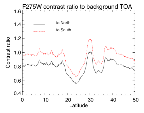
Figure 5: Top: Jupiter latitudinal U–band flux profiles at a longitude of $\sim 116^{\circ}$, not passing through the GRS and Oval BA (black, solid line) and of $\sim 320^{\circ}$, passing through the GRS and Oval BA (red, dashed–dotted line). We define as $0^{\circ}$ longitude the center of the first image acquired during these HST observations. We notice that the GRS and Oval BA are darker than their directly surrounding disk. Bottom: Contrast ratio of a slice of the top figure to a location to the North ($\sim$-17^∘; black, solid line) and to the South ($\sim$-29^∘; red, dashed–dotted line) of the GRS.

3.4 Application of Aeolus

We initially applied Aeolus to Jupiter’s R–band light curve. We ran $8$ chains of length 5,000,000 each, with different initial conditions. We used the Gelman and Rubin (R̂) criterion to test our chains’ convergence. Since the light curve shows evolution from one rotation to the next, we split it and ran our MCMC code on each rotation ($10^{\mathrm{hr}}$ intervals) separately.

For the first rotation, we retrieved 2 spots (BIC 19.3) located at a longitude of $128.8^{\circ}\pm 12.8^{\circ}$ and $312^{\circ}\pm 10^{\circ}$; a latitude of $23^{\circ}\pm 12^{\circ}$ and $31^{\circ}\pm 16^{\circ}$; with a size of $16.7^{\circ}\pm 1.8^{\circ}$ and $18^{\circ}\pm 4^{\circ}$; and a contrast ratio of $0.96\pm 0.20$ and $1.2\pm 0.2$. For the second rotation, we retrieved 2 spots (BIC 15.6), located at a longitude of $126^{\circ}\pm 15^{\circ}$ and $315^{\circ}\pm 14^{\circ}$; a latitude of $22^{\circ}\pm 12^{\circ}$ and $31^{\circ}\pm 16^{\circ}$; with a size of $18^{\circ}\pm 3^{\circ}$ and $18^{\circ}\pm 4^{\circ}$; and a contrast ratio of $1.04\pm 0.18$ and $1.2\pm 0.2$. The Aeolus–retrieved spot properties are, within the error bars, in agreement with the properties of the hot spot and the GRS as presented in Sect. 3.2. For completeness, in Fig. 7 we show the normalized R–band light curve (red triangles) with error bars, and the best fit Aeolus model (black, solid line) for the first rotation (top panel), and the residuals (bottom panel).

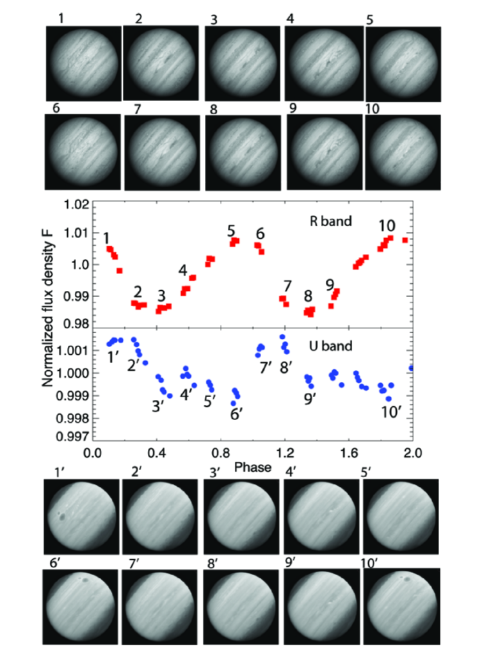
Figure 6: Normalized R (red) and U (blue) band light curves of Jupiter. The uncertainties in the relative, disk–integrated, photometric measures (each point) are estimated as 1$\sigma\leq$ 0.022%$\pm$0.009% of the measured signal in either filter band. Corresponding snapshot images of Jupiter in the R–band (top) and U–band (bottom) are shown for helping the reader interpret the light curves.

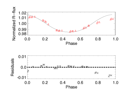
Figure 7: Normalized R–band light curve of Jupiter (red triangles) with error bars, and best fit Aeolus curves (black solid line) for the first rotation (top panel); and corresponding residuals (bottom panel).

We then applied Aeolus to Jupiter’s U–band light curve. The U–band light curve has a smaller amplitude and its temporal evolution is more pronounced than that of the R–band. We again split the curve into two rotations and fit each curve separately.

For the first rotation, Aeolus retrieved 1 spot (BIC 24.5 vs 28.7 for two spot model) located at a longitude of $290^{\circ}\pm 20^{\circ}$ and a latitude of $24^{\circ}\pm 8^{\circ}$, with a size of $19.6^{\circ}\pm 2.1^{\circ}$ and a contrast ratio of $1.05\pm 0.08$ to the background. For the second rotation, Aeolus retrieved 1 spot (BIC 19.1) located at a longitude of $319^{\circ}\pm 14^{\circ}$ and a latitude of $13^{\circ}\pm 7^{\circ}$, with a size of $20.0^{\circ}\pm 1.0^{\circ}$ and a contrast ratio of $1.22\pm 0.14$ to the background. Within the error bars, our retrieved spot properties agree with the GRS properties as presented in Sect 3.2. Note that the latitudinal location and size of the retrieved GRS are slightly offset, due to the influence of the Oval BA.

The error in the estimated latitude is large (relative to the mean). This is due to the latitudinal degeneracy maps based on flux observations present (see, e.g., Apai et al. 2013). As expected, rotationally homogeneous features such as the belts and zones of Jupiter do not leave a clear trace in the light curves (see, e.g., Karalidi et al. 2013). Finally, we note that the Oval BA accompanying the GRS cannot be retrieved as a separate feature by Aeolus, which is again due to the latitudinal degeneracies.

We should note here, that Aeolus had difficulties converging, given the very small uncertainties of our Jovian light curves. Aeolus was designed to reproduce simple surface brightness maps of ultracool atmospheres, assuming that all heterogeneities on the TOA are elliptical. A closer look at the U–band light curves of Fig. 7 though, indicates that due to the high SNR ratio of our dataset, the light curve shape is also influenced by non–elliptical, fine structures, such as high NH₃ ice clouds. Since the modeling of such fine structure is beyond our scope and Aeolus’ design, and for achieving fast convergence, we increased $\sigma$ by a factor of $\sim$4. Doing so, we kept $\sigma$ well below the uncertainties of the highest–precision brown dwarf observations (see, e.g., Apai et al. 2013; Yang et al. 2015), and allowed Aeolus to map the major non-rotationally–symmetric features of Jupiter in the U– and R–bands.

3.4.1 Fourier mapping of Jupiter

We then compared Aeolus maps with those produced using Fourier mapping, a commonly used mapping technique in the literature. Following Cowan & Agol (2008), and given that our problem was under–constrained, we defined the longitudinal brightness map of any planet as: $M(\alpha)=\frac{a_{0}}{2}+\frac{2b_{1}}{\pi}\cos(\alpha)-\frac{2c_{1}}{\pi}\sin(\alpha)+\frac{3b_{2}}{2}\cos(2\alpha)-\frac{3c_{2}}{2}\sin(2\alpha)$, where $\alpha$ is the angle of rotation of Jupiter or a brown dwarf around its axis.

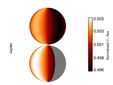
Figure 8: Fourier surface brightness map of Jupiter based on its U–band, first rotation. Upper panel: map centered at a longitude of $140^{\circ}$. Lower panel: map centered at a longitude of $320^{\circ}$. Grey areas correspond to missing data due to an Europa intrusion.

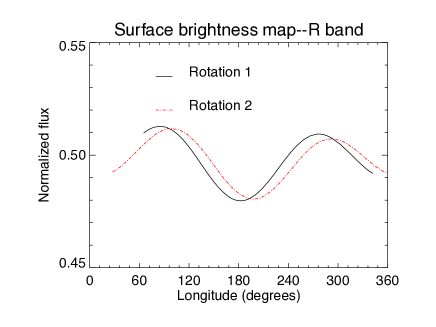
Figure 9: Fourier surface brightness map of Jupiter based on its U (top) and R (bottom) bands, based on the first (black, solid lines) and the second (red, dashed–dotted lines) rotation.

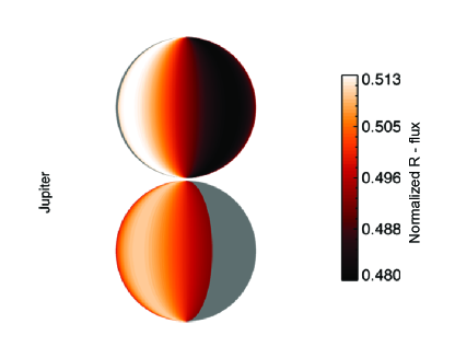
Figure 10: Fourier surface brightness map of Jupiter based on its R–band, first rotation. Upper panel: map centered at a longitude of $140^{\circ}$. Lower panel: map centered at a longitude of $320^{\circ}$.

Fig. 8 to 10 show the longitudinal brightness maps of Jupiter in the U– and R–bands. As discussed in Sect. 3.4, we split the light curve for the two rotations and mapped each one separately. Fig. 8 and 10 show the map of the first rotation and, for comparison, Fig. 9 shows the map of both rotations in the U (top panel) and R (bottom panel) bands. We ignored the first four snapshots of Jupiter due to an Europa intrusion, resulting in the first rotation maps (black lines of Fig. 9) starting at $\sim$40 (rotational phase angle of $\sim$0.1).

In the U–band, features appearing in the map of the first rotation appear in the map of the second rotation as well, albeit with a different longitudinal size. The retrieved intensities of features in the second rotation are slightly higher than those of the first rotation. This is due to a slight increase ($\sim$0.03%) in the normalized flux of the second rotation in comparison to the first rotation (see Fig. 6). In the R–band the maps of the two rotations are of equal brightness, but slightly offset.

Comparing the U–band maps with Jupiter HST images, we notice that the dark area around $\sim$340^∘ of longitude coincides with the location of the GRS and Oval BA on the disk. In the first rotation map, the dark region appears broad and incorporates longitudes coexisting with the GRS and Oval BA on the HST snapshots. In the second rotation, the dark region appears at longitudes $\lesssim 60^{\circ}$ and $\gtrsim 340^{\circ}$, incorporating longitudes coexisting with the GRS and Oval BA on the HST snapshots. The brightening around a longitude of $250^{\circ}$ could be related to a white plume appearing in the jovian disk. White plumes are thought to be the result of upwelling NH₃ clouds that freeze, resulting in high altitude fresh ice cloud (Simon-Miller et al. 2001). Finally, the darker area around $180^{\circ}$ corresponds to a featureless jovian disk.

Comparing the R–band maps with the HST images, we notice that the brighter area around a longitude of $\sim$100^∘ corresponds to the snapshots in which the big hot spot is visible. The darker area around a longitude of 200^∘ corresponds to snapshots in which smaller hot spots are visible on the disk. Finally, the brightening of the disk around 300^∘ corresponds to images where the GRS appears on the disk (remember that as mentioned in Sect. 3.2 the GRS cannot be seen in the R–band, but appear as areas of equal brightness to the southern temperate belt).

3.5 A modified Jupiter

To test Aeolus, we simulated a Jupiter–like planet with extra spots at various locations and various sizes and contrast ratios and retrieved the maps of these “modified” Jupiters. In Table 1 we summarize the various spot locations used.

Table 1: Test cases for Aeolus. To test the sensitivity of Aeolus we simulated a modified Jupiter with two spots at various longitudinal (l) and latitudinal ($\phi$) distances between them. The spot size and contrast ratio to the background TOA was kept constant for every set of simulations.

Test case	l1(deg)	l2(deg)	$\phi_{1}$(deg)	$\phi_{2}$(deg)
1	130	[145,149,154,164,174,184,204,224]	0	0
2	130	280	0	[0,30,60]
3	130	130	0	[20,30,50,80]
4	343	N/A	[0,30,50,60,80]	N/A

Initially, we simulated an atmosphere with two spots located at the equator and varied the longitudinal distance between them (see Table 1), to study the longitudinal sensitivity of our mapping code. We placed one spot at $l=130^{\circ}$, with a size of $s=18^{\circ}$ and a contrast ratio of 0.7, while the second spot had a size of $10^{\circ}$ and a contrast ratio of 0.4. In Table 2 we show the number of spots retrieved from Aeolus, its corresponding BIC, and whether the retrieved properties are (within the error bars) in agreement with the input properties or averaged between the two spot properties. For longitudinal spot separations (center to center) up to $34^{\circ}$, Aeolus retrieved 1 spot with average properties, while for larger separations, it retrieved 2 spots with properties that agreed, within the error bars, with the input properties. As an example, Fig. 11 (upper half) shows the input map (left column) and the corresponding Aeolus retrieved map (right column) for test cases 1c (first row) and 1g (second row). For clarity, we plot the maps centered at 130^∘ longitude.

We then placed the second spot at a longitude of $280^{\circ}$ and varied its latitude (see Table 1). We set the spot size equal to $20^{\circ}$ and contrast ratio to the background to $0.4$. Aeolus retrieved 2 spots, whose longitude and size were, within the error bars, in agreement with the input properties (see Table 2). The latitudinal location and contrast ratio of the spots were retrieved slightly offset from the input values.

We then modeled an atmosphere with one spot at a longitude of 130^∘, a latitude of $0^{\circ}$, a size of $s=18^{\circ}$, and a contrast ratio of 0.7; and a second spot at the same longitude (130^∘), and varied its latitude (see Table 1). We set the second spot’s size to 10^∘ and contrast ratio to the background at 0.4. Aeolus retrieved 1 spot with all properties averaged (Table 2). As an example, Fig. 11 (bottom half) shows the input map (left column) and the corresponding Aeolus retrieved maps (right column) for test cases 3a (third row), and 3d (fourth row). We note that the closer the second spot was to the pole, the closer the retrieved properties were to the equatorial spot’s properties. We observed a similar behavior when mapping Jupiter based on its U–band light curve (Oval BA cannot be retrieved). This is due to a degeneracy among models with spots at different latitudes and with different contrast ratios/sizes when flux (without polarization) measurements are taken into account. We will discuss this problem further in Sect 5.

We finally modeled an atmosphere with one spot, at a longitude of $343^{\circ}$, with a size of $s=27^{\circ}$ and a contrast ratio of 0.87, and varied its latitude through the following values: $0^{\circ}$, $30^{\circ}$, $50^{\circ}$, $60^{\circ}$ and $80^{\circ}$. Fig. 12 shows the latitude of the spot for the five test cases (red squares), and the corresponding latitudes Aeolus retrieved (black triangles), with error bars. Aeolus retrieved the variation of the spot’s latitude between our test cases, demonstrating the two–dimensionality of Aeolus maps. We also tested the effect that an error in the estimated rotational period has on the retrieved maps. We varied the estimated rotational period by up to 10% and compared the maps Aeolus retrieved with those retrieved when the rotational period is known accurately. We found that the retrieved maps are in agreement ($\Delta l_{max}\sim$0.49%, $\Delta\phi_{max}\sim$0.78%, $\Delta s_{max}\sim$ 0.66%, $\Delta f_{max}\sim$1.19%), indicating that small uncertainties in the rotational period do not have a major impact on Aeolus maps.

Table 2: Aeolus results for test cases of Table 1.

Test case	# spots	BIC	Retrieved properties
1 (a) to 1 (d)	1	16.4	averaged
1 (e) to 1 (h)	2	15.4 to 17.04	in agreement
2	2	16.5	in agreement
3	1	15.5 to 16.4	averaged
4	1	16.2 to 20.	in agreement

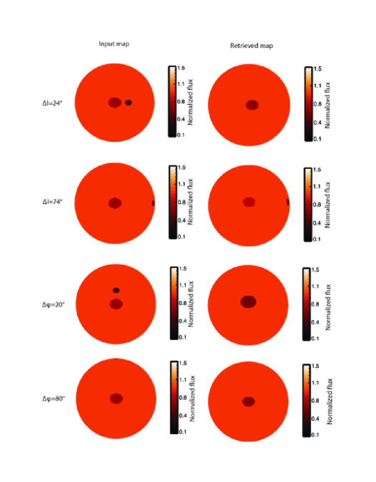
Figure 11: Sample of input (left column) and Aeolus retrieved maps (right columns), for test cases:1c (first row), 1g (second row), 3a (third row) and 3d (fourth row). For clarity we show the maps centered at 130^∘ longitude.

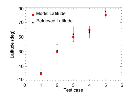
Figure 12: Latitude of the spot of five model atmospheres (red squares), and corresponding Aeolus retrieved latitudes (black triangles), with error bars. In high quality data Aeolus can correctly identify the latitude of the elliptical features.

4 Brown dwarfs

Temporal variations in brown dwarf brightnesses indicate that their atmospheres present complex cloud structures (Apai et al. 2013). Here we applied Aeolus to map two rotating brown dwarfs in the L/T transition, 2MASSJ0136565+093347 (hereafter SIMP0136) and 2MASSJ21392676+0220226 (hereafter 2M2139). We used observations that were taken by Apai et al. (2013) using the G141 grism of the Wide Field Camera 3 on the Hubble Space Telescope (Project 12314, PI: Apai). These observations provide spatially and spectrally resolved maps of the variable cloud structures of these brown dwarfs. For a detailed description of the data acquisition and reduction, we refer the reader to Apai et al. (2013). Apai et al. (2013) performed synthetic photometry in the core of the standard J– and H– bands.

In Fig. 13 we show the period–folded H (red blocks) and J (green circles) light curves of 2M2139 (top panel) and SIMP0136 (lower panel). Both 2M2139 and SIMP0136 exhibit brightness variations in the H– and J–bands, with peak–to–peak amplitudes of 27% and 4.5% respectively. Both targets’ light curves vary in a similar manner, independent of the observational wavelength. Given that as previously discussed (Sect. 3.2), different wavelengths probe different pressure layers, the similar appearance of 2M2139 and SIMP0136 in the H– and J–bands indicates a similar TOA map for the different pressure levels.

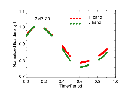
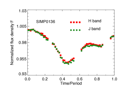
Figure 13: Period folded H(red blocks), and J (green circles) light curves of 2MASSJ21392676+0220226 (top panel) and 2MASSJ0136565+093347 (lower panel).

4.1 2M2139

2M2139 is classified as a T1.5 by Burgasser et al. (2006) based on NIR observations. Later observations suggested 2M2139 could be a binary composite of an L8.5$\pm$0.7 and a T3.5$\pm$1.0 based on SpeX spectra (Burgasser et al. 2010), even though a spectral modeling study by Radigan et al. (2012) reached a different conclusion and high–resolution HST observations detected no evidence for a companion (Apai et al. 2013). Ground–based photometry of 2M2139 suggested light curve evolution on timescales of days, indicating a considerable evolution of cloud cover in its atmosphere (Radigan et al. 2012). Radigan et al. (2012) observed a very large variability of up to $26\%$ in the J–band and a period of 7.721$\pm$0.005 hr. Apai et al. (2013) carried out time–resolved HST near–infrared spectroscopy that covered a complete rotational period. This dataset showed that rotational modulations are gray, i.e. only weakly wavelength–dependent. State–of–the–art radiative transfer modeling of the color–magnitude variations demonstrated that the changes are introduced by cloud thickness variations (warm thin and cool thick clouds). PCA analysis showed that $>99\%$ of the spectral variations can be explained with only a single principal component, arguing for a single type of cloud feature (Apai et al. 2013). Light curve modeling found that three–or–more–spot models are needed to explain the observed light curve shapes.

4.2 SIMP0136

SIMP0136 is a T2.5 dwarf (Artigau et al. 2006), with a period of 2.3895$\pm$0.0005 hr and exhibits peak to peak variability of up to 4.5$\%$ in the J– and H– bands (Artigau et al. 2009). SIMP0136 shows a significant night-to-night evolution (Artigau et al. 2009; Apai et al. 2013; Metchev et al. 2013) even though it does not appear to be a binary (Goldman et al. 2008; Apai et al. 2013). Time-resolved HST near-infrared spectroscopy by Apai et al. (2013) found that the observed variations of SIMP0136 are nearly identical to those observed in 2M2139 and are also interpreted by a combination of thin clouds with large patches of cold and thick clouds.

4.3 Comparison of Aeolus with Fourier and PCA maps of 2M2139 and SIMP0136

We applied Aeolus to the light curves of Fig. 13 and compared the retrieved maps of 2M2139 and SIMP0136 with the corresponding maps using Fourier decomposition and with Stratos maps produced by Apai et al. (2013).

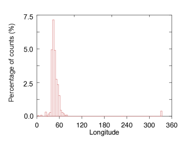
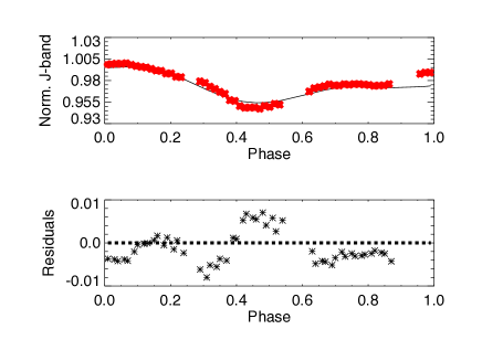
Figure 14: Posterior distribution for the longitude of spot 1 of 2M2139 (top panel); normalized J–band light curve of 2M2139 (red triangles) with error bars and best-fit Aeolus light curve (black, solid line) (middle panel); and residuals (bottom panel).

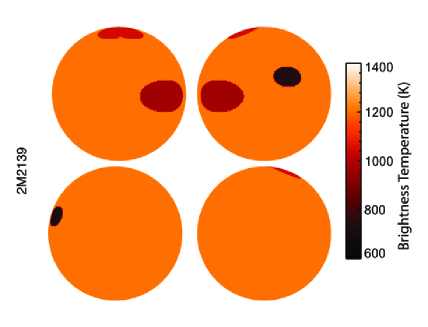
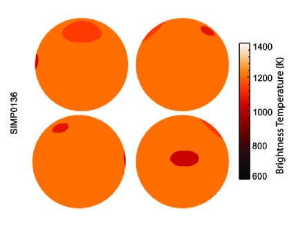
Figure 15: 2M2139 (top four maps) and SIMP0136 (bottom four maps) brightness temperature maps from applying Aeolus on the J band light curves of Fig. 13. The maps are centered at $0^{\circ}$ of longitude (upper left map), $90^{\circ}$ of longitude (upper right map), $180^{\circ}$ of longitude (lower left map) and $270^{\circ}$ of longitude (lower right map).

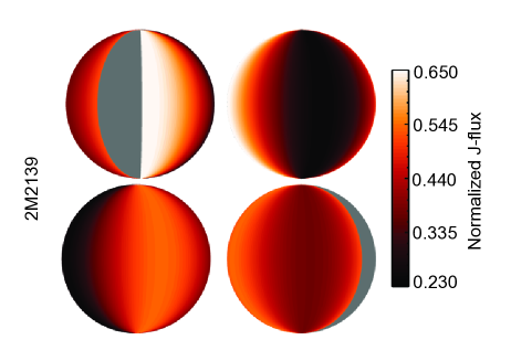
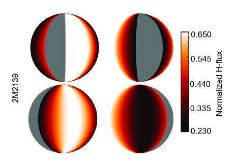
Figure 16: 2M2139 Fourier maps from the J (top four maps) and H (bottom four maps) band centered at $0^{\circ}$ (top left), $90^{\circ}$ (top right), $180^{\circ}$ (bottom left) and $270^{\circ}$ (bottom right) longitude. Dark grey indicates areas without data (due to the lack of data points above a rotational phase of 0.9).

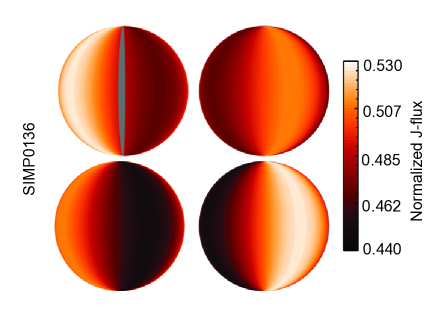
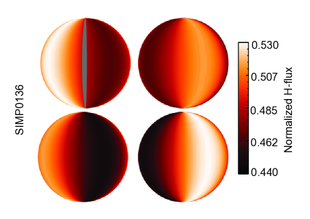
Figure 17: Same as Fig. 16 but for SIMP0136.

Initially, we applied Aeolus to the 2M2139 light curves of Fig. 13. Fig. 14 shows the posterior distribution of the longitude of spot 1 (top panel); the normalized J–band light curve (red triangles) with error bars and best-fit Aeolus light curve (black, solid line) (middle panel); and the corresponding residuals (bottom panel). Based on the J–band light curve, Aeolus retrieved 3 spots (BIC 30) with (longitude, latitude) = ($111^{\circ}\pm 15^{\circ}$, $15^{\circ}\pm 10^{\circ}$), ($45^{\circ}\pm 5^{\circ}$, $2^{\circ}\pm 10^{\circ}$) and ($344^{\circ}\pm 10^{\circ}$, $77^{\circ}\pm 15^{\circ}$), with respective sizes of $13^{\circ}\pm 3^{\circ}$, $27^{\circ}\pm 4^{\circ}$ and $39^{\circ}\pm 5^{\circ}$ and contrast ratios of $0.18\pm 0.10$, $0.57\pm 0.07$ and $0.79\pm 0.04$. A similar map was retrieved based on the H–band light curve.

We then applied Aeolus on the SIMP0136 light curves of Fig. 13. Based on the J–band light curve, Aeolus retrieved 3 spots (BIC 51) with (longitude, latitude) = ($272^{\circ}\pm 21^{\circ}$, $4^{\circ}\pm 7^{\circ}$), ($143^{\circ}\pm 20^{\circ}$, $47^{\circ}\pm 17^{\circ}$) and ($0^{\circ}\pm 5$, $49^{\circ}\pm 15^{\circ}$), with respective sizes of $18.57^{\circ}\pm 2.6^{\circ}$, $17^{\circ}\pm 2^{\circ}$ and $37.5^{\circ}\pm 1.8^{\circ}$ and contrast ratios of $0.77\pm 0.07$, $0.87\pm 0.18$ and $1.12\pm 0.05$. A similar map was retrieved based on the H–band light curve.

In summary, Aeolus found that both 2M2139 and SIMP0136 are covered by three spots, with a longitudinal coverage of 21%$\pm$3% and 20.3%$\pm$1.5% respectively (see Fig. 15).The size of the larger spot in 2M2139 was found to be $39^{\circ}\pm 11^{\circ}$ and in SIMP0136 $37.5^{\circ}\pm 1.8^{\circ}$. 2M2139’s spots are darker than the background TOA, while SIMP0136 has two dark and one brighter than the background TOA spots. Assuming that brightness variations across the TOA are due to the different temperature of the areas observed, we can calculate the brightness temperature variations across the TOA. This would be, for example, the case when due to thinner clouds we see deeper, hotter layers of the atmosphere. In Fig. 15 we show 2M2139 and SIMP0136 brightness temperature maps, assuming the background TOA has a brightness temperature of 1100 K (following Apai et al. 2013). The darkest spot of 2M2139 is $\sim 380$ K cooler and its brightest spot is $\sim 63$ K cooler than the background TOA. SIMP0136’s darkest spot is $\sim 70$ K cooler than the background TOA, while its brightest spot is $\sim 32$ K hotter than the background TOA.

We then applied the Fourier mapping technique to the light curves of Fig. 13. Figs. 16 and 17 show the maps of 2M2139 and SIMP0136 respectively, in the J (top panel) and H (bottom panel) bands. As expected from the similarity of the light curves, the retrieved maps look similar in the two wavelengths.

The J-band surface brightness map for 2M2139, relative to the global average, is bright for $280^{\circ}\lesssim l\lesssim 330^{\circ}$, and dark for $30^{\circ}\lesssim l\lesssim 100^{\circ}$ and $140^{\circ}\lesssim l\lesssim 230^{\circ}$. A brightening around $120^{\circ}$ corresponds to a bump in the light curve around a phase of 0.4. Given the amplitude of the flux increase (0.6% with respect to a sinusoidal fit) and the uncertainty of 0.04%, we conclude that this bump is due to an actual feature in the brown dwarf atmosphere. 2M2139’s H–band map is similar to its J–band map but heterogeneous features appear less bright and narrower (by $\sim 10^{\circ}$) than their J–band counterparts. These differences can be traced back to the differences in the H and J band light curves of Fig. 13.

The J-band surface brightness map for SIMP0136, relative to the global average, is bright for $40^{\circ}\lesssim l\lesssim 70^{\circ}$ and $220^{\circ}\lesssim l\lesssim 270^{\circ}$, and dark for $100^{\circ}\lesssim l\lesssim 200^{\circ}$ and $310^{\circ}\lesssim l\lesssim 340^{\circ}$. SIMP0136’s H–band map is similar to its J–band map.

We could interpret our retrieved Fourier maps as finding two large scale heterogeneities on 2M2139 and three smaller scale heterogeneities on SIMP0136. In this scenario, 2M2139’s heterogeneities have a longitudinal coverage of 50% and SIMP0136’s heterogeneities have a longitudinal coverage of 39%.

Apai et al. (2013) using principal component analysis (PCA) and the mapping package Stratos, found that only two kinds of clouds are necessary to describe the observed signals of 2M2139 and SIMP0136. One cloud is the “background” and the other needs to be distributed in at least three spots. Apai et al. (2013) found that the spots have a longitudinal coverage of 20% to 30% and that the diameter of the larger spot is $\sim$60^∘.Finally, the spots need to have a brightness difference to the background by a factor of three.

Aeolus agrees on the amount and longitudinal coverage of spots at the TOA of 2M2139 and SIMP0136 with Stratos, while Fourier mapping hints to potentially higher longitudinal coverage. The contrast ratios of spots Aeolus retrieved on SIMP0136 agree within the error bars with the Apai et al. (2013) results, while the 2M2139 darker spot is considerably darker. Finally, the maximum size of the spots retrieved by Aeolus appears smaller than the maximum size found with Stratos.

5 Discussion

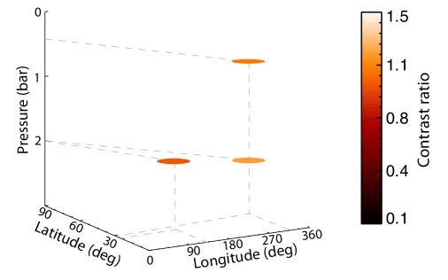
Figure 18: Jupiter’s model 3D structure based on our HST observations. From the observational light curves, Aeolus retrieves a number of spots per wavelength/pressure level. Using contribution functions we define the pressure level from which most of the radiation comes from, and create a 3D map of the jovian atmosphere.

In this paper we presented Aeolus, a Markov–Chain Monte Carlo code that maps the (2D) top–of–the–atmosphere (TOA) structure of brown dwarf and other directly detected ultra cool atmospheres, at a given observational wavelength. Aeolus combines a Metropolis-Hastings algorithm with a Gibbs sampler and assumes that all heterogeneities at the TOA appear in the form of elliptical spots (Cho & Polvani 1996; Cho et al. 2008). Aeolus finds the number of spots needed to fit the observed light curve, and for each spot its size, contrast ratio to the background and location (latitude and longitude) on the disk.

We validated Aeolus on the Jupiter dataset. Aeolus retrieved accurately the major features observed in the Jovian atmosphere. Aeolus, similarly to all flux–mapping techniques, cannot retrieve rotationally symmetric features (zones and belts of Jupiter) and suffers from latitudinal degeneracies (see e.g. Apai et al. 2013). The latter is the reason why Aeolus did not retrieve Oval BA (visible in the U–band), but found a slightly shifted latitude and larger size for the Great Red Spot (GRS). In the U–band Aeolus retrieved the biggest, non–rotationally–symmetric feature of the jovian disk (in the U–band), the GRS. In the R–band Aeolus retrieved the GRS and the largest 5 $\mu$m hot spot visible at the TOA. In both bands, smaller features such as high altitude NH₃ ice clouds, or smaller 5 $\mu$m hot spots were not retrieved. If we take into account that the Oval BA is large enough to influence the retrieved location and size of the GRS, then, the smallest feature retrieved by Aeolus in our HST Jupiter dataset has a longitudinal extent of $\sim$11^∘. Aeolus is, to our knowledge, the first mapping code validated on actual observations of a giant planet over a full rotational period.

Given the unprecedented high SNR (relative photometric per independent sample: $\sim$30,000) of these observations for the field of exoplanets and brown dwarfs, these results put constraints on the maximum size of TOA features we can map in the future using, for example, the James Webb Space Telescope (JWST). For example, modeling SIMP0136 spectrum as a black body (T_eff=1100K), normalized so that M${}_{\mathrm{J}}=$14.5 (Artigau et al. 2006; Apai et al. 2013) and assume we observe it with NIRCAM’s F200W with a 12$\mathrm{s}$ exposure (resolution of 0.5^∘ of rotation for SIMP0136) we reach a SNR$\sim$4,160 (source: JWST prototype ETC, version P1.6). Considering that JWST will provide a finer cadence than HST can, the combined information content over a complete rotation on a high–amplitude variable brown dwarf will be comparable with our current HST dataset on Jupiter. This suggests that mapping with an overall quality similar to that presented here may be possible for the most ideal brown dwarfs. Assuming a contrast range in the atmospheric features that is similar to that observed in Jupiter in the visible, rotational maps could identify features $\sim$11^∘ or larger, similar to the Oval BA in our study. (Kostov & Apai 2013) argues that with high–contrast observations JWST will also be able to carry out analogous observations on directly imaged exoplanets.

We explored our Jupiter observations for the possibility that our temporal (i.e., rotational, or spatial) resolution affects the minimum size of the mapped features. In particular, we explored the possibility that the largest time gaps in our observations (corresponding to rotational “jumps” of 32.5^∘ to 45.5^∘ and are due to Earth occultations of the target (Jupiter) with HST’s orbit) result in some of the features to not be followed throughout their rotation across the visible and illuminated disk, and to a lack of data during their appearance from, and/or disappearance to the dark side. Lack of ingress/egress data could influence the detectability of features, since the features’ properties may not be well–constrained. We found that largest hot spot (that we detect) undergoes a similar “jump” of 32.5^∘ to the dark side, implying that this should not be an important effect.

We then applied Aeolus to two brown dwarfs in the L/T transition, 2M2139 and SIMP0136. Apai et al. (2013) obtained HST observations of these brown dwarfs and mapped them using principal component analysis (PCA) and the mapping package Stratos. We compared Aeolus results against Stratos and Fourier mapping results. We found that, within the error bars, Aeolus and Stratos agree on the amount and coverage on the TOA of 2M2139 and SIMP0136, while Fourier mapping hints to larger longitudinal coverage.

A major difference between the Aeolus and Stratos+PCA results is that in the case of SIMP0136, Aeolus retrieved a mix of brighter and darker than the background TOA spots, while Stratos+PCA retrieved only one kind (brighter or darker) of spots. Aeolus fits the properties of the spots on the TOA freely, and independently of each other, without any prior assumptions, while Stratos uses PCA analysis to identify the smallest set of independent spectra (i.e., amount of different components/ surface contrast ratios), over the mean spectrum, that are needed to reproduce 96% of the observed spectral variations. Apai et al. (2013) using PCA found that only one spot–component is necessary to fit the observed variations of 2M2139 and SIMP0136, arguing that all spots are similar in nature (see Apai et al. 2013). In contrast, Aeolus found that the best-fit spots are composed of three (2M2139) or, potentially, two different surfaces (SIMP0136, taking into account the error bars). Apai et al. (2013) using Stratos found that there is a degeneracy between best-fit spot brightness and limb–darkening parameters and/or inclination of the brown dwarf. Given that in Aeolus these parameters are fixed, the differences between the maps can be due to a wrong assumption for the inclination (we assumed $0^{\circ}$) or limb–darkening (we used $c\sim$0.5). In the future, we will upgrade Aeolus to fit inclination and limb–darkening as free parameters.

For a direct comparison with Stratos, we ran a test case where we forced the contrast ratio of the spots to the background TOA to be the same for all spots. We kept the contrast ratio a factor of three brighter than the background TOA to match the Apai et al. (2013) results. Our code retrieved 3 spots (BIC 52) covering 21.4$\pm$9.6% of the top–of–the–atmosphere, in agreement with Stratos results. The BIC for this solution is comparable to the best–fit model, making it an equally acceptable solution for Aeolus. In the future, a synergy of Aeolus with PCA can be used to control the validity of the best-fit models.

An interesting result is that, in agreement with the complexity of the light curves, both Aeolus and Stratos find that no one or two spot models can interpret the observed light curves accurately. This implies a complex TOA structure for both 2M2139 and SIMP0136. A similar, or more complex TOA structure was inferred for Luhman 16B (Crossfield et al. 2014), and is also implied by the complex light curve shapes observed in other brown dwarfs (see, e.g., Metchev et al. 2015). This hints to complex dynamics in the atmospheres of brown dwarfs, which are predicted by models of atmospheric circulation (Showman & Kaspi 2013; Zhang & Showman 2014).

As a demonstration of the potential for constraining atmospheric dynamics from rotational maps we briefly explore the possibility of constraining wind speeds from the maximum sizes of the features mapped, following a Rhines–length–based argument laid out in Apai et al. (2013), and also adopted in Burgasser et al. (2014). Our Aeolus’ SIMP0136 and 2M2139 maps show features that are, on average, larger (in longitude/latitude) than the largest Jupiter feature. If we accept that our maps are accurate, and the retrieved spots uniform, this would imply a higher wind speed in the atmosphere of these brown dwarfs than in Jupiter’s (assuming that the maximum spot size is set by the atmospheric jet widths). For example, using as the larger spot of Jupiter the GRS with s${}_{1}\sim$17^∘ and for 2M2139 s${}_{2}\sim$39^∘, Jupiter’s period P${}_{1}\sim$10 hrs and 2M2139’s period P${}_{1}\sim$7.61 hrs and the equatorial jet wind speed on Jupiter U${}_{1}\sim$100 m/s, one can show that the wind speed on 2M2139 (assuming that the radius of 2M2139 is equal to Jupiter’s radius) is $\sim$690 m/s. This speed is between the wind speeds of our Solar System giant planets [e.g., 100 m/s for Jupiter, 500 m/s for Neptune de Pater & Lissauer (2010)] and highly irradiated exojupiters where wind speeds can reach a couple thousands of km/s (e.g., Snellen et al. 2010; Colón et al. 2012). Radigan et al. (2012) suggest a wind speed of 45 m/s for 2M2139, even though they caution that their estimate may be offset and longer observation would be necessary to determine the actual wind speeds. For the slightly later T dwarf SIMP0136, Showman & Kaspi (2013) using Artigau et al. (2009) input, find a wind speed of 300 m/s to 500 m/s. If these values are verified, they would suggest our largest mapped spots are “blends” of smaller spots, in a comparable way to Aeolus’ “blend” of Oval BA and the GRS.

An interesting result that emerged from the few brown dwarfs with high–quality simultaneous multi–wavelength observations is that light curves probing different pressure levels do not always line up with each other. Specifically, five light curves in the late–T brown dwarf 2M2228 Buenzli et al. (2012) observed between 1.1 and 5 $\mu$m showed a pressure–dependent phase lag. This was interpreted as evidence for large–scale longitudinal–vertical organization in the atmosphere Buenzli et al. (2012). Similar possible phase shift was reported in the L/T transition dwarf binary Luhman 16AB Biller et al. (2013). In contrast, the two L/T transition objects 2M2139 and SIMP0136 showed no phase shifts in the 1.1–1.7 $\mu$m wavelength range, suggesting vertically identical surface brightness distribution (Apai et al. 2013). Thus, the presence or absence of pressure–dependent phase shifts provides powerful constraints on the longitudal–vertical structure of the atmospheres.

Analogously, the different wavelength observations of the jovian atmosphere presented in our paper also probe different pressure levels. The differently shaped light curves reveal different surface brightness distributions (Fig. 18 and Sect. 3.2). We note that if these light curves were observed with a SNR too low to allow distinguishing the differences in the light curve shape, the different peak times in the different light curves could be interpreted as phase shifts, even though they represent two uncorrelated structures.

We propose that to ensure that uncorrelated light curves are not misinterpreted as phase shifts a crucial consideration should be the uncertainties along both the pressure and the phase shifts axes. The presence or absence of vertically organized atmospheric layers could be tested by comparing the goodness of a single trend versus multiple uncorrelated trends in the pressure–phase shift space, considering the error bars.

In this paper we presented two–dimensional maps of Jupiter and two brown dwarfs: 2M2139 and SIMP0136. Aeolus though, can also produce three–dimensional maps of ultracool atmospheres. When the latter are observed at multiple wavelengths, Aeolus can produce two–dimensional maps of the atmosphere per observational wavelength. Using information from a target–appropriate contribution function, we can identify the pressure level where most of the radiation emerges from [at that wavelength; see, e.g., Buenzli et al. (2012)] and stack–up the two–dimensional maps. For example, in the case of Jupiter’s HST observations, contribution functions suggest that the R–band originates around $2$ bars and the U–band around $400$ mbar. With this information and the Aeolus retrieved maps, we can compose a “3D” map of the modeled jovian atmosphere as in Fig. 18. Studying the 3D structure of ultracool atmospheres and its variability over time is an important step towards understanding their dynamics. Long–scale atmospheric dynamical effects like cells and vortices, for example, will cause spots to move in 3D following the dynamical structure. Using multiple–epoch, multi–wavelength observations and Aeolus we can map the 3D structure of our targets over large periods and follow the 3D motions of structures in the atmospheres. These maps can then provide feedback to dynamical models, helping to study and understand dynamics governing ultracool atmospheres.

Aeolus is a validated mapping code that can be used to map brown dwarf and directly imaged giant exoplanet atmospheres currently, and imaged terrestrial exoplanets in the future. For the latter, an adaptation of Aeolus that takes into account surface (non–elliptical) structures would be necessary. Ideally, the updated version of Aeolus would then be validated on a “ground truth” dataset of Earth and/or Venus disk–integrated, multi–wavelength observations.

Aeolus was, in part, developed to interpret observations from the Extrasolar Storms program (PI: Apai). Extrasolar Storms obtained multi–epoch HST and Spitzer observations of six brown dwarfs, to characterize cloud evolution and dynamics of brown dwarf atmospheres over multiple rotational periods. Extrasolar Storms observed six targets, in eight separate visits from Spitzer’s IRAC channels 1 and 2, and two visits from HST WFC3 IR channel (G141). HST visits were coordinated with the Spitzer observations, so that for two visits we acquired multi–wavelength observations. We, currently, apply Aeolus on the full Extrasolar Storms sample and will publish our results in a follow–up paper.

6 Conclusions

We presented Aeolus, a Markov–Chain Monte Carlo code that maps the two–dimensional top–of–the–atmosphere structure of brown dwarf and other directly detected ultra cool atmospheres, at a given observational wavelength. We validated Aeolus on a unique spatially and temporally resolved imaging data set of the full disk of Jupiter in two spectral bands. This data set provides a“truth test” to validate mapping of ultracool atmospheres by Aeolus and any other mapping methods/ tools. The dataset will be publicly available via ADS/VIZIR. Aeolus is the first mapping code validated on actual observations of a giant planet over a full rotational period.

We noted that if our Jupiter light curves were observed with a signal–to–noise–ratio too low to allow distinguishing the differences in the light curve shape, the different peak times in the different light curves could be interpreted as phase shifts, analogous to the ones seen in 2M2228, even though they represent two uncorrelated structures. To ensure that uncorrelated light curves are not misinterpreted as phase shifts we need better constrains of the uncertainties along both the pressure and the phase shifts axes.

Finally, we applied Aeolus to 2M2139 and SIMP0136. Aeolus found three spots at the top–of–the–atmosphere of these two brown dwarfs, with a coverage of 21%$\pm$3% and 20.3%$\pm$1.5% respectively, in agreement with previous mapping efforts. Constraining wind speeds from the maximum sizes of the features in Aeolus’ maps we retrieved a wind speed of $\sim$690 m/s for 2M2139. Observations of 2M2139 and SIMP0136 suggest lower wind speeds, up to 500 m/s, which, if confirmed, imply that Aeolus’ largest features mapped are blends of smaller spots.

References

- Apai et al. (2013) Apai, D., Radigan, J., Buenzli, E., Burrows, A., Reid, I. N., & Jayawardhana, R. 2013, ApJ, 768, 121
- Artigau et al. (2009) Artigau, É., Bouchard, S., Doyon, R., & Lafrenière, D. 2009, ApJ, 701, 1534
- Artigau et al. (2006) Artigau, É., Doyon, R., Lafrenière, D., Nadeau, D., Robert, J., & Albert, L. 2006, ApJ, 651, L57
- Atreya et al. (2005) Atreya, S. K., Wong, A. S., Baines, K. H., Wong, M. H., & Owen, T. C. 2005, Planet. Space Sci., 53, 498
- Bagenal et al. (2004) Bagenal, F., Dowling, T. E., & McKinnon, W. B. 2004, Jupiter : the planet, satellites and magnetosphere (Cambridge University Press)
- Bean et al. (2010) Bean, J. L., Miller-Ricci Kempton, E., & Homeier, D. 2010, Nature, 468, 669
- Biller et al. (2013) Biller, B. A., Crossfield, I. J. M., Mancini, L., Ciceri, S., Southworth, J., Kopytova, T. G., Bonnefoy, M., Deacon, N. R., Schlieder, J. E., Buenzli, E., Brandner, W., Allard, F., Homeier, D., Freytag, B., Bailer-Jones, C. A. L., Greiner, J., Henning, T., & Goldman, B. 2013, ApJ, 778, L10
- Buenzli et al. (2012) Buenzli, E., Apai, D., Morley, C. V., Flateau, D., Showman, A. P., Burrows, A., Marley, M. S., Lewis, N. K., & Reid, I. N. 2012, ApJ, 760, L31
- Buenzli et al. (2015) Buenzli, E., Saumon, D., Marley, M. S., Apai, D., Radigan, J., Bedin, L. R., Reid, I. N., & Morley, C. V. 2015, ApJ, 798, 127
- Burgasser et al. (2010) Burgasser, A. J., Cruz, K. L., Cushing, M., Gelino, C. R., Looper, D. L., Faherty, J. K., Kirkpatrick, J. D., & Reid, I. N. 2010, ApJ, 710, 1142
- Burgasser et al. (2006) Burgasser, A. J., Geballe, T. R., Leggett, S. K., Kirkpatrick, J. D., & Golimowski, D. A. 2006, ApJ, 637, 1067
- Burgasser et al. (2014) Burgasser, A. J., Gillon, M., Faherty, J. K., Radigan, J., Triaud, A. H. M. J., Plavchan, P., Street, R., Jehin, E., Delrez, L., & Opitom, C. 2014, ApJ, 785, 48
- Burrows et al. (2006) Burrows, A., Sudarsky, D., & Hubeny, I. 2006, ApJ, 640, 1063
- Chib & Greenberg (1995) Chib, S. & Greenberg, E. 1995, The American Statistician, 49, No 4
- Cho et al. (2008) Cho, J. Y.-K., Menou, K., Hansen, B. M. S., & Seager, S. 2008, ApJ, 675, 817
- Cho & Polvani (1996) Cho, J. Y. K. & Polvani, L. M. 1996, Phys. Fluids, 8, 1531
- Choi et al. (2013) Choi, D. S., Showman, A. P., Vasavada, A. R., & Simon-Miller, A. A. 2013, Icarus, 223, 832
- Colón et al. (2012) Colón, K. D., Ford, E. B., Redfield, S., Fortney, J. J., Shabram, M., Deeg, H. J., & Mahadevan, S. 2012, MNRAS, 419, 2233
- Cowan & Agol (2008) Cowan, N. B. & Agol, E. 2008, ApJ, 678, L129
- Cowan et al. (2009) Cowan, N. B., Agol, E., Meadows, V. S., Robinson, T., Livengood, T. A., Deming, D., Lisse, C. M., A’Hearn, M. F., Wellnitz, D. D., Seager, S., Charbonneau, D., & EPOXI Team. 2009, ApJ, 700, 915
- Cowan et al. (2013) Cowan, N. B., Fuentes, P. A., & Haggard, H. M. 2013, MNRAS, 434, 2465
- Crossfield et al. (2014) Crossfield, I. J. M., Biller, B., Schlieder, J. E., Deacon, N. R., Bonnefoy, M., Homeier, D., Allard, F., Buenzli, E., Henning, T., Brandner, W., Goldman, B., & Kopytova, T. 2014, Nature, 505, 654
- de Pater & Lissauer (2010) de Pater, I. & Lissauer, J. J. 2010, Planetary Sciences (Cambridge University Press)
- de Wit et al. (2012) de Wit, J., Gillon, M., Demory, B.-O., & Seager, S. 2012, A&A, 548, A128
- Demory et al. (2013) Demory, B.-O., de Wit, J., Lewis, N., Fortney, J., Zsom, A., Seager, S., Knutson, H., Heng, K., Madhusudhan, N., Gillon, M., Barclay, T., Desert, J.-M., Parmentier, V., & Cowan, N. B. 2013, ApJ, 776, L25
- Ford (2005) Ford, E. B. 2005, Astronomical Journal, 129, 1706
- Friedson et al. (2002) Friedson, A. J., Wong, A.-S., & Yung, Y. L. 2002, Icarus, 158, 389
- Gelman & Rubin (1992) Gelman, A. & Rubin, D. B. 1992, Stat. Sci., 7, 457
- Goldman et al. (2008) Goldman, B., Bouy, H., Zapatero Osorio, M. R., Stumpf, M. B., Brandner, W., & Henning, T. 2008, A&A, 490, 763
- Ingersoll et al. (2004) Ingersoll, A. P., Dowling, T. E., Gierasch, P. J., Orton, G. S., Read, P. L., Sánchez-Lavega, A., Showman, A. P., Simon-Miller, A. A., & Vasavada, A. R. Dynamics of Jupiter’s atmosphere, ed. F. Bagenal, T. E. Dowling, & W. B. McKinnon (Cambridge University Press), 105–128
- Irwin (2003) Irwin, P. G. J. 2003, Giant planets of our solar system : atmospheres compositions, and structure (Springer-Verlag Berlin Heidelberg)
- Irwin et al. (2011) Irwin, P. G. J., Teanby, N. A., Davis, G. R., Fletcher, L. N., Orton, G. S., Tice, D., Hurley, J., & Calcutt, S. B. 2011, Icarus, 216, 141
- Karalidi et al. (2013) Karalidi, T., Stam, D. M., & Guirado, D. 2013, A&A, 555, A127
- Kipping (2012) Kipping, D. M. 2012, MNRAS, 427, 2487
- Knutson et al. (2007) Knutson, H. A., Charbonneau, D., Allen, L. E., Fortney, J. J., Agol, E., Cowan, N. B., Showman, A. P., Cooper, C. S., & Megeath, S. T. 2007, Nature, 447, 183
- Knutson et al. (2014) Knutson, H. A., Dragomir, D., Kreidberg, L., Kempton, E. M.-R., McCullough, P. R., Fortney, J. J., Bean, J. L., Gillon, M., Homeier, D., & Howard, A. W. 2014, ArXiv e-prints
- Kostov & Apai (2013) Kostov, V. & Apai, D. 2013, ApJ, 762, 47
- Kreidberg et al. (2014) Kreidberg, L., Bean, J. L., Désert, J.-M., Benneke, B., Deming, D., Stevenson, K. B., Seager, S., Berta-Thompson, Z., Seifahrt, A., & Homeier, D. 2014, Nature, 505, 69
- Luhman (2013) Luhman, K. L. 2013, ApJ, 767, L1
- Luhman et al. (2014) Luhman, K. L., Morley, C. V., Burgasser, A. J., Esplin, T. L., & Bochanski, J. J. 2014, ApJ, 794, 16
- Marley et al. (2013) Marley, M. S., Ackerman, A. S., Cuzzi, J. N., & Kitzmann, D. Clouds and Hazes in Exoplanet Atmospheres, ed. S. J. Mackwell, A. A. Simon-Miller, J. W. Harder, & M. A. Bullock (The University of Arizona Press), 367–391
- Marley et al. (2010) Marley, M. S., Saumon, D., & Goldblatt, C. 2010, ApJ, 723, L117
- Marley et al. (2002) Marley, M. S., Seager, S., Saumon, D., Lodders, K., Ackerman, A. S., Freedman, R. S., & Fan, X. 2002, ApJ, 568, 335
- Metchev et al. (2015) Metchev, S. A., Heinze, A., Apai, D., Flateau, D., Radigan, J., Burgasser, A., Marley, M. S., Artigau, É., Plavchan, P., & Goldman, B. 2015, ApJ, 799, 154
- Metchev et al. (2013) Metchev, S., Apai, D., Radigan, J., Artigau, É., Heinze, A., Helling, C., Homeier, D., Littlefair, S., Morley, C., Skemer, A., & Stark, C. 2013, Astronomische Nachrichten, 334, 40
- Milone & Wilson (2014) Milone, E. F. & Wilson, W. J. F. 2014, Solar System Astrophysics: Planetary Atmospheres and the Outer Solar System (Springer-Verlag New York)
- Morley et al. (2014a) Morley, C. V., Marley, M. S., Fortney, J. J., & Lupu, R. 2014a, ApJ, 789, L14
- Morley et al. (2014b) Morley, C. V., Marley, M. S., Fortney, J. J., Lupu, R., Saumon, D., Greene, T., & Lodders, K. 2014b, ApJ, 787, 78
- Ortiz et al. (1998) Ortiz, J. L., Orton, G. S., Friedson, A. J., Stewart, S. T., Fisher, B. M., & Spencer, J. R. 1998, J. Geophys. Res., 103, 23051
- Pasachoff (2012) Pasachoff, J. M. 2012, in American Astronomical Society Meeting Abstracts, Vol. 220, American Astronomical Society Meeting Abstracts #220, #127.01
- Pasachoff et al. (2013a) Pasachoff, J. M., Schneider, G., Babcock, B. A., Lu, M., Edelman, E., Reardon, K., Widemann, T., Tanga, P., Dantowitz, R., Silverstone, M. D., Ehrenreich, D., Vidal-Madjar, A., Nicholson, P. D., Willson, R. C., Kopp, G. A., Yurchyshyn, V. B., Sterling, A. C., Scherrer, P. H., Schou, J., Golub, L., McCauley, P., & Reeves, K. 2013a, in American Astronomical Society Meeting Abstracts, Vol. 221, American Astronomical Society Meeting Abstracts #221, #315.06
- Pasachoff et al. (2013b) Pasachoff, J. M., Schneider, G., Babcock, B. A., Lu, M., Penn, M. J., Jaeggli, S. A., Galayda, E., Reardon, K. P., Widemann, T., Tanga, P., Ehrenreich, D., Vidal-Madjar, A., Nicholson, P. D., & Dantowitz, R. 2013b, in American Astronomical Society Meeting Abstracts, Vol. 222, American Astronomical Society Meeting Abstracts, #217.01
- Pont et al. (2008) Pont, F., Knutson, H., Gilliland, R. L., Moutou, C., & Charbonneau, D. 2008, Monthly Notices of the Royal Astronomical Society, 385, 109
- Pryor & Hord (1991) Pryor, W. R. & Hord, C. W. 1991, Icarus, 91, 161
- Radigan et al. (2012) Radigan, J., Jayawardhana, R., Lafrenière, D., Artigau, É., Marley, M., & Saumon, D. 2012, ApJ, 750, 105
- Schwarz (1978) Schwarz, G. 1978, Annals of Statistics, 6, 461
- Shetty & Marcus (2010) Shetty, S. & Marcus, P. S. 2010, Icarus, 210, 182
- Showman & Kaspi (2013) Showman, A. P. & Kaspi, Y. 2013, ApJ, 776, 85
- Simon-Miller et al. (2001) Simon-Miller, A. A., Banfield, D., & Gierasch, P. J. 2001, Icarus, 154, 459
- Simon-Miller et al. (2002) Simon-Miller, A. A., Gierasch, P. J., Beebe, R. F., Conrath, B., Flasar, F. M., Achterberg, R. K., & the Cassini CIRS Team. 2002, Icarus, 158, 249
- Sing et al. (2013) Sing, D. K., Lecavelier des Etangs, A., Fortney, J. J., Burrows, A. S., Pont, F., Wakeford, H. R., Ballester, G. E., Nikolov, N., Henry, G. W., Aigrain, S., Deming, D., Evans, T. M., Gibson, N. P., Huitson, C. M., Knutson, H., Showman, A. P., Vidal-Madjar, A., Wilson, P. A., Williamson, M. H., & Zahnle, K. 2013, Monthly Notices of the Royal Astronomical Society, 436, 2956
- Smith et al. (1981) Smith, B. A., Soderblom, L., Beebe, R. F., Boyce, J. M., Briggs, G., Bunker, A., Collins, S. A., Hansen, C., Johnson, T. V., Mitchell, J. L., Terrile, R. J., Carr, M. H., Cook, A. F., Cuzzi, J. N., Pollack, J. B., Danielson, G. E., Ingersoll, A. P., Davies, M. E., Hunt, G. E., Masursky, H., Shoemaker, E. M., Morrison, D., Owen, T., Sagan, C., Veverka, J., Strom, R., & Suomi, V. E. 1981, Science, 212, 163
- Snellen et al. (2010) Snellen, I. A. G., de Kok, R. J., de Mooij, E. J. W., & Albrecht, S. 2010, Nature, 465, 1049
- Snellen et al. (2009) Snellen, I. A. G., de Mooij, E. J. W., & Albrecht, S. 2009, Nature, 459, 543
- Sromovsky et al. (2002) Sromovsky, L. A., Fry, P. M., & Baines, K. H. 2002, Icarus, 156, 16
- Sromovsky et al. (2012) Sromovsky, L. A., Hammel, H. B., de Pater, I., Fry, P. M., Rages, K. A., Showalter, M. R., Merline, W. J., Tamblyn, P., Neyman, C., Margot, J.-L., Fang, J., Colas, F., Dauvergne, J.-L., Gómez-Forrellad, J. M., Hueso, R., Sánchez-Lavega, A., & Stallard, T. 2012, Icarus, 220, 6
- Teifel (1976) Teifel, V. G. 1976, Soviet Ast., 19, 373
- Tierney (1994) Tierney, L. 1994, The Annals of Statistics, 22(4), 1701-1762
- Trigo-Rodriguez et al. (2000) Trigo-Rodriguez, J. M., Sánchez-Lavega, A., Gómez, J. M., Lecacheux, J., Colas, F., & Miyazaki, I. 2000, Planet. Space Sci., 48, 331
- Ivezić et al. (2014) Ivezić, Ż., Connolly, A., VanderPlas, J., & Gray, A. 2014, Statistics, Data Mining, and Machine Learning in Astronomy (Princeton University Press)
- Vasavada & Showman (2005) Vasavada, A. R. & Showman, A. P. 2005, Reports on Progress in Physics, 68, 1935
- Vincent et al. (2000) Vincent, M. B., Clarke, J. T., Ballester, G. E., Harris, W. M., West, R. A., Trauger, J. T., Evans, R. W., Stapelfeldt, K. R., Crisp, D., Burrows, C. J., Gallagher, J. S., Griffiths, R. E., Jeff Hester, J., Hoessel, J. G., Holtzman, J. A., Mould, J. R., Scowen, P. A., Watson, A. M., & Westphal, J. A. 2000, Icarus, 143, 189
- West et al. (2009) West, R. A., Baines, K. H., Karkoschka, E., & Sánchez-Lavega, A. Clouds and Aerosols in Saturn’s Atmosphere, ed. M. K. Dougherty, L. W. Esposito, & S. M. Krimigis (Springer Netherlands), 161
- West & Smith (1991) West, R. A. & Smith, P. H. 1991, Icarus, 90, 330
- West et al. (1986) West, R. A., Strobel, D. F., & Tomasko, M. G. 1986, Icarus, 65, 161
- Wong et al. (2011) Wong, M. H., de Pater, I., Asay-Davis, X., Marcus, P. S., & Go, C. Y. 2011, Icarus, 215, 211
- Yang et al. (2015) Yang, H., Apai, D., Marley, M. S., Saumon, D., Morley, C. V., Buenzli, E., Artigau, É., Radigan, J., Metchev, S., Burgasser, A. J., Mohanty, S., Lowrance, P. J., Showman, A. P., Karalidi, T., Flateau, D., & Heinze, A. N. 2015, ApJ, 798, L13
- Zhang & Showman (2014) Zhang, X. & Showman, A. P. 2014, ApJ, 788, L6