Contrast estimation for parametric stationary determinantal point processes

Abstract

We study minimum contrast estimation for parametric stationary determinantal point processes. These processes form a useful class of models for repulsive (or regular, or inhibitive) point patterns and are already applied in numerous statistical applications. Our main focus is on minimum contrast methods based on the Ripley’s $K$-function or on the pair correlation function. Strong consistency and asymptotic normality of theses procedures are proved under general conditions that only concern the existence of the process and its regularity with respect to the parameters. A key ingredient of the proofs is the recently established Brillinger mixing property of stationary determinantal point processes. This work may be viewed as a complement to the study of Y. Guan and M. Sherman who establish the same kind of asymptotic properties for a large class of Cox processes, which in turn are models for clustering (or aggregation).

Ripley’s $K$ function, pair correlation function, Brillinger mixing, central limit theorem.

1 Introduction

Determinantal point processes (DPPs) are models for repulsive (or regular, or inhibitive) point processes data. They have been introduced by O. Macchi in [21] to model the position of fermions, which are particles that repel each others. Their probabilistic aspects have been studied thoroughly, in particular in [28], [27] and [13]. Recently, DPPs have been studied and applied from a statistical perspective. A description of their main statistical aspects is conducted in [19] and they actually turn out to be a well-adapted statistical model in domains as statistical learning [16], telecommunications [8, 22], biology and ecology (see the examples in [19] and [18]).

A DPP is defined through a kernel $C$, basically a covariance function. Assuming a parametric form for $C$, several estimation procedures are considered in [19], specifically the maximum likelihood method and minimum contrast procedures based on the Ripley’s $K$ function or the pair correlation $g$. These methods are implemented in the spatstat library [1, 2] of R [25]. From the simulation study conducted in [19] and [18], see also Section 2.2, the maximum likelihood procedure seems to be the best method in terms of quadratic loss. However, the expression of the likelihood relies in theory on a spectral representation of $C$, which is rarely known in practice, and some Fourier approximations are introduced in [19]. The likelihood also involves the determinant of a $n\times n$ matrix, where $n$ is the number of observed points, which is prohibitively time consuming to compute when $n$ is large. In contrast, the estimation procedures based on $K$ or $g$ do not require the knowledge of any spectral representation of $C$ and are faster to compute in presence of large datasets, which explain their importance in practice.

From a theoretical point of view, neither the likelihood method nor the minimum contrast methods for DPPs have been studied thoroughly, even in assuming that a spectral method for $C$ is known. In this work, we focus on parametric stationary DPPs and we prove the strong consistency and the asymptotic normality of the minimum contrast estimators based on $K$ and $g$. These questions are in connection with the general investigation of Y. Guan and M. Sherman [10], who study the asymptotic properties of the latter estimators for stationary point processes. However the setting in [10] has a clear view to Cox processes and the assumptions involve both $\alpha$-mixing and Brillinger mixing conditions, which are indeed satisfied for a large class of Cox processes. Unfortunately these results do no apply straightforwardly to DPPs. We consider instead more general versions of the asymptotic theorems in [10] and we prove that they apply nicely to DPPs. Our main ingredient then becomes the Brillinger mixing property of stationary DPPs, recently proved in [4], and we do not need any $\alpha$-mixing condition. Our asymptotic results finally gather a very large class of stationary DPPs, where the main assumptions are quite standard and only concern the regularity of the kernel $C$ with respect to the parameters. As an extension to the results in [10], it is worth mentioning the study of [32] dealing with constrast estimation for some inhomogeneous spatial point processes, still under a crucial $\alpha$-mixing condition. We do not address this generalization for DPPs in the present work.

The remainder of this paper is organized as follows. In Section 2, we recall the definition of stationary DPPs, some of their basic properties and we discuss parametric estimation of DPPs. Our main results are presented in Section 3, namely the asymptotic properties of the minimum contrast estimators of a DPP based on the $K$ or the $g$ function. Section 4 gathers the proofs of our main results. In the appendix, we finally present our general asymptotic result for minimum contrast estimators and some auxiliary materials.

2 Stationary DPPs and parametric estimation

2.1 Stationary DPPs

We refer to [6, 7] for a general presentation on point processes. Let $\mathbf{X}$ be a simple point process on $\mathbb{R}^{d}$. For a bounded set $D\subset\mathbb{R}^{d}$, denote by $\mathbf{X}(D)$ the number of points of $\mathbf{X}$ in $D$ and let $E$ be the expectation over the distribution of $\mathbf{X}$. If there exists a function $\rho^{(k)}:(\mathbb{R}^{d})^{k}\to\mathbb{R}^{+}$, for $k\geq 1$, such that for any family of mutually disjoint subsets $D_{1},\dots,D_{k}$ in $\mathbb{R}^{d}$

$$E\prod_{i=1}^{k}\mathbf{X}(D_{i})=\int_{D_{1}}\dots\int_{D_{k}}\rho^{(k)}(x_{1},\dots,x_{k})dx_{1}\dots dx_{k},$$

then this function is called the joint intensity of order $k$ of $\mathbf{X}$. If $\mathbf{X}$ is stationary, $\rho^{(k)}(x_{1},\dots,x_{k})=\rho^{(k)}(0,x_{2}-x_{1},\dots,x_{k}-x_{1})$ and in particular $\rho^{(1)}=\rho$ is a constant. From its definition, the joint intensity of order $k$ is unique up to a Lebesgue nullset. Henceforth, for ease of presentation, we ignore nullsets. In particular we will say that a function is continuous whenever there exists a continuous version of it.

Determinantal point processes (DPPs) are defined through their joint intensities. We refer to the survey by Hough et al. [13] for a general presentation including the non-stationary case and the extension to complex-valued kernels. We focus in this work on stationary DPPs and so we restrict the definition to this subclass. We also consider for simplicity real-valued kernels.

Definition 2.1.

Let $C:\mathbb{R}^{d}\rightarrow\mathbb{R}$ be a function. A point process $\mathbf{X}$ on $\mathbb{R}^{d}$ is a stationary DPP with kernel $C$, in short $\mathbf{X}\sim DPP(C)$, if for all $k\geq 1$ its joint intensity of order $k$ exists and satisfies the relation

$$\rho^{(k)}(x_{1},\ldots x_{k})=\det[C](x_{1},\dots,x_{k})$$

for every $(x_{1},\dots,x_{k})\in\mathbb{R}^{dk}$, where $[C](x_{1},\dots,x_{k})$ denotes the matrix with entries $C(x_{i}-x_{j})$, $1\leq i,j\leq k$.

Conditions on $C$ ensuring the existence of $DPP(C)$ are recalled in the next proposition. We define the Fourier transform of a function $h\in L^{1}(\mathbb{R}^{d})$ as

$$\mathcal{F}(h)(t)=\int_{\mathbb{R}^{d}}h(x)e^{2i\pi x\cdot t}dx,\quad\forall t\in\mathbb{R}^{d}$$

and we consider its extension to $L^{2}(\mathbb{R}^{d})$ by Plancherel’s theorem, see [30].

Condition $\mathcal{K}(\rho)$. A kernel $C$ is said to verify condition $\mathcal{K}(\rho)$ if $C$ is a symmetric continuous real-valued function in $L^{2}(\mathbb{R}^{d})$ with $C(0)=\rho$ and $0\leq\mathcal{F}(C)\leq 1$.

Proposition 2.2 ([28, 19]).

Assume $C$ satisfies $\mathcal{K}(\rho)$. Then $DPP(C)$ exists and is unique if and only if $0\leq\mathcal{F}(C)\leq 1$.

In short, $DPP(C)$ exists whenever $C$ is a continuous covariance function in $L^{2}(\mathbb{R}^{d})$ with $\mathcal{F}(C)\leq 1$. This makes easy the construction of parametric families of DPPs, simply considering parametric families of covariance functions where the condition $\mathcal{F}(C)\leq 1$ appears as a constraint on the parameters. Some examples are given in [19], [5] and in the next section.

By definition, all moments of a DPP are known, in particular the pair correlation (pcf) and the Ripley’s $K$-function can explicitly be expressed in terms of the kernel. For $C$ satisfying $\mathcal{K}(\rho)$, let $R(x)=C(x)/C(0)$ be the correlation function associated to $C$. The pcf, defined in the stationary case for all $x\in\mathbb{R}^{d}$ by $g(x)={\rho^{(2)}(0,x)}/{\rho^{2}}$, writes

$$g(x)=1-R^{2}(x).$$

The Ripley’s $K$-function is in turn given for all $t\geq 0$ by

$$K(t)=\int_{B(0,t)}g(x)dx=\int_{B(0,t)}(1-R^{2}(x))dx$$ (2.1)

where $B(0,t)$ is the Euclidean ball centred at $0$ with radius $t$. For later purposes, we denote by $c_{[k]}^{red}$ the density of the reduced factorial cumulant moment measures of order $k$ of $\mathbf{X}$. We refer to [4] for the definition and further details, where the following particular cases are derived. Assuming that the kernel $C$ of $\mathbf{X}$ satisfies $\mathcal{K}(\rho)$, we have for all $(u,v,w)\in\mathbb{R}^{3d}$

$$c^{red}_{[2]}(u)=-C^{2}(u),$$ (2.2)

$$c^{red}_{[3]}(u,v)=\ 2\ C(u)C(v)C(v-u),$$ (2.3)

$$c^{red}_{[4]}(u,v,w)=-2\big{[}C(u)C(v)C(u-w)C(v-w)+C(u)C(w)C(u-v)C(v-w)$$

$$\hskip 56.9055pt+C(v)C(w)C(u-v)C(u-w)\big{]}.$$ (2.4)

2.2 Parametric estimation of DPPs

We consider a parametric family of DPPs with kernel $C_{\rho,\theta}$ where $\rho=C_{\rho,\theta}(0)>0$ and $\theta$ belongs to a subset $\Theta_{\rho}$ of $\mathbb{R}^{p}$, for a given $p\geq 1$. To ensure the existence of $DPP(C_{\rho,\theta})$, we assume that for all $\rho>0$ and any $\theta\in\Theta_{\rho}$, the kernel $C_{\rho,\theta}$ verifies $\mathcal{K}(\rho)$, which explains the indexation of $\Theta_{\rho}$ by $\rho$. We assume further that for a given $\rho_{0}>0$ and $\theta_{0}$ in the interior of $\Theta_{\rho_{0}}$ (provided this interior is non-empty) we observe the point process $\mathbf{X}\sim DPP(C_{\rho_{0},\theta_{0}})$ on a bounded domain $D_{n}\subset\mathbb{R}^{d}$.

The standard estimator of the intensity $\rho_{0}$ is

$${\widehat{\rho}_{n}}=\frac{1}{|D_{n}|}\sum_{x\in\mathbf{X}}\mathbf{1}_{\{x\in D_{n}\}}$$ (2.5)

where $|D_{n}|$ denotes the Lebesgue volume of $D_{n}$. Since a stationary DPP is ergodic, see [28], this estimator is strongly consistent by the ergodic theorem, and it is asymptotically normal, cf [29] and [4]. In the following, we focus our attention on the estimation of $\theta_{0}$. As explained in [18], likelihood inference is in theory feasible if we know a spectral representation of $C_{\rho,\theta}$ on $D_{n}$. Unfortunately no spectral representations are known in the general case and some Fourier approximations are introduced in [18]. Another option is to consider minimum contrast estimators (MCE) as described below.

For $\rho>0$ and $\theta\in\Theta_{\rho}$, let $J(.,\theta)$ be a function from $\mathbb{R}^{d}$ into $\mathbb{R}^{+}$ which is a summary statistic of $DPP(C_{\rho,\theta})$ that does not depend on $\rho$. In the DPP’s case, the most important and natural examples are the $K$-function and the pcf $g$, that we study in detail in the following. Consider $\widehat{J}_{n}$ an estimator of $J$ from the observation of $\mathbf{X}$ on $D_{n}$. Further, let $c\in\mathbb{R}$, $c\neq 0$, be a parameter such that $\widehat{J}_{n}(t)^{c}$ and $J(t,\theta)^{c}$ are well defined for all $t\in\mathbb{R}$ and $\theta\in\Theta_{\rho_{0}}$. Finally, define for $0\leq{r_{min}}<{r_{max}}$, the discrepancy measure

$$U_{n}(\theta)=\int_{{r_{min}}}^{{r_{max}}}w(t)\left\{\widehat{J}_{n}(t)^{c}-J(t,\theta)^{c}\right\}^{2}dt$$ (2.6)

where $w$ is a smooth weight function. The MCE of $\theta_{0}$ is

$$\widehat{\theta}_{n}=\operatorname*{arg\,min}_{\theta\in\Theta_{\hat{\rho}_{n}}}U_{n}(\theta).$$ (2.7)

For example, let us consider the parametric family of DPPs with Gaussian kernels

$$C(x)=\rho e^{-\left|\frac{x}{\alpha}\right|^{2}},\quad x\in\mathbb{R}^{d},$$ (2.8)

where $|.|$ denote the Euclidean norm on $\mathbb{R}^{d}$, $\rho>0$ and $\alpha\leq 1/(\sqrt{\pi}\rho^{1/d})$, the latter constraint on the parameter space being a consequence of the existence condition $\mathcal{F}(C)\leq 1$ in $K(\rho)$. Some realizations are shown in Figure 1. For comparison, we have estimated the parameter $\alpha$ of this model with the MCE (2.7) when $J$ corresponds to $K$ or $g$, and with the maximum likelihood method (using the Fourier approximation of the spectral representation of $C$ introduced in [19]). The estimators of $K$ and $g$, in place of $\widehat{J}_{n}$ in (2.7), are standard and recalled in Sections 3.2-3.3, see also [23, Chapter 4]. For the tuning parameters, we followed the standard choice $w(t)=1$, $r_{\min}=0.01$, $r_{\max}$ as one quarter of the side length of the window and $c=0.5$ as recommended in [9] for repulsive point processes. This simulation study has been carried out with the functions implemented in the spatstat library. Table 1 reports the mean squared errors of the three mentioned methods over $500$ realisations of $DPP(C)$ with $\rho=100$ and $\alpha=0.01,\ 0.03,\ \frac{1}{10\sqrt{\pi}}$, observed on $[0,1]^{2}$, $[0,2]^{2}$ and $[0,3]^{2}$.

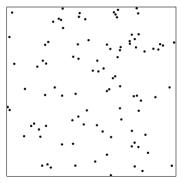
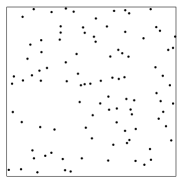
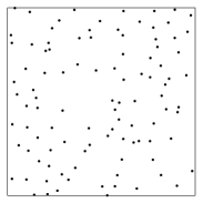
Figure 1: Realizations on $[0,1]^{2}$ of DPPs with kernel (2.8) where $\rho=100$ and from left to right $\alpha=0.01,\ 0.03,\ \frac{1}{10\sqrt{\pi}}$.

	$[0,1]^{2}$			$[0,2]^{2}$			$[0,3]^{2}$
	$K$	$g$	ML	$K$	$g$	ML	$K$	$g$	ML
$\alpha=0.01$	2.026	1.039	1.032	0.848	0.309	0.220	0.521	0.175	0.096
$\alpha=0.03$	1.214	0.706	0.786	0.419	0.248	0.175	0.231	0.180	0.084
$\alpha=1/(10\sqrt{\pi})$	0.356	0.588	0.225	0.113	0.258	0.061	0.051	0.176	0.022

Table 1: Mean squared errors of the MCE (2.7) when $J=K$, $J=g$, and the maximum likelihood method estimator (ML) as approximated in [19]. These values are estimated from 500 realizations of DPPs on $[0,1]^{2}$, $[0,2]^{2}$ and $[0,3]^{3}$ with kernel (2.8), $\rho=100$ and $\alpha=0.01,\ 0.03,\ \frac{1}{10\sqrt{\pi}}$. All entries are multiplied by $10^{4}$ to make the table more compact.

For all methods considered in Table 1, the estimators seem consistent and the precision, in the sense of the mean squared errors, increases with the size of the observation window. From these results, the maximum likelihood method seems to be the best method in terms of quadradic loss, which agrees with the observations made in [19]. However, MCEs, especially the one based on $g$, seem to perform reasonably well. Moreover, their computation is faster than the maximum likelihood method and do not rely on an approximated spectral representation of $C$. For instance, with a regular laptop, the estimation of $\alpha$ for 500 realizations on $[0,3]^{2}$ took about 30 minutes for the MCEs based on $K$ and $g$ against more than 7 hours by the maximum likelihood method. Finally, it seems that each estimator has an asymptotic Gaussian behaviour, as illustrated in Figure 2 where we have represented the histograms obtained from the estimations of $\alpha=0.03$ over 500 realizations on $[0,1]^{2}$ as in Table 1. The remainder of this paper is dedicated to proving the asymptotic normality of the MCE (2.7) when $J=K$ or $J=g$ and $\mathbf{X}$ is a stationary DPP. The asymptotic properties of the maximum likelihood estimator remain an open problem. Note finally that a solution to improve the efficiency of the MCEs, still avoiding the computation of the likelihood, is to construct an optimal linear combination of the MCE based on $K$ and the MCE based on $g$, see [20] for a general presentation of the procedure and [17] for an example in spatial statistics.

Figure 2: Histograms of the estimations of $\alpha=0.03$ from 500 realizations of DPPs with kernel (2.8) on $[0,1]^{2}$. From left to right : MCE (2.7) based on $K$, MCE (2.7) based on $g$ and maximum likelihood estimator.

3 Asymptotic properties of minimum contrast estimators based on $K$ and $g$

3.1 Setting

In the next sections we study the asymptotic properties of (2.7) when $J=K$ and $J=g$, respectively. The asymptotic is to be understood in the following way. We assume to observe one realization of $\mathbf{X}$ on $D_{n}$ and we let $D_{n}$ to expand to $\mathbb{R}^{d}$ as detailed below. We denote by $\partial D_{n}$ the boundary of $D_{n}$.

Definition 3.1.

A sequence of subsets $\{D_{n}\}_{n\in\mathbb{N}}$ of $\mathbb{R}^{d}$ is called regular if for all $n\in\mathbb{N}$, $D_{n}\subset D_{n+1}$, $D_{n}$ is compact, convex and there exist constants $\alpha_{1}$ and $\alpha_{2}$ such that

$$\alpha_{1}n^{d} \leq{|D_{n}|}\leq\alpha_{2}n^{d},$$

$$\alpha_{1}n^{d-1} \leq\mathcal{H}_{d-1}\left(\partial D_{n}\right)\leq\alpha_{2}n^{d-1}$$

where $\mathcal{H}_{d-1}$ is the $(d-1)$-dimensional Hausdorff measure.

Henceforth, we consider the estimator (2.7) under the setting of Section 2.2 where $\{D_{n}\}_{n\in\mathbb{N}}$ is a sequence of regular subsets of $\mathbb{R}^{d}$. Moreover, for any $\rho>0$ and $\theta\in\Theta_{\rho}$, we assume that the correlation function associated to $C_{\rho,\theta}$, denoted by $R_{\theta}$, does not depend on $\rho$ but only on $\theta$, i.e. $R_{\theta}=C_{\rho,\theta}/\rho$. Note that this is the case for all parametric families considered in [19] and [5], including the Whittle-Matèrn, the generalized Cauchy and the generalized Bessel families.

For $r>0$, we denote by $\Theta_{\rho_{0}}^{\oplus r}:=\Theta_{\rho_{0}}+\overline{B}(0,r)$ the $r$-dilation of $\Theta_{\rho_{0}}$, where $\overline{B}(0,r)$ denotes the closed ball centred at $0$ with radius $r$. Further, for all $x\in\mathbb{R}^{d}$, denote $R^{(1)}_{\theta}(x)$ and $R^{(2)}_{\theta}(x)$, the gradient, respectively the Hessian matrix, of $R_{\theta}(x)$ with respect to $\theta$. We make the following assumptions. Specific additional hypotheses in the case $J=K$ and $J=g$ are described in the respective sections.

1. For all $\rho>0$, $\Theta_{\rho}$ is a compact convex set with non-empty interior and the mapping $\rho\rightarrow\Theta_{\rho}$ is continuous with respect to the Haussdorff distance on the compact sets.

2. For all $\theta\in\Theta_{\rho_{0}}$, $C_{\rho_{0},\theta}$ verifies the condition $\mathcal{K}(\rho_{0})$ and there exists $\epsilon>0$ such that for all $\theta\in\Theta_{\rho_{0}}^{\oplus\epsilon}$, $C_{\rho_{0},\theta}\in L^{2}(\mathbb{R}^{d})$ and $\mathcal{F}(C_{\rho_{0},\theta})\geq 0$.

3. There exists $\epsilon>0$ such that for all $x\in B(0,{r_{max}})$, the function $\theta\mapsto R_{\theta}(x)$ is of class $\mathcal{C}^{2}$ on $\Theta_{\rho_{0}}^{\oplus\epsilon}$. Further, for $i\in\{1,2\}$, there exists $M>0$ such that for all $x\in B(0,{r_{max}})$ and $\theta\in\Theta_{\rho_{0}}^{\oplus\epsilon}$, $\big{|}R_{\theta}^{(i)}(x)\big{|}\leq M$.

The first assumption is needed to handle the fact that the minimisation (2.7) is done over the random set $\Theta_{\hat{\rho}_{n}}$ in place of $\Theta_{\rho_{0}}$. The two other assumptions deal with the regularity of the kernel with respect to the parameters.

3.2 MCE based on $K$

Since for any $\rho>0$ and $\theta\in\Theta_{\rho}$ $R_{\theta}=C_{\rho,\theta}/\rho$ is assumed to not depend on $\rho$, the $K$-function (2.1) of $DPP(C_{\rho,\theta})$ does not depend on $\rho$. Consequently we denote it by $K(.,\theta)$. For all $t\geq 0$ and $n\in\mathbb{N}$, we consider the estimator of the $K$-function, see [23, Chapter 4],

$$\widehat{K}_{n}(t):=\frac{1}{{\widehat{\rho}_{n}}{}^{2}}\sum_{(x,y)\in\mathbf{X}^{2}}^{\neq}\mathbf{1}_{\{x\in D_{n}\}}\mathbf{1}_{\{y\in D_{n}^{\circleddash t}\}}\ \frac{\mathbf{1}_{\{|x-y|\leq t\}}}{|D_{n}^{\circleddash t}|}$$ (3.1)

where ${\widehat{\rho}_{n}}$ is as in (2.5) and for $t\geq 0$, $D_{n}^{\circleddash t}:=\left\{x\in D_{n},\ B(x,t)\in D_{n}\right\}$.

For all $t\in[{r_{min}},{r_{max}}]$, denote by $K^{(1)}(t,\theta)$ and $K^{(2)}(t,\theta)$ the gradient and the Hessian matrix of $K(t,\theta)$ with respect to $\theta$. We consider the following assumptions.

1. $w$ is a positive and integrable function in $[{r_{min}},{r_{max}}]$.

2. If ${r_{min}}=0$, then $c\geq 2$.

3. For $\theta_{1}\neq\theta_{2}$, there exists a set $A\in[{r_{min}},{r_{max}}]$ of positive Lebesgue measure such that

   $$\int_{x\in B(0,t)}R_{\theta_{1}}(x)^{2}dx\neq\int_{x\in B(0,t)}R_{\theta_{2}}(x)^{2}dx,\quad\forall t\in A.$$

4. The matrix $\int_{r_{min}}^{r_{max}}w(t)K(t,\theta_{0})^{2c-2}K^{(1)}(t,\theta_{0})K^{(1)}(t,\theta_{0})^{T}dt$ is invertible.

Assumption ($\mathcal{H}_{K}$1) is not restrictive. The constraint on $c$ implied by ($\mathcal{H}_{K}$2) in the case ${r_{min}}=0$ tends to confirm the practice, which consists in the choice ${r_{min}}>0$. ($\mathcal{H}_{K}$3) is an identifiability assumption and ($\mathcal{H}_{K}$4) turns out to be the main technical assumption. Define for all $t\in[{r_{min}},{r_{max}}]$,

$$j_{K}(t) :=w(t)K(t,\theta_{0})^{2c-2}K^{(1)}(t,\theta_{0}).$$

The following theorem states the strong consistency and the asymptotic normality of the MCE based on $K$ for stationary DPPs. It is proved in Section 4.1.

Theorem 3.2.

Let $\mathbf{X}$ be a DPP with kernel $C_{\rho_{0},\theta_{0}}=\rho_{0}R_{\theta_{0}}$ for a given $\rho_{0}>0$ and $\theta_{0}$ an interior point of $\Theta_{\rho_{0}}$. For all $n\in\mathbb{N}$, let $U_{n}$ be defined as in (2.6) with $J=K$ and $\widehat{J}_{n}=\widehat{K}_{n}$. Assume that ($\mathcal{H}$1)-($\mathcal{H}$3) and ($\mathcal{H}_{K}$1)-($\mathcal{H}_{K}$4) hold. Then, the minimum contrast estimator $\widehat{\theta}_{n}$ defined by (2.7) exists and is strongly consistent for $\theta_{0}$. Moreover, it satisfies

$$\sqrt{{|D_{n}|}}(\widehat{\theta}_{n}-\theta_{0})\xrightarrow[n\rightarrow+\infty]{distr.}\mathcal{N}\left[0,B_{\theta_{0}}^{-1}\Sigma_{\rho_{0},\theta_{0}}\{B_{\theta_{0}}^{-1}\}^{T}\right]$$

with

$$B_{\theta_{0}}:=\int_{r_{min}}^{r_{max}}w(t)K(t,\theta_{0})^{2c-2}K^{(1)}(t,\theta_{0})K^{(1)}(t,\theta_{0})^{T}dt$$ (3.2)

and

$$\Sigma_{\rho_{0},\theta_{0}}=\int_{r_{min}}^{r_{max}}\int_{r_{min}}^{r_{max}}h_{\rho_{0},\theta_{0}}(t_{1},t_{2})j_{K}(t_{1})j_{K}(t_{2})dt_{1}dt_{2}$$

where $h_{\rho_{0},\theta_{0}}$ can be expressed in terms of $C_{\rho_{0},\theta_{0}}$. Specifically, for all $(t_{1},t_{2})\in[{r_{min}},{r_{max}}]^{2}$,

$$h_{\rho_{0},\theta_{0}}(t_{1},t_{2}) :=2\int_{\mathbb{R}^{d}}\mathbf{1}_{\{0<|x|\leq t_{1}\}}\mathbf{1}_{\{0<|x|\leq t_{2}\}}\left(c_{[2]}^{red}(x)+\rho_{0}^{2}\right)dx$$

$$+4\int_{\mathbb{R}^{2d}}\mathbf{1}_{\{0<|x|\leq t_{1}\}}\mathbf{1}_{\{0<|y-x|\leq t_{2}\}}\left(c_{[3]}^{red}(x,y)+\rho_{0}c_{[2]}^{red}(y)\right)dxdy$$

$$+4\rho_{0}\int_{\mathbb{R}^{2d}}\mathbf{1}_{\{0<|x|\leq t_{1}\}}\mathbf{1}_{\{0<|y|\leq t_{2}\}}\left(2c_{[2]}^{red}(y)+\rho_{0}^{2}\right)dxdy$$

$$+\int_{\mathbb{R}^{3d}}\mathbf{1}_{\{0<|x|\leq t_{1}\}}\mathbf{1}_{\{0<|z-y|\leq t_{2}\}}c_{[4]}^{red}(x,y,z)dxdydz$$

$$+4\rho_{0}\int_{\mathbb{R}^{3d}}\mathbf{1}_{\{0<|x|\leq t_{1}\}}\mathbf{1}_{\{0<|z-y|\leq t_{2}\}}c_{[3]}^{red}(y,z)dxdydz$$

$$+2\int_{\mathbb{R}^{3d}}\mathbf{1}_{\{0<|x|\leq t_{1}\}}\mathbf{1}_{\{0<|x+z-y|\leq t_{2}\}}c_{[2]}^{red}(y)c_{[2]}^{red}(z)dxdydz$$

$$+4\rho_{0}^{2}\int_{\mathbb{R}^{3d}}\mathbf{1}_{\{0<|x|\leq t_{1}\}}\mathbf{1}_{\{0<|z-y|\leq t_{2}\}}c_{[2]}^{red}(y)dxdydz$$

$$-4\rho_{0}\int_{\mathbb{R}^{2d}}\mathbf{1}_{\{0<|x|\leq t_{1}\}}K(t_{2},\theta_{0})\left(c_{[3]}^{red}(x,y)+2\rho_{0}c_{[2]}^{red}(y)\right)dxdy$$

$$-8\rho_{0}\int_{\mathbb{R}^{d}}\mathbf{1}_{\{0<|x|\leq t_{1}\}}K(t_{2},\theta_{0})\left(c_{[2]}^{red}(x)+\rho_{0}^{2}\right)dx$$

$$+4\rho_{0}^{2}K(t_{1},\theta_{0})K(t_{2},\theta_{0})\left(\rho_{0}-\int_{\mathbb{R}^{d}}C_{\rho_{0},\theta_{0}}(x)^{2}dx\right)$$

where $c_{[2]}^{red},c_{[3]}^{red}$ and $c_{[4]}^{red}$ are given with respect to $C_{\rho_{0},\theta_{0}}$ in (2.2)-(2.4).

Let us notice that the finiteness of the integrals involved in the last expression follows from the Brillinger mixing property of the DPPs with kernel verifying the condition $\mathcal{K}(\rho_{0})$, see [4].

3.3 MCE based on $g$

We assume in this section that all DPPs of the parametric family are isotropic, which is the usual practice when dealing with the pair correlation function. In this case, for all $\rho>0$ and $\theta\in\Theta_{\rho}$, there exists $\widetilde{R}_{\theta}$ such that $R_{\theta}(x)=\widetilde{R}_{\theta}(|x|)$ for all $x\in\mathbb{R}^{d}$ so that the pcf of $DPP(C_{\rho,\theta})$ writes

$$g(x,\theta)=1-\widetilde{R}_{\theta}(|x|)^{2}=:\tilde{g}(|x|,\theta)$$ (3.3)

and does not depend on $\rho$. In the following, to alleviate the notation, we omit the symbol tilde and for all $\theta\in\Theta_{\rho}$, we consider that the domain of definition of $R_{\theta}(.)$ and $g(.,\theta)$ is $\mathbb{R}^{+}$. Moreover, by symmetry we extend this domain to $\mathbb{R}$. Denote, for all $d\geq 2$, the surface area of the $d$-dimensional unit ball,

$$\sigma_{d}:=\frac{2\pi^{d/2}}{\Gamma\left(d/2\right)}.$$

For $n\in\mathbb{N}$ and $t>0$, we consider the kernel estimator of $g$, see [23, Section 4.3.5],

$$\widehat{g_{n}}(t):=\frac{1}{\sigma_{d}t^{d-1}{\widehat{\rho}_{n}}{}^{2}}\sum_{(x,y)\in\mathbf{X}^{2}}^{\neq}\mathbf{1}_{\left\{x\in D_{n},\ y\in D_{n}\right\}}\ \frac{1}{b_{n}|D_{n}\cap D_{n}^{x-y}|}k\left(\frac{t-|x-y|}{b_{n}}\right)$$ (3.4)

where for any $z\in\mathbb{R}^{d}$ $D_{n}^{z}:=\left\{u,u+z\in D_{n}\right\}$, ${\widehat{\rho}_{n}}$ is as in (2.5) and $b_{n}$ and $k$ are the bandwidth and the kernel to be chosen according to the assumptions below. For all $t\in[{r_{min}},{r_{max}}]$, denote by $g^{(1)}(t,\theta)$ and $g^{(2)}(t,\theta)$ the gradient and the Hessian matrix of $g$ with respect to $\theta$. We consider the assumptions:

1. ${r_{min}}>0$.

2. $w$ is a positive and continuous function on $[{r_{min}},{r_{max}}]$.

3. The kernel $k$ is positive, symmetric and bounded with compact support included in $[-T,T]$ for a given $T>0$. Further, $\int_{\mathbb{R}}k(x)dx=1$.

4. $\{b_{n}\}_{n\in\mathbb{N}}$ is a positive sequence, $b_{n}\rightarrow 0$, $b_{n}{|D_{n}|}\rightarrow+\infty$ and $b_{n}^{4}{|D_{n}|}\rightarrow 0$.

5. There exists $\epsilon>0$ such that for all $\theta\in\Theta_{\rho_{0}}^{\oplus\epsilon}$, $R_{\theta}(.)$ is of class $\mathcal{C}^{2}$ on $\mathbb{R}\setminus\{0\}$.

6. For $\theta_{1}\neq\theta_{2}$, there exists a set $A\in[{r_{min}},{r_{max}}]$ of positive Lebesgue measure such that

   $$\left|R_{\theta_{1}}(t)\right|\neq\left|R_{\theta_{2}}(t)\right|,\quad\forall t\in A.$$

7. The matrix $\int_{r_{min}}^{r_{max}}w(t)g(t,\theta_{0})^{2c-2}g^{(1)}(t,\theta_{0})g^{(1)}(t,\theta_{0})^{T}dt$ is invertible.

The first four assumptions are easy to satisfy by appropriate choices of ${r_{min}}$, $w$, $b_{n}$ and $k$. ($\mathcal{H}_{g}$5) is not restrictive and is satisfied by all parametric families considered in [19] and [5]. ($\mathcal{H}_{g}$6) is an identifiability assumption and as in the previous section, the main technical assumption is in fact ($\mathcal{H}_{g}$7). The proof of the following theorem is postponed to Section 4.2. Put

$$j_{g}(t) :=w(t)g(t,\theta_{0})^{2c-2}g^{(1)}(t,\theta_{0}),\quad t\in[{r_{min}},{r_{max}}].$$

Theorem 3.3.

Let $\mathbf{X}$ be an isotropic DPP with kernel $C_{\rho_{0},\theta_{0}}=\rho_{0}R_{\theta_{0}}$ for a given $\rho_{0}>0$ and $\theta_{0}$ an interior point of $\Theta_{\rho_{0}}$. For all $n\in\mathbb{N}$, let $U_{n}$ be defined as in (2.6) with $J=g$ and $\widehat{J}_{n}=\widehat{g}_{n}$. Assume that ($\mathcal{H}$1)-($\mathcal{H}$3) and ($\mathcal{H}_{g}$1)-($\mathcal{H}_{g}$7) hold. Assume further that for all $\theta\in\Theta_{\rho_{0}}$, $R_{\theta}(.)$ is isotropic. Then, the minimum contrast estimator $\widehat{\theta}_{n}$ defined by (2.7) exists and is consistent for $\theta_{0}$. Moreover, it satisfies

$$\sqrt{{|D_{n}|}}(\widehat{\theta}_{n}-\theta_{0})\xrightarrow[n\rightarrow+\infty]{distr.}\mathcal{N}\left[0,B_{\theta_{0}}^{-1}\Sigma_{\rho_{0},\theta_{0}}\{B_{\theta_{0}}^{-1}\}^{T}\right]$$

with

$$B_{\theta_{0}}:=\int_{r_{min}}^{r_{max}}w(t)g(t,\theta_{0})^{2c-2}g^{(1)}(t,\theta_{0})g^{(1)}(t,\theta_{0})^{T}dt$$

and

$$\Sigma_{\rho_{0},\theta_{0}} =2\int_{\mathbb{R}^{d}}\mathbf{1}_{\{{r_{min}}\leq|x|\leq{r_{max}}\}}\frac{j_{g}(|x|)j_{g}(|x|)}{\sigma_{d}^{2}|x|^{2(d-1)}}\left(c_{[2]}^{red}(x)+\rho_{0}^{2}\right)dx$$

$$+4\int_{\mathbb{R}^{2d}}\mathbf{1}_{\{{r_{min}}\leq|x|,|y-x|\leq{r_{max}}\}}\frac{j_{g}(|x|)j_{g}(|y-x|)}{\sigma_{d}^{2}|x|^{d-1}|y-x|^{d-1}}\left(c_{[3]}^{red}(x,y)+\rho_{0}c_{[2]}^{red}(y)\right)dxdy$$

$$+4\rho_{0}\int_{\mathbb{R}^{2d}}\mathbf{1}_{\{{r_{min}}\leq|x|,|y|\leq{r_{max}}\}}\frac{j_{g}(|x|)j_{g}(|y|)}{\sigma_{d}^{2}|x|^{d-1}|y|^{d-1}}\left(2c_{[2]}^{red}(x)+\rho_{0}^{2}\right)dxdy$$

$$+\int_{\mathbb{R}^{3d}}\mathbf{1}_{\{{r_{min}}\leq|x|,|z-y|\leq{r_{max}}\}}\frac{j_{g}(|x|)j_{g}(|z-y|)}{\sigma_{d}^{2}|x|^{d-1}|z-y|^{d-1}}c_{[4]}^{red}(x,y,z)\ dxdydz$$

$$+4\rho_{0}\int_{\mathbb{R}^{3d}}\mathbf{1}_{\{{r_{min}}\leq|x|,|z-y|\leq{r_{max}}\}}\frac{j_{g}(|x|)j_{g}(|z-y|)}{\sigma_{d}^{2}|x|^{d-1}|z-y|^{d-1}}c_{[3]}^{red}(y,z)\ dxdydz$$

$$+2\int_{\mathbb{R}^{3d}}\mathbf{1}_{\{{r_{min}}\leq|x|,|z-y+x|\leq{r_{max}}\}}\frac{j_{g}(|x|)j_{g}(|z-y+x|)}{\sigma_{d}^{2}|x|^{d-1}|z-y+x|^{d-1}}c_{[2]}^{red}(y)c_{[2]}^{red}(z)\ dxdydz$$

$$+4\rho_{0}^{2}\int_{\mathbb{R}^{3d}}\mathbf{1}_{\{{r_{min}}\leq|x|,|z-y|\leq{r_{max}}\}}\frac{j_{g}(|x|)j_{g}(|z-y|)}{\sigma_{d}^{2}|x|^{d-1}|z-y|^{d-1}}c_{[2]}^{red}(y)\ dxdydz$$

$$-4\rho_{0}\left(\int_{{r_{min}}}^{{r_{max}}}g(t,\theta_{0})j_{g}(t)dt\right)$$

$$\hskip 81.09052pt\int_{\mathbb{R}^{2d}}\mathbf{1}_{\{{r_{min}}\leq|x|\leq{r_{max}}\}}\frac{j_{g}(|x|)}{\sigma_{d}|x|^{d-1}}\left(c_{[3]}^{red}(x,y)+2\rho_{0}c_{[2]}^{red}(y)\right)dxdy$$

$$-8\rho_{0}\left(\int_{{r_{min}}}^{{r_{max}}}g(t,\theta_{0})j_{g}(t)dt\right)\int_{\mathbb{R}^{d}}\mathbf{1}_{\{{r_{min}}\leq|x|\leq{r_{max}}\}}\frac{j_{g}(|x|)}{\sigma_{d}|x|^{d-1}}\left(c_{[2]}^{red}(x)+\rho_{0}^{2}\right)dx$$

$$+4\rho_{0}^{2}\left(\int_{{r_{min}}}^{{r_{max}}}g(t,\theta_{0})j_{g}(t)dt\right)^{2}\left(\rho_{0}-\int_{\mathbb{R}^{d}}C_{\rho_{0},\theta_{0}}(x)^{2}dx\right)$$

where $c_{[2]}^{red},c_{[3]}^{red}$ and $c_{[4]}^{red}$ are given in (2.2)-(2.4).

4 Proofs

4.1 Proof of Theorem 3.2

Since $C_{\rho_{0},\theta_{0}}$ verifies $\mathcal{K}(\rho_{0})$, ${\widehat{\rho}_{n}}$ converges almost surely to $\rho_{0}$, so by ($\mathcal{H}$1), for all $\epsilon>0$, there exists $N\in\mathbb{N}$ such that for all $n\geq N$, $\Theta_{\hat{\rho}_{n}}\subset\Theta_{\rho_{0}}^{\oplus\epsilon}$ almost surely. Henceforth, without loss of generality, we let $\epsilon>0$ and assume that $\Theta_{\hat{\rho}_{n}}\subset\Theta_{\rho_{0}}^{\oplus\epsilon}$ for all $n\in\mathbb{N}$. We apply below the general Theorems 5.1-5.2 of the appendix to prove that the estimator $\widetilde{\theta}_{n}$ defined in (5.2) with $\Theta=\Theta_{\rho_{0}}^{\oplus\epsilon}$, $J=K$ and $\widehat{J}_{n}=\widehat{K}_{n}$ is consistent and asymptotically normal. As a consequence, almost surely, there exist $r>0$ such that $B(\theta_{0},r)\subset\Theta_{\rho_{0}}$ and $N_{r}\in\mathbb{N}$ such that for all $n\geq N_{r}$, $\widetilde{\theta}_{n}\in B(\theta_{0},r)$. From Lemma 5.4 in the appendix and ($\mathcal{H}$1), we deduce that for $n$ sufficiently large, $B(\theta_{0},r)\subset\Theta_{\hat{\rho}_{n}}$. Hence, almost surely, for $n$ large enough, the minimum of $U_{n}$ is attained in $\Theta_{\hat{\rho}_{n}}\subset\Theta_{\rho_{0}}^{\oplus\epsilon}$ so that $\widetilde{\theta}_{n}$ in (5.2) and $\widehat{\theta}_{n}$ in (2.7) coincide.

Let us now prove the strong consistency and asymptotic normality of $\widetilde{\theta}_{n}$ in (5.2) when $\Theta=\Theta_{\rho_{0}}^{\oplus\epsilon}$, $J=K$ and $\widehat{J}_{n}=\widehat{K}_{n}$. To that end, we verify all the assumptions of Theorems 5.1-5.2. The general setting in Section 3.1, Assumptions ($\mathcal{H}$1) and ($\mathcal{H}_{K}$1) imply directly ($\mathcal{A}$1)-($\mathcal{A}$2). For all $\theta\in\Theta$, we have

$$K(t,\theta)=\sigma_{d}t^{d}-\int_{x\in B(0,t)}R_{\theta}(x)^{2}dx$$ (4.1)

where $\mathcal{F}(R_{\theta})\geq 0$ by ($\mathcal{H}$2). Further, by [26, Corollary 1.4.13], for all $\theta\in\Theta$, if for a given $x\neq 0$, $|R_{\theta}(x)|=1$, then $R_{\theta}$ is invariant by translation of $x$. Since for all $\theta\in\Theta$, $R_{\theta}(.)\in L^{2}(\mathbb{R}^{d})$, this is impossible so, for all $x\neq 0$ and $\theta\in\Theta$, $|R_{\theta}(x)|<1$. Hence, by (4.1), $K(t,\theta)>0$ on $({r_{min}},{r_{max}}]\times\Theta$ and $K(.,.)$ is continuous on $[{r_{min}},{r_{max}}]\times\Theta$. Consequently, $K(.,.)^{c}$ is continuous for all $c\in\mathbb{R}$ if ${r_{min}}>0$ and for all $c>0$ if ${r_{min}}=0$. Therefore, under ($\mathcal{H}$1)-($\mathcal{H}$3) and ($\mathcal{H}_{K}$2), ($\mathcal{A}$3) holds. By the same arguments, $K(.,.)^{c-2}$ and $K(.,.)^{2c-2}$ are continuous for all $c\in\mathbb{R}$ if ${r_{min}}>0$ and for all $c\geq 2$ if ${r_{min}}=0$. Thus ($\mathcal{A}$8) holds. For all $t\in[{r_{min}},{r_{max}}]$, $\widehat{K}_{n}(t)$ is bounded by $\widehat{K}_{n}({r_{max}})$ and it follows from the ergodic theorem that $\widehat{K}_{n}({r_{max}})$ is almost surely finite as soon as $n$ and so $D_{n}$ is large enough. Moreover, by Lemma 4.1, $\widehat{K}_{n}(t)$ is almost surely strictly positive for $t>0$ and $n$ large enough. Hence, under ($\mathcal{H}$1)-($\mathcal{H}$3) and ($\mathcal{H}_{K}$2), ($\mathcal{A}$4) holds. We have for all $\theta\in\Theta$ and $t\in(0,{r_{max}})$

$$K^{(1)}(t,\theta)=-\frac{\partial}{\partial\theta}\int_{x\in B(0,t)}R_{\theta}(x)^{2}dx.$$

By ($\mathcal{H}$3), the function $(x,\theta)\mapsto R^{(1)}_{\theta}(x)$ is continuous with respect to $\theta$ and bounded for all $x\in B(0,{r_{max}})$ and $\theta\in\Theta$. Thus by the dominated convergence theorem,

$$K^{(1)}(t,\theta)=-2\int_{x\in B(0,t)}R_{\theta}(x)R^{(1)}_{\theta}(x)dx.$$ (4.2)

We obtain similarly

$$K^{(2)}(t,\theta)=-2\int_{x\in B(0,t)}\left(R^{(1)}_{\theta}(x)R^{(1)}_{\theta}(x)^{T}+R^{(2)}_{\theta}(x)R_{\theta}(x)\right)dx.$$

By ($\mathcal{H}$3), the terms inside the integral in the last equation are bounded uniformly with respect to $(x,\theta)\in B(0,{r_{max}})\times\Theta$. Therefore, $K^{(1)}(t,\theta)$ and $K^{(2)}(t,\theta)$ are continuous with respect to $\theta$ and uniformly bounded with respect to $t\in[{r_{min}},{r_{max}}]$ and $\theta\in\Theta$ so ($\mathcal{A}$7) holds. Assumptions ($\mathcal{A}$6) and ($\mathcal{A}$9) are directly implied by ($\mathcal{H}_{K}$3) and ($\mathcal{H}_{K}$4), respectively. The assumption $(\mathcal{A}5)^{\prime}$ is proved by Lemma 4.1 below, while Lemmas 4.2-4.3 are preliminary results for Lemma 4.4 which proves the remaining assumption $(\mathcal{TCL})$.

Lemma 4.1.

Let $K$ be the Ripley’s $K$-function of a DPP with kernel $C$ verifying $\mathcal{K}(\rho_{0})$ and $\widehat{K}_{n}$ the estimator given by (3.1). Then, for all ${r_{max}}>{r_{min}}\geq 0$,

$$\sup_{t\in[{r_{min}},{r_{max}}]}\left|\widehat{K}_{n}(t)-K(t)\right|\xrightarrow[n\rightarrow+\infty]{a.s.}0,$$

Proof.

Since a stationary DPP is ergodic by [28, Theorem 7], we have

$${\widehat{\rho}_{n}}\xrightarrow[n\rightarrow+\infty]{a.s.}\rho_{0}$$ (4.3)

and

$$\sup_{t\in[{r_{min}},{r_{max}}]}\left|{\widehat{\rho}_{n}}^{\,2}\widehat{K}_{n}(t)-\rho_{0}^{2}K(t)\right|\xrightarrow[n\rightarrow+\infty]{a.s.}0,$$ (4.4)

see for instance [12, Section 4.2.2]. Further, as $K$ is an increasing function, we have

$${\widehat{\rho}_{n}}^{\,2}\sup_{t\in[{r_{min}},{r_{max}}]}\left|\widehat{K}_{n}(t)-K(t)\right|\\ \leq\sup_{t\in[{r_{min}},{r_{max}}]}\left|{\widehat{\rho}_{n}}^{\,2}\widehat{K}_{n}(t)-\rho_{0}^{2}K(t)\right|+K({r_{max}})\sup_{t\in[{r_{min}},{r_{max}}]}\left|{\widehat{\rho}_{n}}^{\,2}-\rho_{0}^{2}\right|.$$

Hence, by (4.3)-(4.4) and the last equation, we have the convergence

$$\sup_{t\in[{r_{min}},{r_{max}}]}\left|\widehat{K}_{n}(t)-K(t)\right|\xrightarrow[n\rightarrow+\infty]{a.s.}0.$$

∎

Lemma 4.2.

If ($\mathcal{H}_{K}$1)-($\mathcal{H}_{K}$2) and ($\mathcal{H}$3) hold, then for all ${r_{max}}>{r_{min}}\geq 0$,

$$\int_{r_{min}}^{r_{max}}\left|j_{K}(t)\right|dt<+\infty.$$

Proof.

By (4.2), we have

$$\int_{r_{min}}^{r_{max}}\left|j_{K}(t)\right|dt=2\int_{r_{min}}^{r_{max}}\left|w(t)K(t,\theta_{0})^{2c-2}\int_{x\in B(0,t)}R_{\theta_{0}}(x)R^{(1)}_{\theta_{0}}(x)dx\right|dt.$$ (4.5)

By ($\mathcal{H}$3), the function defined for all $t\geq 0$ by

$$t\mapsto\int_{x\in B(0,t)}R_{\theta_{0}}(x)R^{(1)}_{\theta_{0}}(x)dx$$

is continuous so bounded on $[{r_{min}},{r_{max}}]$. As already noticed after (4.1), $K(t,\theta)>0$ on $({r_{min}},{r_{max}}]\times\Theta$. Consequently, if ${r_{min}}>0$, the lemma is proved since $w$ is integrable on $[{r_{min}},{r_{max}}]$ by ($\mathcal{H}_{K}$1). Finally, if ${r_{min}}=0$, the integrability at $0$ of the function $t\mapsto\left|j_{K}(t)\right|$ follows from ($\mathcal{H}_{K}$2). ∎

To shorten, define for all $n\in\mathbb{N}$ and $t\in[{r_{min}},{r_{max}}]$,

$$H_{n}(t) :={\widehat{\rho}_{n}}^{\,2}\widehat{K}_{n}(t)-2\rho_{0}K(t,\theta_{0}){\widehat{\rho}_{n}}.$$

Lemma 4.3.

If ($\mathcal{H}$1)-($\mathcal{H}$3) and ($\mathcal{H}_{K}$1) hold, for all $s\in\mathbb{R}^{d}$, we have

$$\lim_{n\rightarrow+\infty}{|D_{n}|}\mathrm{Var}\Big{(}\int_{r_{min}}^{r_{max}}H_{n}(t)s^{T}j_{K}(t)dt\Big{)}=\int_{[{r_{min}},{r_{max}}]^{2}}h(t_{1},t_{2})s^{T}j_{K}(t_{1})s^{T}j_{K}(t_{2})dt_{1}dt_{2}$$

where $h_{\rho_{0},\theta_{0}}$ is defined as in Theorem 3.2.

Proof.

From (3.1), we have

$$\int_{r_{min}}^{r_{max}}H_{n}(t)s^{T}j_{K}(t)dt=\sum_{(x,y)\in\mathbf{X}^{2}}f_{n}(x,y)-\sum_{x\in\mathbf{X}}h_{n}(x)$$

where for all $n\in\mathbb{N}$,

$$f_{n}(x,y):=\mathbf{1}_{\{x\in D_{n}\}}\int_{r_{min}}^{r_{max}}\frac{1}{|D_{n}^{\circleddash t}|}\mathbf{1}_{\{y\in D_{n}^{\circleddash t}\}}\mathbf{1}_{\{0<|x-y|\leq t\}}s^{T}j_{K}(t)dt$$

and

$$h_{n}(x)=\frac{2\rho_{0}}{{|D_{n}|}}\mathbf{1}_{\{x\in D_{n}\}}\int_{r_{min}}^{r_{max}}K(t,\theta_{0})s^{T}j_{K}(t)dt.$$

Notice that for all $n\in\mathbb{N}$ and $x\in\mathbb{R}^{d}$, $f_{n}(x,x)=0$. Thus, we have from the last equation,

$$\mathrm{Var}\left(\int_{r_{min}}^{r_{max}}H_{n}(t)s^{T}j_{K}(t)dt\right)\\ =\mathrm{Var}\left(\sum_{(x,y)\in\mathbf{X}^{2}}^{\neq}f_{n}(x,y)\right)+\mathrm{Var}\left(\sum_{x\in\mathbf{X}}h_{n}(x)\right)-2\,\mathrm{Cov}\left(\sum_{(x,y)\in\mathbf{X}^{2}}^{\neq}f_{n}(x,y),\sum_{x\in\mathbf{X}}h_{n}(x)\right).$$

These terms are developed in Lemmas 7.1-7.3 of [4], whereby we deduce the limit by a long but straightforward calculus. ∎

Lemma 4.4.

If ($\mathcal{H}$1)-($\mathcal{H}$3) and ($\mathcal{H}_{K}$1)-($\mathcal{H}_{K}$2) hold, then

$$\sqrt{{|D_{n}|}}\int_{r_{min}}^{r_{max}}\left[\widehat{K}_{n}(t)-K(t,\theta_{0})\right]j_{K}(t)dt\xrightarrow[n\rightarrow+\infty]{distr.}\mathcal{N}(0,\Sigma_{\rho_{0},\theta_{0}})$$

where $\Sigma_{\rho_{0},\theta_{0}}$ is defined as in Theorem 3.2.

Proof.

For all $n\in\mathbb{N}$, we have

$$\rho_{0}^{2}\sqrt{{|D_{n}|}}\int_{{r_{min}}}^{{r_{max}}}\left[\widehat{K}_{n}(t)-K(t,\theta_{0})\right]j_{K}(t)dt=\sqrt{{|D_{n}|}}\int_{{r_{min}}}^{{r_{max}}}\left[\rho_{0}^{2}-{\widehat{\rho}_{n}}^{\,2}\right]\widehat{K}_{n}(t)j_{K}(t)dt\\ +\sqrt{{|D_{n}|}}\int_{{r_{min}}}^{{r_{max}}}\left[{\widehat{\rho}_{n}}^{\,2}\widehat{K}_{n}(t)-\rho_{0}^{2}K(t,\theta_{0})\right]j_{K}(t)dt.$$ (4.6)

Since $\mathbf{X}$ is ergodic by [28, Theorem 7], ${\widehat{\rho}_{n}}$ converges almost surely to $\rho_{0}$. Then, by Taylor expansion of the function $x\rightarrow x^{2}$ at $\rho_{0}$, we have almost surely

$$\left[\rho_{0}^{2}-{\widehat{\rho}_{n}}^{\,2}\right]=2\rho_{0}\left[\rho_{0}-{\widehat{\rho}_{n}}\right]+o\left(\rho_{0}-{\widehat{\rho}_{n}}\right).$$ (4.7)

Moreover,

$$2\rho_{0}\sqrt{{|D_{n}|}}\int_{{r_{min}}}^{{r_{max}}}\left[\rho_{0}-{\widehat{\rho}_{n}}\right]\widehat{K}_{n}(t)j_{K}(t)dt\\ =2\rho_{0}\sqrt{{|D_{n}|}}\int_{{r_{min}}}^{{r_{max}}}\left[\rho_{0}-{\widehat{\rho}_{n}}\right]\left[\widehat{K}_{n}(t)-K(t,\theta_{0})\right]j_{K}(t)dt\\ +2\rho_{0}\sqrt{{|D_{n}|}}\int_{{r_{min}}}^{{r_{max}}}\left[\rho_{0}-{\widehat{\rho}_{n}}\right]K(t,\theta_{0})j_{K}(t)dt.$$ (4.8)

Using the notation

$$A_{n} =2\rho_{0}\sqrt{{|D_{n}|}}\left[\rho_{0}-{\widehat{\rho}_{n}}\right]\int_{{r_{min}}}^{{r_{max}}}\widehat{K}_{n}(t)j_{K}(t)dt,$$

$$B_{n} =2\rho_{0}\sqrt{{|D_{n}|}}\left[\rho_{0}-{\widehat{\rho}_{n}}\right]\int_{{r_{min}}}^{{r_{max}}}\left[\widehat{K}_{n}(t)-K(t,\theta_{0})\right]j_{K}(t)dt,$$

$$C_{n} =\sqrt{{|D_{n}|}}\int_{{r_{min}}}^{{r_{max}}}\left(\left[\rho_{0}-{\widehat{\rho}_{n}}\right]2\rho_{0}K(t,\theta_{0})+\left[{\widehat{\rho}_{n}}^{\,2}\widehat{K}_{n}(t)-\rho_{0}^{2}K(t,\theta_{0})\right]\right)j_{K}(t)dt,$$

we have by (4.6)-(4.8),

$$\rho_{0}^{2} \sqrt{{|D_{n}|}}\int_{{r_{min}}}^{{r_{max}}}\left[\widehat{K}_{n}(t)-K(t,\theta_{0})\right]j_{K}(t)dt=B_{n}+C_{n}+o\left(A_{n}\right).$$ (4.9)

We prove that $B_{n}+o(A_{n})$ tends in probability to $0$ and $C_{n}$ tends in distribution to a Gaussian variable. Then, the proof is concluded by Slutsky’s theorem and (4.9). By Lemma 4.1,

$$\sup_{t\in[{r_{min}},{r_{max}}]}\left|\widehat{K}_{n}(t)-K(t,\theta_{0})\right|\xrightarrow[n\rightarrow+\infty]{a.s.}0$$

so

$$\int_{{r_{min}}}^{{r_{max}}}\widehat{K}_{n}(t)j_{K}(t)dt\xrightarrow[n\rightarrow+\infty]{a.s.}\int_{{r_{min}}}^{{r_{max}}}K(t,\theta_{0})j_{K}(t)dt.$$ (4.10)

Since $K(.,\theta_{0})$ is continuous on $[{r_{min}},{r_{max}}]$, $\int_{{r_{min}}}^{{r_{max}}}K(t,\theta_{0})j_{K}(t)dt$ is finite by Lemma 4.2. Hence, by Corollary 5.6, (4.10) and Slutsky’s theorem, we deduce that $B_{n}\xrightarrow[n\rightarrow+\infty]{\mathbb{P}}0$ and $o(A_{n})\xrightarrow[n\rightarrow+\infty]{\mathbb{P}}0$.

As to the term $C_{n}$, notice that

$$C_{n}=\sqrt{{|D_{n}|}}\left(\int_{r_{min}}^{r_{max}}H_{n}(t)j_{K}(t)dt-\left[-\int_{r_{min}}^{r_{max}}\rho_{0}^{2}K(t,\theta_{0})j_{K}(t)dt\right]\right).$$ (4.11)

We prove the convergence in distribution of $C_{n}$ by the Cramer-Wold device, see for instance [3, Theorem 29.4]. For all $t\in[{r_{min}},{r_{max}}]$ and $s\in\mathbb{R}^{p}$, we have

$$s^{T}C_{n}=\sqrt{{|D_{n}|}}\left(\int_{r_{min}}^{r_{max}}H_{n}(t)s^{T}j_{K}(t)dt-\left[-\int_{r_{min}}^{r_{max}}\rho_{0}^{2}K(t,\theta_{0})s^{T}j_{K}(t)dt\right]\right).$$

By (3.1), we have

$$\int_{r_{min}}^{r_{max}}H_{n}(t)s^{T}j_{K}(t)dt=\sum_{(x,y)\in\mathbf{X}^{2}}f_{D_{n}}(x,y)$$ (4.12)

where

$$f_{D_{n}}(x,y):=\ \mathbf{1}_{\{x\in D_{n}\}}\int_{r_{min}}^{r_{max}}\left(\frac{\mathbf{1}_{\{y\in D_{n}^{\circleddash t}\}}}{|D_{n}^{\circleddash t}|}\mathbf{1}_{\{0<|x-y|\leq t\}}-2\rho_{0}\frac{K(t,\theta_{0})}{{|D_{n}|}}\mathbf{1}_{\{x-y=0\}}\right)s^{T}j_{K}(t)dt.$$

Notice that for $t\in[{r_{min}},{r_{max}}]$, $s^{T}j_{K}(t)\leq|j_{K}(t)||s|$ and $K(t,\theta_{0})\leq K({r_{max}},\theta_{0})$ so we have

$$\left|f_{D_{n}}(x,y)\right|\\ \leq\frac{|s|}{|D_{n}^{\circleddash{r_{max}}}|}\mathbf{1}_{D_{n}}(x)\left(\mathbf{1}_{\{0<|x-y|\leq{r_{max}}\}}+\mathbf{1}_{\{x-y=0\}}2\rho_{0}K({r_{max}},\theta_{0})\right)\int_{{r_{min}}}^{r_{max}}\left|j_{K}(t)\right|dt.$$ (4.13)

The right-hand term in (4.13) is compactly supported and is bounded by Lemma 4.2. Moreover,

$$\mathbb{E}\left(\int_{r_{min}}^{r_{max}}\left|H_{n}(t)s^{T}j_{K}(t)\right|dt\right)\\ \leq|s|\left[\mathbb{E}\left(\left|{\widehat{\rho}_{n}}^{\,2}\widehat{K}_{n}(t)\right|\right)+2\rho_{0}K({r_{max}},\theta_{0})\mathbb{E}\left(\left|{\widehat{\rho}_{n}}\right|\right)\right]\int_{r_{min}}^{r_{max}}|j_{K}(t)|dt.$$

Further, for $n\in\mathbb{N}$ and $t\in[{r_{min}},{r_{max}}]$, ${\widehat{\rho}_{n}}^{\,2}\widehat{K}_{n}(t)$ and ${\widehat{\rho}_{n}}$ are positive and unbiased estimator of $\rho_{0}^{2}K(t,\theta_{0})$ and $\rho_{0}$, respectively, see for instance [12, Section 4.2.2]. Thus,

$$\mathbb{E}\left(\int_{r_{min}}^{r_{max}}\left|H_{n}(t)s^{T}j_{K}(t)\right|dt\right)\leq 3|s|\rho_{0}^{2}K({r_{max}},\theta_{0})\int_{r_{min}}^{r_{max}}|j_{K}(t)|dt,$$

which is finite by Lemma 4.2. Then, by Fubini’s theorem, (4.12) and the last equation, we have

$$\mathbb{E}\left(\sum_{(x,y)\in\mathbf{X}^{2}}f_{D_{n}}(x,y)\right)=-\int_{r_{min}}^{r_{max}}\rho_{0}^{2}K(t,\theta_{0})s^{T}j_{K}(t)dt.$$

Moreover, by (4.12) and Lemma 4.3,

$$\lim_{n\rightarrow+\infty}Var\left(\sqrt{{|D_{n}|}}\sum_{(x,y)\in\mathbf{X}^{2}}f_{D_{n}}(x,y)\right)=s^{T}\Sigma_{\rho_{0},\theta_{0}}s.$$

Therefore, by (4.11)-(4.13), the last two equations and Theorem 5.5, we have

$$s^{T}C_{n}\xrightarrow[n\rightarrow+\infty]{distr.}N(0,s^{T}\Sigma_{\rho_{0},\theta_{0}}s).$$

which proves that $C_{n}\xrightarrow[n\rightarrow+\infty]{distr.}N(0,\Sigma_{\rho_{0},\theta_{0}})$. ∎

4.2 Proof of Theorem 3.3

As in the proof of Theorem 3.2, we consider without loss of generality $\epsilon>0$ such that $\Theta_{\hat{\rho}_{n}}\subset\Theta_{\rho_{0}}^{\oplus\epsilon}$, for all $n\in\mathbb{N}$. We prove below the consistency and asymptotic normality of $\widetilde{\theta}_{n}$ defined in (5.2) with $\Theta=\Theta_{\rho_{0}}^{\oplus\epsilon}$, $J=g$ and $\widehat{J}_{n}=\widehat{g}_{n}$. Then, for $r\geq 0$ such that $B(\theta_{0},r)\subset\Theta_{\rho_{0}}$, we have

$$P(\widetilde{\theta}_{n}\in B(\theta_{0},r))\xrightarrow[n\rightarrow+\infty]{}1.$$

Thus, by Lemma 5.3, with probability tending to one $\widetilde{\theta}_{n}\in\Theta_{\hat{\rho}_{n}}$ so

$$P(\widetilde{\theta}_{n}=\widehat{\theta}_{n})\xrightarrow[n\rightarrow+\infty]{}1.$$

Therefore, $\widehat{\theta}_{n}$ has the same asymptotic behaviour than $\widetilde{\theta}_{n}$.

Let us now determine the asymptotic properties of $\widetilde{\theta}_{n}$ by application of Theorems 5.1 and 5.2. The assumptions ($\mathcal{A}$1), ($\mathcal{A}$2), ($\mathcal{A}$6), ($\mathcal{A}$7) and ($\mathcal{A}$9) are directly implied by ($\mathcal{H}$1)-($\mathcal{H}$3), ($\mathcal{H}_{g}$1), ($\mathcal{H}_{g}$2), ($\mathcal{H}_{g}$6) and ($\mathcal{H}_{g}$7). Moreover, ${r_{min}}>0$ by ($\mathcal{H}_{g}$1) so ($\mathcal{A}$4) is directly implied by (3.4), ($\mathcal{H}_{g}$3), ($\mathcal{H}_{g}$4) and the ergodic theorem, see [24] or [12]. By ($\mathcal{H}$2), $R_{\theta_{0}}(.)$ is continuous on $[{r_{min}},{r_{max}}]$ so is $g$. By [26, Corollary 1.4.14], for all $\theta\in\Theta$, if for a given $t>0$, $|R_{\theta}(t)|=1$, then $R_{\theta}$ is periodic of period $t$. This is incompatible with ($\mathcal{H}$2) so, for all $t>0$ and $\theta\in\Theta$, $|R_{\theta}(t)|<1$. Consequently, by (3.3) and ($\mathcal{H}_{g}$1), $g(t,\theta)$ is strictly positive for all $(t,\theta)\in[{r_{min}},{r_{max}}]\times\Theta$. Thus, for all $c\in\mathbb{R}$, $g(.,.)^{c}$ is well defined and strictly positive on $[{r_{min}},{r_{max}}]\times\Theta$ so ($\mathcal{A}$3) holds. By the same arguments, it follows that ($\mathcal{A}$8) holds. Finally, the assumptions ($\mathcal{A}$5) and $(\mathcal{TCL})$ are proved by Lemmas 4.5 and 4.9, respectively while the other lemmas are auxiliary results.

Lemma 4.5.

If ($\mathcal{H}$1)-($\mathcal{H}$3), ($\mathcal{H}_{g}$1) and ($\mathcal{H}_{g}$3)-($\mathcal{H}_{g}$4) hold then, for all ${r_{max}}>{r_{min}}>0$, there exists a set $A$ verifying $\left|[{r_{min}},{r_{max}}]\setminus A\right|=0$ such that

$$\sup_{t\in A}\left|\widehat{g}_{n}(t)-g(t,\theta_{0})\right|\xrightarrow[n\rightarrow+\infty]{\mathbb{P}}0.$$

Proof.

From ($\mathcal{H}$2)-($\mathcal{H}$3) and ($\mathcal{H}_{g}$3)-($\mathcal{H}_{g}$4) we can use Proposition 4.5 in [4] that gives

$$\mathbb{E}\left[\int_{r_{min}}^{r_{max}}\left({\widehat{\rho}_{n}}^{\,2}\widehat{g}_{n}(t)-\rho_{0}^{2}g(t,\theta_{0})\right)^{2}dt\right]\\ =\frac{2\rho_{0}^{2}}{b_{n}{|D_{n}|}}\int_{r_{min}}^{r_{max}}\frac{g(t,\theta_{0})}{\sigma_{d}t^{d-1}}dt\int_{\mathbb{R}}k(x)^{2}dx+O\left(\frac{1}{{|D_{n}|}}\right)+O(b_{n}^{4}).$$ (4.14)

By ($\mathcal{H}_{g}$1), ($\mathcal{H}_{g}$3) and ($\mathcal{H}$3) we have $\int_{r_{min}}^{r_{max}}\frac{g(t,\theta_{0})}{\sigma_{d}t^{d-1}}dt\int_{\mathbb{R}}k(x)^{2}dx<+\infty$. Hence, with ($\mathcal{H}_{g}$4), the right-hand term in (4.14) tends to $0$ as $n$ tends to infinity. Moreover, the term inside the expectation in (4.14) is positive so there exists a set $A$ as in Lemma 4.5 such that

$$\sup_{t\in A}\left|{\widehat{\rho}_{n}}^{\,2}\widehat{g}_{n}(t)-\rho_{0}^{2}g(t,\theta_{0})\right|\xrightarrow[n\rightarrow+\infty]{\mathbb{P}}0.$$ (4.15)

We have

$${\widehat{\rho}_{n}}^{\,2}\sup_{t\in A}\left|\widehat{g}_{n}(t)-g(t,\theta_{0})\right|\leq\sup_{t\in A}\left|{\widehat{\rho}_{n}}^{\,2}\widehat{g}_{n}(t)-\rho_{0}^{2}g(t,\theta_{0})\right|+\bigg{(}\sup_{t\in A}g(t,\theta_{0})\bigg{)}\left|{\widehat{\rho}_{n}}^{\,2}-\rho_{0}^{2}\right|.$$

By ($\mathcal{H}$1)-($\mathcal{H}$2), it follows from Corollary 5.6 that ${\widehat{\rho}_{n}}$ converges in probability to $\rho_{0}$. Further, by ($\mathcal{H}$3) and (3.3), $g(.,\theta_{0})$ is bounded on $[{r_{min}},{r_{max}}]$. Therefore, we have by (4.15) the convergence

$$\sup_{t\in A}\left|\widehat{g}_{n}(t)-g(t,\theta_{0})\right|\xrightarrow[n\rightarrow+\infty]{\mathbb{P}}0.$$

∎

Lemma 4.6.

If ($\mathcal{H}$1)-($\mathcal{H}$3), ($\mathcal{H}_{g}$1)-($\mathcal{H}_{g}$2) hold then $j_{g}(.)$ is continuous on $[{r_{min}},{r_{max}}]$.

Proof.

By (3.3), we have for all $t\in[{r_{min}},{r_{max}}]$

$$|j_{g}(t)|=2\left|w(t)\left(1-R_{\theta_{0}}(t)^{2}\right)^{2c-2}R_{\theta_{0}}(t)R_{\theta_{0}}^{(1)}(t)\right|.$$

By ($\mathcal{H}$3), $R_{\theta_{0}}(.)$ and $R_{\theta_{0}}^{(1)}(.)$ are continuous on $[{r_{min}},{r_{max}}]$. Further, by ($\mathcal{H}_{g}$1), ${r_{min}}>0$ and as noticed at the beginning of the proof of Theorem 3.3, for all $t>0$, $\left|R_{\theta_{0}}(t)\right|<1$. Thus by ($\mathcal{H}$3), the function $t\mapsto\left(1-R_{\theta_{0}}(t)^{2}\right)^{2c-2}$ is well defined and continuous on $[{r_{min}},{r_{max}}]$. Finally, by ($\mathcal{H}_{g}$2), $w$ is continuous on $[{r_{min}},{r_{max}}]$ so the lemma is proved. ∎

To abbreviate, we define for all $n\in\mathbb{N}$ and $t\in[{r_{min}},{r_{max}}]$,

$$H^{g}_{n}(t) :={\widehat{\rho}_{n}}^{\,2}\widehat{g}_{n}(t)-2\rho_{0}{\widehat{\rho}_{n}}g(t,\theta_{0}).$$

Lemma 4.7.

If ($\mathcal{H}$1)-($\mathcal{H}$3) and ($\mathcal{H}_{g}$1)-($\mathcal{H}_{g}$5) hold, we have for all $s\in\mathbb{R}^{d}$,

$$\lim_{n\rightarrow+\infty}{|D_{n}|}\mathrm{Var}\left(\int_{r_{min}}^{r_{max}}H^{g}_{n}(t)s^{T}j_{g}(t)dt\right)=s^{T}\Sigma_{\rho_{0},\theta_{0}}s$$

with $\Sigma_{\rho_{0},\theta_{0}}$ defined as in Theorem 3.3.

Proof.

Similarly to the proof of Lemma 4.3, we have by (3.4),

$$\int_{r_{min}}^{r_{max}}H^{g}_{n}(t)s^{T}j_{g}(t)dt=\sum_{(x,y)\in\mathbf{X}^{2}}f_{n}(x,y)-\sum_{x\in\mathbf{X}}h_{n}(x)$$

where for all $n\in\mathbb{N}$,

$$f_{n}(x,y):=\mathbf{1}_{\{x\in D_{n}\}}\int_{r_{min}}^{r_{max}}\frac{k\left(\frac{t-|x-y|}{b_{n}}\right)\mathbf{1}_{\{|x-y|>0,y\in D_{n}\}}}{\sigma_{d}t^{d-1}b_{n}|D_{n}\cap D_{n}^{x-y}|}s^{T}j_{g}(t)dt$$

and

$$h_{n}(x)=\frac{2\rho_{0}}{{|D_{n}|}}\mathbf{1}_{\{x\in D_{n}\}}\int_{r_{min}}^{r_{max}}g(t,\theta_{0})s^{T}j_{g}(t)dt.$$

The result follows similarly as in the proof of Lemma 4.3 using Lemmas 7.1-7.3 in [4]. ∎

Lemma 4.8.

Assume that ($\mathcal{H}$1)-($\mathcal{H}$3) and ($\mathcal{H}_{g}$1)-($\mathcal{H}_{g}$4) hold. For a given $s\in\mathbb{R}^{d}$ and all $n\in\mathbb{N}$, let $f_{D_{n}}$ be defined for any $(x,y)\in\mathbb{R}^{2d}$ by

$$f_{D_{n}}(x,y)\\ :=\mathbf{1}_{\{x\in D_{n}\}}\int_{r_{min}}^{r_{max}}\left(\frac{k\left(\frac{t-|x-y|}{b_{n}}\right)\mathbf{1}_{\{|x-y|>0,y\in D_{n}\}}}{\sigma_{d}t^{d-1}b_{n}|D_{n}\cap D_{n}^{x-y}|}-\frac{2\rho_{0}g(t,\theta_{0})}{{|D_{n}|}}\mathbf{1}_{\{x-y=0\}}\right)s^{T}j_{g}(t)dt.$$

Then, there exists $M>0$ such that for all $(x,y)\in\mathbb{R}^{2d}$,

$$\left|f_{D_{n}}(x,y)\right|\leq\frac{|s|M\mathbf{1}_{\left\{x\in D_{n}\right\}}}{|D_{n}^{\circleddash{r_{max}}+T}|}\left(\frac{1}{\sigma_{d}r^{d-1}_{min}}\mathbf{1}_{\left\{0<|x-y|\leq{r_{max}}+T\right\}}+2\rho_{0}||g||_{\infty}\mathbf{1}_{\{x-y=0\}}\right).$$

Proof.

By ($\mathcal{H}_{g}$3), for any $t\in[{r_{min}},{r_{max}}]$ and $(x,y)\in\mathbb{R}^{2d}$,

$$\left|k\left(\frac{t-|x-y|}{b_{n}}\right)\right|\mathbf{1}_{\left\{|y-x|>0,\,y\in D_{n}\right\}} \leq\left|k\left(\frac{t-|x-y|}{b_{n}}\right)\right|\mathbf{1}_{\left\{0<|y-x|<t+Tb_{n}\right\}}$$

$$\leq\left|k\left(\frac{t-|x-y|}{b_{n}}\right)\right|\mathbf{1}_{\left\{0<|y-x|<t+T\right\}}$$

whenever $b_{n}<1$ which, by ($\mathcal{H}_{g}$4), we assume in the following without loss of generality. Thus, for any $t\in[{r_{min}},{r_{max}}]$ and $(x,y)\in\mathbb{R}^{2d}$,

$$\left|k\left(\frac{t-|x-y|}{b_{n}}\right)\right|\mathbf{1}_{\left\{|y-x|>0,\,y\in D_{n}\right\}}\leq\left|k\left(\frac{t-|x-y|}{b_{n}}\right)\right|\mathbf{1}_{\left\{0<|y-x|<{r_{max}}+T\right\}}.$$ (4.16)

Further, by Lemma 4.6, $j_{g}$ is bounded on $[{r_{min}},{r_{max}}]$ by a constant $M$ so by (4.16) and Lemma 6.3 in [4], we have

$$\left|1_{\{x\in D_{n}\}}\int_{r_{min}}^{r_{max}}\frac{k\left(\frac{t-|x-y|}{b_{n}}\right)\mathbf{1}_{\{|x-y|>0,y\in D_{n}\}}}{\sigma_{d}t^{d-1}b_{n}|D_{n}\cap D_{n}^{x-y}|}s^{T}j_{g}(t)dt\right|\\ \leq\mathbf{1}_{\left\{x\in D_{n}\right\}}\frac{|s|M}{|D_{n}^{\circleddash{r_{max}}+T}|}\frac{\mathbf{1}_{\left\{0<|x-y|\leq{r_{max}}+T\right\}}}{\sigma_{d}r^{d-1}_{min}b_{n}}\int_{{r_{min}}}^{{r_{max}}}\left|k\left(\frac{t-|x-y|}{b_{n}}\right)\right|dt.$$

Finally, the result follows by the last inequality, ($\mathcal{H}$2) and ($\mathcal{H}_{g}$3). ∎

Lemma 4.9.

If ($\mathcal{H}$1)-($\mathcal{H}$3) and ($\mathcal{H}_{g}$1)-($\mathcal{H}_{g}$5) hold, then

$$\sqrt{{|D_{n}|}}\int_{r_{min}}^{r_{max}}\left[\widehat{g}_{n}(t)-g(t,\theta_{0})\right]j_{g}(t)dt\xrightarrow[n\rightarrow+\infty]{distr.}\mathcal{N}(0,\Sigma_{\rho_{0},\theta_{0}})$$

with $\Sigma_{\rho_{0},\theta_{0}}$ defined as in Theorem 3.3.

Proof.

The arguments of this proof are similar the the ones of the proof of Lemma 4.4. Notice that

$$\rho_{0}^{2}\sqrt{{|D_{n}|}}\int_{{r_{min}}}^{{r_{max}}}\left[\widehat{g}_{n}(t)-g(t,\theta_{0})\right]j_{g}(t)dt=\sqrt{{|D_{n}|}}\left(\left[\rho_{0}^{2}-{\widehat{\rho}_{n}}^{\,2}\right]\int_{{r_{min}}}^{{r_{max}}}\widehat{g}_{n}(t)j_{g}(t)dt\right.\\ \left.+\int_{{r_{min}}}^{{r_{max}}}\left[{\widehat{\rho}_{n}}^{\,2}\widehat{g}_{n}(t)-\mathbb{E}\left[{\widehat{\rho}_{n}}^{\,2}\widehat{g}_{n}(t)\right]\right]j_{g}(t)dt+\int_{{r_{min}}}^{{r_{max}}}\left[\mathbb{E}\left[{\widehat{\rho}_{n}}^{\,2}\widehat{g}_{n}(t)\right]-\rho_{0}^{2}g(t,\theta_{0})\right]j_{g}(t)dt\right)$$ (4.17)

and

$$\sqrt{{|D_{n}|}}\left[\rho_{0}-{\widehat{\rho}_{n}}\right]\int_{{r_{min}}}^{{r_{max}}}\widehat{g}_{n}(t)j_{g}(t)dt=\\ \sqrt{{|D_{n}|}}\left[\rho_{0}-{\widehat{\rho}_{n}}\right]\int_{{r_{min}}}^{{r_{max}}}\left[\widehat{g}_{n}(t)-g(t,\theta_{0})\right]j_{g}(t)dt+\sqrt{{|D_{n}|}}\left[\rho_{0}-{\widehat{\rho}_{n}}\right]\int_{{r_{min}}}^{{r_{max}}}g(t,\theta_{0})j_{g}(t)dt.$$ (4.18)

Denote

$$T_{n} =2\rho_{0}\sqrt{{|D_{n}|}}\left[\rho_{0}-{\widehat{\rho}_{n}}\right]\int_{{r_{min}}}^{{r_{max}}}\widehat{g}_{n}(t)j_{g}(t)dt$$

$$U_{n} =2\rho_{0}\sqrt{{|D_{n}|}}\left[\rho_{0}-{\widehat{\rho}_{n}}\right]\int_{{r_{min}}}^{{r_{max}}}\left[\widehat{g}_{n}(t)-g(t,\theta_{0})\right]j_{g}(t)dt$$

$$V_{n} =\sqrt{{|D_{n}|}}\int_{{r_{min}}}^{{r_{max}}}\left[\mathbb{E}\left[{\widehat{\rho}_{n}}^{\,2}\widehat{g}_{n}(t)\right]-\rho_{0}^{2}g(t,\theta_{0})\right]j_{g}(t)dt$$

$$W_{n} =\sqrt{{|D_{n}|}}\int_{{r_{min}}}^{{r_{max}}}\left[{\widehat{\rho}_{n}}^{\,2}\widehat{g}_{n}(t)-2\rho_{0}{\widehat{\rho}_{n}}g(t,\theta_{0})-\left(\mathbb{E}\left[{\widehat{\rho}_{n}}^{\,2}\widehat{g}_{n}(t)\right]-2\rho_{0}^{2}g(t,\theta_{0})\right)\right]j_{g}(t)dt.$$

Using (4.7) in the proof of Lemma 4.4, (4.17) and (4.18), we get

$$\rho_{0}^{2} \sqrt{{|D_{n}|}}\int_{{r_{min}}}^{{r_{max}}}\left[\widehat{g}_{n}(t)-g(t,\theta_{0})\right]j_{g}(t)dt=U_{n}+V_{n}+W_{n}+o\left(T_{n}\right).$$ (4.19)

We prove that $U_{n}+V_{n}+o(T_{n})$ tends in probability to $0$ and we conclude by proving that $W_{n}$ tends in distribution to a Gaussian variable. From Corollary 5.6, Lemmas 4.5-4.6 and Slutsky’s theorem, we have $U_{n}\xrightarrow[n\rightarrow+\infty]{\mathbb{P}}0$. Further, since $g$ is continuous on $[{r_{min}},{r_{max}}]$ so bounded, we have by Lemma 4.5 that $\widehat{g}_{n}$ is uniformly bounded in probability on $[{r_{min}},{r_{max}}]$, see [31, Prohorov’s theorem]. Thus, by Corollary 5.6 and Lemma 4.6, $o(T_{n})\xrightarrow[n\rightarrow+\infty]{\mathbb{P}}0$. Further, under ($\mathcal{H}$1)-($\mathcal{H}$2) and ($\mathcal{H}_{g}$1)-($\mathcal{H}_{g}$5), we deduce from Lemma 6.2 in [4] that $\sup_{t\in[{r_{min}},{r_{max}}]}\left(\mathbb{E}\left[{\widehat{\rho}_{n}}^{\,2}\widehat{g}_{n}(t)\right]-\rho_{0}^{2}g(t,\theta_{0})\right)<\kappa b_{n}^{2}$ with $\kappa>0$, which combined with ($\mathcal{H}_{g}$4) and Lemma 4.6 proves that $V_{n}\xrightarrow[n\rightarrow+\infty]{\mathbb{P}}0$.

We prove the convergence in distribution of $W_{n}$ by the Cramer-Wold device. To shorten, denote for all $n\in\mathbb{N}$ and $s\in\mathbb{R}^{p}$,

$$X^{s}_{n}:=\int_{{r_{min}}}^{{r_{max}}}H_{n}^{g}(t)s^{T}j_{g}(t)dt.$$

By Lemma 4.6, $j_{g}$ is bounded on $[{r_{min}},{r_{max}}]$ by a constant $M$. Then, since for all $t\in[{r_{min}},{r_{max}}]$ and $n\in\mathbb{N}$,

$$H_{n}^{g}(t)={\widehat{\rho}_{n}}^{\,2}\widehat{g}_{n}(t)-\rho_{0}^{2}g(t,\theta_{0})+(\rho_{0}-{\widehat{\rho}_{n}})\rho_{0}g(t,\theta_{0})-\rho_{0}{\widehat{\rho}_{n}}g(t,\theta_{0}),$$

we have

$$\mathbb{E}\left(\int_{{r_{min}}}^{{r_{max}}}\left|H_{n}^{g}(t)s^{T}j_{g}(t)\right|dt\right)\leq|s|M\mathbb{E}\int_{r_{min}}^{r_{max}}\left(\left|{\widehat{\rho}_{n}}^{\,2}\widehat{g}_{n}(t)-\rho_{0}^{2}g(t,\theta_{0})\right|\right)dt\\ +|s|M\left[\mathbb{E}(|\rho_{0}-{\widehat{\rho}_{n}}|)+\mathbb{E}({\widehat{\rho}_{n}})\right]\int_{r_{min}}^{r_{max}}|\rho_{0}g(t,\theta_{0})|dt.$$ (4.20)

By ($\mathcal{H}$3), $g(.,\theta_{0})$ is bounded on $[{r_{min}},{r_{max}}]$. Denote $||g||_{\infty}$ its maximum so by Cauchy Schwartz inequality, Jensen inequality and (4.20), we have

$$\int_{{r_{min}}}^{{r_{max}}}\mathbb{E}\left|H_{n}^{g}(t)s^{T}j_{g}(t)\right|dt\leq|s|M({r_{max}}-{r_{min}})^{\frac{1}{2}}\Big{(}\mathbb{E}\int_{r_{min}}^{r_{max}}\left({\widehat{\rho}_{n}}^{\,2}\widehat{g}_{n}(t)-\rho_{0}^{2}g(t,\theta_{0})\right)^{2}dt\Big{)}^{\frac{1}{2}}\\ +|s|M({r_{max}}-{r_{min}})\rho_{0}||g||_{\infty}\left(\mathbb{E}(|\rho_{0}-{\widehat{\rho}_{n}}|)+\mathbb{E}({\widehat{\rho}_{n}})\right).$$ (4.21)

By the same arguments as in the proof of Lemma 4.5, we have

$$\mathbb{E}\left[\int_{r_{min}}^{r_{max}}\left({\widehat{\rho}_{n}}^{\,2}\widehat{g}_{n}(t)-\rho_{0}^{2}g(t,\theta_{0})\right)^{2}dt\right]\\ =\frac{2\rho_{0}^{2}}{b_{n}{|D_{n}|}}\int_{r_{min}}^{r_{max}}\frac{g(t,\theta_{0})}{\sigma_{d}t^{d-1}}dt\int_{\mathbb{R}}k(x)^{2}dx+O\left(\frac{1}{{|D_{n}|}}\right)+O(b_{n}^{4}).$$

Thus by ($\mathcal{H}_{g}$4), $\mathbb{E}\left(\int_{r_{min}}^{r_{max}}\left({\widehat{\rho}_{n}}^{\,2}\widehat{g}_{n}(t)-\rho_{0}^{2}g(t,\theta_{0})\right)^{2}dt\right)$ tends to $0$. Moreover, as noticed in [11], ${\widehat{\rho}_{n}}$ converge in $L^{1}$ to $\rho_{0}$ so $\mathbb{E}(|\rho_{0}-{\widehat{\rho}_{n}}|)+\mathbb{E}({\widehat{\rho}_{n}})$ converges to $\rho_{0}$. Hence, by (4.20)-(4.21), $\mathbb{E}\int_{{r_{min}}}^{{r_{max}}}\left|H_{n}^{g}(t)s^{T}j_{g}(t)\right|dt$ is bounded. Then, by Fubini theorem,

$$\mathbb{E}(X_{n}^{s})=\int_{{r_{min}}}^{{r_{max}}}\mathbb{E}\left(H_{n}^{g}(t)\right)s^{T}j_{g}(t)dt$$

which implies that

$$s^{T}W_{n}=\sqrt{{|D_{n}|}}\left(X_{n}^{s}-\mathbb{E}(X_{n}^{s})\right).$$

By (3.4), we have

$$X^{s}_{n}=\sum_{(x,y)\in\mathbf{X}^{2}}f_{D_{n}}(x,y),$$ (4.22)

where $f_{D_{n}}(x,y)$ is given in Lemma 4.8 and satisfies

$$\left|f_{D_{n}}(x,y)\right|\leq\frac{|s|M\mathbf{1}_{\left\{x\in D_{n}\right\}}}{|D_{n}^{\circleddash{r_{max}}+T}|}\left(\frac{1}{\sigma_{d}r^{d-1}_{min}}\mathbf{1}_{\left\{0<|x-y|\leq{r_{max}}+T\right\}}+2\rho_{0}||g||_{\infty}\mathbf{1}_{\{x-y=0\}}\right).$$ (4.23)

The right-hand term in (4.23) is bounded and compactly supported. Therefore, by Lemma 4.7 and Theorem 5.5, we have for all $s\in\mathbb{R}^{p}$

$$\sqrt{{|D_{n}|}}\left(X_{n}^{s}-\mathbb{E}(X_{n}^{s})\right)\xrightarrow[n\rightarrow+\infty]{distr.}N(0,s^{T}\Sigma_{\rho_{0},\theta_{0}}s),$$

which implies that $W_{n}\xrightarrow[n\rightarrow+\infty]{distr.}N(0,\Sigma_{\rho_{0},\theta_{0}})$. ∎

5 Appendix

5.1 A general result for minimum contrast estimation

We present in this section two general theorems concerning the consistency and asymptotic normality of the estimator defined in (2.7). Contrary to the results in Sections 3.2-3.3, these theorems hold for an arbitrary stationary point process and an arbitrary statistic $J$, generalizing a study by [10]. The results of Sections 3.2-3.3 are in fact consequences in the particular case of a DPP and $J=K$ or $J=g$, which simplifies the general assumptions below.

Let $\mathbf{X}$ be a stationary point process belonging to a parametric family indexed by, among possibly other parameters, $\theta\in\Theta$ where $\Theta\subset\mathbb{R}^{p}$, for a given $p\geq 1$. For any $t\in[{r_{min}},{r_{max}}]$, let $J(t,\theta)$ be any real valued summary statistic of $\mathbf{X}$ that depends on $\theta$ (specific assumptions on $J$ are listed below). For any $t\in[{r_{min}},{r_{max}}]$, let $\widehat{J}_{n}(t)$ be an estimator of $J(t,\theta_{0})$ where $\theta_{0}$ is the true parameter ruling the distribution of $\mathbf{X}$. We denote by $J^{(1)}(t,\theta)$ and $J^{(2)}(t,\theta)$ the gradient, respectively the Hessian matrix, of $J(t,\theta)$ with respect to $\theta$. Define for all $\theta\in\Theta$,

$$B(\theta):=\int_{r_{min}}^{r_{max}}w(t)J(t,\theta)^{2c-2}J^{(1)}(t,\theta)J^{(1)}(t,\theta)^{T}dt,$$ (5.1)

and for all $t\in[{r_{min}},{r_{max}}]$,

$$j(t)=w(t)J(t,\theta_{0})^{2c-2}J^{(1)}(t,\theta_{0}).$$

We consider the following assumptions.

1. $\Theta$ is a compact set with non-empty interior, $0\leq{r_{min}}<{r_{max}}$, $c\neq 0$ and $\left\{D_{n}\right\}_{n\in\mathbb{N}}$ is a regular sequence of subsets of $\mathbb{R}^{d}$ in the sense of Definition 3.1.

2. $w$ is a positive and integrable function in $[{r_{min}},{r_{max}}]$.

3. $J(.,.)$ and $J(.,.)^{c}$ are well defined continuous functions on $[{r_{min}},{r_{max}}]\times\Theta$. Moreover, there exists a set $A\in[{r_{min}},{r_{max}}]$ such that $[{r_{min}},{r_{max}}]\setminus A$ is of Lebesgue measure null and for all $t\in A$, $\theta\in\Theta$, we have $J(t,\theta)>0$.

4. There exists $n_{0}\in\mathbb{N}$ such that for all $n\geq n_{0}$, $\widehat{J}_{n}(.)$ and $\widehat{J}_{n}(.)^{c}$ are almost surely bounded on $[{r_{min}},{r_{max}}]$.

5. There exists a set $A\in[{r_{min}},{r_{max}}]$ such that $[{r_{min}},{r_{max}}]\setminus A$ is of Lebesgue measure null and

   $$\sup_{t\in A}\left|\widehat{J}_{n}(t)-J(t,\theta_{0})\right|\xrightarrow[n\rightarrow+\infty]{\mathbb{P}}0.$$

6. For $\theta_{1}\neq\theta_{2}$, there exists a set $A$ of positive Lebesgue measure such that

   $$J(t,\theta_{1})\neq J(t,\theta_{2}),\quad\forall t\in A.$$

7. For all $t\in[{r_{min}},{r_{max}}]$, $J^{(1)}(t,\theta)$ and $J^{(2)}(t,\theta)$ exist, are continuous with respect to $\theta$ and uniformly bounded with respect to $t\in[{r_{min}},{r_{max}}]$ and $\theta\in\Theta$.

8. There exists $M>0$ such that for all $(t,\theta)\in[{r_{min}},{r_{max}}]\times\Theta$ and $a\in\{c-2,2c-2\}$, $\big{|}J(t,\theta)\big{|}^{a}\leq M$.

9. The matrix $B(\theta_{0})$ is invertible.

10. There exists $m\in\mathbb{R}$ and a covariance matrix $\Sigma$ such that

    $$\sqrt{{|D_{n}|}}\int_{r_{min}}^{r_{max}}\left[\widehat{J}_{n}(t)-J(t,\theta_{0})\right]j(t)dt\xrightarrow[n\rightarrow+\infty]{distr.}\mathcal{N}(m,\Sigma).$$

Further, define $(\mathcal{A}5)^{\prime}$ as the assumption ($\mathcal{A}$5) with the convergence in probability replaced by the almost sure convergence.

Theorem 5.1.

Let $\mathbf{X}$ be a stationary point process with distribution ruled by a given $\theta_{0}$, assumed to be an interior point of $\Theta$. For all $n\in\mathbb{N}$, let $U_{n}$ be defined as in (2.6). Assume that($\mathcal{A}$1)-($\mathcal{A}$6) hold. Then, the minimum contrast estimator $\widetilde{\theta}_{n}$ defined by

$$\widetilde{\theta}_{n}=\operatorname*{arg\,min}_{\theta\in\Theta}U_{n}(\theta)$$ (5.2)

exists almost surely, is consistent for $\theta_{0}$ and strongly consistent if $(\mathcal{A}5)^{\prime}$ holds.

Proof.

For a sequence $\{\theta_{m}\}_{m\in\mathbb{N}}$ belonging to $\Theta$, we have for all $n\in\mathbb{N}$,

$$\left|U_{n}(\theta_{m})-U_{n}(\theta)\right|\leq\\ \int_{{r_{min}}}^{r_{max}}|w(t)|\left(\big{|}2\widehat{J}_{n}(t)^{c}\big{|}\left|J(t,\theta_{m})^{c}-J(t,\theta)^{c}\right|+\left|J(t,\theta_{m})^{2c}-J(t,\theta)^{2c}\right|\right)dt.$$ (5.3)

Denote $A$ the intersection of the sets defined in ($\mathcal{A}$3) and ($\mathcal{A}$5). By ($\mathcal{A}$3), $J(.,.)^{c}$ is continuous on $[{r_{min}},{r_{max}}]\times\Theta$ which is compact by ($\mathcal{A}$1). We deduce that

$$\sup_{t\in[{r_{min}},{r_{max}}]}\left|J(t,\theta_{m})^{c}-J(t,\theta)^{c}\right|\leq K.$$

By ($\mathcal{A}$3)-($\mathcal{A}$4), for all $\theta\in\Theta$, $J(t,\theta)^{c}$ and $\widehat{J}_{n}(t)^{c}$ are almost surely bounded on $[{r_{min}},{r_{max}}]$, for all $n$ large enough. Further, by ($\mathcal{A}$2), $w$ is integrable on $[{r_{min}},{r_{max}}]$ thus, by (5.3) and the dominated convergence theorem, we have the convergence

$$\left|U_{n}(\theta_{m})-U_{n}(\theta)\right|\xrightarrow[\theta_{m}\rightarrow\theta]{a.s.}0.$$

Therefore, for all $n$ large enough, $U_{n}$ is almost surely continuous so the almost sure existence of $\widetilde{\theta}_{n}$ follows by ($\mathcal{A}$1). Define for all $\theta\in\Theta$,

$$U_{n}^{*}(\theta)=U_{n}(\theta)-U_{n}(\theta_{0}).$$ (5.4)

By (2.6) and (5.4),

$$U_{n}^{*}(\theta)=2\int_{r_{min}}^{r_{max}}w(t)\big{[}\widehat{J}_{n}(t)^{c}-J(t,\theta_{0})^{c}\big{]}\big{[}J(t,\theta_{0})^{c}-J(t,\theta)^{c}\big{]}dt\\ +\int_{r_{min}}^{r_{max}}w(t)\big{[}J(t,\theta_{0})^{c}-J(t,\theta)^{c}\big{]}^{2}dt.$$

Note that from (5.4) $U_{n}^{*}(\widetilde{\theta}_{n})\leq U_{n}^{*}(\theta_{0})=0$, so

$$\int_{r_{min}}^{r_{max}}w(t)\big{[}J(t, \theta_{0})^{c}-J(t,\widetilde{\theta}_{n})^{c}\big{]}^{2}dt$$

$$\leq 2\int_{r_{min}}^{r_{max}}w(t)\big{|}\widehat{J}_{n}(t)^{c}-J(t,\theta_{0})^{c}\big{|}\big{|}J(t,\theta_{0})^{c}-J(t,\widetilde{\theta}_{n})^{c}\big{|}dt.$$ (5.5)

By ($\mathcal{A}$3)-($\mathcal{A}$4), $J(.,.)^{c}$ is continuous on $[{r_{min}},{r_{max}}]\times\Theta$ and for $n$ large enough, $\widehat{J}_{n}(.)^{c}$ is almost surely bounded on $[{r_{min}},{r_{max}}]$ so by ($\mathcal{A}$5), the right-hand term in (5.1) tends in probability to $0$. Hence, we have

$$\int_{r_{min}}^{r_{max}}w(t)\big{[}J(t, \theta_{0})^{c}-J(t,\widetilde{\theta}_{n})^{c}\big{]}^{2}dt\xrightarrow[n\rightarrow+\infty]{\mathbb{P}}0.$$

It follows by ($\mathcal{A}$2) and ($\mathcal{A}$6) that $\widetilde{\theta}_{n}$ converges in probability to $\theta_{0}$. Finally, by a similar argument, we prove by (5.1) that this last convergence is almost sure if $(\mathcal{A}5)^{\prime}$ holds. ∎

Theorem 5.2.

Under the same setting as in Theorem 5.1, if in addition ($\mathcal{A}$7)-($\mathcal{A}$9) and $(\mathcal{TCL})$ hold true, then

$$\sqrt{{|D_{n}|}}(\widetilde{\theta}_{n}-\theta_{0})\xrightarrow[n\rightarrow+\infty]{distr.}\mathcal{N}\left(m,B(\theta_{0})^{-1}\Sigma\left(B(\theta_{0})^{-1}\right)^{T}\right)$$

where $B$ is defined as in (5.1) and $\Sigma$ comes from $\mathcal{(TCL)}$.

Proof.

Denote by $A$ the intersection of the sets defined in ($\mathcal{A}$3) and ($\mathcal{A}$5). Then, by ($\mathcal{A}$3), ($\mathcal{A}$7) and ($\mathcal{A}$8), we see that $U_{n}$ is almost surely twice differentiable on $\Theta$ and that we can differentiate twice under the integral sign. Thus, by the mean value theorem, for all $j=1,\ldots,p$, there exists $s\in(0,1)$ and $\theta^{*}_{j}=\theta_{0}+s(\widetilde{\theta}_{n}-\theta_{0})$ such that

$$\partial_{j}U_{n}(\widetilde{\theta}_{n})-\partial_{j}U_{n}(\theta_{0})=\left(\partial_{ij}^{2}U_{n}(\theta^{*}_{j})\right)_{i=1,\ldots,p}\left(\widetilde{\theta}_{n}-\theta_{0}\right).$$

To shorten, denote by $U_{n}^{(1)}$ the gradient of $U_{n}$ and by $U_{n}^{(2)}(\theta_{n}^{*})$ the matrix with entries $\partial_{ij}^{2}U_{n}(\theta^{*}_{j})$. Since $U_{n}$ is minimal at $\widetilde{\theta}_{n}$, $U_{n}^{(1)}(\widetilde{\theta}_{n})=0$ and the last equation becomes

$$U_{n}^{(2)}(\theta_{n}^{*})(\widetilde{\theta}_{n}-\theta_{0}) =-U_{n}^{(1)}(\theta_{0})$$

$$=2c\int_{r_{min}}^{r_{max}}w(t)\big{[}\widehat{J}_{n}(t)^{c}-J(t,\theta_{0})^{c}\big{]}J(t,\theta_{0})^{c-1}J^{(1)}(t,\theta_{0})dt.$$ (5.6)

Note that by ($\mathcal{A}$3) and ($\mathcal{A}$8), $J(.,\theta_{0})^{c-1}$ is bounded on $A$ and strictly positive. Thus, by ($\mathcal{A}$4), we can use the Taylor expansion of the function $x\mapsto x^{c}$ so, for all $t\in A$,

$$\widehat{J}_{n}(t)^{c}-J(t,\theta_{0})^{c}=cJ(t,\theta_{0})^{c-1}\left(\widehat{J}_{n}(t)-J(t,\theta_{0})\right)+o\left(\widehat{J}_{n}(t)-J(t,\theta_{0})\right).$$

Therefore, by ($\mathcal{A}$5), (5.1) and the last equation,

$$\sqrt{{|D_{n}|}}\,U_{n}^{(2)}(\theta_{n}^{*})(\widetilde{\theta}_{n}-\theta_{0})=2c^{2}A_{n}(\theta_{0})+o(A_{n}(\theta_{0}))$$ (5.7)

where

$$A_{n}(\theta_{0})=\sqrt{{|D_{n}|}}\int_{A}\left[\widehat{J}_{n}(t)-J(t,\theta_{0})\right]j(t)dt.$$

By $(\mathcal{TCL})$, we have $2c^{2}A_{n}(\theta_{0})\xrightarrow[n\rightarrow+\infty]{distr.}2c^{2}N(m,\Sigma)$. Hence, by Slutsky’s theorem and (5.7),

$$\sqrt{{|D_{n}|}}\,U_{n}^{(2)}(\theta_{n}^{*})(\widetilde{\theta}_{n}-\theta_{0})\xrightarrow[n\rightarrow+\infty]{distr.}2c^{2}N(m,\Sigma).$$ (5.8)

Moreover, we have that

$$\,U_{n}^{(2)}(\theta_{n}^{*})=2c^{2}B(\theta_{n}^{*})-E_{n}$$ (5.9)

where $B$ is as in (5.1) and

$$E_{n}:=2c(c-1)\int_{r_{min}}^{r_{max}}w(t)\big{[}\widehat{J}_{n}(t)^{c}-J(t,\theta_{n}^{*})^{c}\big{]}J(t,\theta_{n}^{*})^{c-2}J^{(1)}(t,\theta_{n}^{*})J^{(1)}(t,\theta_{n}^{*})^{T}dt\\ +2c\int_{r_{min}}^{r_{max}}w(t)\big{[}\widehat{J}_{n}(t)^{c}-J(t,\theta_{n}^{*})^{c}\big{]}J(t,\theta_{n}^{*})^{c-1}J^{(2)}(t,\theta_{n}^{*})dt.$$

By Theorem 5.1, $\widetilde{\theta}_{n}\xrightarrow[n\rightarrow+\infty]{\mathbb{P}}\theta_{0}$ so $\theta_{n}^{*}\xrightarrow[n\rightarrow+\infty]{\mathbb{P}}\theta_{0}$. Then, by ($\mathcal{A}$7)-($\mathcal{A}$8), $E_{n}$ tends in probability to $0$. Note that by continuity of $J(.,\theta)$ for all $\theta\in\Theta$, the integrability on $[{r_{min}},{r_{max}}]$ of $w(.)J(.,\theta)^{c-2}$ implies the one of $w(.)J(.,\theta)^{c-1}$. Further, we deduce by ($\mathcal{A}$3), ($\mathcal{A}$7) and ($\mathcal{A}$8) that $(t,\theta)\mapsto J(t,\theta)^{2c-2}J^{(1)}(t,\theta)J^{(1)}(t,\theta)^{T}$ is continuous with respect to $\theta\in\Theta$ and uniformly bounded for $t\in[{r_{min}},{r_{max}}]$. Thus, by the dominated convergence theorem,

$$B(\theta_{n}^{*})\xrightarrow[n\rightarrow+\infty]{\mathbb{P}}B(\theta_{0}).$$

By ($\mathcal{A}$9), $B(\theta_{0})$ is invertible so by (5.9)

$$U_{n}^{(2)}(\theta_{n}^{*})B(\theta_{0})^{-1}\xrightarrow[n\rightarrow+\infty]{\mathbb{P}}2c^{2}.$$ (5.10)

Since the group of invertible matrix is an open set, it follows from the last convergence that for $n$ large enough, $U_{n}^{(2)}(\theta_{n}^{*})$ is invertible so we can write

$$B(\theta_{0})\sqrt{{|D_{n}|}}(\widetilde{\theta}_{n}-\theta_{0})=B(\theta_{0})\left[U_{n}^{(2)}(\theta_{n}^{*})\right]^{-1}U_{n}^{(2)}(\theta_{n}^{*})\sqrt{{|D_{n}|}}(\widetilde{\theta}_{n}-\theta_{0}).$$

By (5.8)-(5.10) and Slutsky’s theorem, we get

$$B(\theta_{0})\sqrt{{|D_{n}|}}(\widetilde{\theta}_{n}-\theta_{0})\xrightarrow[n\rightarrow+\infty]{distr.}N(m,\Sigma)$$

and the conclusion of the theorem follows. ∎

5.2 Auxiliary results

The two following lemmas are of topological nature and useful for the proofs of Theorems 3.2-3.3.

Lemma 5.3.

For all $p\geq 1$, let $\Xi$ be a compact convex set in $\mathbb{R}^{p}$. Then, for all $y\in\mathbb{R}^{p}\setminus\Xi$ and $\delta\geq 0$, $B(y,\delta)\nsubseteq\Xi^{\oplus\delta}$.

Proof.

Since $\Xi$ is a closed convex set, the projection of $y$ onto $\Xi$, denoted by $p_{\Xi}(y)$, is the unique element belonging to $\Xi$ that, for all $u\in\Xi$, verifies

$$(y-p_{\Xi}(y)).(u-p_{\Xi}(y))\leq 0.$$ (5.11)

For all $\delta\geq 0$, the line $(y,p_{\Xi}(y))$ intersects $\partial B(y,\delta)$ at two points, one inside the segment $[y,p_{\Xi}(y)]$ and the other, that we denote by $v$, outside the segment. Thus, there exists $t>1$ such that $v=p_{\Xi}(y)+t(y-p_{\Xi}(y))$. Notice that for all $u\in\Xi$,

$$(v-p_{\Xi}(y)).(u-p_{\Xi}(y))=t(y-p_{\Xi}(y)).(u-p_{\Xi}(y)).$$

Thus, as $t>1$, we deduce from (5.11) and the last equation that $p_{\Xi}(y)$ is the projection of $v$ onto $\Xi$. It follows that $d(v,\Xi)=d(y,\Xi)+\delta$ and as $y\notin\Xi$ and $\Xi$ is closed, $d(v,\Xi)>\delta$. Therefore, $v\notin\Xi^{\oplus\delta}$ but $v\in\partial B(y,\delta)$ by construction so $B(y,\delta)\nsubseteq\Xi^{\oplus\delta}$. ∎

Lemma 5.4.

For $p\geq 1$, let $\Theta$ be a convex compact set in $\mathbb{R}^{p}$ and $\{\Theta_{n}\}_{n\in\mathbb{N}}$ be a sequence of convex compact sets in $\mathbb{R}^{p}$ that converges to $\Theta$ with respect to the Hausdorff distance. Let $r\geq 0$ and $x$ be an interior point of $\Theta$ such that $B(x,r)$ belongs to the interior of $\Theta$. Then, there exists $N\in\mathbb{N}$ such that for all $n\geq N$,

$$B(x,r)\subset\Theta_{n}.$$

Proof.

Since $B(x,r)$ belongs to the interior of $\Theta$, there exists $\delta>0$ such that

$$B(x,r+\delta)\subset\Theta.$$ (5.12)

Assume that the lemma is wrong, then for all $N\in\mathbb{N}$, there exists $n\geq N$ such that $B(x,r)\nsubseteq\Theta_{n}$. Denote $y$ a point in $B(x,r)$ that does not belong to $\Theta_{n}$. By Lemma 5.3, $B(y,\delta)\nsubseteq\Theta_{n}^{\oplus\delta}$. But by (5.12), $B(y,\delta)\subset\Theta$ so $\Theta\nsubseteq\Theta_{n}^{\oplus\delta}$ which contradicts the convergence of the sequence $\{\Theta_{n}\}_{n\in\mathbb{N}}$ to $\Theta$. ∎

The following theorem appears in [14] in a slightly less general framework, see also [15], and is proved in [4] in its present form. It is used in the proofs of our main results, Theorems 3.2 and 3.3.

Theorem 5.5.

Let $\{D_{n}\}_{n\in\mathbb{N}}$ and $\{\widetilde{D}_{n}\}_{n\in\mathbb{N}}$ be two sequences of regular sets in the sense of Definition 3.1 such that $\frac{|\widetilde{D}_{n}|}{|D_{n}|}\xrightarrow{n\rightarrow+\infty}\kappa$ for a given $\kappa>0$. For all $n\in\mathbb{N}$, let $\{f_{D_{n}}\}_{n\in\mathbb{N}}$ be a family of functions from $\mathbb{R}^{dp}$ into $\mathbb{R}$. Assume that there exists a bounded function $F$ from $\mathbb{R}^{d(p-1)}$ into $\mathbb{R}^{+}$ with compact support such that for all $n\in\mathbb{N}$ and $(x_{1},\ldots,x_{p})\in\mathbb{R}^{dp}$,

$$|f_{D_{n}}(x_{1},\ldots,x_{p})|\leq\frac{1}{|\widetilde{D}_{n}|}\mathbf{1}_{\{x_{1}\in D_{n}\}}F(x_{2}-x_{1},\ldots,x_{p}-x_{1}).$$ (5.13)

Assume further that the point process $\mathbf{X}$ is ergodic, admits moment of any order and is Brillinger mixing. Then, for all $k\geq 2$, we have

$$\mathrm{Cum}_{k}\left(\sqrt{{|D_{n}|}}N_{p}\left(f_{D_{n}}\right)\right)=O\left({|D_{n}|}^{1-\frac{k}{2}}\right).$$ (5.14)

Moreover, if there exists $\sigma>0$ such that

$$\mathrm{Var}\left(\sqrt{{|D_{n}|}}N_{p}\left(f_{D_{n}}\right)\right)\xrightarrow[n\rightarrow+\infty]{}\sigma^{2},$$ (5.15)

then we have the convergence

$$\sqrt{{|D_{n}|}}\left[N_{p}\left(f_{D_{n}}\right)-\mathbb{E}\left(N_{p}\left(f_{D_{n}}\right)\right)\right]\xrightarrow[n\rightarrow+\infty]{distr.}\mathcal{N}(0,\sigma^{2})$$ (5.16)

and the convergence of all moments to the corresponding moments of $\mathcal{N}(0,\sigma^{2})$.

As a corollary when $p=1$, we retrieve a theorem from [29] giving the asymptotic normality of the estimator of the intensity of a DPP.

Corollary 5.6.

Let $\mathbf{X}$ be a DPP with kernel $C$ verifying the condition $\mathcal{K}(\rho)$ for a given $\rho>0$ and $\{D_{n}\}_{n\in\mathbb{N}}$ be a family of regular sets. Define for all $n\in\mathbb{N}$,

$$\widehat{\rho}_{n}=\frac{1}{|D_{n}|}\sum_{x\in\mathbf{X}}\mathbf{1}_{\{x\in D_{n}\}}.$$

We have the convergence

$$\sqrt{{|D_{n}|}}\left({\widehat{\rho}_{n}}-\rho\right)\xrightarrow[n\rightarrow+\infty]{distr.}N(0,\sigma^{2})$$

where $\sigma^{2}=\lim_{n\rightarrow+\infty}Var\left(\sqrt{{|D_{n}|}}{\widehat{\rho}_{n}}\right)=\rho-\int_{\mathbb{R}^{d}}C(x)^{2}dx$.

References

- [1] Baddeley, A., Rubak, E., and Turner, R. Spatial Point Patterns: Methodology and Applications with R. Chapman and Hall/CRC Press, London, 2015. In press.
- [2] Baddeley, A., and Turner, R. spatstat: An R package for analyzing spatial point patterns. Journal of Statistical Software 12, 6 (2005), 1–42.
- [3] Billingsley, P. Probability and measure. John Wiley & Sons, New York-Chichester-Brisbane, 1979. Wiley Series in Probability and Mathematical Statistics.
- [4] Biscio, C. A. N., and Lavancier, F. Brillinger mixing of determinantal points processes and statistical applications. arXiv:1507.06506 (2015).
- [5] Biscio, C. A. N., and Lavancier, F. Quantifying repulsiveness of determinantal point processes. To appear in Bernoulli (2015).
- [6] Daley, D. J., and Vere-Jones, D. An Introduction to the Theory of Point Processes, Vol. I, Elementary Theory and Methods, 2 ed. Springer, 2003.
- [7] Daley, D. J., and Vere-Jones, D. An Introduction to the Theory of Point Processes, Vol. II, General Theory and Structure, 2 ed. Springer, 2008.
- [8] Deng, N., Zhou, W., and Haenggi, M. The Ginibre point process as a model for wireless networks with repulsion. Wireless Communications, IEEE Transactions on 14, 1 (2015), 107–121.
- [9] Diggle, P. Statistical Analysis of Spatial Point Patterns, second ed. Hodder Arnold, London, 2003.
- [10] Guan, Y., and Sherman, M. On least squares fitting for stationary spatial point processes. Journal of the Royal Statistical Society. Series B. Statistical Methodology 69, 1 (2007), 31–49.
- [11] Heinrich, L. Minimum contrast estimates for parameters of spatial ergodic point processes. In Transactions of the 11th Prague conference on random processes, information theory and statistical decision functions (1992), vol. 479, p. 492.
- [12] Heinrich, L. Asymptotic methods in statistics of random point processes. In Stochastic Geometry, Spatial Statistics and Random Fields, vol. 2068 of Lecture Notes in Mathematics. Springer, Heidelberg, 2013, pp. 115–150.
- [13] Hough, J. B., Krishnapur, M., Peres, Y., and Virág, B. Zeros of Gaussian Analytic Functions and Determinantal Point Processes, vol. 51 of University Lecture Series. American Mathematical Society, Providence, RI, 2009.
- [14] Jolivet, E. Central limit theorem and convergence of empirical processes for stationary point processes. In Point processes and queuing problems (Colloqium, Keszthely, 1978), vol. 24 of Colloq. Math. Soc. János Bolyai. North-Holland, Amsterdam-New York, 1981, pp. 117–161.
- [15] Krickeberg, K. Processus ponctuels en statistique. In Tenth Saint Flour Probability Summer School—1980 (Saint Flour, 1980), vol. 929 of Lecture Notes in Math. Springer, Berlin-New York, 1982, pp. 205–313.
- [16] Kulesza, A., and Taskar, B. Determinantal point processes for machine learning. Foundations and Trends in Machine Learning 5 (2012), 123–286.
- [17] Lavancier, F., and Møller, J. Modelling aggregation on the large scale and regularity on the small scale in spatial point pattern datasets. Scandinavian Journal of Statistics (2015). To appear.
- [18] Lavancier, F., Møller, J., and Rubak, E. Determinantal point process models and statistical inference : Extended version. arXiv:1205.4818v5 (2014).
- [19] Lavancier, F., Møller, J., and Rubak, E. Determinantal point process models and statistical inference. Journal of the Royal Statistical Society: Series B (Statistical Methodology) 77, 4 (2015), 853–877.
- [20] Lavancier, F., and Rochet, P. A general procedure to combine estimators. Computational Statistics and Data Analysis (2015). To appear.
- [21] Macchi, O. The coincidence approach to stochastic point processes. Advances in Applied Probability 7 (1975), 83–122.
- [22] Miyoshi, N., and Shirai, T. A cellular network model with ginibre configurated base stations. Technical report, Department of Mathematical and Computing Sciences Tokyo Institute of Technology, series B: Applied Mathematical Science, 2013.
- [23] Møller, J., and Waagepetersen, R. P. Statistical Inference and Simulation for Spatial Point Processes, vol. 100 of Monographs on Statistics and Applied Probability. Chapman & Hall/CRC, Boca Raton, FL, 2004.
- [24] Nguyen, X.-X., and Zessin, H. Ergodic theorems for spatial processes. Z. Wahrsch. Verw. Gebiete 48, 2 (1979), 133–158.
- [25] R Core Team. R: A Language and Environment for Statistical Computing. R Foundation for Statistical Computing, Vienna, Austria, 2015.
- [26] Sasvári, Z. Multivariate Characteristic and Correlation Functions, vol. 50. Walter de Gruyter, 2013.
- [27] Shirai, T., and Takahashi, Y. Random point fields associated with certain Fredholm determinants. I. Fermion, Poisson and boson point processes. Journal of Functional Analysis 205, 2 (2003), 414–463.
- [28] Soshnikov, A. Determinantal random point fields. Russian Mathematical Surveys 55 (2000), 923–975.
- [29] Soshnikov, A. Gaussian limit for determinantal random point fields. The Annals of Probability 30, 1 (2002), 171–187.
- [30] Stein, E., and Weiss, G. Introduction to Fourier Analysis on Euclidean Spaces (PMS-32), vol. 1. Princeton university press, 1971.
- [31] van der Vaart, A. W. Asymptotic Statistics, vol. 3 of Cambridge Series in Statistical and Probabilistic Mathematics. Cambridge University Press, 1998.
- [32] Waagepetersen, R., and Guan, Y. Two-step estimation for inhomogeneous spatial point processes. Journal of the Royal Statistical Society. Series B. Statistical Methodology 71, 3 (2009), 685–702.