Gouy phase in non-classical paths in triple-slit interference experiment

Abstract

We propose a simple model to study the Gouy phase effect in the triple-slit experiment in which we consider a non-classical path. The Gouy phase differs for classical or non-classical paths as it depends on the propagation time. In this case the Gouy phase difference changes the Sorkin parameter $\kappa$ used to estimate non-classical path contribution in a nontrivial way shedding some light in the implementation of experiments to detect non-classical path contributions.

I I. Introduction

The Gouy phase shift in light optics was theoretically studied and experimentally observed by L. G. Gouy in 1890 gouy1 ; gouy2 . The physical origin of this phase was studied in Visser ; simon1993 ; feng2001 ; yang ; boyd ; hariharan ; feng98 ; Pang . The Gouy phase shift appears in any kind of wave that is submitted to transverse spatial confinement, either by focusing or by diffraction through small apertures. When a wave is focused feng2001 , the Gouy phase shift is associated to the propagation from $-\infty$ to $+\infty$ and is equal to $\pi/2$ for cylindrical waves (line focus), and $\pi$ for spherical waves (point focus). In the case of diffraction by a slit it was shown that the Gouy phase shift is $\pi/4$ and it is dependent on the slit width and the propagation times before and after the slit Paz2 . The Gouy phase shift has been observed in different kind of waves such as water waves chauvat , acoustic holme , surface plasmon-polariton zhu , phonon-polariton feurer pulses, and recently in matter waves cond ; elec2 ; elec1 .

Applications of Gouy phase in light optics opening the possibility of development of optical systems has been the subject of many studies and increasing interest. For instance, the Gouy phase has to be taken into account to determine the resonant frequencies in laser cavities siegman or the phase matching in high-order harmonic generation (HHG) Balcou and to describe the spatial variation of the carrier envelope phase of ultrashort pulses in a laser focus Lindner . Moreover, the Gouy phase plays important role in the evolution of optical vortex beams Allen as well as electron beams which acquire an additional Gouy phase dependent on the absolute value of the orbital angular momentum elec2 . Gravity wave detection antennas are based on precision measurements using laser interferometry in which the Gouy phase is crucial Sato .

In the non-relativistic matter wave context the Gouy phase has been explored firstly in PNP ; Paz1 , followed by experimental realizations with Bose-Einstein condensates cond , electron vortex beams elec2 and astigmatic electron matter waves using in-line holography elec1 . Recently, it was showed that the Beteman-Hillion solutions to the Klein-Gordon equation presents a Gouy phase that includes relativistic effects Ducharme . Matter wave Gouy phases have interesting applications as well. For instance, they serve as mode conversers important in quantum information Paz1 , in the development of singular electron optics elec1 , in studying the Zitterbewegung phenomenon Ducharme , and now we investigate how important it can be in the study of non-classical paths in interference experiments such as less likely, more exotic, looping paths as we shall explain below. From the theoretical viewpoint, the contribution of such exotic trajectories amounts to saying that the superposition principle is usually incorrectly applied in interference experiments.

A theoretical treatment of non-classical path in the double-slit was studied in Yabuki . They estimated a nonlinear interference term to test a deviation from the superposition principle in the double slit experiment. They used the Feynman path integral approach FeynmanHibbs with inclusion of paths looping along the slits, i.e., non-classical paths. Experimental access to such tiny deviations was discussed by Sorkin Sorkin in a work where higher-order phenomena incorporate the usual prescription of interference when three or more paths interfere. However, only recently was proposed a quantification of the non-classical paths in interference experiments for triple-slit Sinha1 ; Raedt ; Sinha2 ; Sinha3 . The theoretical analysis to support these experiments are based in path integrals in the presence of slits with different weights for classical and non-classical paths, namely the propagator is written as

$$K(\vec{r}_{1},\vec{r}_{2})=\int{\cal{D}}[\vec{x}(s)]\exp[ik\int ds],$$

where $s$ is the contour length along $\vec{x}(s)$, the classical limit being $k\rightarrow\infty$ where paths near the straight line linking $\vec{r}_{1}$ to $\vec{r}_{2}$ contribute by stationary phase. Paths away from the classical path contribute with a rapidly oscillating phase. All paths from source to detector should be considered excluding those who would cross the opaque walls along the slits.

In Sinha1 it was introduced the Sorkin factor $\kappa$ which gauges the deviation of the Born rule for probabilities in quantum mechanics, i.e. to estimate contributions from non-classical paths. $\kappa=0$ if only classical paths contribute to final interference pattern in detector and $\kappa\neq 0$ if, beyond usual classical paths, non-classical paths are considered in the calculations and contribute to final result. For the usual double-slit experiment, until the present time it was not detected any deviation from a null value of $\kappa$. However new experiments with three slits proposed in Sinha3 using matter waves or low frequency photons were analytically described enabling to set an upper bound on the Sorkin factor $|\kappa_{max}|\approx 0.003\lambda^{3/2}/(d^{1/2}w)$, in which $\lambda$ is the wavelength, $d$ is the center to center distance between the slits and $w$ is the width of the slit. They confirmed that $\kappa$ is very sensitive to the experimental setup.

The guiding purpose of this manuscript is to incorporate the effect of the Gouy phase into parameter $\kappa$ and indicate this effect on the pattern of interference as well in $\kappa$ for matter waves. As we shall see, the Sorkin factor for triple-slit interference is dependent on the Gouy phase difference between classical and non-classical paths. The effect of Gouy phase of matter waves has recently earned prominence with its inclusion in electron beams which are used in Sinha2 , Sinha3 to estimate $\kappa\approx 10^{-8}$. In order to analytically evaluate the interference pattern we establish a procedure similar to that presented in Paz2 ; solano using non-relativistic propagators for a free particle Gaussian wavepacket adapted to triple-slit interference with non-classical paths. This framework allows for exact integration and analytical expressions which depend on the geometry of the experimental setup and source parameters. Moreover, we make explicit the Gouy phase in the wavefunctions for a triple-slit apparatus $\psi_{1}$, $\psi_{2}$, $\psi_{3}$ and $\psi_{nc}$ (corresponding wavefunction for non-classical path) and derive an expression for $\kappa$ which is of order $10^{-8}$ for electron waves.

This contribution is organized as follows: in section II we obtain analytical expressions for the wavefunctions for classical and non-classical paths and calculate the intensity. We estimate the deviations produced by non-classical path through the Sorkin parameter $\kappa$. In section III we analyse the effect of the Gouy phase in the Sorkin parameter for electron waves and we estimate the percentage error in this parameter when we neglect the Gouy phase difference of classical and non-classical paths in order to get some insight in the relative importance of such effects in the interference pattern. We draw some concluding remarks on section IV.

II II. Non-classical paths in triple-slit experiment

In this section we obtain analytical results for the wave functions of classical and non-classical paths in the triple-slit experiment keeping track of phases in order to assess their role in the interference pattern. Suppose an one dimensional model in which quantum effects are manifested only in the $x$-direction as depicted in Fig. 1. A coherent Gaussian wavepacket of initial transverse width $\sigma_{0}$ is produced in the source $S$ and propagates during a time $t$ before arriving at a triple-slit with gaussian apertures from which Gaussian wavepackets propagate. After crossing the grid the wavepackets propagate during a time $\tau$ before arriving at detector $D$ in detection screen giving rise to a interference pattern as a function of the transverse coordinate $x$. The summation over all possible trajectories allows for exotic paths such as the one depicted in Fig. 1. We calculate the corresponding wavefunction for this path in order to analyse its effect in the interference pattern.

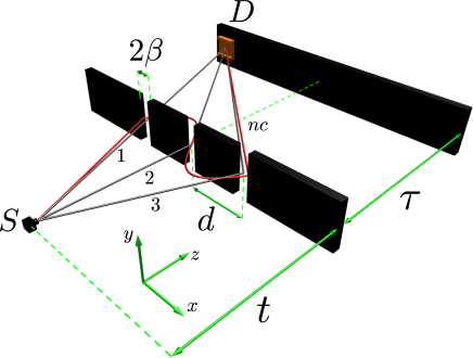
Figure 1: Sketch of triple-slit experiment. Gaussian wavepacket of transverse width $\sigma_{0}$ produced in the source $S$ propagates a time $t$ before attaining the triple-slit and a time $\tau$ from the triple-slit to the detector $D$. The slit apertures are taken to be Gaussian of width $\beta$ separated by a distance $d$.

The wave functions corresponding to the classical paths (grey lines) $1$ and $3$ read ($\int_{-\infty}^{+\infty}\ldots\int_{-\infty}^{+\infty}dx_{1}\ldots dx_{n}\equiv\int_{x_{1}\ldots x_{n}}$):

$$\psi_{1,3}(x,t,\tau) = \int_{x_{j},x_{0}}K_{\tau}(x,t+\tau;x_{j},t)F(x_{j}\pm d)$$ (1)

$$\times K_{t}(x_{j},t;x_{0},0)\psi_{0}(x_{0}),$$

whereas for the classical path $2$

$$\psi_{2}(x,t,\tau) = \int_{x_{j},x_{0}}K_{\tau}(x,t+\tau;x_{j},t)F(x_{j})$$ (2)

$$\times K_{t}(x_{j},t;x_{0},0)\psi_{0}(x_{0}),$$

with

$$K(x_{j},t_{j};x_{0},t_{0})=\sqrt{\frac{m}{2\pi i\hbar(t_{j}-t_{0})}}\exp\left[\frac{im(x_{j}-x_{0})^{2}}{2\hbar(t_{j}-t_{0})}\right],$$ (3)

$$F(x_{j})=\exp\left[-\frac{(x_{j})^{2}}{2\beta^{2}}\right],$$ (4)

and

$$\psi_{0}(x_{0})=\frac{1}{\sqrt{\sigma_{0}\sqrt{\pi}}}\exp\left(-\frac{x_{0}^{2}}{2\sigma_{0}^{2}}\right).$$ (5)

The kernels $K_{t}(x_{j},t;x_{0},0)$ and $K_{\tau}(x,t+\tau;x_{j},t)$ are the free propagators for the particle, the functions $F(x_{j})$ describe the slit transmission functions which are taken to be Gaussian of width $\beta$ separated by a distance $d$; $\sigma_{0}$ is the effective width of the wavepacket emitted from the source $S$, $m$ is the mass of the particle, $t$ ($\tau$) is the time of flight from the source (triple-slit) to the triple-slit (screen). The wavefunction associated with the non-classical path (red line) is given by

$$\psi_{nc}(x,t,\tau) = \int_{x_{0},x_{1},x_{2},x_{3}}K_{\tau}(x,\tau+\tilde{t};x_{3},\tilde{t})$$ (6)

$$\times F(x_{3}+d)F(x_{2})K(1\rightarrow 2;2\rightarrow 3)$$

$$\times F(x_{1}-d)K_{t}(x_{1},t+\alpha;x_{0},0)\psi_{0}(x_{0}),$$

where $\tilde{t}=t+2(\epsilon+\alpha)$ and

$$K(1\rightarrow 2;2\rightarrow 3)=\sqrt{\frac{m}{4\pi i\hbar(\epsilon+\alpha)}}\times$$

$$\exp\left[\frac{im[(x_{2}-x_{1})^{2}+(x_{3}-x_{2})^{2}]}{4\hbar(\epsilon+\alpha)}\right],$$ (7)

is the free propagator which propagates from slit $1$ to slit $2$ and from slit $2$ to slit $3$. The parameter $\alpha\rightarrow 0$ is an auxiliary inter slit time parameter and $\epsilon$ is the time spent from one to the next slit and is determined by the momentum uncertainty in the $x$-direction, i.e., $\epsilon=\frac{d}{\Delta v_{x}}$ ($\Delta v_{x}=\Delta p_{x}/m$), where $\Delta p_{x}=\sqrt{\langle\hat{p}^{2}_{x}\rangle-\langle\hat{p}_{x}\rangle^{2}}$, $\hat{p}_{x}$ being the momentum operator in the $x$-direction. This estimation is compatible with the propagation which builds the non-classical trajectory. A similar argument was used in Vedral , where non-classical dynamics based on uncertainty principle are considered in a interferometer. Trajectories winding around the slits evidently contribute less and less to the interference pattern.

After some lengthy algebraic manipulations, we obtain

$$\psi_{1}(x,t,\tau)=A\exp(-C_{1}x^{2}-C_{2}x+C_{3})\times$$

$$\exp(i\alpha x^{2}-i\gamma x-i\theta_{c}+i\mu_{c}),$$ (8)

$$\psi_{2}(x,t,\tau)=A\exp(-C_{1}x^{2})\exp(i\alpha x^{2}+i\mu_{c}),$$ (9)

$$\psi_{3}(x,t,\tau)=A\exp(-C_{1}x^{2}+C_{2}x+C_{3})\times$$

$$\exp(i\alpha x^{2}+i\gamma x-i\theta_{c}+i\mu_{c}),$$ (10)

and

$$\psi_{nc}(x,t,\tau)=A_{nc}\exp(-C_{1nc}x^{2}+C_{2nc}x+C_{3nc})\times$$

$$\exp\left(i\alpha_{nc}x^{2}+i\gamma_{nc}x-i\theta_{nc}+i\mu_{nc}\right),$$ (11)

where the non trivial Gouy phase $\mu_{nc}$ is given by

$$\mu_{nc}(t,\tau)=\frac{1}{2}\arctan\left(\frac{z_{I}}{z_{R}}\right).$$ (12)

All the coefficients present in equations (8)-(12) are written out in appendices 1 and 2 for the sake of clarity. The indices $R$ and $I$ stand for the real and imaginary part of the complexes numbers that appear in the solutions. As discussed in Paz2 , $\mu_{nc}(t,\tau)$ and $\theta_{nc}(t,\tau)$ are phases that do not depend of the transverse position $x$. Different from the Gouy phase, $\theta_{nc}(t,\tau)$ is one phase that appears as we displace the slit from a given distance of the origin, which is dependent on the parameter $d$.

The intensity at the screen including non-classical path reads

$$I_{nc} = |\psi_{1}+\psi_{2}+\psi_{3}+\psi_{nc}|^{2}$$ (13)

$$= I_{c}+|\psi_{nc}|^{2}+2|\psi_{1}||\psi_{nc}|\cos\phi_{1nc}$$

$$+ 2|\psi_{2}||\psi_{nc}|\cos\phi_{2nc}+2|\psi_{3}||\psi_{nc}|\cos\phi_{3nc},$$

where

$$\phi_{1nc}=(\alpha-\alpha_{nc})x^{2}-(\gamma+\gamma_{nc})x-(\theta_{c}-\theta_{nc})+(\mu_{c}-\mu_{nc}),$$ (14)

$$\phi_{2nc}=(\alpha-\alpha_{nc})x^{2}-\gamma_{nc}x+\theta_{nc}+(\mu_{c}-\mu_{nc}),$$ (15)

and

$$\phi_{3nc}=(\alpha-\alpha_{nc})x^{2}+(\gamma-\gamma_{nc})x-(\theta_{c}-\theta_{nc})+(\mu_{c}-\mu_{nc})$$ (16)

are the relative phases of $\psi_{1}$ and $\psi_{nc}$, $\psi_{2}$ and $\psi_{nc}$ and $\psi_{3}$ and $\psi_{nc}$, respectively, which implies that the interference is a result of two-paths as observed in Park . $I_{c}$ is the intensity when only classical paths are taken into account.

To quantify the deviations in the intensity produced by the existence of non-classical paths we use the Sorkin parameter as defined in Refs. Sinha2 ; Sinha3 , i.e.,

$$\kappa I_{0} = I_{nc}-I_{c}$$ (17)

$$= |\psi_{nc}|^{2}+2|\psi_{1}||\psi_{nc}|\cos\phi_{1nc}$$

$$+ 2|\psi_{2}||\psi_{nc}|\cos\phi_{2nc}+2|\psi_{3}||\psi_{nc}|\cos\phi_{3nc},$$

where $I_{0}$ is the intensity at central maximum. As we can observe the parameter $\kappa$ used to estimate the existence of non-classical path in the triple-slit interference is dependent of the Gouy phase difference between classical and non-classical paths.

III III. Sorkin parameter and Gouy phase for electron waves

In this section we analyse the Gouy phase effect in the quantity $\kappa$ for electron waves. Firstly we observe the behavior of the normalized intensity and the parameter $\kappa$ as a function of $x$ fixing the values of $t$ and $\tau$. We observe a displacement in the behavior of $\kappa$ as an effect of the Gouy phase which make clear the role of this phase in the exact estimation of $\kappa$. Secondly we observe the behavior of the parameter $\kappa$ as a function of $x$ and $\tau$ fixing the value of $t$ in which we can observe an upper bound for a given value of $x$ and $\tau$. Thirdly we consider the position $x=0$ and observe the behavior of the parameter $\kappa$ as a function of $\tau$ for $t$ fixed. For $x=0$ the Gouy phase effect is most evident since some other phases disappear in the interference as we can see in equations (14)-(16). As a matter of fact we can study the effect of all phases that appear with the non-classical path since we know the analytic expression for them, but we analyse here only the Gouy phase effect which can be measured for matter waves. Moreover it is possible to tune the parameters $t$ and $\tau$, $\sigma_{0}$, $\beta$ and $d$ in order to study a specific phase contribution.

To construct the graphic of the intensity and the Sorkin parameter $\kappa$ we consider an electron wave with the following parameters: $m=9.11\times 10^{-31}\;\mathrm{kg}$, $d=650\;\mathrm{nm}$, $\beta=62\;\mathrm{nm}$, $\sigma_{0}=62\;\mathrm{nm}$, $t=18\;\mathrm{ns}$, $\tau=15\;\mathrm{ns}$. Using these parameters as input we find $\epsilon=0.492ns$. In Fig. 2(a) we show the normalized intensity $I_{n}$ as a function of $x$ which shows the shape of intensity at far field or Fraunhofer theory as similarly observed in Sinha2 ; Raedt . In Fig. 2(b) we show the Sorkin parameter $\kappa$ as a function of $x$ in which we consider (solid line) and we do not consider (dotted line) the Gouy phase effect. In accordance with Sinha2 we find that the quantity $\kappa$ is of order $10^{-8}$ which corroborates our simplified analysis. Moreover we verify numerically that the factor $|\psi_{nc}(x,t,\tau)|^{2}$ does not change the parameter $\kappa$ significantly, the main contributions coming from the crossed terms which contain the Gouy phase.

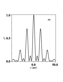
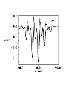
Figure 2: (a) Normalized intensity as a function of $x$. (b) Sorkin parameter $\kappa$ as a function of $x$. For solid line we consider and for dotted line we do not consider the Gouy phase difference.

In Fig. 3 we show the behavior of $|\kappa|$ as function of $x$ and $\tau$. We observe that it has a maximum for a given value of $x$ and $\tau$. The existence of a maximum enable us choose a set of value of parameters that produce a value of $\kappa$ which can be more accessible to be measured. The existence of a maximum value for this parameter as a function of the quantities involved in the experimental apparatus was previously observed in Sinha3 . As we can see this maximum occurs around $x=0$. Next we will explore the Gouy phase effect to estimate the parameter $\kappa$ for $x=0$ since for this position some phases disappear making the Gouy phase effect most evident.

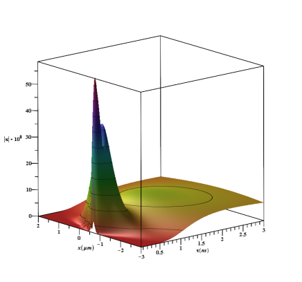
Figure 3: Absolute value of Sorkin parameter $\kappa$ as a function of $\tau$ and $x$ for $t$ fixed. It presents a maximum value for a given value of $x$ and $\tau$.

In figure 4(a) we show the Gouy phase of classical path (red line) and non-classical path (black line) as a function of $\tau$ for the same parameters used above. We can observe that the absolute value of the Gouy phase for the classical path decreases whereas for the non-classical path it increases as the time propagation $\tau$ grows. This change affects the parameter $\kappa$. To observe such effect, in Fig. 4(b) we show the absolute value of the parameter $\kappa$ as a function of $\tau$ for $x=0$.

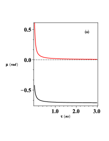
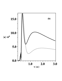
Figure 4: (a) Gouy phase difference as a function of $\tau$ and $t$ fixed. (b) Absolute value of Sorkin parameter $\kappa$ as a function of $\tau$ at $x=0$ and $t$ fixed.

The behavior of the parameter $\kappa$ as a function of $\tau$ is similar with that obtained as a function of the distance of the triple-slit to the screen in Sinha3 . For a given value of $\tau$ it has a peak as in Ref. Sinha3 . It is noteworthy that an exact solution for $\kappa$ depends on the Gouy phase. In order to evaluate the effect of the Gouy phase on the absolute value of the parameter $\kappa$, we calculate for point $x=0$ the percentage error which is defined by $(||\kappa|-|\kappa^{\prime}||/|\kappa|)\times 100\%$, where for $|\kappa|$ we consider the Gouy phase difference which corresponds to the exact value and for $|\kappa^{\prime}|$ we neglected the Gouy phase difference. Choosing $\tau=2\;\mathrm{ns}$ the percentage error is $51.5\%$. Therefore if the Gouy phase is neglected the parameter $\kappa$ is misestimated. As we can observe in figure 4(a) for $\tau=2\;\mathrm{ns}$ the Gouy phase of classical path tends to zero and the Gouy phase difference is due to the phase of the non-classical path contribution , i.e., $\mu_{c}-\mu_{nc}\approx|\mu_{nc}|\approx 0.719\;\mathrm{rad}$. If one uses these parameters one measures the Gouy phase difference as a signature of non-classical path contributions.

IV IV. Concluding remarks

We studied the effects of non-classical path in the interference pattern in a triple-slit experiment. We solved exactly a one dimensional model of propagation through a triple-slit and found analytical expressions for the wavefunctions of classical and non-classical paths. We obtained an exactly solution for the Sorkin parameter $\kappa$ used to estimate the effect of non-classical path. The value of $\kappa$ for electron waves is consistent with other results previously obtained for it which make our model reasonably good to study the existence of non-classical path. We used the uncertainty in momentum to estimate the inter slits propagation linking the existence of non-classical path with the uncertainty principle which is as intuitive as to appeal to Feynman’s path integral formalism. The Gouy phase of classical and non-classical paths are different which contribute significantly for the value of $\kappa$. We observed the changing in the behavior of $\kappa$ as a consequence of the Gouy phase difference for electron waves. We estimated the percentage error in the absolute value of parameter $\kappa$ as a consequence of the Gouy phase difference for $x=0$ and $\tau=2\;\mathrm{ns}$ and found $51.5\%$. We conclude, from the enormous discrepancy found, that the Gouy phase difference can not be neglected in the three-slit interference if non-classical paths are presents. We expected that our results which connect the Sorkin parameter and Gouy phase must be further useful to detect non-classical path’s effect by measuring the Gouy phase.

V appendix 1: Formulae for interference parameters

In the following we display the complete expressions of terms in eqs. (8), (9), (10) and (11):

$$A = \frac{m}{2\hbar\sqrt{\sqrt{\pi}t\tau\sigma_{0}}}\Bigg{[}\left(\frac{m^{2}}{4\hbar^{2}t\tau}-\frac{1}{4\beta^{2}\sigma_{0}^{2}}\right)^{2}$$ (18)

$$+ \frac{m^{2}}{16\hbar^{2}}\left(\frac{1}{\beta^{2}t}+\frac{1}{\sigma_{0}^{2}t}+\frac{1}{\sigma_{0}^{2}\tau}\right)^{2}\Bigg{]}^{-\frac{1}{4}},$$

$$C_{1}=\frac{\frac{m^{2}}{\hbar^{2}\tau^{2}}{\cal{A}}}{4\left[{\cal{A}}^{2}+{\cal{B}}^{2}\right]},$$ (19)

$$C_{2}=\frac{\frac{2md}{\hbar\tau\beta^{2}}{\cal{B}}}{4\left[{\cal{A}}^{2}+{\cal{B}}^{2}\right]},$$ (20)

$${\cal{A}}=\left(\frac{1}{2\beta^{2}}+\frac{m^{2}\sigma_{0}^{2}}{2(\hbar^{2}t^{2}+m^{2}\sigma_{0}^{4})}\right)$$

$${\cal{B}}=\left(\frac{m^{3}\sigma_{0}^{4}}{2\hbar t(\hbar^{2}t^{2}+m^{2}\sigma_{0}^{4})}-\frac{m}{2\hbar t}-\frac{m}{2\hbar\tau}\right)$$

$$C_{3}=-\frac{d^{2}}{2\beta^{2}}+\frac{\hbar^{2}\tau^{2}d^{2}}{m^{2}\beta^{2}}C_{1},\;\;\gamma=\frac{2d\hbar\tau}{m\beta^{2}}C_{1},$$

$$\alpha=\frac{mx^{2}}{2\hbar\tau}+\frac{m\beta^{2}}{2\hbar\tau}C_{2},\;\;\theta_{C}=\frac{\hbar\tau d}{2m\beta^{2}}C_{2},$$ (21)

$$\mu_{c}(t,\tau)=-\frac{1}{2}\arctan\left[\frac{t+\tau(1+\frac{\sigma_{0}^{2}}{\beta^{2}})}{\tau_{0}(1-\frac{t\tau\sigma_{0}^{2}}{\tau_{0}^{2}\beta^{2}})}\right],$$ (22)

$$A_{nc}=\sqrt{\frac{m^{3}\sqrt{\pi}}{16\hbar^{3}\tau t\epsilon\sigma_{0}\sqrt{z_{R}^{2}+z_{I}^{2}}}},$$ (23)

$$C_{1nc}=\frac{m^{2}z_{3R}}{4\hbar^{2}\tau^{2}(z_{3R}^{2}+z_{3I}^{2})},$$ (24)

$$C_{2nc}=\frac{m^{3}dz_{6I}}{32\hbar^{3}\beta^{2}\tau\epsilon^{2}(z_{6R}^{2}+z_{6I}^{2})}+\frac{mdz_{3I}}{2\hbar\tau\beta^{2}(z_{3R}^{2}+z_{3I}^{2})},$$ (25)

$$C_{3nc} = \frac{d^{2}z_{1R}}{4\beta^{4}(z_{1R}^{2}+z_{1I}^{2})}-\frac{m^{2}d^{2}z_{4R}}{64\beta^{4}\hbar^{2}\epsilon^{2}(z_{4R}^{2}+z_{4I}^{2})}$$ (26)

$$+ \frac{m^{4}d^{2}z_{5R}}{4^{5}\hbar^{4}\beta^{4}\epsilon^{4}(z_{5R}^{2}+z_{5I}^{2})}+\frac{m^{2}d^{2}z_{6R}}{32\beta^{4}\epsilon^{2}\hbar^{2}(z_{6R}^{2}+z_{6I}^{2})}$$

$$+ \frac{d^{2}z_{3R}}{4\beta^{4}(z_{3R}^{2}+z_{3I}^{2})}-\frac{d^{2}}{\beta^{2}},$$

$$\alpha_{nc}=\frac{mx^{2}}{2\hbar\tau}+\frac{m^{2}z_{3I}}{4\hbar^{2}\tau^{2}(z_{3R}^{2}+z_{3I}^{2})},$$ (27)

$$\gamma_{nc}=\frac{m^{3}dz_{6R}}{32\hbar^{3}\beta^{2}\tau\epsilon^{2}(z_{6R}^{2}+z_{6I}^{2})}+\frac{mdz_{3R}}{2\hbar\tau\beta^{2}(z_{3R}^{2}+z_{3I}^{2})},$$ (28)

$$\theta_{nc} = \frac{d^{2}z_{1I}}{4\beta^{4}(z_{1R}^{2}+z_{1I}^{2})}-\frac{m^{2}d^{2}z_{4I}}{64\beta^{4}\hbar^{2}\epsilon^{2}(z_{4R}^{2}+z_{4I}^{2})}$$ (29)

$$+ \frac{m^{4}d^{2}z_{5I}}{4^{5}\hbar^{4}\beta^{4}\epsilon^{4}(z_{5R}^{2}+z_{5I}^{2})}+\frac{m^{2}d^{2}z_{6I}}{32\beta^{4}\epsilon^{2}\hbar^{2}(z_{6R}^{2}+z_{6I}^{2})}$$

$$+ \frac{d^{2}z_{3I}}{4\beta^{4}(z_{3R}^{2}+z_{3I}^{2})},$$

VI appendix 2: Gouy phase components

In the following we present the full expression of the terms in equation (12).

$$z_{R} = (z_{0R}z_{1R}-z_{0I}z_{1I})(z_{2R}z_{3I}+z_{2I}z_{3R})+$$ (30)

$$+ (z_{0R}z_{1I}+z_{0I}z_{1R})(z_{2R}z_{3R}-z_{2I}z_{3I}),$$

$$z_{I} = (z_{0R}z_{1R}-z_{0I}z_{1I})(z_{2R}z_{3R}-z_{2I}z_{3I})$$ (31)

$$- (z_{0R}z_{1I}+z_{0I}z_{1R})(z_{2R}z_{3I}+z_{2I}z_{3R}),$$

$$z_{0R}=\frac{1}{2\sigma_{0}^{2}},\;\;z_{0I}=-\frac{m}{2\hbar t},$$ (32)

$$z_{1R}=\frac{1}{2\beta^{2}}+\frac{m^{2}z_{0R}}{4\hbar^{2}t^{2}(z_{0R}^{2}+z_{0I}^{2})},\;\;$$ (33)

$$z_{1I}=-\left(\frac{m}{4\hbar\epsilon}+\frac{m}{2\hbar t}+\frac{m^{2}z_{0I}}{4\hbar^{2}t^{2}(z_{0R}^{2}+z_{0I}^{2})}\right),$$ (34)

$$z_{2R}=\frac{1}{2\beta^{2}}+\frac{m^{2}z_{1R}}{16\hbar^{2}\epsilon^{2}(z_{1R}^{2}+z_{1I}^{2})},$$ (35)

$$z_{2I}=-\left(\frac{m}{2\hbar\epsilon}+\frac{m^{2}z_{1I}}{16\hbar^{2}\epsilon^{2}(z_{1R}^{2}+z_{1I}^{2})}\right),$$ (36)

$$z_{3R}=\frac{1}{2\beta^{2}}+\frac{m^{2}z_{2R}}{16\hbar^{2}\epsilon^{2}(z_{2R}^{2}+z_{2I}^{2})},$$ (37)

$$z_{3I}=-\left(\frac{m}{2\hbar\tau}+\frac{m}{4\hbar\epsilon}+\frac{m^{2}z_{2I}}{16\hbar^{2}\epsilon^{2}(z_{2R}^{2}+z_{2I}^{2})}\right),$$ (38)

$$z_{4R}=z_{1R}^{2}z_{2R}-z_{1I}^{2}z_{2R}-2z_{1R}z_{1I}z_{2I},$$ (39)

$$z_{4I}=z_{1R}^{2}z_{2I}-z_{1I}^{2}z_{2I}+2z_{1R}z_{1I}z_{2R},$$ (40)

$$z_{5R}=z_{3R}\big{(}z_{1R}^{2}z_{2R}^{2}-z_{1R}^{2}z_{2I}^{2}-z_{1I}^{2}z_{2R}^{2}+z_{1I}^{2}z_{2I}^{2}$$

$$-4z_{1R}z_{1I}z_{2R}z_{2I}\big{)}-2z_{3I}\big{(}z_{1R}^{2}z_{2R}z_{2I}-z_{1I}^{2}z_{2R}z_{2I}$$

$$+z_{1R}z_{1I}z_{2R}^{2}-z_{1R}z_{1I}z_{2I}^{2}\big{)},$$ (41)

$$z_{5I}=z_{3I}(z_{1R}^{2}z_{2R}^{2}-z_{1R}^{2}z_{2I}^{2}-z_{1I}^{2}z_{2R}^{2}+z_{1I}^{2}z_{2I}^{2}$$

$$-4z_{1R}z_{1I}z_{2R}z_{2I})+2z_{3R}(z_{1R}^{2}z_{2R}z_{2I}$$

$$-z_{1I}^{2}z_{2R}z_{2I}+z_{1R}z_{1I}z_{2R}^{2}-z_{1R}z_{1I}z_{2I}^{2}),$$ (42)

$$z_{6R}=z_{1R}z_{2R}z_{3R}-z_{1R}z_{2I}z_{3I}-z_{1I}z_{2R}z_{3I}-z_{1I}z_{2I}z_{3R},$$ (43)

and

$$z_{6I}=z_{1R}z_{2R}z_{3I}+z_{1R}z_{2I}z_{3R}+z_{1I}z_{2R}z_{3R}-z_{1I}z_{2I}z_{3I}.$$ (44)

References

(1)
L. G. Gouy, C. R. Acad. Sci. Paris 110, 1251 (1890).
(2)
L. G. Gouy, Ann. Chim. Phys. Ser. 6 24, 145 (1891).
(3)
T. D. Visser and E. Wolf, Opt. Comm. 283, 3371 (2010).
(4)
R. Simon and N. Mukunda, Phys. Rev. Lett. 70, 880 (1993).
(5)
S. Feng and H. G. Winful, Opt. Lett. 26, 485 (2001).
(6)
J. Yang and H. G. Winful, Opt. Lett. 31, 104 (2006).
(7)
R. W. Boyd, J. Opt. Soc. Am. 70, 877 (1980).
(8)
P. Hariharan and P. A. Robinson, J. Mod. Opt. 43, 219
(1996).
(9)
S. Feng, H. G. Winful, and R. W. Hellwarth, Opt. Lett.
23, 385 (1998).
(10)
X. Pang, T. D. Visser, and E. Wolf, Opt. Comm. 284, 5517
(2011); X. Pang, G. Gbur, and T. D. Visser, Opt. Lett.
36, 2492 (2011); X. Pang, D. G. Fischer, and T. D. Visser,
J. Opt. Soc. Am. A 29, 989 (2012); X. Pang and T. D.
Visser, Opt. Exp. 21, 8331 (2013); X. Pang, D. G.
Fischer, and T. D. Visser, Opt. Lett. 39, 88 (2014).
(11)
C. J. S. Ferreira, L. S. Marinho, T. B. Brasil, L. A. Cabral, J. G.
G. de Oliveira Jr, M. D. R. Sampaio, and I. G. da Paz, Ann. of
Phys. 362, 473 (2015).
(12)
D. Chauvat, O. Emile, M. Brunel, and A. Le Floch, Am. J. Phys.
71, 1196 (2003).
(13)
N. C. R. Holme, B. C. Daly, M. T. Myaing, and T. B. Norris, Appl.
Phys. Lett. 83, 392 (2003).
(14)
W. Zhu, A. Agrawal, and A. Nahata, Opt. Exp. 15, 9995
(2007).
(15)
T. Feurer, N. S. Stoyanov, D. W. Ward, and K. A. Nelson, Phys. Rev.
Lett. 88, 257 (2002).
(16)
A. Hansen, J. T. Schultz, and N. P. Bigelow, Conference on
Coherence and Quantum Optics Rochester (New York, United States,
2013); J. T. Schultz, A. Hansen, and N. P. Bigelow, Opt. Lett.
39, 4271 (2014).
(17)
G. Guzzinati, P. Schattschneider, K. Y. Bliokh, F. Nori, and J.
Verbeeck, Phys. Rev. Lett. 110, 093601 (2013).
(18)
T. C. Petersen, D. M. Paganin, M. Weyland, T. P. Simula, S. A.
Eastwood, and M. J. Morgan, Phys. Rev. A 88, 043803
(2013).
(19)
A. E. Siegman, Lasers, University Science Books, Sausalito CA, 1986.
(20) Ph. Balcou and A. L.
Huillier, Phys. Rev. A 47, 1447 (1993); M. Lewenstein,
P. Salieres, and A. L. Huillier, Phys. Rev. A 52, 4747
(1995); F. Lindner, W. Stremme, M. G. Schatzel, F. Grasbon, G. G.
Paulus, H. Walther, R. Hartmann, and L. Struder, Phys. Rev. A
68, 013814 (2003).
(21) F. Lindner, G. Paulus, H. Walther, A. Baltuska, E. Goulielmakis, M. Lezius, and F. Krausz, Phys. Rev. Lett.
92, 113001 (2004).
(22) L. Allen, M. W. Beijersbergen, R.J.C. Spreeuw, and
J.P. Woerdman, Phys. Rev. A 45, 8185 (1992); L. Allen, M.
Padgett, and M. Babiker, Prog. Opt. 39, 291 (1999).
(23)
S. Sato and S. Kawamura, Journal of Physics: Conference Series
122, 012025 (2008).
(24)
I. G. da Paz, M. C. Nemes , S. Padua, C. H. Monken, and J.G. Peixoto
de Faria, Phys. Lett. A 374, 1660 (2010).
(25)
I. G. da Paz, P. L. Saldanha, M. C. Nemes, and J. J. Peixoto de
Faria, New J. of Phys. 13, 125005 (2011).
(26)
R. Ducharme and I. G. da Paz, Phys. Rev. A 92, 023853
(2015).
(27)
H. Yabuki, Int. J. Theor. Ph. 25, 159 (1986).
(28)
R. P. Feynman and A. R. Hibbs, Quantum Mechanics and Path
Integrals (McGraw-Hill, New York, 3rd. ed. 1965).
(29)
R. D. Sorkin, Mod. Phys. Lett. A 09, 3119 (1994).
(30)
U. Sinha, C. Couteau, T. Jennewein, R. Laflamme, and G. Weihs,
Science 329, 418 (2010).
(31)
H. D. Raedt, K. Michielsen, and K. Hess, Phys. Rev. A 85,
012101 (2012).
(32)
R. Sawant, J. samuel, A. Sinha, S. Sinha, and U. Sinha, Phys. Rev.
Lett. 113, 120406 (2014).
(33)
A. Sinha, A. H. Vijay, and U. Sinha, Scientific Reports
5, 10304 (2015).
(34)
J. S. M. Neto, L. A. Cabral, and I. G. da Paz, Eur. J. Phys.
36, 035002 (2015).
(35)
O. C. O. Dahlsten, A. J. P. Garner, and V. Vedral, Nat. Commun.
5, 4592 (2014).
(36)
D. K. Park, O. Moussa, and R. Laflamme, New. J. of Phys.
14, 113025 (2012).