An Entropy-Based Technique for Classifying Bacterial Chromosomes According to Synonymous Codon Usage

Abstract

We present a framework based on conditional entropy and the Dirichlet distribution for classifying chromosomes based on the degree to which they use synonymous codons uniformly or preferentially, that is, whether or not codons that code for an amino acid appear with the same relative frequency. Applying the approach to a large collection of annotated bacterial chromosomes reveals three distinct groups of bacteria.

Keywords: entropy; conditional entropy; Dirichlet distribution; annotated bacteria.

Mathematics Subject Classification (2010): 60F10; 60G42; 92D20; 62P10.

1 Introduction

Living cells use the genetic code to translate triples of nucleic acids called codons into amino acids, the building blocks of proteins. There are a total of 64 codons of which 61 code for 20 amino acids while the remaining 3 constitute translation stop signals. This many-to-one mapping between codons and amino acids means the genetic code is degenerate. As almost all amino acids are represented by two to six different codons, the code possesses intrinsic redundancy. this provides the cellular machinery with the ability to correctly manufacture protein products in the presence of certain kinds of transcription/translation/replication errors. However, the way in which codons are used to represent amino acids varies from gene to gene and from organism to organism. The mechanism by which variations in these usage patterns arise is not clearly understood, though a number of factors that can influence codon usage are known. these include mutational biases, translational selection pressures, GC content at the third codon site (GC3s) and gene size. The pattern in the way amino acids are represented by codons is called synonymous codon usage (SCU) and inequity in the distribution of codons which code for the same amino acid is referred to as codon usage bias (CUB).

As noted above, patterns of SCU are specific to each organism and their study is of significant biological interest. Consequently, there is a substantial body of literature devoted to studying SCU in the genes of organisms. Comeron and Aguade (1998) give a brief review of methods for measuring SCU, both general and species-specific. Two useful measures are the codon adaptation index (Sharp and Li, 1987) and the ‘effective number of codons’ (Wright, 1990). A number of other measures have been subsequently posed such as relative codon adaptation (Fox and Erill, 2010), various modifications to the ‘effective number of codons’ (Fuglsang, 2006; Banerjeee et al., 2005) and the measure of gene expression $E(G)$ which was used by Karlin et al. (2001) to characterize predicted highly expressed genes in four bacteria.

Here, we develop a method for assessing codon usage bias based on concepts taken from information theory and apply it to a large set of bacterial chromosomes. As our aim is to explore and identify trends in global SCU in a large collection of organisms, our approach differs from that which is typically taken when studying SCU in a chromosome. Rather than examining a chromosome gene by gene, we aggregate all the genes annotated for the chromosome together and compute total relative frequencies for codons and amino acids which are then plugged into our measure.

To set the scene more concretely, let $\{\hbox{\rm A},\hbox{\rm C},\hbox{\rm G},\hbox{\rm T}\}$ be the alphabet of nucleotides in DNA. Being triplets of nucleotides, codons are elements of $\{\hbox{\rm A},\hbox{\rm C},\hbox{\rm G},\hbox{\rm T}\}^{3}$ and $61$ of the $64$ possible codons code for amino acids. The remaining $3$ codons (TAA, TAG and TGA) indicate a STOP condition that is transcribed into messenger RNA and which instructs the ribosome to halt the translation of a sequence of codons into a polypeptide chain.

Each amino acid can be represented by any of its so-called synonymous codons, which are those codons that code for it. For instance, the four codons GCA, GCG, GCT and GCC all code for the amino acid alanine (Ala). Thus the list of amino acids defines a partition $\alpha^{*}=\{A^{*}_{d}:d=1,..,20\}$ on the set of $61$ codons. Each amino acid is associated with a class $A^{*}_{d}$ which is the set of its synonymous codons. For example, if $A_{1}^{*}$ corresponds to Ala, then $A_{1}^{*}=\{\text{GCA},\text{GCG},\text{GCT},\text{GCC}\}$. Further, the collection of $20$ amino acids can be organized according to the number of synonymous codons each has: there are $5$ amino acids with $4$ synonymous codons, $3$ with $6$ codons, $9$ with $2$ codons, $1$ with $3$ codons and $2$ with just $1$ codon.

We seek a measure or statistic $\Delta$ that captures the degree to which the set of amino acids are represented equally often by their synonymous codons. If we suppose that there are $k_{d}$ codons that code for amino acid $A_{d}$, then $A_{d}$ will exhibit no CUB if each of its $k_{d}$ synonymous codons appears with relative frequency $1/k_{d}$. Extending this, it should be clear that a complete chromosome will exhibit no CUB provided that every codon $C$ appears in the chromosome with a relative frequency equal to the reciprocal of the number of codons that code for the same amino acid as $C$. In order for  $\Delta$ to be useful, it should possess a number of desirable properties. Firstly, a complete absence of CUB, the ideal case just described, should be indicated by the reference value of $0$. Secondly, the most extreme form of CUB where each amino acid is always represented by the same codon should correspond to the maximum value of $\Delta$. Thirdly, larger values of $\Delta$ should correspond to greater concentrations of the codon distribution on a smaller number of codons, with the extreme case being one codon per amino acid. Finally, it should be independent of the amino acid composition so that comparisons can be made between chromosomes and/or organisms.

The following sections develop such a measure in a very general framework, replacing the set of codons by an arbitrary finite set $I$ of symbols and the amino acid partition $\alpha^{*}$ by a general partition $\alpha$ of $I$. Section 2 begins by presenting information theoretic concepts such as partitions, entropy, conditional entropy and maximal entropy of probability measures when fixing a probability measure over some partition and defines a statistic $\Delta$ for CUB. The relationship of $\Delta$ to probabilistic measures such as the Kullback and $\chi^{2}$ distances is investigated. It is also compared to homozygosity, a well-known measure of genetic similarity. Section 3 deals with computing the mean entropy under a Dirichlet distribution assumption on the use of symbols belonging to the same atom. This enables the expected value of  $\Delta$ to be computed directly from the relative frequencies of the amino acids. In Section 4, we obtain some large deviation bounds with respect to the Dirichlet distribution assumption.

The final section applies the proposed entropy-based approach to a set of $2535$ annotated bacterial chromosomes and we discover that the bacteria can be divided into three broad groups based on their SCU behavior. In the largest group, which contains $1587$ bacteria, amino acids are represented uniformly by their synonymous codons. The next largest group consists of $592$ bacteria that exhibit a very high degree of CUB, indicating an extreme preference for a small number of codons. the third and smallest group has $356$ bacteria whose SCU bias is moderate.

2 Partitions, Entropy and Maximal Entropy

Let $I$ be a finite set and denote its cardinality by $|I|$. A partition $\alpha=(A:A\in\alpha)$ of $I$ is such that its elements, which we shall call atoms, are non-empty, disjoint and cover $I$, that is,

$$A\neq\emptyset\text{ for $A\in\alpha$}$$ (non-emptiness);

$$A\cap A^{\prime}=\emptyset\text{ for $A\neq A^{\prime}$, $A,A^{\prime}\in\alpha$}$$ (disjointness);

$$I=\bigcup_{A\in\alpha}A$$ (coverage).

For an element $i\in I$ we use $A^{i,\alpha}\in\alpha$ to denote the unique atom of $\alpha$ that contains $i$.

A partition $\beta=(B:B\in\beta)$ is said to be finer than $\alpha$ (or $\alpha$ is coarser than $\beta$), written $\beta\succeq\alpha$, if every atom of $\alpha$ is a union of atoms of $\beta$. Let $\beta\succeq\alpha$. For every $B\in\beta$ there is a unique atom $A\in\alpha$ containing $B$ and we denote this $A$ by $A^{B,\alpha}$. For $A\in\alpha$, we define

$$N^{\beta}(A)=|\{B\in\beta:B\subseteq A\}|,$$

the number of atoms of $\beta$ contained in $A$. So, for $B\in\beta$, $N^{\beta}(A^{B,\alpha})$ is the number of atoms of $\beta$ which are in the atom of $\alpha$ containing $B$. In the following, an increasing sequence of partitions should be understood to mean that the sequence of partitions is increasing with respect to the order $\preceq$.

The finest partition is the discrete one ${\cal D}=\{\{i\}:i\in I\}$ while the coarsest is the trivial one ${\cal N}=\{I\}$. Let $\sigma(\alpha)$ denote the field generated by partition $\alpha$, that is, the class of sets that are unions of atoms of $\alpha$. We denote the set of probability measures on $(I,\sigma(\alpha))$ by ${\cal P}(I,\sigma(\alpha))$.

Once and for all, we fix two partitions $\alpha$ and $\beta$ satisfying $\beta\succ\alpha$. Also we fix a probability distribution $q\in{\cal P}(I,\sigma(\alpha))$. This distribution can be represented by a vector $q=(q_{A}:A\in\alpha)$ satisfying $q_{A}\geq 0$ for $A\in\alpha$ and $\sum_{A\in\alpha}q_{A}=1$. Its Shannon entropy $h(\alpha,q)$ is given by

$$h(\alpha,q)=-\sum_{A\in\alpha}q_{A}\log q_{A}.$$ (1)

A probability measure $r\in{\cal P}(I,\sigma(\beta))$ extends $q$ if $r|_{\sigma(\alpha)}=q$, that is if $q_{A}=\sum_{B\in\beta:B\subseteq A}r_{B}$ for all $A\in\alpha$. We write this extension relation as $r\succeq q$. In this case we have the increasing property $h(\alpha,q)\leq h(\beta,r)$ and thus the conditional entropy is

$$h_{r}(\beta\,|\,\alpha)=h(\beta,r)-h(\alpha,q)=-\sum_{A\in\alpha}q_{A}\left(\sum_{B\in\beta:B\subseteq A}\frac{r_{B}}{q_{A}}\log\frac{r_{B}}{q_{A}}\right).$$ (2)

Denote the set of extensions of $Q$ by

$${\cal P}(I,\sigma(\beta)\,|\,q)=\{r\in{\cal P}(I,\sigma(\beta)):r\succeq q\}.$$

From now on, we shall assume that $r\in{\cal P}(I,\sigma(\beta)\,|\,q)$.

Next, define $r^{M}\in{\cal P}(I,\sigma(\beta))$ by

$$\forall B\in\beta:\quad r^{M}_{B}=N^{\beta}(A^{B,\alpha})^{-1}q_{A^{B,\alpha}},$$

that is, $r^{M}$ gives the same weight to the atoms of $\beta$ which are contained in the same atom of $\alpha$. An easy computation shows that $r^{M}\in{\cal P}(I,\sigma(\beta)\,|\,q)$ and its entropy is

$$h(\beta,r^{M})=\sum_{A\in\alpha}q_{A}\log N^{\beta}(A)+h(\alpha,q).$$

Since the function $-x\log x$ is concave on the interval $[0,1]$, Jensen’s inequality implies that $r^{M}$ maximizes the entropy over the set of probability measures that extend $q$, that is,

$$h(\beta,r^{M})=\max\{h(\beta,r):r\in{\cal P}(I,\sigma(\beta)\,|\,q)\}.$$

Once again letting $r\in{\cal P}(I,\sigma(\beta)\,|\,q)$, we define

$$\Delta^{q}(\beta,r)=h(\beta,r^{M})-h(\beta,r).$$ (3)

In other words, $\Delta^{q}(\beta,r)$ is the difference between the maximal conditional entropy over the partition $\beta$ and the entropy of $r$ over $\beta$, both extending $q$. Then,

$$\Delta^{q}(\beta,r) = \sum_{A\in\alpha}q_{A}\log N^{\beta}(A)+h(\alpha,q)-h_{r}(\beta\,|\,\alpha)-h(\alpha,q)$$ (4)

$$= \sum_{A\in\alpha}q_{A}\log N^{\beta}(A)-h_{r}(\beta\,|\,\alpha).$$

Now, the statistic $\Delta$ we shall use for assessing a genome’s CUB will be the special case of $\Delta^{q}(\beta,r)$ in which $\beta$ is set to the discrete partition of codons ${\cal D}$, that is,

$$\Delta=\Delta^{q}({\cal D},r).$$ (5)

As such, $\Delta$ is the difference between two entropies. The first is the maximum conditional entropy over the discrete partition ${\cal D}$ of codons for probability measures extending the amino acid composition $q$ and the second is the entropy of the codon distribution $r$ which also extends $q$.

This statistic satisfies a number of properties which make it useful for assessing CUB. Being based on entropy, it is a natural quantity for measuring departure from equal usage. It takes the value zero if and only if $r$ is constant on each atom of $\alpha$, a configuration concordant with unbiased SCU. The maximum value that $\Delta$ can take is $\sum_{A\in\alpha}q_{A}\log N^{\beta}(A)$. By the definition of $\Delta$, this maximum value corresponds to a conditional entropy of zero, that is, $h_{r}({\cal D}\,|\,\alpha)=0$, and this means there is precisely one codon representing each amino acid. Finally, fixing the distribution of amino acids in the definition of $\Delta$ has the effect of removing the influence of amino acid composition so that $\Delta$ can be used to compare the degree of CUB in coding sequences from different chromosomes/species.

2.1 Relationship to Kullback and $\chi^{2}$ distances

The quantity $\Delta^{q}(\beta,r)$ can be characterized in terms of the Kullback ‘distance’. We recall that if $\nu$ and $\mu$ are two probability measures on a measurable space with $\mu\ll\nu$ then the Kullback distance is $d_{\hbox{k}}(\mu,\nu)=\left(\int f\,\log f\,d\nu\right)^{1/2}$, where $f=d\mu/\,d\nu$ is the Radon-Nikodym derivative of $\mu$ with respect to $\nu$.

Proposition 1.

For $r\in{\cal P}(I,\sigma(\beta)\,|\,q)$, $\Delta^{q}(\beta,p)=d_{\hbox{k}}(r,r^{M})^{2}$.

Proof.

For $i\in B\in\beta$ we have

$$\frac{dr}{dr^{M}}(i)=N^{\beta}(A^{B,\alpha})\frac{r_{B}}{q_{A}},$$

so

$$d_{\hbox{k}}(r,r^{M})^{2}=\sum_{A\in\alpha}\sum_{B\in\beta:B\subseteq A}N^{\beta}(A^{B,\alpha})\frac{r_{B}}{q_{A}}\log\left(N^{\beta}(A^{B,\alpha})\frac{r_{B}}{q_{A}}\right)\frac{q_{A}}{N^{\beta}(A^{B,\alpha})}.$$

Then

$$d_{\hbox{k}}(r,r^{M})^{2} = h(\alpha,q)-h(\beta,r)+\sum_{A\in\alpha}\sum_{B\in\beta:B\subseteq A}r_{B}\log N^{\beta}(A)$$

$$= h(\alpha,q)-h(\beta,r)+\sum_{A\in\alpha}q_{A}\log N^{\beta}(A)=\Delta^{q}(\beta,r).$$

${}_{\blacksquare}$

Let us recall the $\chi^{2}$ distance, which in the setting of $\mu\ll\nu$ and $f=d\mu/\,d\nu$ satisfies $d_{\chi^{2}}(\mu,\nu)=\left(\int(f-1)^{2}d\nu\right)^{1/2}$. From a general formula (see Gibbs and Su, 2002), we have

$$d_{\hbox{k}}(\mu,\nu)\leq d_{\chi^{2}}(\mu,\nu).$$ (6)

In our case the $\chi^{2}$ distance is given by

$$d_{\chi^{2}}(r,r^{M})^{2} = \sum_{A\in\alpha}\sum_{B\in\beta:B\subseteq A}\left(N^{\beta}(A)\frac{r_{B}}{q_{A}}-1\right)^{2}\frac{q_{A}}{N^{\beta}(A^{B,\alpha})}$$

$$= \sum_{A\in\alpha}\frac{q_{A}}{N^{\beta}(A)}\sum_{B\in\beta:B\subseteq A}\left(N^{\beta}(A)\frac{r_{B}}{q_{A}}-1\right)^{2}$$

$$= \sum_{A\in\alpha}\frac{q_{A}}{N^{\beta}(A)}\left(\sum_{B\in\beta:B\subseteq A}\left(N^{\beta}(A)\frac{r_{B}}{q_{A}}\right)^{2}-2N^{\beta}(A)+N^{\beta}(A)\right)$$

$$= \sum_{A\in\alpha}\frac{q_{A}}{N^{\beta}(A)}\sum_{B\in\beta:B\subseteq A}\left(N^{\beta}(A)\frac{r_{B}}{q_{A}}\right)^{2}-1$$

$$= \sum_{A\in\alpha}q_{A}N^{\beta}(A)\sum_{B\in\beta:B\subseteq A}\left(\frac{r_{B}}{q_{A}}\right)^{2}-1.$$

The $\chi^{2}$ distance can be related to the homozygosities of the atoms of $\alpha$. Statistical estimators of homozygosity were used previously to construct a measure of CUB called the “effective number of codons” (Wright, 1990). The homozygosity of each atom $A\in\alpha$ is

$$\kappa_{A}(\beta)=\sum_{B\in\beta:B\subseteq A}\left(\frac{r_{B}}{q_{A}}\right)^{2}.$$

Then,

$$d_{\chi^{2}}(\mu,\nu)^{2}=\sum_{A\in\alpha}q_{A}N^{\beta}(A)\sum_{B\in\beta:B\subseteq A}\left(\frac{r_{B}}{q_{A}}\right)^{2}-1=\sum_{A\in\alpha}q_{A}N^{\beta}(A)\kappa_{A}(\beta)-1.$$

Consequently, from (6) we get $\Delta(\beta,r)\leq\sum_{A\in\alpha}q_{A}N^{\beta}(A)\kappa_{A}(\beta)-1$.

3 Conditional entropy on Dirichlet distributions

First, we write everything in terms of a probability measure $p\in{\cal P}(I,\sigma({\cal D}))$. This measure is characterized as a vector $p=(p_{i}:i\in I)$ which satisfies $p_{i}\geq 0$ for $i\in I$ and $\sum_{i\in I}p_{i}=1$. Then, $p(J)=\sum_{i\in J}p_{i}$ for $J\subseteq I$ and $p(\{i\})=p_{i}$.

We will take $p\in{\cal P}(I,\sigma({\cal D})\,|\,q)$ to be an extension of $q$. Let $r=p|_{\sigma(\beta)}$ be the restriction of $p$ to $\sigma(\beta)$ so $r\in{\cal P}(I,\sigma(\beta)\,|\,q)$. We write $h_{p}(\beta)=h_{r}(\beta)$, $h_{p}(\beta\,|\,\alpha)=h_{r}(\beta\,|\,\alpha)$ and $\Delta^{q}(\beta,p)=\Delta^{q}(\beta,r)$.

We would like to have an idea of how $\Delta^{q}(\beta,p)$ behaves probabilistically. Toward this end, we shall place a probability law on ${\cal P}(I,\sigma({\cal D})\,|\,q)$ that captures our a priori ignorance about the measure $p$ and compute $\Delta^{q}(\beta,p)$ when $p$ is chosen according to this law. Since the first term of $\Delta^{q}(\beta,p)$ in (4) does not depend on $p$, we need only examine the behavior of the quantity $h_{p}(\beta\,|\,\alpha)$.

To begin, note that any $p\in{\cal P}(I,\sigma({\cal D})\,|\,q)$ is an element of ${\cal P}(I,\sigma({\cal D}))$ which satisfies $\sum_{i\in A}p_{i}=q_{A}$ for $A\in\alpha$. So $p$ is characterized by the set of probability vectors of the form

$$\left(q_{A}^{-1}(p_{i}:i\in A):A\in\alpha\right).$$

Here $q_{A}^{-1}(p_{i}:i\in A)=(p_{i}/q_{A}:i\in A)$ is a probability vector that takes values in $S_{|A|-1}$, the simplex of dimension $|A|-1$.

We fix the distribution ${\mathbb{P}}$ on ${\cal P}(I,\sigma({\cal D})\,|\,q)$ as a product of Dirichlet distributions with its support constrained to the set of extensions of $q$. More precisely, the random vector $P=(P_{i}:i\in I)$ which takes values in ${\cal P}(I,\sigma({\cal D})\,|\,q)$ is such that

$$X(A)=q_{A}^{-1}(P_{i}:i\in A)\sim\,\text{Dirichlet}\,(\underbrace{1,..,1}_{|A|\,\text{times}}),$$ (7)

and $(X(A):A\in\alpha)$ are independent random vectors. We recall that the density for $(Y_{1},..,Y_{a})\sim\,\text{Dirichlet}\,(\underbrace{1,..,1}_{a\,\text{times}})$ is $f_{Y_{1},..,Y_{a}}(y_{1},..,y_{a})=(a-1)!{\bf 1}((y_{1},..,y_{a})\in S_{a-1})$.

We can now compute the value ${\mathbb{E}}\bigl{(}\Delta^{q}(\beta,P)\bigr{)}$ with respect to this distribution.

Theorem 2.

Fix a partition $\alpha$ and a probability distribution $q$ on $\alpha$. Let $\beta\succeq\alpha$ and let $P$ be a random probability vector in ${\cal P}(I,\sigma({\cal D})\,|\,q)$ which is distributed according to (7). Then

$${\mathbb{E}}(h_{P}(\beta\,|\,\alpha))=\sum_{A\in\alpha}q_{A}\xi_{|A|}-\sum_{A\in\alpha}\frac{q_{A}}{|A|}\left(\sum_{B\in\beta:B\subseteq A}|B|\xi_{|B|}\right),$$ (8)

where $\xi_{n}=\sum_{j=1}^{n}j^{-1}$ denotes the $n^{\rm th}$ harmonic number.

Proof.

To begin, we recall a standard construction of $(Y_{j}:j=1,..,a)\sim\,\text{Dirichlet}\,(c_{1},..,c_{a})$ for positive real numbers $c_{j}$, $j=1,..,a$ (see for instance Section 2.2.1 in Bertoin, 2006). We take independent random variables $G_{j},$ $j=1,..,a$ with $G_{j}$ distributed as Gamma$(c_{j},1)$. Then, $\bigl{(}G_{j}\big{/}\sum_{i=1}^{a}G_{i}:j=1,..,a\bigr{)}\sim\,$ Dirichlet$\,(c_{1},..,c_{a})$ which is independent of $\sum_{i=1}^{a}G_{i}\sim\,$Gamma$(\sum_{j=1}^{a}c_{j},1$).

Now, if $(Y_{j}:j=1,..,a)\sim\,$ Dirichlet$\,(c_{1},...,c_{a})$ with $c_{1},..,c_{a}>0$, $(J_{i}:i=1,..,k)$ is a partition of $\{1,..,a\}$ and $Z_{i}=\sum_{j\in J_{i}}Y_{j}$ for $i=1,..,k$, then it follows that $(Z_{i}:i=1,..,k)\sim\,$ Dirichlet$\,\left(\sum_{j\in J_{i}}c_{j}:i=1,..,k\right)$. As a special case of this, we have

$$(Z_{i},1-Z_{i})\sim\,\text{ Dirichlet }\left(\sum_{j\in J_{i}}c_{j},\sum_{j\in\{1,..,a\}\setminus J_{i}}c_{j}\right).$$ (9)

Recalling that $P(B)=\sum_{i\in B}P_{i}$, (2) yields

$$h_{P}(\beta\,|\,\alpha)=-\sum_{A\in\alpha}q_{A}\left(\sum_{B\in\beta:B\subseteq A}\frac{P(B)}{q_{A}}\,\log\frac{P(B)}{q_{A}}\right)$$

and combining distributions (7) and (9) enables us to conclude that

$$\left(\frac{P(B)}{q_{A}},1-\frac{P(B)}{q_{A}}\right)\sim\,\text{Dirichlet}(|B|,|A|-|B|)$$

for $B\in\beta$, $B\subseteq A\in\alpha$. Then,

$${\mathbb{E}}(h_{P}(\beta\,|\,\alpha))=-\sum_{A\in\alpha}q_{A}\left(\sum_{B\in\beta:B\subseteq A}{\mathbb{E}}(W_{B,A}\log W_{B,A})\right),$$ (10)

where $W_{B,A}\sim\hbox{Dirichlet}\,(|B|,|A|-|B|)$.

We need to compute ${\mathbb{E}}(W\log W)$ for $(W,1-W)\sim\,\text{Dirichlet}\,(l,m)$. Firstly,

$${\mathbb{E}}\left(W\,\log W\right)=\frac{(l+m-1)!}{(l-1)!\,(m-1)!}\int_{0}^{1}x\,(\log x)\,x^{l-1}(1-x)^{m-1}dx.$$

For integers $s,t\geq 0$, define

$$\theta(s,t)=\int_{0}^{1}x^{s}\,(1-x)^{t}\,\log x\,dx.$$

This notation allows us to write

$${\mathbb{E}}\left(W\log W\right)=\frac{(l+m-1)!}{l-1)!\,(m-1)!}\theta(l,m-1).$$

Thus, it is only necessary to compute $\theta(s,t)$, which will be done by successively integrating by parts and by making use of the formula

$$\frac{d}{dx}A_{s}(x)=x^{s}\log x\text{ where }A_{s}(x)=\frac{x^{s+1}\,\log x}{s+1}-\frac{x^{s+1}}{(s+1)^{2}}.$$

To begin, we have $A_{s}(0)=0$ and $A_{s}(1)=-\frac{1}{(s+1)^{2}}$. Next for $t=0$ we have $\theta(s,0)=A_{s}(x)|_{0}^{1}=-\frac{1}{(s+1)^{2}}$. Assume $t>0$. Since $A_{s}(x)(1-x)^{t}|_{0}^{1}=0$ we obtain

$$\theta(s,t)=t\int_{0}^{1}A_{s}(x)(1-x)^{t-1}dx=\frac{t}{s+1}\theta(s+1,t-1)-\frac{t}{(s+1)^{2}}\int_{0}^{1}x^{s+1}(1-x)^{t-1}dx\,.$$

If $t=1$ we obtain

$$\theta(s,1)=\frac{1}{s+1}\theta(s+1,0)-\frac{1}{(s+1)^{2}(s+2)}=-\frac{(2s+3)}{(s+1)^{2}(s+2)^{2}}\,.$$ (11)

If $t>1$ we find that

$$\theta(s,t) = \frac{t}{s+1}\theta(s+1,t-1)-\frac{t}{(s+1)^{2}}\frac{(s+1)!(t-1)!}{(s+1+t)!}$$

$$= \frac{t}{s+1}\theta(s+1,t-1)-\frac{1}{(s+1)}\frac{s!t!}{(s+1+t)!}.$$

Then by iterating and by using (11), we obtain

$$\theta(s,t) = \theta(s+t-1,1)\frac{s!\,t!}{(s+t-1)!}-\frac{s!\,t!}{(s+t+1)!}\left(\sum_{j=1}^{t-1}\frac{1}{s+j}\right)$$

$$= -\frac{(2(s+t)+1)}{(s+t)(s+t+1)}\frac{s!\,t!}{(s+t+1)!}-\frac{s!\,t!}{(s+t+1)!}\left(\sum_{j=1}^{t-1}\frac{1}{s+j}\right)$$

$$= -\frac{s!\,t!}{(s+t+1)!}\left(\frac{(2(s+t)+1)}{(s+t)(s+t+1)}+\sum_{j=1}^{t-1}\frac{1}{s+j}\right)$$

$$= -\frac{s!\,t!}{(s+t+1)!}\left(\sum_{j=1}^{t+1}\frac{1}{s+j}\right)=-\frac{s!\,t!}{(s+t+1)!}\left(\xi_{s+t+1}-\xi_{s}\right).$$

Hence, for $(W,1-W)\sim\,$Dirichlet$\,(l,m)$ we have

$${\mathbb{E}}(W\,\log W) = \frac{(l+m-1)!}{l-1)!\,(m-1)!}\theta(l,m-1)$$

$$= -\frac{(l+m-1)!}{(l-1)!\,(m-1)!}\cdot\frac{l!\,(m-1)!}{(l+m)!}\left(\xi_{l+m}-\xi_{l}\right)=-\frac{l}{l+m}\left(\xi_{l+m}-\xi_{l}\right).$$

Setting $W=W_{B,A}$, $l=|B|$ and $m=|A|-|B|$, we obtain

$${\mathbb{E}}(W_{B,A}\,\log W_{B,A})=-\frac{|B|}{|A|}\left(\xi_{|A|}-\xi_{|B|}\right)$$

and substituting this into (10) yields the result. ${}_{\blacksquare}$

Note. The calculations in the above proof also enable ${\mathbb{E}}\bigl{(}h_{P}(\beta\,|\,\alpha)\bigr{)}$ to be computed exactly when $X(A)\sim\,$Dirichlet $\,(\underbrace{c,..,c}\limits_{|A|\text{times}})$ where $c$ is a positive fixed integer which is the same for all $A\in\alpha$. Here, we have fixed $c=1$ in the statement of the theorem because this causes all distributions $p$ that extend $q$ to occur with the same probability.

Corollary 3.

We have

$${\mathbb{E}}\left(h(\beta,P)\right) = h(\alpha,q)+\sum_{A\in\alpha}q_{A}\xi_{|A|}-\sum_{A\in\alpha}\frac{q_{A}}{|A|}\left(\sum_{B\in\beta:B\subseteq A}|B|\xi_{|B|}\right)\,;$$

$${\mathbb{E}}\left(\Delta^{q}(\beta,P)\right) = \sum_{A\in\alpha}q_{A}\log N^{\beta}(A)-\sum_{A\in\alpha}q_{A}\xi_{|A|}+\sum_{A\in\alpha}\frac{q_{A}}{|A|}\left(\sum_{B\in\beta:B\subseteq A}|B|\xi_{|B|}\right)\,.$$

4 A large deviation bound on maximality

Fix two partitions $\alpha$ and $\beta$ satisfying $\beta\succ\alpha$, together with a probability measure $q\in{\cal P}(I,\sigma(\alpha))$. For any observed $P$, we can compute $\Delta^{q}(\beta,P)$. The corollary in the preceding section gives the value of ${\mathbb{E}}\left(\Delta^{q}(\beta,P)\right)$. We would like to bound the expression

$${\mathbb{P}}\left((\Delta^{q}(\beta,P)-{\mathbb{E}}(\Delta^{q}(\beta,P)))\leq-\lambda\right),$$

to help us better understand the lower tail behavior of the distribution of $\Delta^{q}(\beta,P)$ at the extreme near $0$. This would provide an idea of how typical a realization $P$ is among all possible extensions of $q$.

An upper bound on this probability will be obtained by using the Azuma-Hoeffding large deviation inequality (Hoeffding, 1963; Azuma, 1967). Since this inequality involves a filtration of $\sigma-$fields, it will be convenient to define a filtration where computations can be made and where the bound may be sufficiently tight. Toward this end, we shall consider dyadic refinements, refinements that split a single atom.

More precisely, assume $\gamma$ and $\delta$ are two partitions that satisfy $\beta\succeq\delta\succeq\gamma\succeq\alpha$. We say that $\delta$ is a dyadic refinement of $\gamma$ if there is a unique atom $C^{*}\in\gamma$ that is split into two atoms $D^{*},C^{*}\setminus D^{*}\in\delta$ while all remaining atoms in $\gamma$ are also atoms of $\delta$, so $\delta=\gamma\setminus\{C^{*}\}\cup\{D^{*},C^{*}\setminus D^{*}\}$. Clearly, $|\delta|=|\gamma|+1$. From Corollary 3 and by using $A^{*}$ to denote the atom of $\alpha$ containing $C^{*}$, we find

$${\mathbb{E}}\left(\Delta^{q}(\delta,P)-\Delta^{q}(\gamma,P)\right) = q_{A^{*}}\log\left(1\!+\!\frac{1}{N^{\gamma}(A^{*})}\right)$$

$$+\frac{q_{A^{*}}}{|A^{*}|}\left(|D^{*}|\xi_{|D^{*}|}+(|C^{*}|\!-\!|D^{*}|)\xi_{|C^{*}|-|D^{*}|}-|C^{*}|\xi_{|C^{*}|}\right).$$

Now, a dyadic sequence of partitions from $\alpha$ to $\beta$ is an increasing sequence of partitions $\beta_{0,K}:=(\beta_{k}:k=0,..,K)$ from $\beta_{0}=\alpha$ to $\beta_{K}=\beta$ such that $\beta_{k+1}$ is a dyadic refinement of $\beta_{k}$, that is, $\beta_{k+1}=\beta_{k}\setminus\{B^{k}\}\cup\{\bar{B}^{k},B^{k}\setminus\bar{B}^{k}\}$ for some $\bar{B}^{k}\subset B^{k}$ and all $k=0,..,K-1$. We let $A^{k}=A^{B^{k},\alpha}$ denote the unique atom in $\alpha$ that contains the unique atom $B^{k}\in\beta_{k}$ that is split in the refinement of $\beta_{k}$ to $\beta_{k+1}$. Note that $|\beta_{k}|-|\alpha|=k$ for $k=0,..,K$. In particular, $|\beta|-|\alpha|=K$. Also note that $B^{0}=A^{0}$ because $\beta_{0}=\alpha$.

We shall associate the following sequence of real numbers $(\zeta_{k}:k=0,..,K-1)$ with a dyadic sequence of partitions $\beta_{0,K}$ from $\alpha$ to $\beta$:

$$\zeta_{k}=\max\{G_{k},H_{k}+L_{k}\}\,,$$ (13)

where

$$G_{k} = q_{A^{k}}\log\max\{N^{\beta}(\bar{B}^{k}),N^{\beta}(B^{k}\setminus\bar{B}^{k})\}+\log 2+\min\{-q_{A^{k}}\log q_{A^{k}},e^{-1}\}\,;$$

$$H_{k} = q_{A^{k}}\,\log N^{\beta}(B^{k})+\min\{-q_{A^{k}}\,\log q_{A^{k}},e^{-1}\}\,;$$

$$L_{k} = \frac{q_{A^{k}}}{|A^{k}|}\,\left(|\bar{B}^{k}|(\xi_{|B^{k}|}-\xi_{|\bar{B}^{k}|})+|B^{k}\setminus\bar{B}^{k}|(\xi_{|B^{k}|}-\xi_{|B^{k}\setminus\bar{B}^{k}|})\right)\,.$$ (14)

Theorem 4.

Let $\beta\succ\alpha$. For all $\lambda>0$ we have

$${\mathbb{P}}(\Delta^{q}(\beta,P)\leq{\mathbb{E}}(\Delta^{q}(\beta,P))-\lambda)\leq\exp\left(-\frac{\lambda^{2}}{2\,\sum_{k=0}^{K-1}\zeta_{k}^{2}}\right),$$ (15)

where $\beta_{0,K}$ is a dyadic sequence of partitions from $\alpha$ to $\beta$ and $(\zeta_{k}:k=0,..,K-1)$ is given by (13) and (14).

Moreover, when the following condition holds,

$$q_{A}\leq\frac{1}{2}\text{ for all }A\in\alpha,$$ (16)

we have $\zeta_{k}=G_{k}$, $k=0,..,K-1$.

Finally, if $q_{A}\leq e^{-1}$ for all $A\in\alpha$, $\zeta_{k}$ becomes

$$\zeta_{k}=q_{A^{k}}\log\max\{N^{\beta}(\bar{B}^{k}),N^{\beta}(B^{k}\setminus\bar{B}^{k})\}+\log 2-q_{A^{k}}\log q_{A^{k}}.$$ (17)

Proof.

First, associate the following set of random variables with a partition $\beta$:

$$({\cal X}_{B}:B\in\beta)\,\text{ where }\,{\cal X}_{B}=q_{A^{B,\alpha}}^{-1}\;P(B).$$ (18)

Let $\beta_{0,K}:=(\beta_{k}:k=0,..,K)$ be a dyadic sequence of partitions from $\beta_{0}=\alpha$ to $\beta_{K}=\beta$. Define a sequence of increasing $\sigma-$fields ${\mathbb{F}}=({\mathbb{F}}_{k}:k=0,..,K)$ as follows:

$${\mathbb{F}}_{k}=\sigma({\cal X}_{B}:B\in\beta_{k})\hbox{ for }k=0,..,K.$$ (19)

Note that ${\mathbb{F}}_{0}$ is trivial because ${\cal X}_{A}=1$ for all $A\in\alpha$.

Then, we can define a sequence of random variables $({\mathbb{M}}_{k}:k=0,..,K)$ which is adapted to ${\mathbb{F}}$:

$${\mathbb{M}}_{K}=\Delta^{q}(\beta,P)-{\mathbb{E}}(\Delta^{q}(\beta,P))\,,\hbox{ and }\,\forall\,k=0,...,K-1:\;{\mathbb{M}}_{k}={\mathbb{E}}({\mathbb{M}}_{K}\,|\,{\mathbb{F}}_{k}).$$ (20)

It can be seen that ${\mathbb{M}}_{K}$ is ${\mathbb{F}}_{K}-$measurable because $\beta_{K}=\beta$, and $({\mathbb{M}}_{k}:k=0,..,K)$ is a ${\mathbb{F}}-$martingale. Observe that ${\mathbb{M}}_{0}=0$ since ${\mathbb{F}}_{0}$ is trivial.

From (3) and the second equality in Corollary 3, we have:

$${\mathbb{M}}_{K} = \sum_{B\in\beta}P(B)\log P(B)-\sum_{A\in\alpha}q_{A}\log q_{A}+\sum_{A\in\alpha}q_{A}\xi_{|A|}$$ (21)

$$\;-\sum_{A\in\alpha}\frac{q_{A}}{|A|}\left(\sum_{B\in\beta:B\subseteq A}|B|\xi_{|B|}\right).$$

Now, for $k=0,..,K-1$ and all $B\in\beta$ satisfying $B\cap B^{k}=\emptyset$, we have

$${\mathbb{E}}(P(B)\log P(B)\,|\,{\mathbb{F}}_{k})={\mathbb{E}}(P(B)\log P(B)\,|\,{\mathbb{F}}_{k+1}).$$

Hence

$${\mathbb{M}}_{k+1}-{\mathbb{M}}_{k} = \sum_{B\in\beta:B\subseteq B^{k}}{\mathbb{E}}\left(P(B)\log P(B)\,|\,{\mathbb{F}}_{k+1}\right)+\sum_{B\in\beta:B\subseteq B^{k}}{\mathbb{E}}\left(-P(B)\log P(B)\,|\,{\mathbb{F}}_{k}\right)$$ (22)

$$\;+\frac{q_{A^{k}}}{|A^{k}|}\left(|\bar{B}^{k}|(\xi_{|B^{k}|}-\xi_{|\bar{B}^{k}|})+|B^{k}\setminus\bar{B}^{k}|(\xi_{|B^{k}|}-\xi_{|B^{k}\setminus\bar{B}^{k}|})\right).$$

Since the first term on the right-hand side is non-positive and the second and third terms are non-negative we get

$$|{\mathbb{M}}_{k+1}-{\mathbb{M}}_{k}|\leq\max\{-G^{\prime}_{k},H^{\prime}_{k}+L_{k}\},$$

where

$$G_{k}^{\prime} = \sum_{B\in\beta:B\subseteq B^{k}}{\mathbb{E}}\left(P(B)\log P(B)\,|\,{\mathbb{F}}_{k+1}\right)\text{ and}$$

$$H_{k}^{\prime} = -\sum_{B\in\beta:B\subseteq B^{k}}{\mathbb{E}}\left(P(B)\log P(B)\,|\,{\mathbb{F}}_{k}\right)\,.$$

We start by computing a bound on $-G^{\prime}_{k}$. First, we shall obtain an upper bound for
${\mathbb{E}}(-P(B)\log P(B)\,|\,{\mathbb{F}}_{k+1})$ by using Jensen’s inequality:

$${\mathbb{E}}(-P(B)\log P(B)\,|\,{\mathbb{F}}_{k+1})\leq-{\mathbb{E}}(P(B)\,|\,{\mathbb{F}}_{k+1})\log{\mathbb{E}}(P(B)\,|\,{\mathbb{F}}_{k+1}).$$

Then

$${\mathbb{E}}(P(B)\,|\,{\mathbb{F}}_{k+1})=\frac{{\mathbb{E}}(P(B))}{{\mathbb{E}}(P(B^{*}))}P(B^{*})\hbox{ where }B^{*}\in\beta_{k+1},\;B\subseteq B^{*}.$$

Furthermore, it follows from the definition of $P$ in (7) that $q_{A}^{-1}\,|A|\,{\mathbb{E}}(P_{i})=1$ for all $i\in A$, so

$$\forall\,B\in\beta,B\subseteq A^{k}:\quad{\mathbb{E}}(P(B))=q_{A^{k}}\frac{|B|}{|A|}\;\hbox{ and }\;{\mathbb{E}}(P(B)\,|\,{\mathbb{F}}_{k+1})=\frac{|B|}{|B^{*}|}P(B^{*}),$$

where $B\subseteq B^{*}\in\beta_{k+1}$. Hence,

$${\mathbb{E}}(-P(B)\log P(B)\,|\,{\mathbb{F}}_{k+1})\leq-P(B^{*})\frac{|B|}{|B^{*}|}\log\left(\frac{|B|}{|B^{*}|}\right)-\frac{|B|}{|B^{*}|}P(B^{*})\log P(B^{*})$$

and therefore

$$\sum_{B\in\beta:B\subseteq B^{k}}{\mathbb{E}}(-P(B)\log P(B)\,|\,{\mathbb{F}}_{k+1})$$

$$\;\leq-\sum_{B^{*}\in\beta_{k+1}:B^{*}\subseteq B^{k}}P(B^{*})\sum_{B\in\beta:B\subseteq B^{*}}\frac{|B|}{|B^{*}|}\log\left(\frac{|B|}{|B^{*}|}\right)-\sum_{B^{*}\in\beta_{k+1}:B^{*}\subseteq B^{k}}P(B^{*})\log P(B^{*})$$

$$\;\leq P(B^{k})\log\max\{N^{\beta}(\bar{B}^{k}),N^{\beta}(B^{k}\setminus\bar{B}^{k})\}-\sum_{B^{*}\in\beta_{k+1}:B^{*}\subseteq B^{k}}\frac{P(B^{*})}{P(B^{k})}\log\left(\frac{P(B^{*})}{P(B^{k})}\right)$$

$$\quad-P(B^{k})\log P(B^{k})$$

$$\;\leq q_{A^{k}}\,\sup\{\log N^{\beta}(B^{*}):B^{*}\in\beta_{k+1}\}+\log N^{\beta_{k+1}}(B^{k})-P(B^{k})\log P(B^{k}).$$

Now, the function $-x\log x$ is increasing on the interval $[0,e^{-1}]$ and so if $q_{A^{k}}\,\leq e^{-1}$, it follows that $-P(B^{k})\log P(B^{k})\leq-q_{A^{k}}\log q_{A^{k}}$. Otherwise $-P(B^{k})\log P(B^{k})\leq e^{-1}$. Also, $N^{\beta_{k+1}}(B^{k})=2$ as a consequence of the dyadic construction of the sequence of refinements $\beta_{0,K}$. Therefore, we obtain

$$-G_{k}^{\prime} = \sum_{B\in\beta:B\subseteq B^{k}}{\mathbb{E}}(-P(B)\log P(B)\,|\,{\mathbb{F}}_{k+1})$$ (23)

$$\leq q_{A^{k}}\,\log\max\{N^{\beta}(\bar{B}^{k}),N^{\beta}(B^{k}\setminus\bar{B}^{k})\}+\log 2+\min\{-q_{A^{k}}\log q_{A^{k}},e^{-1}\}$$

$$= G_{k}.$$

Analogously, we also have

$$H_{k}^{\prime} \leq \sum_{B\in\beta:B\subseteq B^{k}}{\mathbb{E}}(-P(B)\log P(B)\,|\,{\mathbb{F}}_{k})$$ (24)

$$\leq -\sum_{B^{*}\in\beta_{k}:B^{*}\subseteq B^{k}}P(B^{*})\sum_{B\in\beta:B\subseteq B^{*}}\frac{|B|}{|B^{*}|}\log\left(\frac{|B|}{|B^{*}|}\right)-\sum_{B^{*}\in\beta_{k}:B^{*}\subseteq B^{k}}P(B^{*})\log P(B^{*})$$

$$\leq P(B^{k})\log N^{\beta}(B^{k})-P(B^{k})\log P(B^{k})$$

$$\leq q_{A^{k}}\,\log N^{\beta}(B^{k})+\min\{-q_{A^{k}}\,\log q_{A^{k}},e^{-1}\}=H_{k}.$$

By applying inequalities (23) and (24) to (22) and making use of definitions (13) and (14), a straightforward argument gives

$$\forall k=0,...,K-1:\quad\sup\{|{\mathbb{M}}_{k+1}-{\mathbb{M}}_{k}|:k=0,..,K-1\}\leq\zeta_{k}.$$ (25)

Then the Azuma-Hoeffding large deviation inequality (see for instance Lemma 11.2 in Section 11.1.4 of Waterman, 1995) gives the result. This inequality applies to any martingale $({\mathbb{M}}_{k}:k=0,..,K)$ with ${\mathbb{M}}_{0}=0$ and $|{\mathbb{M}}_{k+1}-{\mathbb{M}}_{k}|\leq\zeta_{k}$ a.s. for $k=0,..,K-1$: ${\mathbb{P}}({\mathbb{M}}_{K}\leq-\lambda)\leq\hbox{exp}\left(-\lambda^{2}\big{/}(2\sum_{k=0}^{K-1}\zeta_{k}^{2})\right)$ for all $\lambda>0$.

Now, let us show that condition (16) implies $\zeta_{k}=G_{k}$, $k=0,..,K-1$. We will require the following result in order to do this.

Lemma 5.

Let us consider the function for $t=1,..,s-1$ and $s=2,3,\ldots$:

$$\phi(s,t)=t(\xi_{s}-\xi_{t})+(s-t)(\xi_{s}-\xi_{s-t})=\sum_{u=t+1}^{s}\frac{t}{u}+\sum_{u=s-t+1}^{s}\frac{s-t}{u}.$$ (26)

Then,

$$\phi(s,t)\leq s\log 2\hbox{ for all }t=1,..,s-1\hbox{ and }s=2,3,\ldots.$$ (27)

Proof.

First observe that $\phi(s,t)$ is symmetric in $t$ around $s/2$ in the sense that $\phi(s,t)=\phi(s,s-t)$. If $s$ is even, then $\phi(s,t)$ takes its maximum value at $t=s/2$. Defining $\bar{\phi}(s)=\max\{\phi(s,t):t=1,..,s-1\}$, we have

$$\bar{\phi}(s)=\phi(s,s/2)=s(\xi_{s}-\xi_{s/2})=\sum_{u=s/2+1}^{s}\frac{1}{u}\leq s\int_{s/2}^{s}\;\frac{1}{x}\,dx=s\bigl{(}\log s-\log(s/2)\bigr{)}=s\log 2.$$

On the other hand, if $s$ is odd, then $\phi(s,t)$ takes on its maximum value at $t=(s\pm 1)/2$. Fixing $l=(s-1)/2$ and $m=(s+1)/2=l+1$, we have

$$\bar{\phi}(s) = \phi(s,l)=\phi(s,m)=l\sum_{u=l+1}^{s}\frac{1}{u}+m\sum_{u=m+1}^{s}\frac{1}{u}=l\sum_{u=m+1}^{s}\frac{1}{u}+m\sum_{u=m+1}^{s}\frac{1}{u}+\frac{l}{l+1}$$

$$\leq s\sum_{u=m+1}^{s}\frac{1}{u}+\frac{s}{s+1}=s\sum_{u=m+1}^{2m}\frac{1}{u}=\frac{s}{2m}\phi(2m,m),$$

since $s+1=2m$. Above, it was proved that $\phi(2m,m)\leq 2m\log 2$, so $\bar{\phi}(s)\leq s\log 2$ also if $s$ is odd. ${}_{\blacksquare}$

Continuation of the Proof of Theorem 4. Note that $\zeta_{k}=G_{k}$ if

$$G_{k}\geq H_{k}+L_{k}.$$ (28)

The function $L_{k}$, which depends on $q_{A^{k}}$, $|B^{k}|$ and $|\bar{B}^{k}|$, can be written in the form $L_{k}=\frac{q_{A^{k}}}{|A^{k}|}\phi\bigl{(}|B^{k}|,|\bar{B}^{k}|\bigr{)}$. From Lemma 5 we get the bound

$$\max L_{k}=\frac{q_{A^{k}}}{|A^{k}|}\cdot\bar{\phi}\bigl{(}|B^{k}|\bigr{)}\leq\frac{|B^{k}|}{|A^{k}|}q_{A^{k}}\log 2\leq q_{A^{k}}\log 2.$$

Next, $G_{k}$ is a function of $q_{A^{k}}$, $B^{k}$ and $\bar{B}^{k}$. However, only the first term of $G_{k}$ depends on $B^{k}$ and $\bar{B}^{K}$: $q_{A^{k}}\log\max\{N^{\beta}(\bar{B}^{k}),N^{\beta}(B^{k}\setminus\bar{B}^{k})\}$. This is clearly minimized when $N^{\beta}(B^{k})$ is even and $N^{\beta}(\bar{B}^{k})=N^{\beta}(B^{k})/2$ or $N^{\beta}(B^{k})$ is odd and $N^{\beta}(\bar{B}^{k})$ and $N^{\beta}(B^{k}\setminus\bar{B}^{k})$ differ by $1$. The second term of $G_{k}$ is constant and the third only depends on $q_{A^{k}}$. Therefore, $G_{k}$ can be minimized by selecting $\bar{B}^{k}$ so that $N^{\beta}(\bar{B}^{k})=\lceil N^{\beta}(B^{k})/2\rceil$. This means the minimum value of $G_{k}$ can be computed directly from $q_{A^{k}}$ and $N^{\beta}(B^{k})$, regardless of the composition of $B^{k}$:

$$\min G_{k}=q_{A^{k}}\log\lceil N^{\beta}(B^{k})/2\rceil+\log 2+\min\{-q_{A^{k}}\log q_{A^{k}},e^{-1}\}.$$

Then, a sufficient condition for (28) to hold is $\min G_{k}-H_{k}\geq\max L_{k}$, which is equivalent to

$$q_{A^{k}}\log\bigl{(}N^{\beta}(B^{k})/2\bigr{)}+\log 2+\min\{-q_{A^{k}}\log q_{A^{k}},e^{-1}\}-q_{A^{k}}\log N^{\beta}(B^{k})\\ -\min\{-q_{A^{k}}\log q_{A^{k}},e^{-1}\}\geq q_{A^{k}}\log 2.$$ (29)

Rearranging and simplifying reduces this condition to $q_{A^{k}}\leq 1/2$. Therefore, $\zeta_{k}=G_{k}$ for all $k=0,..,K-1$ whenever $q_{A}\leq 1/2$ for all $A\in\alpha$, which is exactly condition (16).

To show the last part of the Theorem, assume $q_{A}\leq e^{-1}$ for all $A\in\alpha$. Relation (17) follows as a trivial consequence because

$$\zeta_{k}=G_{k}=q_{A^{k}}\log\max\{N^{\beta}(\bar{B}^{k}),N^{\beta}(B^{k}\setminus\bar{B}^{k})\}+\log 2-q_{A^{k}}\log q_{A^{k}}.$$

${}_{\blacksquare}$

Remark 6.

In Section 5, we examine a collection of 2535 bacterial chromosomes downloaded from the NCBI ftp server. Among these, we found that the largest value of $\max\{q_{A}:A\in\alpha\}$ for any chromosome was $0.179855$, which is well below $e^{-1}$. Thus, condition (16) is satisfied in all the real-world bacterial chromosomes considered and likely holds in the chromosomes of many other organisms and hence all the conclusions of Theorem 4 are applicable.

Computing the optimal bound

When using (15) to bound the tail probabilities of $\Delta^{q}(\beta,P)$, it is desirable for $\sum_{k=0}^{K-1}\zeta_{k}^{2}$ to be as small as possible.

From here on, we shall assume condition (16) holds, that is $q_{A}\leq\frac{1}{2}$ for all $A\in\alpha$. Then $\zeta_{k}=G_{k}$, $k=0,..,K-1$. In this case there is a straight forward strategy for selecting a $\beta_{0,K}$ which directly provides the minimum value of the bound among all dyadically constructed sequences of partitions. This strategy is presented in the following theorem. Clearly, the $\zeta_{k}$’s depend on the choice of the sequence of partitions $\beta_{0,K}$. As can be seen from the theorem and its proof, there are numerous such sequences of partitions that achieve the minimum bound and it is only necessary to select one of these.

Theorem 7.

Fix two partitions $\alpha$ and $\beta$ such that $\beta\succ\alpha$. The following construction of $\beta_{0,K}$ minimizes $\sum_{k=0}^{K-1}\zeta_{k}^{2}$, and hence the bound on the right-hand side of (15) among all possible dyadically constructed sequences of partitions from $\alpha$ to $\beta$:

Step $0$.

Select any atom $A\in\alpha$ satisfying $N^{\beta}(A)>1$. This will be $B^{0}$. Then choose $\bar{B}^{0}$ to be any subset of $B^{0}$ that is as close to half the size of $B^{0}$ as possible, that is, $N^{\beta}(\bar{B}^{0})=\lceil N^{\beta}(B^{0})/2\rceil$. Use $B^{0}$ and $\bar{B}^{0}$ to construct $\beta_{1}$.

Step $k$.

For $k=1,..,K-1$, choose an atom $B^{k}$in $\beta_{k}$ and then choose a subset $\bar{B}^{k}$ of $B^{k}$ such that $N^{\beta}(\bar{B}^{k})=\lceil N^{\beta}(B^{k})/2\rceil$. Then use $B^{k}$ and $\bar{B}^{k}$ to obtain $\beta_{k+1}=\beta_{k}\setminus\{B^{k}\}\cup\{\bar{B}^{k},B^{k}\setminus\bar{B}^{k}\}$.

Proof.

Observe that the dyadic construction of the sequence of partitions $\beta_{0,K}$ gives rise to the graph of a forest of binary trees with precisely one tree rooted at each atom of $\alpha$. Every leaf of the $|\alpha|$ trees corresponds to an atom in $\beta$. Every internal node in the graph has exactly two child nodes and corresponds to a $B^{k}$ whose manner of splitting determines the associated $\zeta_{k}$. Henceforth, each node will be identified with its $B^{k}$ and we shall use the terms node and atom interchangeably. The first node to be split appears at level $0$ in the graph while all the leaves are at level $K$. Each level corresponds to a partition in $\beta_{0,k}$: level $k$ corresponds to $\beta_{k}$. Finally, due to the dyadic construction of the sequence of partitions, exactly one internal node appears at each level of the graph.

As defined previously, each new level $k+1$ ($k=0,..,K-1$) is formed by taking a node $B^{k}$ at the preceding level, which is either $A^{k}$ or has $A^{k}$ as an ancestor, and splitting it into two child nodes, $\bar{B}^{k}$ and $B^{k}\setminus\bar{B}^{k}$. The nature of this split affects $\zeta_{k}$. Note that the root node $A^{k}$ of the tree containing $B^{k}$ also plays a role in determining the value of $\zeta_{k}$. Each root node $A\in\alpha$ fixes the constant probability $q_{A}$ used to calculate all the $\zeta_{k}$’s associated with internal nodes in the tree rooted at $A$. Hence, the effect of the probability distribution $q=(q_{A}:A\in\alpha)$ on the $\zeta_{k}$’s is not influenced in any way by the choice of $\beta_{0,K})$.

Consequently, we can fix a sequence of partitions $\beta_{0,K}$ which has been dyadically constructed as described in the preceding section, draw the associated graph and examine the $\zeta_{k}$’s corresponding to the nodes in a particular tree independently of all the others. So consider the tree rooted at some atom $A\in\alpha$. Define $K(A)=\{k=0,..,K-1:B^{k}\subseteq A\}$ to be the set of indices at which nodes belonging to the tree rooted at $A$ are split. Let $B^{k}$ for some $k\in K(A)$ be an internal node of this tree. It was seen earlier that $\zeta_{k}$ is minimized by splitting $B^{k}$ into $\bar{B}^{k}$ and $B^{k}\setminus\bar{B}^{k}$ such that $N^{\beta}(\bar{B}^{k})=\lceil N^{\beta}(B^{k})/2\rceil$. Hence the size of $B^{k}$ determines the minimum value of $\zeta_{k}$. The actual composition of $\bar{B}^{k}$ and $B^{k}\setminus\bar{B}^{k}$ has no effect on $\zeta_{k}$. For the sake of brevity, we shall say that a node $B^{k}$ is split in half if $N^{\beta}(\bar{B}^{k})=\lceil N^{\beta}(B^{k})/2\rceil$.

Now, it would seem that the obvious strategy for minimizing $\sum_{k=0}^{K-1}\zeta_{k}^{2}$ would be to take each atom $A\in\alpha$ in turn and recursively split it in half until all the leaf nodes are atoms of $\beta$. This is the method described in the statement of the theorem. Let $\underline{\zeta}_{k}$, $k\in K(A)$ be the values of the $\zeta_{k}$’s corresponding to nodes in the tree rooted at $A$ constructed using this recursive halving procedure:

$$\underline{\zeta}_{k}=\min G_{k}=q_{A^{k}}\log\lceil N^{\beta}(B^{k})/2\rceil+w_{A^{k}},$$

where $w_{A}=\log 2-q_{A}\log q_{A}$ for $A\in\alpha$.

We will show that this method does indeed minimize $\sum_{k\in K(A)}\zeta_{k}^{2}$. Let $k^{*}$ be the first element in $K(A)$, that is, where the root is split. Then, $B^{k^{*}}=A$. $B^{k}$ and assume it splits into $B^{k}$ and $B^{k^{\prime}}=A\setminus B^{k}$. Suppose that $A$ is not split in half, but $B^{k}$ and $B^{k^{\prime}}$ are subsequently split in half. Let $s=N^{\beta}(A)$ and $t=N^{\beta}(B^{k})$. Without loss of generality, we assume that $B^{k}$ is the larger of $A$’s two child nodes so that $t>\lceil s/2\rceil$. Then, we have

$$\zeta_{k^{*}} =q_{A}\log t+w_{A},$$

$$\zeta_{k} =q_{A}\log\lceil t/2\rceil+w_{A}\text{ and}$$

$$\zeta_{k^{\prime}} =q_{A}\log\lceil(s-t)/2\rceil+w_{A}.$$

Now, $\zeta_{k^{*}}$ only depends on $A$, which is fixed by $\alpha$, and $B^{k}$. Since $A$ is not split in half, $\zeta_{k^{*}}$ cannot attain its global minimum value of $\underline{\zeta}_{k^{*}}=q_{A}\log\lceil s/2\rceil+w_{A}$. In contrast, $\zeta_{k}$ (respectively $\zeta_{k^{\prime}}$) depends on how $A$ was split in addition to how $B^{k}$ (respectively $B^{k^{\prime}}$) was split. We have $\zeta_{k}>q_{A}\log\bigl{\lceil}\lceil s/2\rceil/2\bigr{\rceil}+w_{A}=\underline{\zeta}_{k}$ and $\zeta_{k^{\prime}}<q_{A}\log\bigl{\lceil}\lfloor s/2\rfloor/2\bigr{\rceil}+w_{A}=\underline{\zeta}_{k^{\prime}}$. A straightforward computation shows that any suboptimal split of $A$ into atoms of size $t$ and $s-t$ results in $\zeta_{k}^{2}+\zeta_{k^{\prime}}^{2}>\underline{\zeta}_{k}^{2}+\underline{\zeta}_{k^{\prime}}^{2}$. Thus, even though $B^{k}$ and $B^{k^{\prime}}$ are split in half, we will always have

$$\zeta_{k^{*}}^{2}+\zeta_{k}^{2}+\zeta_{k^{\prime}}^{2}>\underline{\zeta}_{k^{*}}^{2}+\underline{\zeta}_{k}^{2}+\underline{\zeta}_{k^{\prime}}^{2}.$$ (30)

Once again, suppose that $A$ is not split in half. Now, if either $B^{k}$ or $B^{k^{\prime}}$ is not split in half, then $\zeta_{k}$ and $\zeta_{k^{\prime}}$ will be at least as large as they were in the scenario described in the preceding paragraph and thus $\zeta_{k}^{2}+\zeta_{k^{\prime}}^{2}>\underline{\zeta}_{k}^{2}+\underline{\zeta}_{k^{\prime}}^{2}$. Hence (30) will continue to hold.

Therefore, regardless of how the child nodes of $A$ are split, $\zeta_{k^{*}}^{2}+\zeta_{k}^{2}+\zeta_{k^{\prime}}^{2}$ will always be greater than $\underline{\zeta}_{k^{*}}^{2}+\underline{\zeta}_{k}^{2}+\underline{\zeta}_{k^{\prime}}^{2}$ if $A$ is split in half. This argument is valid for all internal nodes of the tree, not just the root node, and can be recursively applied to the tree in order to show that the halving strategy will minimize $\sum_{k\in K(A)}\zeta_{k}^{2}$. Since each tree is constructed independently of all the others, applying the strategy separately to each tree in the forest will minimize $\sum_{k=0}^{K-1}\zeta_{k}^{2}$. This minimum value is $\sum_{k=0}^{K-1}\underline{\zeta}_{k}^{2}$. ${}_{\blacksquare}$

Note. Single-node trees in the forest do not make any contribution at all to $\sum_{k=0}^{K-1}\zeta_{k}^{2}$ as they have no internal nodes.

Large deviations for coding sequences

Now, we can provide a more explicit calculation of $\sum_{k=0}^{K-1}\underline{\zeta}_{k}^{2}$ for the coding regions of a genome. Let $\alpha=\{\text{Ala},\text{Arg},\ldots,\text{Val}\}$ be the set of 20 amino acids and ${\cal D}$ be the set of 61 non-STOP codons that code for the amino acids according to the standard genetic code. First of all, by setting $\beta={\cal D}$, we can obtain Theorem 4 as it applies to the statistic $\Delta$. In addition, recalling that $\max\{q_{A}:A\in\alpha\}<e^{-1}$ in bacterial chromosomes, $\zeta_{k}=G_{k}$ for $k=0,..,K-1$ and $G_{k}$ simplifies to

$$G_{k}=G\left(A^{k},\max\{|\bar{B}^{k}|,|B^{k}\setminus\bar{B}^{k}|\}\right),$$

where

$$G(A,t)=q_{A}\log t+\log 2-q_{A}\log q_{A}.$$

Note that $G(A,t)>\log 2$ for all $A\in\alpha$ and $t\geq 1$.

The set of amino acids can be grouped into 5 families according to how many codons code for each amino acid. Let $\alpha^{(l)}$ be the set of amino acids which are coded for by $l$ codons. For example, ATG is the only codon that codes for methionine (Met) while TGG is the only one that codes for Tryptophan (Trp) and hence Met and Trp belong to $\alpha^{(1)}$. The five families are:

$$\alpha^{(1)} =\{\text{Met},\text{Trp}\}$$

$$\alpha^{(2)} =\{\text{Asn},\text{Asp},\text{Cys},\text{Gln},\text{Glu},\text{His},\text{Lys},\text{Phe},\text{Tyr}\}$$

$$\alpha^{(3)} =\{\text{Ile}\}$$

$$\alpha^{(4)} =\{\text{Ala},\text{Gly},\text{pro},\text{Thr},\text{Val}\}$$

$$\alpha^{(6)} =\{\text{Arg},\text{Leu},\text{Ser}\}$$

We can now present the following result which is a corollary of Theorem 4.

Corollary 8.

Let $\alpha$ be the set of amino acids and ${\cal D}$ the set of $61$ codons that code for amino acids according to the standard genetic code. Assume the distribution $q=(q_{A}:A\in\alpha)$ satisfies $q_{A}<e^{-1}$ for all $A\in\alpha$. Then, for all $\lambda>0$, we have

$${\mathbb{P}}\bigl{(}\Delta\leq{\mathbb{E}}(\Delta)-\lambda\bigr{)}\leq\exp\left(-\frac{\lambda^{2}}{2z(q)}\right),$$ (31)

where

$$z(q)=\sum_{k=0}^{K-1}\underline{\zeta}_{k}^{2} = \sum_{A\in\alpha^{(2)}\cup\alpha^{(3)}}G(A,1)^{2}+2\sum_{A\in\alpha^{(4)}\cup\alpha^{(6)}}G(A,1)^{2}+\sum_{A\in\alpha^{(3)}\cup\alpha^{(4)}}G(A,2)^{2}$$ (32)

$$\quad+2\sum_{A\in\alpha^{(6)}}G(A,2)^{2}+\sum_{A\in\alpha^{(6)}}G(A,3)^{2}.$$

Proof.

Setting $\beta={\cal D}$ in Theorem 4 causes $\Delta_{q}(\beta,P)$ to become $\Delta$ in (15). Next, use the recursive halving procedure given in Theorem 7 to construct a sequence of partitions $\beta_{0,K}$ that minimizes $\sum_{k=0}^{K-1}\zeta_{k}^{2}$. Then, to complete the proof, we must show that $z(q)$ takes the form given in (32).

The graph associated with $\beta_{0,K}$ is a forest containing $20$ trees and has $K=|{\cal D}|-|\alpha|=61-20=41$ internal nodes and $61$ leaves. The trees rooted at Met and Trp, do not participate in determining the bound since they have no internal nodes.

All the trees rooted at atoms in $\alpha^{(2)}$ consist of a root node of size $2$ and two leaf nodes. Therefore, each $\zeta_{k}$ associated with $A\in\alpha^{(2)}$ will be $G(A,1)=q_{A}\log 1+\log 2-q_{A}\log q_{A}=\log 2-q_{A}\log q_{A}$. Consequently, these $\zeta_{k}$’s contribute the following nine terms to $z(q)$: $z_{2}(q)=\sum_{A\in\alpha^{(2)}}G(A,1)^{2}$.

Similarly, the tree rooted at Ile has two internal nodes (one of size $3$ and one of size $2$) and $3$ leaf nodes. Thus, Ile contributes $2$ terms to $z(q)$: $z_{3}(q)=G(\text{Ile},1)^{2}+G(\text{Ile},2)^{2}$.

Next, the five trees rooted at atoms in $\alpha^{(4)}$ have three internal nodes (one of size $4$ and two of size $2$) and 4 leaves. Each contributes three terms to $z(q)$: $z_{4}(q)=\sum_{A\in\alpha^{(4)}}\bigl{(}G(A,2)^{2}+2G(A,1)^{2}\bigr{)}$.

Finally, each of the trees rooted at an $A\in\alpha^{(6)}$ has five internal nodes, one of size $6$, two of size $3$ and two of size $2$. The sum of the squares of the $\zeta_{k}$’s associated with the five nodes of the tree rooted at $A$ is $G(A,3)^{2}+2G(A,2)^{2}+2G(A,1)^{2}$. Like $\alpha^{(4)}$, $\alpha^{(6)}$ accounts for fifteen terms of $z(q)$: $z_{6}(q)=\sum_{A\in\alpha^{(6)}}\bigl{(}G(A,3)^{2}+2G(A,2)^{2}+2G(A,1)^{2}\bigr{)}$.

The proof is completed by rearranging $z(q)=z_{2}(q)+z_{3}(q)+z_{4}(q)+z_{6}(q)$. ${}_{\blacksquare}$

Remark 9.

The corollary gives a bound on

$${\mathbb{P}}(\Delta\leq{\mathbb{E}}(\Delta)-\lambda).$$

Obviously, the bound $\exp\left(-\lambda^{2}/2\,z(q)\right)$ only makes sense for $\lambda\in[0,{\mathbb{E}}(\Delta)]$. Now, since $z(q)$ is the sum of $41$ terms of the form $G(A,t)>\log 2$, we have $z(q)>41\cdot\log 2$. On the other hand, ${\mathbb{E}}(\Delta)\leq 0.2773$ for the set of $2535$ chromosomes we have examined. Thus, the bound on the right-hand side of (31) will be greater than or equal to

$$\exp\left(-\frac{0.2773^{2}}{2\cdot 41\cdot\log 2}\right)\approx 0.998648.$$

Unfortunately, this means that the bound is not sufficiently tight for practical use.

(a) Density estimated from 2535 bacterial chromosomes.

(b) Density estimated from $10^{4}$ random simulations.

Figure 1: Distribution of $\Delta$ in real and randomly simulated data.

5 Application and Comments

The data

We downloaded a large set of 2585 bacterial DNA sequences from the NCBI ftp server. All of the sequences were marked as ‘complete genome’ or ‘nearly complete genome’, so constitute chromosomes and not plasmids. Chromosomes which were either lacking annotation data or which had fewer than 200 coding sequences, of which there were 8 and 45 respectively, were filtered out. this left a set of 2535 chromosomes. Next, the codon distribution ($r$) was estimated from the relative frequencies of the codons for each chromosome by adding up the counts of codons in all the genes annotated in the GenBank (.gbk) file and rescaling the results to sum to one. For example, the numbers of AAA codons appearing in each gene were added together and then divided by the total number of codons contained in all the genes in the chromosome. The corresponding amino acid distribution ($q$) was computed by summing up the relative frequencies of the synonymous codons for each amino acid. Finally, the relative frequencies of the codons and amino acids were used to compute the  $\Delta$ statistic for each chromosome in accordance with (5) and (4).

In order to compare the $\Delta$’s obtain from real-world chromosome data with the behavior of the $\Delta$ statistic over the complete range of codon distributions, we sampled $10^{7}$ codon distributions uniformly and then computed the value of $\Delta$ for each. Such a large sample was utilized in order to capture sufficient detail at the extremes of the distribution. A codon distribution can be sampled uniformly by simulating a probability vector of length $61$ from a Dirichlet$(\underbrace{1,..,1}_{\text{\rm$61$ times}})$ distribution. Each of the $61$ components corresponds to a single non-STOP codon.

Fig. 1 shows estimates of the distribution of $\Delta$ for (a) the collection of 2535 chromosomes and (b) the simulated codon distributions. The range of $\Delta$ is similar for both the set of chromosomes and the simulated data. However, the $\Delta$’s for the chromosomes are skewed towards the no CUB end of the spectrum with fatter tails compared to the $\Delta$’s based on uniformly sampled codon distributions, which present a symmetric aspect. This suggests that the codon distributions for bacterial chromosomes are concentrated in a particular region in the space of all possible codon distributions.

A principal component analysis (PCA) of the codon distributions lends further evidence to support this conjecture. The first principal component is by far the most important, accounting for approximately $75$% of variability in the codon distributions, while the first $10$ principal components explain about $95$% of the total variability. This means that the codon distributions are essentially contained within a $10$-dimensional region inside the $61$-dimensional set of all theoretically possible codon distributions. Performing PCA on the amino acid distributions yields a similar picture: $80$% of the variability is explained by the first principal component while the first $10$ components explain $98$% of the total variability in the amino acid distributions.

Next, by examining where the $\Delta$ computed for each bacterial chromosome lies in the set of all codon distributions that extend the amino acid distribution for that chromosome, an interesting phenomenon can be revealed. For each chromosome, we estimated $\Delta^{*}$, which is defined as follows: $\Delta^{*}$ is the proportion of all codon distributions that are compatible with the chromosome’s amino acid distribution and that would give rise to a $\Delta$ smaller than the chromosome’s empirically estimated $\Delta$.

In other words, we are interested in the probability of observing a chromosome with less CUB than the chromosome under consideration and this probability is calculated naively by giving each possible codon distribution the same chance of being observed. Unfortunately, the bounds based on large deviations developed in Corollary 8 are not sharp enough to serve here (see Remark 9). So instead, the probability for each chromosome was estimated by carrying out a series of Monte Carlo simulations in which $10^{4}$ codon distributions were sampled uniformly at random subject to having the same amino acid distribution as the chromosome.

(a) Density for 2535 bacterial chromosomes.

(b) Density for $10^{4}$ random simulations.

Figure 2: Distributions of probabilities of observing a value smaller than $\Delta$ in real and randomly simulated data.

The algorithm we used for uniformly sampling codon distributions that extend a specified amino acid distribution can be described as follows. First fix the amino acid distribution $q=(q_{A}:A\in\alpha)$. Then, a distribution $p_{\cdot|A}=(p_{i|A}:i\in A)$ for the usage of the synonymous codons that code for each amino acid $A$ is sampled from the appropriate Dirichlet distribution. As an example, a distribution for the two codons (GAC and GAT) that code for aspartic acid (Asp), is obtained by sampling from a Dirichlet$(1,1)$ distribution. The final codon distribution $r=(r_{i}:i\in I)$ is then obtained by combining these two distributions as follows:

$$\forall i\in I,\quad r_{i}=p_{i|A^{i,\alpha}}q_{A^{i,\alpha}}.$$

In other words, take an amino acid distribution and uniformly select a possible SCU distribution given each amino acid in turn. After multiplying the SCU distribution for each amino acid by the probability of the corresponding amino acid, the result is a codon distribution which is a discrete extension of the original amino acid composition, making it possible to compute $\Delta^{q}({\cal D},r)$ for the codon distribution. the probability $\Delta^{*}$ was then obtained as the fraction of the $10^{4}$ simulated codon distributions whose $\Delta$ is smaller than or equal to that of the chromosome.

Fig. 2(a) displays a kernel density estimate of the distribution of $\Delta^{*}$ for the collection of bacterial chromosomes. Similarly, Fig. 2(b) shows the distribution of $\Delta^{*}$ for uniformly sampled codon distributions. Three concentrations of chromosomes are apparent in (a), the central one being fairly amorphous while the extreme concentrations stand out prominently. In contrast, $\Delta^{*}$ is essentially uniformly distributed in (b). In addition to occupying a lower dimensional subspace of the set of all codon distributions, there would seem to be something particular about the way codon distributions for bacterial chromosomes are arranged.

Table 1: Clustering of 2535 bacterial chromosomes into three groups according to $\Delta^{*}$, the proportion of codon distributions with less CUB than the chromosome. The grouping was obtained via k-means clustering and the between-cluster sum of squares accounts for $96.8\%$ of the total sum of squares.

Group	Bias	Size	$\Delta^{*}$			$\Delta$
			Center	Min.	Max.	Center	Min.	Max.
1	low	1587	0.0269	0.0000	0.2661	0.1182	0.0262	0.2140
2	moderate	356	0.5086	0.2699	0.7240	0.2372	0.2042	0.2709
3	high	592	0.9556	0.7362	1.0000	0.3921	0.2645	0.6629

We used $k$-means clustering to assign each chromosome to one of three groups according to the value of $\Delta^{*}$. The main characteristics of the resulting groups, which we nominally named ‘low CUB’, ‘moderate CUB’and ‘high CUB’, are summarized in Table 1. The table gives the size of each group, the range of $\Delta^{*}$ and $\Delta$ spanned by each group, as well as the center (mean) value of $\Delta^{*}$ and $\Delta$. Observe that the ranges of $\Delta^{*}$ covered by the three groups are disjoint, which is a side effect of the $k$-means clustering procedure. On the other hand, the ranges of $\Delta$ that the groups encompass overlap slightly. This phenomenon is attributable to the theoretical equal weighting applied to all codon distributions during the calculation of $\Delta^{*}$.

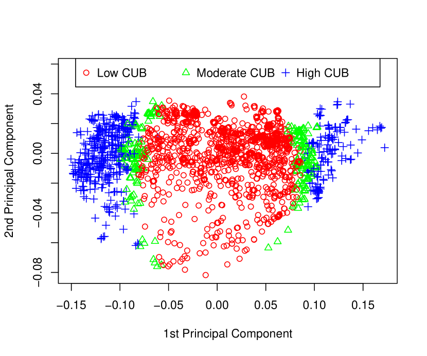
Figure 3: Plot of the first two principal components of the codon distributions of 2535 bacterial chromosomes.

Next, we plotted the first two principal components of the codon distributions, indicating to which group each chromosome belongs. The most significant feature of this plot (see Fig. 3) is that the plot is roughly broken into vertical bands according to membership in the ‘low CUB’,  moderate CUB’or ‘high CUB’ group. Thus, the first principal component captures substantial information concerning CUB in the chromosome. We believe that this may be the first time that this characteristic of the first principal component has been demonstrated at the chromosome level. At present, we have no satisfactory biological explanation for the division of bacterial chromosomes into three groups based on CUB.

References

- Azuma (1967) K. Azuma. Weighted sums of certain dependent random variables. Tôhoku Math.J., 19(3):357–367, 1967. doi: 10.2748/tmj/1178243286.
- Banerjeee et al. (2005) T. Banerjeee, S.K. Gupta, and T.C. Ghosh. Towards a resolution on the inherent methodological weakness of the “effective number of codons used by a gene”. Biochem. Biophys. Res. Commun., 330:1015–1018, 2005.
- Bertoin (2006) J. Bertoin. Random fragmentation and coagulation processesCambridge, volume 102 of Studies in Advanced Mathematics. Cambridge University Press, Cambridge, 2006.
- Comeron and Aguade (1998) J.M. Comeron and M. Aguade. An evaluation of measures of synonymous codon usage bias. J. Mol. Evol., 47:268–274, 1998.
- Fox and Erill (2010) J. Fox and I. Erill. Relative codon adaptation: A generic codon bias index for prediction of gene expression. DNA Res., 17(3):185–196, 2010. doi: 10.1093/dnares/dsq012.
- Fuglsang (2006) A. Fuglsang. Estimating the “effective number of codons”: The wright way of determining codon homozygosity leads to superior estimates. Genetics, 172:1301–1307, 2006. doi: 10.1534/genetics.105.049643.
- Gibbs and Su (2002) A. Gibbs and F. Su. On choosing and bounding probability metrics. Internat. Stadist. Rev., 70(3):419–435, 2002.
- Hoeffding (1963) W. Hoeffding. Probability inequalities for sums of bounded random variables. J. Amer. Stat. Assoc., 58(301):13–30, 1963.
- Karlin et al. (2001) S. Karlin, J. Mrázek, A. Campbell, and D. Kaiser. Characterizations of highly expressed genes of four fast-growing bacteria. J. Bacteriol., 183(17):5025–5040, 2001. doi: 10.1128/JB.183.17.5025-5040 J. Bacteriol. September 2001 vol. 183 no. 17 5025-5040.
- Sharp and Li (1987) P.M. Sharp and W.-H. Li. The codon adaptation index—a measure of directional synonymous codon usage bias and its potential applications. Nucleic Acids Res., 15:1281–1295, 1987.
- Waterman (1995) M. Waterman. Introduction to Computational Biology. Chapman and Hall, London, 1995.
- Wright (1990) F. Wright. The “effective number of codons” used in a gene. Gene, 87:23–29, 1990.