Dynamo saturation in direct simulations of the multi-phase turbulent interstellar medium

Abstract

The ordered magnetic field observed via polarised synchrotron emission in nearby disc galaxies can be explained by a mean-field dynamo operating in the diffuse interstellar medium (ISM). Additionally, vertical-flux initial conditions are potentially able to influence this dynamo via the occurrence of the magnetorotational instability (MRI). We aim to study the influence of various initial field configurations on the saturated state of the mean-field dynamo. This is motivated by the observation that different saturation behaviour was previously obtained for different supernova rates. We perform direct numerical simulations (DNS) of three-dimensional local boxes of the vertically stratified, turbulent interstellar medium, employing shearing-periodic boundary conditions horizontally. Unlike in our previous work, we also impose a vertical seed magnetic field. We run the simulations until the growth of the magnetic energy becomes negligible. We furthermore perform simulations of equivalent 1D dynamo models, with an algebraic quenching mechanism for the dynamo coefficients. We compare the saturation of the magnetic field in the DNS with the algebraic quenching of a mean-field dynamo. The final magnetic field strength found in the direct simulation is in excellent agreement with a quenched $\alpha\Omega$ dynamo. For supernova rates representative of the Milky Way, field losses via a Galactic wind are likely responsible for saturation. We conclude that the relative strength of the turbulent and regular magnetic fields in spiral galaxies may depend on the galaxy’s star formation rate. We propose that a mean field approach with algebraic quenching may serve as a simple sub-grid scale model for galaxy evolution simulations including a prescribed feedback from magnetic fields.

1 Introduction

Magnetic fields in galaxies show coherent structures over kilo-parsec scales (Beck & Wielebinski, 2013; Fletcher, 2010). The magnetic energy is comparable to the turbulent energy of the diffuse interstellar medium (ISM). The action of a mean-field dynamo is likely the main process for large-scale field generation (Parker, 1971; Beck et al., 1996; Shukurov, 2005; Brandenburg & Subramanian, 2005). Although simple heuristic mean-field models can already explain many observational facts, as for instance, a dominant axisymmetric mode in most of the galaxies, the details of the amplification process in the multi-phase ISM have remained hidden. By means of direct numerical simulations of the turbulent ISM, Gressel et al. (2008a) demonstrated the possibility of efficient field amplification through the dynamo effect on fast timescales of a few hundred million years. But the non-linear saturation of the magnetic field is still an open issue. Here we proceed with local box simulations of the turbulent ISM under the influence of rotation and shear, and we furthermore run these simulations until the fields become dynamically important. We are particularly interested in the behaviour of the dynamo closure coefficients in this regime, and we attempt to analyse their effect in the process of nonlinear saturation of the large-scale magnetic fields.

Energy injected by supernova (SN) explosions in combination with the thermal instability (Field, 1965; Kritsuk & Norman, 2002) gives rise to a turbulent multi-phase medium (see, e.g., de Avillez & Breitschwerdt, 2005; Breitschwerdt et al., 2012). We furthermore look for an alternative origin of interstellar turbulence, namely driving of turbulent fluctuations via the magnetorotational instability (MRI). This has been proposed as a source of turbulence in the outer parts of galaxies (Sellwood & Balbus, 1999; Dziourkevitch et al., 2004) but may be suppressed by the turbulent diffusion from SNe (Korpi et al., 2010; Gressel et al., 2013b). Exploring this possibility, we hence extend the analysis performed by Gressel et al. (2008a) to the case of a strong net-vertical flux (NVF) for the seed fields. Neglecting the effect of energy input via supernovae, Piontek & Ostriker (2007) have studied in detail the multi-phase ISM with driving via the MRI alone. We accordingly avoid an extensive discussion of the MRI in this paper, and instead focus on the dynamo action produced by the SN driving. We currently also neglect the contribution from cosmic rays (Hanasz et al., 2006, 2009) – we however plan to address this question in the future.

Many other aspects like chemical evolution (Walch et al., 2014) or details of the energy transfer by radiation processes are beyond the scope of the paper. The main goal here is to understand the amplification and the non-linear evolution of the magnetic field in the ISM. Compared to models with turbulence driven by an artificial forcing (e.g. Mee & Brandenburg, 2006), our approach provides more realistic conditions.

This paper is structured as follows: In section 2 we describe the numerical methods and the physical model used to represent a local patch of the turbulent, multi-phase ISM. General results are presented in section 3.1. In section 3.2 we describe the growth of the mean magnetic field and its saturation. We summarise our results and draw conclusions in sections 4 and 5, respectively.

2 Model Specifications and Methods

We solve the non-ideal magnetohydrodynamics (MHD) equations in a local co-rotating box of dimensions $0.8\times 0.8\times 4.2\,\rm kpc^{3}$, where $x$ corresponds to the radial, $y$ to the azimuthal and $z$ to the vertical direction. A numerical resolution of $96\times 96\times 512$ grid cells is used (grid size $\sim 8.3\,\rm pc$). We use NIRVANA MHD fluid code by Ziegler (2004) for our simulations. The set of equations we have used is described below (suppressing explicit factors of the constant permeability $\mu_{0}$, and with all symbols having their usual meanings):

$$\frac{\partial\rho}{\partial t} = -\nabla\cdot\left(\rho\mathbf{u}\right)\,,$$

$$\frac{\partial\left(\rho\mathbf{u}\right)}{\partial t} = -\nabla\cdot\left(\rho\mathbf{uu}+\mathrm{p}^{\star}-\mathbf{BB}\right)-2\rho\ \Omega\ \hat{z}\times\mathbf{u}$$

$$+2\rho\ \Omega^{2}qx\ \hat{x}+\rho\mathrm{g}\ \hat{z}+\nabla\cdot\tau\,,$$

$$\frac{\partial e}{\partial t} = -\nabla\cdot\left((e+\mathrm{p}^{\star})\,\mathbf{u}-\left(\mathbf{u}\!\cdot\!\mathbf{B}\right)\mathbf{B}\right)+2\rho\ \Omega^{2}qx\ \hat{x}\cdot\mathbf{u}$$

$$+\rho\mathrm{g}\ \hat{z}\cdot\mathbf{u}+\nabla\cdot\left[\tau\mathbf{u}+\eta_{\rm m}\,\mathbf{B}\times\left(\nabla\times\mathbf{B}\right)\right]$$

$$+\nabla\cdot(\kappa\nabla\mathrm{T})-\rho^{2}\Lambda\left(\mathrm{T}\right)+\Gamma_{\rm SN}+\rho\ \Gamma\left(z\right)\,,$$

$$\frac{\partial\mathbf{B}}{\partial t} = \nabla\times\left(\mathbf{u}\times\mathbf{B}-\eta_{\rm m}\nabla\times\mathbf{B}\right)\,,$$ (1)

where the total pressure $\mathrm{p}^{\star}\equiv\mathrm{p}+\mathbf{B}^{2}/2$, and assuming an adiabatic equation of state, $\mathrm{p}=\left(\gamma-1\right)\ \epsilon$, with $\gamma=5/3$, as appropriate for an ideal gas. Employing a total energy formalism, the thermal energy density, $\epsilon$, is computed from the total energy density (denoted by $e$) as,

$$\epsilon = e-\frac{\rho\mathbf{u}^{2}}{2}-\frac{\mathbf{B}^{2}}{2}\,,$$ (2)

and the viscous stress tensor is given by

$$\tau = \tilde{\nu}_{\rm m}\,\left(\nabla\mathbf{u}+(\nabla\mathbf{u})^{\top}-\frac{2}{3}\,(\nabla\cdot\mathbf{u})\right)\,,$$ (3)

where $\tilde{\nu}_{\rm m}$ represents the (molecular) dynamic viscosity coefficient, which is scaled with the density. We use a constant kinematic viscosity $\nu_{\rm m}=0.5\times 10^{25}\,{\rm cm^{2}s^{-1}}$, and a microscopic diffusivity of $\eta_{\rm m}=2\times 10^{24}\,{\rm cm^{2}s^{-1}}$ such that the magnetic Prandtl number ${\rm Pm}\equiv\nu_{\rm m}/\eta_{\rm m}=2.5$ is somewhat larger than unity – reflecting as good as feasible the fact that ${\rm Pm}\gg 1$ under typical ISM conditions.

The heat conduction term, $\nabla\cdot(\kappa\nabla\mathrm{T})$ with a conductivity coefficient, $\kappa$, equivalent of a constant thermal diffusivity, is included mainly for numerical reasons (see discussion in Gressel, 2009). The various other energy source and sink terms, as well as momentum source terms, are described in the following sections.

2.1 Supernova driving and thermodynamics

In our simulations, turbulence is driven by supernova explosions (representing both type I and type II SNe), that are modelled via localised injections of thermal energy. The vertical distributions of the SN explosions are Gaussian with half widths of $325\,\rm pc$ and $\sim 90\,\rm pc$ for type I/II SNe, respectively. The latter value is only approximate, since, to avoid an artificial vertical dispersion of the disc (Gressel et al., 2008b), we use the density profile $\bar{\rho}(z)$ to compute a cumulative distribution function, $\Phi_{\rm II}(z)$ via

$$\Phi_{\rm II}(z)\equiv\frac{L_{x}\,L_{y}}{M}\int_{-L_{z}/2}^{z}\bar{\rho}(z^{\prime})\,{\rm d}z^{\prime}\,,$$ (4)

where $L_{x}$, $L_{y}$ and $L_{z}$ are the $x$, $y$ and $z$ dimensions of the computational domain,respectively. We then map an equally distributed random number $r\in[0,1]$ via the inverse function, $z=\Phi_{\rm II}^{-1}(r)$, to obtain a vertical distribution of type II SNe that follows the average mass density profile. The reference Galactic supernova rates for type I and II are $\sigma_{\rm I}=4\,\rm Myr^{-1}\,\rm kpc^{-2}$ and $\sigma_{\rm II}=30\,\rm Myr^{-1}\,\rm kpc^{-2}$, respectively, and associated energies are $10^{51}$ and $1.14\times 10^{51}\,\rm erg$. We furthermore mimic the effect of spatial clustering for type II SNe, which are known to occur in associations of massive stars. To facilitate such a clustering, we resort to a very crude prescription (Korpi et al., 1999): We first randomly chose the vertical position of the explosion site according to Eq. (4), and then determine random coordinates in the horizontal plane. If the mass density at the chosen explosion site exceeds the average mass density in that vertical slice, we add an explosion, otherwise we chose a new random position in $(x,y)$ but keeping the $z$ coordinate, until the criterion is met. We omit this effect for type I SN explosions.

A vertical profile of mass density with midplane value of $10^{-24}\,\rm g\,\rm cm^{-3}$ (equivalent to $1\,\rm cm^{-3}$) is used as an initial condition for the ISM density. The optically thin radiative cooling function is approximated by a piecewise power law as, $\Lambda(\mathrm{T})=\Lambda_{i}\ {\mathrm{T}}^{\beta_{i}}$, ( with ${\mathrm{T}}_{i}\leq\mathrm{T}\leq\mathrm{T}_{i+1}$). To capture the thermodynamics of the thermally unstable low- temperature range, we implement the equilibrium pressure curve similar to Gazol et al. (2001) for $T<10^{5}\,\rm K$, which reproduces a well separated multi-phase ISM structure in rough agreement with the observed morphology. While choosing a piecewise-power-law approximation for the cooling function, we neglect the detailed non-equilibrium chemistry that will affect the cooling processes at high densities. This is reasonably justified because we are primarily interested in the dynamical aspects of the ISM at comparatively large scales and moderately high densities. Values of $\Lambda_{i}$ and $\beta_{i}$ are chosen in such a way that the temperature range between $141\,\rm K$ and $6102\,\rm K$ is prone to the thermal instability. Detailed discussion and corresponding fitting parameters ($\Lambda_{i}$ and $\beta_{i}$) for the cooling function are given in the section 2.1 of Sánchez-Salcedo et al. (2002). For the temperature $T>10^{-5}\,\rm K$, we use the cooling functions corresponding to the ISM in collisional ionisation equilibrium, similar to Slyz et al. (2005) (values of corresponding $\Lambda_{i}$ and $\beta_{i}$ are listed therein). Gressel (2010) found that the presence of a thermally unstable branch in the cooling function only has a moderate influence on the large-scale dynamo.

Inverting the neutral $p(\rho)$ relation, this provides us with a natural choice for initial pressure profile, $p(z)$, simultaneously satisfying hydrostatic equilibrium and radiative energy balance (and leading to a slight temperature variation in the vertical direction).

2.2 Differential rotation and gravity

In our local model, the background shear originating from the differential galactic rotation is expressed in terms of the shear parameter $q\equiv\mathrm{d}\ln\Omega/\mathrm{d}\ln R$, where $\mathrm{R}$ is the radius in a cylindrical coordinate system with its origin at the galactic centre. With this definition, $q=-1$ corresponds to a flat rotation curve. We use initial conditions (midplane density and SN rate) corresponding to the solar orbit ($\mathrm{R}\simeq 8.5\,\rm kpc$) for all our models. Because of the differentially rotating flow, we use shearing periodic boundary conditions (Gressel & Ziegler, 2007) at the $x$ (radial) boundaries, whereas at the $y$ (azimuthal) and $z$ (vertical) boundaries, we use periodic and outflow boundary conditions, respectively. A vertical profile for acceleration due to gravity is chosen from Gilmore et al. (1989), that is

$$\mathrm{g}(z)=\frac{-a_{1}\ z}{\sqrt{z^{2}-{z_{0}}^{2}}}-a_{2}\ z\,,$$ (5)

with $a_{1}=1.42\times 10^{-3}\,\rm kpc\,\rm Myr^{-2}$, $a_{2}=5.49\times 10^{-4}\,\rm Myr^{-2}$ and $z_{0}=180\,\rm pc$ – with which we tacitly neglect the effects of self gravity (which would presumably only affect the ISM composition in the dense cold part).

2.3 Description of studied models

In the first part of this analysis, we aim to study the effects of the initial magnetic field configuration on the dynamo. We choose three basic types of models, all with a supernova rate of $25\%$ in units of the average rate in the Milky Way $\sigma_{0}$, and where we keep the ratio of $\sigma_{\rm I}$ and $\sigma_{\rm II}$ fixed. The different models are characterised by

1. weak vertical field ($0.001\,\mu\rm G$),
   with and without vertical flux (models ‘Q’ and ‘QZ’).

2. strong vertical field ($0.1\,\mu\rm G$),
   with and without vertical flux (‘QS’ and ‘QSZ’).

3. weak azimuthal field ($0.001\,\mu\rm G$),
   without vertical flux (model ‘AR’).

The description of the nomenclature (Q, QZ etc.) is given in Table 1 as well. It should be noted that the vertical flux of magnetic field in our box is conserved due to the periodic boundaries in the ‘${xy}$’ plane. For reference, we also simulate a model with a zero net flux. A low SN rate together with a vertical flux magnetic field is chosen to include better the possible effects of MRI, which may be suppressed otherwise by a too strong turbulent diffusivity (see e.g. Gressel et al., 2013b). To study the effect of SN driving on dynamo action and ISM composition in general, we simulate two models, with the same initial condition as Q, except we vary SN rates in this case. We call these models H and F, indicative of “half” (H) and “full” (F) supernova rate compared with the galactic SN rate $\sigma_{0}$. Assuming some kind of relation between column density and star formation rate, in reality, however, the SN rate does likely not vary without changing the mass density profile. Nevertheless it is worthwhile to establish how the dynamo process depends on the main driver for ISM turbulence. In the second part, we wish to study the effects of magnetic field and SN rate on the vertical structure.

Table 1: Model parameters for the simulations with vertical ($\rm B_{v}$) and in-plane ($\rm B_{t}$) initial fields. SN rates are in terms of the rate corresponding to the Milky Way, $\sigma_{0}\equiv(\sigma_{I}^{-1}+\sigma_{II}^{-1})^{-1}$. The last column gives the physical time the models have been evolved for.

	$\rm B_{v}$	Flux	$\rm B_{t}$	SN Rate	Time
	$[\,\mu\rm G]$	$[\,\mu\rm G\,\rm kpc^{-2}]$	$[\,\mu\rm G]$	$[\sigma_{0}]$	[ Gyr]
F	0.001	0.0064	0	1.00	1.40
H	0.001	0.0064	0	0.50	1.40
Q	0.001	0.0064	0	0.25	2.08
QZ	0.001	0	0	0.25	1.25
QS	0.1	0.064	0	0.25	1.60
QSZ	0.1	0	0	0.25	1.08
AR	0	0	0.001	0.25	1.50

3 Results

Starting from the initial model, which mostly consists of the warm ionised and transition ISM phases ($5000\,\rm K$ to $10^{5.5}\,\rm K$), the system evolves into a multi-phase turbulent state, that becomes stationary in total thermal ($E_{\rm th}$) and kinetic energy ($E_{\rm kin}$) within the first $20$ to $50\,\rm Myr$. The stationary value of turbulent kinetic energy $E_{\rm kin}$ (not including the kinetic energy of the shear flow) has an approximate dependence, $E_{\rm kin}\sim\sigma^{0.8\pm 0.04}$ on the SN rate $\sigma$. In contrast, $E_{\rm th}$ scales with $\sigma$ as $E_{\rm th}\sim\sigma^{0.5\pm 0.05}$. The vertical profile of the average density $\bar{\rho}(z)$ (that is, averaged over the ${xy}$ plane), also evolves to a steady state within the first $20$ to $50\,\rm Myr$. With a quasi-stationary kinematic background state established, we can now look into the temporal evolution of the magnetic energy density.

3.1 General evolution

The initially Gaussian density profile (with an approximate scale height $\simeq 325\,\rm kpc$) evolves due to the influence of the developing turbulence, that adds a dynamical component to the vertical pressure support. The resulting density profile shows a distinctive thin disc (with $\left|z\right|<0.2\,\rm kpc$ which is unaffected by the SN rate), thick disc (within the range of $0.2<\left|z\right|<1\,\rm kpc$) and a halo component (above $1\,\rm kpc$). Accordingly, the best fit for this function is defined via a superposition of three exponential components, that is,

$$\rho(z)\,\simeq\,\sum_{i=0}^{2}\;\rho_{i}\ \mathrm{exp}\left(\frac{-|\,z\,|}{r_{i}}\right)\,.$$ (6)

Fitting coefficients $\rho_{i}$ and $r_{i}$ are listed in the Table 2 for the three runs Q, H, and F. Scale heights in the halo (that is, $r_{1}$ and $r_{2}$) are found to increase with the SN rate (with a dependence $\sim\sigma^{0.4}$), while $r_{0}$ does not appear to depend on $\sigma$. The equilibrium value of the midplane density, $\rho_{0}$, of this component decreases slightly with increasing SN rate. This is initial distribution does not change much under the influence of the magnetic field.

Table 2: Fitting coefficients for the $\bar{\rho}(z)$ profiles ($\rho_{i}$ and $r_{i}$).

Model	Q	H	F
$\rho_{0}$ $[\,\rm cm^{-3}]$	$0.6\pm 0.1$	$0.5\pm 0.1$	$0.3\pm 0.1$
$r_{0}$ $[\,\rm kpc]$	$0.11\pm 0.04$	$0.12\pm 0.05$	$0.12\pm 0.05$
$\rho_{1}$ $[\,\rm cm^{-3}]$	$0.1\pm 0.03$	$0.1\pm 0.05$	$0.1\pm 0.05$
$r_{1}$ $[\,\rm kpc]$	$0.25\pm 0.04$	$0.35\pm 0.08$	$0.42\pm 0.1$
$\rho_{2}$ $[\,\rm cm^{-3}]$	$0.01\pm 0.002$	$0.01\pm 0.003$	$0.01\pm 0.005$
$r_{2}$ $[\,\rm kpc]$	$0.7\pm 0.3$	$0.9\pm 0.3$	$1.2\pm 0.5$

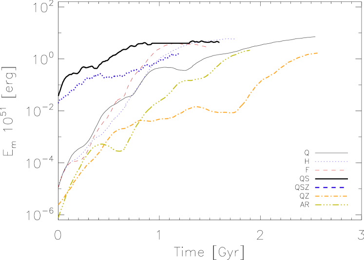
Figure 1: Evolution of the total magnetic energy for the various studied models.

After this initial phase of roughly $50\,\rm Myr$, the total magnetic energy, $E_{\rm m}$, grows exponentially. This happens with almost the same e-folding time, of about $100\,\rm Myr$, irrespective of SN rate for several hundred million years. This is shown in Fig. 1, where we plot the time evolution of the magnetic energy. Quite interestingly, the growth rate is slightly slower for the models with higher initial field strengths (models QS, and QSZ), probably due to non-linear quenching effects already becoming relevant.

The fast growth phase lasts until the total magnetic energies $E_{\rm m}$ are 6.6, 7.8 and $10.5\times 10^{50}{\,\rm erg}$ or the ratios to the kinetic energies $E_{\rm m}/E_{\rm kin}$ are $0.25$, $0.14$ and $0.1$, in the three models with increasing supernova rate. This state is reached after $1.2,1.0$ and $0.8\,\rm Gyr$ for model Q, H, and F, respectively. Afterwards, the growth rate continuously decreases for models Q and H, but $E_{\rm m}$ keeps growing – consistent with the derived algebraic quenching for the appropriate mean-field model (cf. section 3.2.1). For model F, the growth stops after about $1\,\rm Gyr$. We shall refer to this phase as the dynamical state, in contrast to the initial kinematic growth phase.

Table 3: Temperature components of the ISM and average pressures at the mid plane $z=0$ for model Q

	T	$\rho$	$\langle{P_{\rm th}}\rangle$	$\langle{P_{\rm kin}}\rangle$
	$[\,\rm K]$	$[\,\rm cm^{-3}]$	$[10^{-14}\ \mathrm{Pa}]$	$[10^{-14}\ \mathrm{Pa}]$
Cold	$0-200$	$10$	$2$	$4$
Cool	$200-5000$	$1$	$5$	$1.5$
Warm	$5000-10^{4.4}$	$0.1$	$6$	$1.5$
Trans	$10^{4.4}-10^{5.5}$	$5\times 10^{-3}$	$10$	$15$
Hot	$>10^{5.5}$	$5\times 10^{-5}$	$100$	$50$

Table 4: Composition of each ISM component at the end of the kinematic phase, i.e. at $1.2,1.0$ and $0.9\,\rm Gyr$ for Q, H and F respectively. Energy fractions are calculated within the inner thin disc of $|z|<0.5\,\rm kpc$, but Volume filling fractions (VFF) and mass filling fractions (MFF) are calculated for the entire box.

	Cold	Cool	Warm	Trans	Hot	Total
model Q
$E_{\rm m}/E_{\rm kin}$	1.0	1.2	2.3	0.6	0.03	1.6
$E_{\rm m}/E_{\rm th}$	2.0	0.8	1.0	0.6	0.01	0.8
$E_{\rm kin}/E_{\rm th}$	1.7	0.3	0.4	1.1	0.4	0.5
VFF (%)	0.02	1.9	20	55	23	100
MFF (%)	3	28	62	6.5	0.25	100
model H
$E_{\rm m}/E_{\rm kin}$	0.5	1.0	1.2	0.5	0.03	0.8
$E_{\rm m}/E_{\rm th}$	1.8	0.6	0.9	0.5	0.02	0.6
$E_{\rm kin}/E_{\rm th}$	3.3	0.6	0.6	1.1	0.4	0.7
VFF (%)	0.01	1.7	18	50	30	100
MFF (%)	2	26	60	11	0.6	100
model F
$E_{\rm m}/E_{\rm kin}$	0.1	0.5	0.7	0.35	0.04	0.2
$E_{\rm m}/E_{\rm th}$	0.7	0.7	0.8	0.3	0.02	0.2
$E_{\rm kin}/E_{\rm th}$	8.3	1.0	1.0	1.1	0.4	0.8
VFF (%)	0.006	1.5	14	45	40	100
MFF (%)	1.6	22	55	21	1.4	100

To illustrate the relative distribution of the different energy forms with respect to the various ISM phases, we define five different temperature ranges in Table 3 and give the distribution of magnetic, thermal and kinetic energy fractions within these ISM phases in Table 4, along with the corresponding volume filling fractions (VFF) and mass filling fractions (MFF).

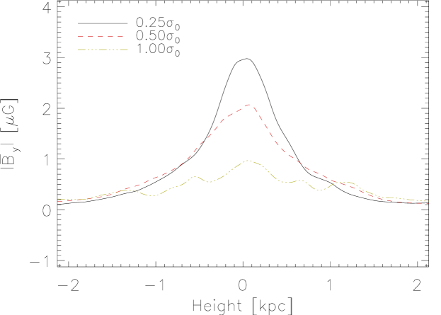
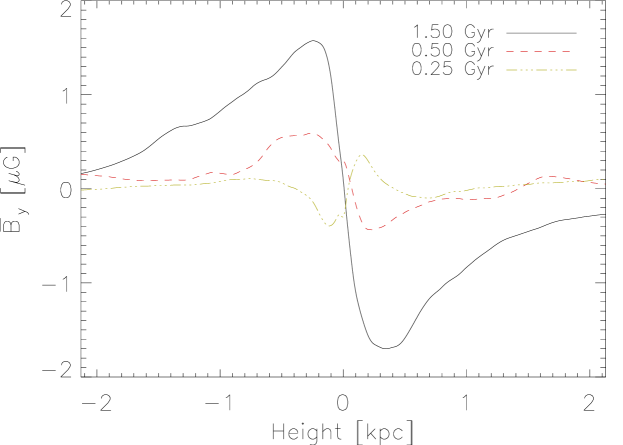
(a)        (b)
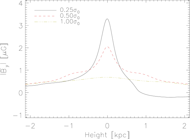
(c)        (d)

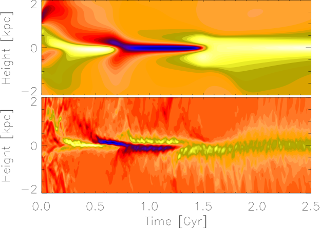
Figure 2: Upper-left: Vertical profiles (from DNS) of the mean azimuthal magnetic field. Lines are for model Q (black; solid), for model H (red; dashed) and for model F (green; dot-dashed).   Upper-right: Vertical profiles of the final mean magnetic field from a 1D dynamo model (see section  3.2.2).   Lower-left: Vertical profiles of the mean magnetic field at different times, for the strong net-flux model, QS, at low supernova rate.   Lower-right: Space-time-evolution of vertical profiles of the azimuthal magnetic field for model Q, color code indicates the strength of magnetic field normalised with the square root of magnetic energy $E_{m}(t)$, which is to compensate for the exponential growth in time and make the vertical mode structure visible. The two panels compare the evolution seen in the simple 1D dynamo model (upper panel, see section  3.2.2 for details) with the actual evolution in the DNS (lower panel).

3.1.1 Mean magnetic field

By averaging over horizontal planes, we split physical quantities like the total magnetic field, $\mathbf{B}$, into its mean part,

$$\bar{\mathbf{B}}(z)=\frac{1}{L_{x}L_{y}}\int\int{\mathbf{B}}\ {\rm d}x\,{\rm d}y\,,$$ (7)

and fluctuating part, $\mathbf{b^{\prime}}=\mathbf{B}-\bar{\mathbf{B}}(z)$. Due to the periodic and shearing periodic boundary conditions in the $y$ and $x$ directions respectively, the vertical ($z$) component of the magnetic flux remains unchanged throughout the evolution (subject to the solenoidal constraint). Moreover, we find that the $x$ component of $\bar{\mathbf{B}}$ remains 3 to 5 times smaller than the $y$ component. For the purpose of brevity, we only present the azimuthal component in the plots. The vertical profile of $\bar{B}_{y}$ (and of $\bar{B}_{x}$) goes through several reversals and parity changes as it evolves in time, (see the lower right panel of Fig. 2). Finally, it achieves a steady-state S mode (i.e, symmetric with respect to the midplane) in all models with weak (or zero) initial vertical flux (models Q, H, F, QZ, QSZ and AR).

The vertical shape found in DNS and a 1D mean-field model (cf. section 3.2.2) are shown in panels (a) and (b) of Fig. 2 for models Q, H, and F, respectively. Vertical profiles at different times are shown for model QS in panel (c) of the same figure, along with the evolution of the mean azimuthal field for model Q, which is shown in panel (d). At late times, we obtain fits for these $\bar{B}_{y}(z)$ profiles, again applying a superposition of exponential functions with different scale heights, $h_{i}$, within the disc ($-0.8$ to $0.8\,\rm kpc$), and within the halo (above $0.8\,\rm kpc$).

$$\bar{B}_{y}(z)\simeq\sum_{i=0}^{1}B_{i}\ \mathrm{exp}\left(-\frac{|\,z\,|}{h_{i}}\right),$$ (8)

values of the fitting coefficients ($B_{i}$ and $h_{i}$) are listed in Table 5. We generally find the scale heights to increase with increasing SN rate, reflecting the vertical equilibration process with the additional kinetic pressure from the SNe.

Table 5: Fitting coefficients ($B_{i}$ and $h_{i}$) for the mean (azimuthal) magnetic field $\bar{B}_{y}(z)$.

	$B_{0}$	$h_{0}$	$B_{1}$	$h_{1}$	$v_{\rm A}^{\prime}(z\!=\!0)$
	$[\,\mu\rm G]$	$[\,\rm kpc]$	$[\,\mu\rm G]$	$[\,\rm kpc]$	$[\,\rm km\,s^{-1}]$
Q	$1.8\pm 0.2$	$0.5\pm 0.1$	$0.2\pm 0.1$	$1.2\pm 0.4$	$10\pm 0.5$
H	$1.5\pm 0.2$	$0.6\pm 0.2$	$0.3\pm 0.1$	$2.1\pm 0.8$	$14\pm 0.5$
F	$0.7\pm 0.3$	$0.8\pm 0.2$	$0.4\pm 0.2$	$3.6\pm 1.4$	$18\pm 0.5$

Notes: The scale heights for the rms $B(z)$ and mean azimuthal field, $\bar{B}_{y}(z)$ are nearly the same, consistent with a constant ratio of rms to mean field. Midplane Alfvén velocities, $v_{\rm A}^{\prime}(z=0)$, are stated at the end of kinematic phase, and roughly scale with the SN rate, $\sigma$, via a power law $v_{\rm A}^{\prime}\sim\sigma^{0.4}$.

The midplane field strength, however, scales inversely with respect to the SN rate (see the upper-left panel in Fig. 2). Moreover, flat regions in the energy evolution curve, shown in Fig. 1, correspond to a flip in the field direction, and these are also related to parity changes. The model with high initial flux (QS which shows a strong ‘A’ mode initially) remains finally an ‘A’ mode but with the same ratio of $E_{\rm m}$ and $E_{\rm kin}$ as model Q. This is probably a consequence of our boundary conditions, which conserve the vertical magnetic flux. Initial growth times for QS and QSZ models are higher compared with the weak flux models, which will be explained in the next section.

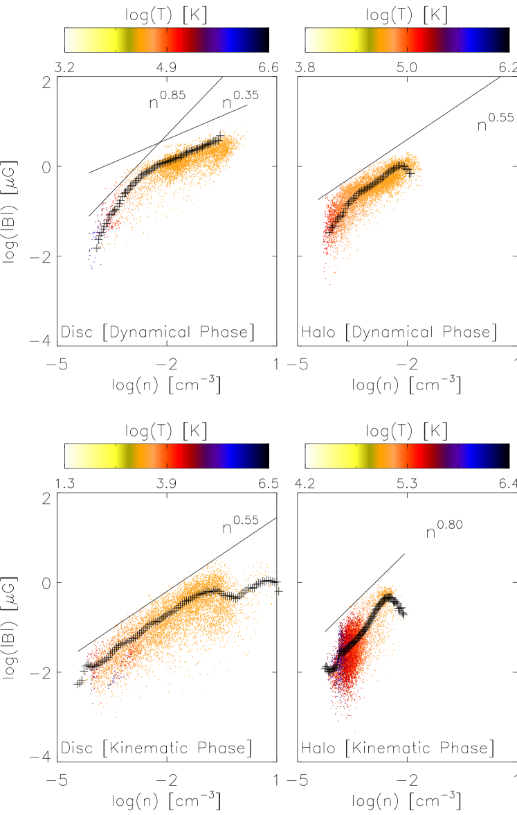
Figure 3: Typical distribution of the total magnetic field strength as a function of the mass density for model Q. The lower and upper rows compare the $B$-$\rho$ relation at early and late times, respectively, whereas the left and right columns compare the disc region $|z|<0.5\,\rm kpc$ with the halo $|z|>0.5\,\rm kpc$. The colour coding indicates the temperature in ${\rm K}$ as shown in the colour bar above each panel. ‘$+$’ signs indicate the average value of total magnetic field for the corresponding density. Black straight lines in each panel show the best fit for the particular branch of the distribution, with power law exponents as shown.

3.1.2 Fluctuating fields

Root mean squared (rms) magnetic field profiles are defined by

$$B(z)=\left[\frac{1}{L_{x}L_{y}}\int\int{\left(\mathbf{B}\!\cdot\!\mathbf{B}\right)\ {\rm d}x\,{\rm d}y}\right]^{1/2}\,,$$ (9)

which are also best fitted with a function as the one in Eq. (8), and scale heights ($h_{i}$) which are equivalent to the ones, that are listed in Table 5 for the mean field. We observe that the $B(z)$ profiles become wider with SN rate, that is, the coefficients $h_{i}$ are directly proportional to $\sigma$. $B(z)$ have the same scale heights as those of the mean fields, $\bar{B}_{y}(z)$, and midplane field strengths are about $3\,\mu\rm G$ (at the end of kinematic phase) for all the models. By virtue of field-line stretching and transverse compression, amplification of $\mathbf{B}$ occurs in such a way that there exists a statistical correlation between $B$ and $\rho$. To a first approximation, this can be described as $B\propto\rho^{a}$, with a certain exponent $a$, and where, for instance, $a=2/3$ would correspond to amplification via compression in the two directions perpendicular to the field line, and $a=1/2$ would correspond to energy equipartition between magnetic and kinetic energy (assuming a constant velocity dispersion). From a scatter plot of $B$ versus $\rho$, we find that $B$ scales with a different power law exponent within the disc and in the halo. The coefficient is furthermore seen to have a dependence on the field strength and SN rate. This is represented in Fig. 3, in which we have plotted the typical $B$-$\rho$ distribution during the kinematic as well as in the dynamical phase for model Q. First we consider only the disc midplane region ($|z|<0.5\,\rm kpc$) during the kinematic phase. For this particular regime, typical values of the exponent are $a\sim 0.5$. Later during the dynamical phase, we obtain $a\sim 0.3$ for the dense ISM, that is for $n>0.01\,\rm cm^{-3}$, whereas for the lighter ISM we obtain $a\sim 1$. The flattening of the relation in the dense part may be explained by the increasing dominance of the mean field over the fluctuating field. For model F, the effect of a flattening of the relation is least pronounced, and we find $a\sim 0.4$ at late times (not shown) – possibly because the quenching of the dynamo coefficients is smaller compared with models Q and H (see Section 3.2.2).

In order to explain the comparatively steeper $B$-$\rho$ correlation in the low-density ISM, we consider the scenario of flux freezing. That is the regular field lines stretch out due to radially expanding SN remnants (in the disc), and only negligible magnetic fields remain inside the expanding shell (that is, in the low density ISM). Now we consider the disc halo ($|z|>0.5\,\rm kpc$). For this region $B$ scales as $\sim\rho^{0.8}$ during the initial kinematic phase (similar to compressional amplification). Later during the dynamical phase the magnetic field density relation becomes again more flat with $a\sim 0.5$.

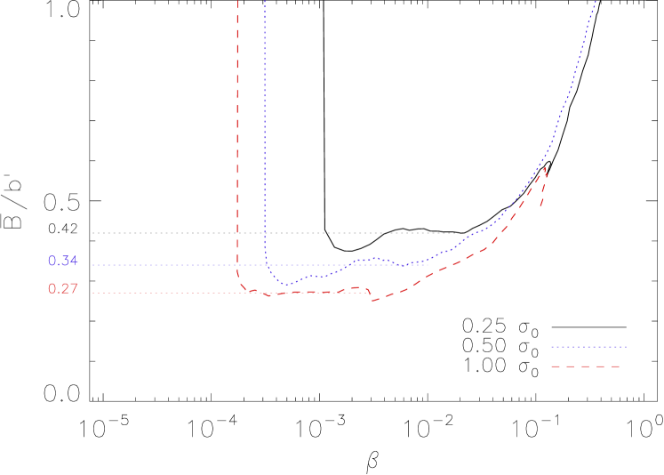
Figure 4: Ratio, $|\overline{\mathbf{B}}|/|\mathbf{b}^{\prime}|$, of the average and turbulent magnetic field strengths versus the relative mean field strength, $\beta$ (formally defined in Eq. (15) in section 3.2.1 below) for model Q, H, and F. Values are calculated in the vertical range $|\,z,|<1\,\rm kpc$. Within this range, we observe regular vertical profiles for the dynamo tensor coefficients. Flat regions satisfy a scaling relation $|\overline{\mathbf{B}}|/|\mathbf{b}^{\prime}|\sim\sigma^{-0.30\pm 0.07}$, as also found by Gressel et al. (2008a).

Fig. 4 shows the evolution of the ratio $|\overline{\mathbf{B}}|/|\mathbf{b}^{\prime}|$ as a function of the relative field strength, $\beta\equiv\bar{B}/B_{\rm eq}$, where $B_{\rm eq}$ represents the field strength where the magnetic energy is in equipartition with the turbulent kinetic energy. The ratio $|\overline{\mathbf{B}}|/|\mathbf{b}^{\prime}|$ remains constant during the kinematic phase (characterised by $\beta\ll 1$), but later in the dynamical phase (with $\beta\simeq 1$) this ratio increases by the increasing importance of the background shear term relative to the turbulence. Typical values of $|\mathbf{b^{\prime}}|$ at the end of the kinematic phase are $\sim 2$ to $4\,\mu\rm G$, with corresponding values of $|\overline{\mathbf{B}}|/|\mathbf{b}^{\prime}|$ approximately $0.3$ to $0.5$. After a short initial decrease, the ratio remains constant during the kinematic growth phase of $E_{\rm m}$. The stationary values of this ratio depend on the SN rate by the relation $|\overline{\mathbf{B}}|/|\mathbf{b}^{\prime}|\sim\sigma^{-0.30\pm 0.07}$, which matches with the observations of Chyży (2008), and which was also previously found in similar simulations without a net-vertical flux (Gressel et al., 2008a). During the dynamical phase, ‘$z$’ profiles of the turbulent field have the same scale heights as that of $\bar{B}_{y}$, suggesting that magnetic fluctuations are likely produced via the mechanism of field-line tangling, that is $\mathrm{b^{\prime}}\sim\tau_{\rm c}l_{\rm d}^{-1}\bar{B}\,u_{\rm rms}$, where $\tau_{\rm c}$, and $l_{\rm d}$ are appropriate turbulent coherence time and diffusion length scales, respectively. We remark that the field-line tangling term, $\nabla\times(\mathbf{u}^{\prime}\times\overline{\mathbf{B}})$ is distinct from the small-scale dynamo term, represented by $\nabla\times(\mathbf{u}^{\prime}\times\mathbf{b}^{\prime})$ in the induction equation for the fluctuating field, and that it transfers magnetic energy from ordered ($\overline{\mathbf{B}}$) to fluctuating ($\mathbf{b}^{\prime}$) fields by “tangling up” the large-scale coherent field. Because, in the regime of supersonic turbulence, the small-scale dynamo possesses a higher critical Reynolds number (Federrath et al., 2011, 2014), field-line tangling may provide an attractive alternative to the classic small-scale dynamo (Kazantsev, 1968; Schober et al., 2012a, b, 2013) in explaining strong fluctuating magnetic fields.

3.1.3 Alfvén velocities

Vertical profiles of the total-field Alfvén velocity are given by the relation

$$v_{\rm A}(z)=\frac{1}{L_{x}L_{y}}\int\int{\frac{|\mathbf{B}|}{\sqrt{\rho}}}\ {\rm d}x\,{\rm d}y\,.$$ (10)

The resulting $v_{\rm A}(z)$ saturates to an inverted-bell-shaped vertical profile for all SN rates. Within the midplane, it scales with $\sigma$ with amplitudes of $10$, $15$ and $18\,\rm km\,s^{-1}$ for models Q, H and F, respectively. Above $\sim 1.0\,\rm kpc$, its amplitude ranges up to $\sim 28\pm 5\,\rm km\,s^{-1}$, irrespective of $\sigma$. Alfvén velocities are typically represented as a ratio of vertical profiles of the rms magnetic field, $B(z)$, and the square root of the average density, that is,

$$v_{\rm A}^{\prime}(z)=\frac{B(z)}{\sqrt{\bar{\rho}}}\,.$$ (11)

Table 5 shows the midplane values of $v_{\rm A}^{\prime}$. These are 10, 14, and $18\,\rm km\,s^{-1}$ for models Q, H, and F, respectively, and as such roughly scale as $\sigma^{0.4}$ in the midplane. The corresponding values in the halo (that is, for $|\,z\,|>1.0\,\rm kpc$) are found to be constant with $\sigma$. During the kinematic phase, Alfvén velocity profiles $v_{\rm A}(z)$ and $v^{\prime}_{\rm A}(z)$ differ by about 25% in the halo (with $v_{\rm A}<v_{\rm A}^{\prime}$), but they are same within the disc. In contrast, in the dynamical phase they match with a good accuracy, except the difference of $\sim-15\%$ within the range of $\pm 0.8$ to $\pm 1.2\,\rm kpc$ ($v^{\prime}_{\rm A}<v_{\rm A}$), potentially indicating the loss of a statistical correlation between density and Alfvén velocity in the dynamical evolution phase.

3.1.4 Mean and fluctuating fluid velocities

Similar to the magnetic field, velocity fields, $\mathbf{u}$, are also split into their mean ($\bar{\mathbf{u}}$) and fluctuating part ($\mathbf{u}^{\prime}=\mathbf{u}-\bar{\mathbf{u}}$). The mean flow velocity, $\bar{\mathbf{u}}$, is defined as

$$\bar{\mathbf{u}}(z)=\frac{1}{L_{x}L_{y}}\int\int{\mathbf{u}}\ {\rm d}x\,{\rm d}y\,.$$ (12)

Since there is no radial (or azimuthal) variation of SN distribution, only the ${\bar{u}}_{z}(z)$ profiles are non-zero, and we find them to be roughly linear in $z$ (see Fig. 5, lower-left, black solid lines). For their overall amplitude, we observe a power law scaling with respect to SN rate as ${\bar{u}}_{z}(z)\sim\sigma^{0.4}$ (also cf. Table 6, below). As a consequence of the vertical density stratification, $\mathbf{u}^{\prime}(z)$ has an inverted-bell-shape profile, (similar to the Alfvén velocity) within the inner disc ($|\,z\,|<0.8\,\rm kpc$), and a constant or decreasing linear profile within the outer halo ($|\,z\,|>0.8$). The resulting M-shaped profile illustrates that, despite the energy input is peaking in the midplane, it is easier to maintain a velocity dispersion at intermediate densities than within the dense Galactic midplane. The maxima of $\mathbf{u}^{\prime}$ (which are situated at $z=\pm 0.8\,\rm kpc$) are 20, 30 and $40\,\rm km\,s^{-1}$ for models Q, H and F, respectively and scale roughly with the SN rate as $\mathbf{u}^{\prime}\sim\sigma^{0.4}$. The midplane values of 6, 11 and 25 $\,\rm km\,s^{-1}$ (for Q, H and F), however, scale as $\sim\sigma^{1.0\pm 0.1}$. In conclusion, we also remark that the width of the inner $\mathbf{u}^{\prime}(z)$ profile becomes broader ($-1.0\,\rm kpc$ to $+1.0\,\rm kpc$) in the dynamical growth phase of $E_{\rm mag}$.

3.2 Growth and saturation of the dynamo

In order to understand the kinematic and dynamic phases of magnetic energy amplification for different SN rates seen in Fig. 1, we employ a mean-field approach based on the $\alpha\Omega$ dynamo framework. A similar model has been used previously to explain the initial amplification of the magnetic energy in the kinematic evolution phase (Gressel, 2010) of the dynamo. For the present analysis, we use the standard mean-field formulation (see, for instance, Rädler, 2007). The approach is based on obtaining a closure for the correlation between the turbulent velocity ${\mathbf{u}}^{\prime}$ and turbulent magnetic field $\mathbf{b}^{\prime}$ – the so-called ‘turbulent electromotive force’, $\mathcal{E}$, which is itself a mean quantity:

$$\mathcal{E}=\overline{\mathbf{u}^{\prime}\times\mathbf{b}^{\prime}}\,.$$ (13)

We adopt a local mean-field formulation in Cartesian geometry, (Brandenburg, 2005), and define the average of the fluid variables ($\mathbf{B}$, $\mathbf{u}$) over the ${xy}$ plane (cf. section 3.1.1 and section 3.1.4). Motivated by the second-order correlation approximation (SOCA), the vertical profile, $\mathcal{E}(z,t)$ is expanded into a linear function of the average magnetic field profile, $\bar{\mathbf{B}}(z,t)$ as

$$\mathcal{E}\,(z,t)=\alpha\,\overline{\mathbf{B}}\,(z,t)-\eta\,\nabla\times\overline{\mathbf{B}}\,(z,t)\,,$$ (14)

where $\alpha$ and $\eta$ are now tensorial quantities referred to as the ‘dynamo coefficients’. Applying the SOCA approximation to isotropic, homogeneous turbulence, one can associate the diagonal elements of the $\alpha$ tensor with kinetic helicity, $\alpha_{xx}=\alpha_{yy}=\alpha_{\rm iso}\sim-\tau_{\rm c}\,\overline{\mathbf{u}^{\prime}\cdot\left(\nabla\times\mathbf{u}^{\prime}\right)}/3$ (note the minus sign). Another important effect known from the realm of this theory, is the turbulent (or diamagnetic) pumping, $\gamma\equiv 0.5\,(\alpha_{xy}-\alpha_{yx})$, which describes the non-advective redistribution of magnetic flux by gradients in turbulent intensity, that is, $\gamma\sim-\tau_{\rm c}/6\,\nabla\mathbf{u}^{\prime 2}$, again from SOCA. The diagonal elements of the $\eta$ tensor are commonly referred to as “eddy” diffusivity, and the SOCA estimate is $\eta\sim\tau_{\rm c}/3\,\mathbf{u}^{\prime 2}$. Note that the quantities $\tau_{\rm c}$ appearing in the preceding expressions are not required to be identical but may differ by factors of order unity among each other.

3.2.1 Quenching of mean-field coefficients

To compute approximate values of $\alpha(z,t)$ and $\eta(z,t)$ tensors from our DNS, we use the test-field approach as described in Brandenburg et al. (2008). To obtain enough independent pieces of information to invert the tensor equation (14), additional passive test fields are evolved parallel to the main simulation run. $\mathcal{E}(z,t)$ is then computed for the associated test-field fluctuations, $\mathbf{b}^{\prime}$, via Eq.  (13), and Eq. (14) is inverted to obtain the tensors $\alpha(z,t)$ and $\eta(z,t)$ as a function of time. A detailed description of this method is beyond the scope of this paper, and we refer the interested reader to appendix B in Gressel (2010).

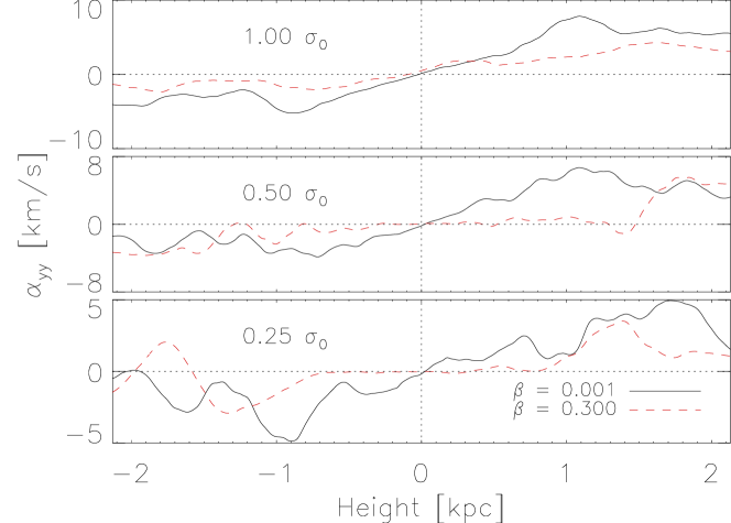
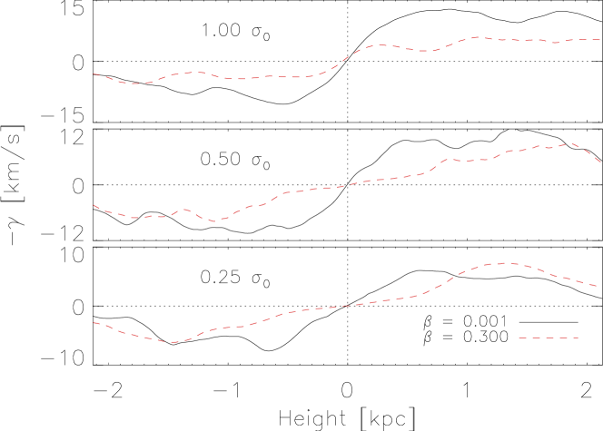
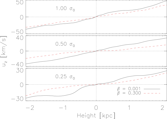
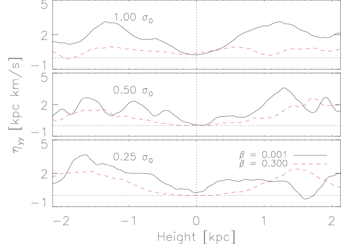
Figure 5: Vertical profiles of the various dynamo coefficients of interest, averaged over $0.2\,\rm Gyr$ in the kinematic phase (solid black lines) and in the dynamic phase (dotted red lines). The three plots of each sub-panel correspond to model F, H, and Q, with diminishing supernova rate, $\sigma=1$, 0.5, and 0.25, respectively. The quantities shown are (top-left to bottom-right): the dynamo effect, $\alpha_{yy}(z)$ (relevant for the $\alpha\Omega$ mechanism), diamagnetic pumping, $\gamma(z)$ (note the negative sign), the mean vertical flow velocity, ${\bar{u}}_{z}(z)$, and the eddy diffusivity, $\eta_{yy}(z)$. The values of the corresponding normalised field strength, $\beta$, defined by Eq. (15), are $10^{-3}$ (kinematic regime) and $0.3$ (quenched regime), respectively.

The black solid lines in Fig. 5 show the $z$ profiles of all dynamo coefficients for three different values of $\sigma$, corresponding to model, F,H, and Q, respectively. We also list, in Tab. 6, the values of $\alpha$ and $\eta$ in the halo for the different values of $\sigma$ in the kinematic phase. The amplitude of the dynamo coefficients is found to scale with the supernova rate as $\sim\sigma^{0.4}$ (see Table 6). In reality, the increase in the SN rate is associated with the increase in density (e.g. Kennicutt, 1998). For the present analysis, however, we do not change these two parameters simultaneously. This is done in order to obtain the explicit dependencies on these variables, which can later be used in parametrisations.

Table 6: Dynamo coefficients (at $z=1\,\rm kpc$), and vertical wind velocity $\bar{u}_{z}$ (at $z=2\,\rm kpc$), both in the kinematic phase. Scaling laws for the respective amplitudes of $\alpha$, $\eta$, $\gamma$, and $\bar{u}_{z}$ are $\sim{\sigma}^{0.4}$.

	$\sigma$	$\alpha_{xx}$	$\alpha_{yy}$	$\gamma$
	$[\sigma_{0}]$	$[\,\rm km\,s^{-1}]$	$[\,\rm km\,s^{-1}]$	$[\,\rm km\,s^{-1}]$
Q	0.25	$3.5\pm 0.8$ [4.0]	$3.8\pm 0.9$ [4.5]	$9.7\pm 2$ [7.6]
H	0.50	$4.6\pm 1.7$ [5.3]	$4.9\pm 2.0$ [6.6]	$12\pm 2$ [9.5]
F	1.00	$6.1\pm 2.0$ [7.0]	$6.6\pm 3.0$ [7.8]	$15\pm 4$ [13.5]
	$\sigma$	$\eta_{xx}$	$\eta_{yy}$	$\mathrm{u_{z}}$
	$[\sigma_{0}]$	$[\,\rm kpc\,\rm km\,s^{-1}]$	$[\,\rm kpc\,\rm km\,s^{-1}]$	$[\,\rm km\,s^{-1}]$
Q	0.25	$1.8\pm 0.5$ [1.5]	$2.6\pm 0.6$ [2.1]	$28\pm 2$ [30]
H	0.50	$2.5\pm 0.8$ [1.9]	$3.3\pm 1.1$ [2.7]	$35\pm 4$ [37]
F	1.00	$3.2\pm 1.5$ [2.5]	$4.4\pm 1.6$ [3.1]	$45\pm 4$ [44]

Notes: Numbers in the squared bracket represent the values of corresponding coefficient, obtained by fitting the data with the Legendre polynomials, which we further use in 1D simulations (cf. section 3.2.2).

The dynamo coefficients are found to be quasi-stationary in time only while the flow structure is uninfluenced by the magnetic field, that is, in the kinematic phase, characterised by $v_{\rm A}\ll u^{\prime}$. In the dynamical phase, the expansion of $\mathcal{E}$ from Eq. (14) is no longer a strict linear function of $\bar{\mathbf{B}}$, but is non-linearly “quenched” (see, e.g., Rädler, 2007). As a consequence, in the most simple case, the amplification of $\bar{\mathbf{B}}$ is expected to slow down if the $\alpha$ effect diminishes more strongly than the turbulent diffusivity, $\eta$.

The quenching of the vertical profiles is qualitatively represented in Fig. 5, where black-solid lines show the initial unquenched profiles, which during the dynamical evolution stage become less steep (as shown by red dashed lines). To describe this effect in a quantitative manner, we here represent the dynamical importance of mean fields by the ratio $\beta$, which describes the relative magnitude of the Alfvén and turbulent rms velocities, that is,

$$\beta=\frac{{\left(\bar{B}_{x}^{2}+\bar{B}_{y}^{2}\right)}^{1/2}}{\sqrt{\rho\,u^{\prime 2}}}\,,$$ (15)

equivalent to the square-root of the ratio of magnetic and kinetic pressure, and where we ignore the contribution from the (fixed) weak vertical mean field. Since the vertical profiles of turbulent kinetic energy and turbulent magnetic fields are Gaussian, the vertical profile of $\beta$ has the same functional form, i.e. $\beta$ in the disc is greater than its halo value by $\sim 20\%$. We note that, when increasing the supernova rate, the vertical profiles of $\beta\left(z\right)$ become flat. For model F, the difference between the disc and halo values of $\beta$ is $\sim 5\%$, while for model Q, the difference becomes as high as $\sim 30$ to $40\%$.

To derive the dependence of dynamo effects on the presence of mean fields, we fit the coefficients by a standard algebraic function of $\beta(z)$ as defined by, eq. (1) in Gressel et al. (2013a). Recently, Chamandy et al. (2014) used a similar approach to demonstrate the saturation of $E_{\rm m}$ in 1D dynamo models. Using the test-field method, we obtain the following quenching relations (Gressel et al., 2013a)

$$\alpha=\frac{\alpha_{\rm k}}{1+27\,\beta^{2}}\,,\quad\eta=\frac{\eta_{\rm k}}{1+6\,\beta}\,,\quad\gamma=\frac{\gamma_{\rm k}}{1+10\,\beta^{2}}\,,$$ (16)

where $\alpha_{\rm k}$, $\eta_{\rm k}$ and $\gamma_{\rm k}$ are the unquenched amplitudes of the dynamo coefficients during the initial kinematic phase, that depend upon the SN rate as $\alpha_{\rm k}=\alpha_{0}\ (\sigma/\sigma_{0})^{0.4}$, $\eta_{\rm k}=\eta_{0}\ (\sigma/\sigma_{0})^{0.4}$, and $\gamma_{\rm k}=\gamma_{0}\ (\sigma/\sigma_{0})^{0.4}$ (see Table 6).

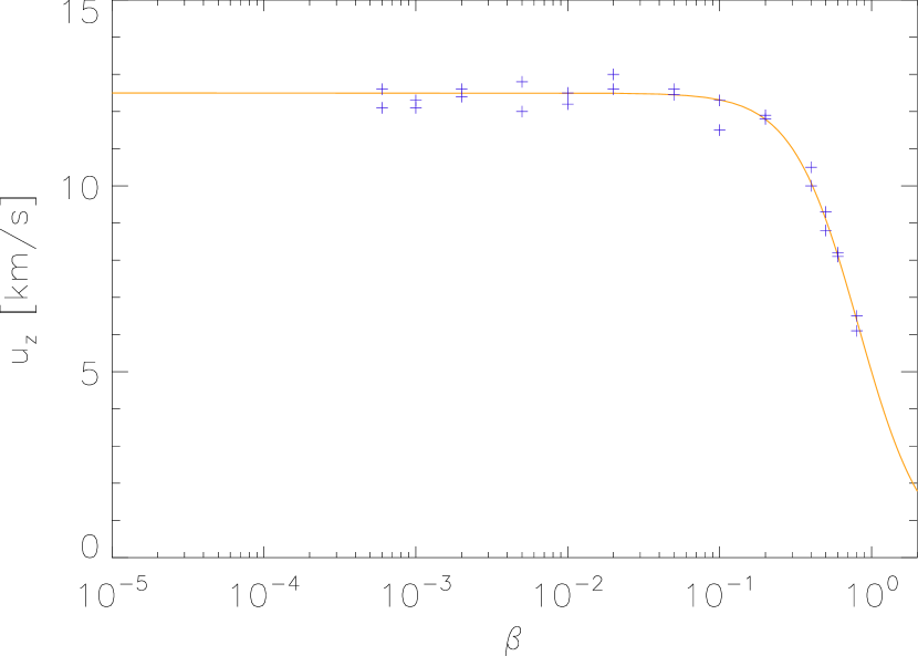
Figure 6: Quenching of the vertical wind with respect to $\beta$, calculated for model Q at a reference height of $z=\pm 0.8\,\rm kpc$, representing the vertical disc region that we find to be affected by the quenching. The resulting relation, $\bar{u}_{z}=\bar{u}_{z\,0}/{(1+1.5\,\beta^{2})}$, means that quenching of the wind sets in at a comparatively higher value of $\beta$ than in relation (16) for $\gamma(z)$. Two ’+’ signs corresponding to the same $\beta$ represent the value of $\bar{u}_{z}$ above and below the midplane

The horizontal components of the mean velocity in our co-rotating frame are negligibly small, so we have to include only the mean vertical velocity $\bar{u}_{z}$ into the dynamo equations. The amplitude of the vertical profile of the mean velocity was found to scale with the supernova rate as $\sigma^{0.4}$, (see Fig. 5 and Tab. 6). In the dynamical phase, the mean velocity profiles furthermore undergo non-linear quenching. We find the best fit for it using our direct simulations data, which has the same algebraic form as for $\gamma(\beta)$. The quenching for model Q and H appears mainly around the midplane, where $\beta$ is maximal. Figure 6 shows the dependence of ${\bar{u}}_{z}$ on $\beta$ at $z=\pm 0.8\,\rm kpc$. This dependence is also reflected in the linear slope of the $\bar{u}_{z}(z)$ profile within approximately $-1\,\rm kpc<z<+1\,\rm kpc$, which is to say that we would obtain a similar $\beta$ dependence if we were to measure this relation at a different reference point within this interval. The obtained quenching of ${\bar{u}}_{z}$ is

$$\bar{u}_{z}=\frac{\bar{u}_{\rm k}}{1+1.5\,\beta^{2}}\,,$$ (17)

where the initial unquenched amplitudes $\bar{u}_{k}$ also scale with the SN rate as $\bar{u}_{k}=\bar{u}_{0}\ (\sigma/\sigma_{0})^{0.4}$ (see Tab. 6).

Above $\sim 1.2\,\rm kpc$, fluctuations in $\bar{u}_{z}(z)$ are comparatively larger, and the estimated error in $\bar{u}_{z}(\beta)$ from Eq. (17) is more than $\pm 40\%$. Equation (17) also enters the mean-field description of the one-dimensional $\alpha\Omega$ dynamo model that we will describe in the following section. The quenching of the wind profiles can be qualitatively seen in the lower-left panel of Fig. 5, and is comparatively weaker than the $\gamma$ quenching – as can be seen from Eqs. (16) and (17).

3.2.2 The mean-field dynamo model

With the average defined over the plane coordinates $x$ and $y$, we obtain the set of 1D dynamo equations

$$\frac{\partial{\bar{B}_{x}}}{\partial t} = \frac{\partial}{\partial z}\,{\left(-\left({\bar{u}}_{z}+\gamma\right)\,\bar{B}_{x}-\alpha_{{yy}}\,\bar{B}_{y}+\eta_{yy}\,\frac{\partial{\bar{B}_{x}}}{\partial z}\right)}\,,$$

$$\frac{\partial{\bar{B}_{y}}}{\partial t} = \frac{\partial}{\partial z}\,{\left(-\left({\bar{u}}_{z}+\gamma\right)\,\bar{B}_{y}+\alpha_{{xx}}\,\bar{B}_{x}+\eta_{xx}\,\frac{\partial{\bar{B}_{y}}}{\partial z}\right)}+q\,\Omega\bar{B}_{x}\,,$$

$$\frac{\partial{\bar{B}_{z}}}{\partial t} = 0\,,$$ (18)

where we choose to drop the last equation. We furthermore neglect unimportant small contributions from the off-diagonal elements of the $\eta$ tensor, as well as any symmetric contributions to the off-diagonal elements of the $\alpha$  tensor. We obtain approximations of the unquenched functions $\alpha_{0}(z)$, $\eta_{0}(z)$ and $\gamma_{0}(z)$ from DNS, using the test-field method, and average over the first $200$ to $400\,\rm Myr$ to reduce stochastic contributions. Furthermore, for the purpose of filtering high-wavenumber fluctuations, we expand the $\alpha_{0}$, $\gamma_{0}$ ($\eta_{0}$) profiles into a series of odd (even) Legendre polynomials, $P_{n}(z)$, up to order $n=15\,(14)$. This approach is equivalent of applying a low-pass filter, and at the same time enforces the correct (odd/even) symmetry with respect to $z$. It turns out that, because of its simple shape, the wind, that is $\bar{u}_{z}(z)$, is sufficiently fitted by the linear first order Legendre polynomial. We close the system by the derived quenching formulas Eqs. (16) and (17). Here we use the plane averaged turbulent kinetic energy to calculate $\beta$ defined by Eq. (15). Because of the negligible time dependence of the turbulent kinetic energy throughout the evolution for all SN rates (see section 3), we use a function for $B_{\rm eq}(z)$ averaged over the first $300$ to $400\,\rm Myr$.

We discretise the resulting set of partial differential equations via a finite difference approach on a staggered grid. We apply similar boundary conditions for $\bar{B}_{x}$, $\bar{B}_{y}$ as in the direct simulations. To facilitate a direct comparison, we furthermore choose the initial profiles $\bar{B}_{x}$, $\bar{B}_{y}$ from the DNS data, averaged over first $50\,\rm Myr$ to $100\,\rm Myr$. This ensures that the mean-field simulations are seeded with the same mix of modes that develop self-consistently in the early evolution of the DNS.

The diamagnetic pumping term, $\gamma$, appears in the evolution equation for the mean fields in the form of $\bar{u}_{z}+\gamma$. In the kinematic phase these two terms balance each other within the disc (see Fig. 5, black solid lines in the upper right and lower left panels, respectively). In the absence of dominant transport processes, the $\alpha\Omega$ dynamo operates in an efficient regime, leading to an exponential amplification of mean field via Eq. (18) for all SN rates.

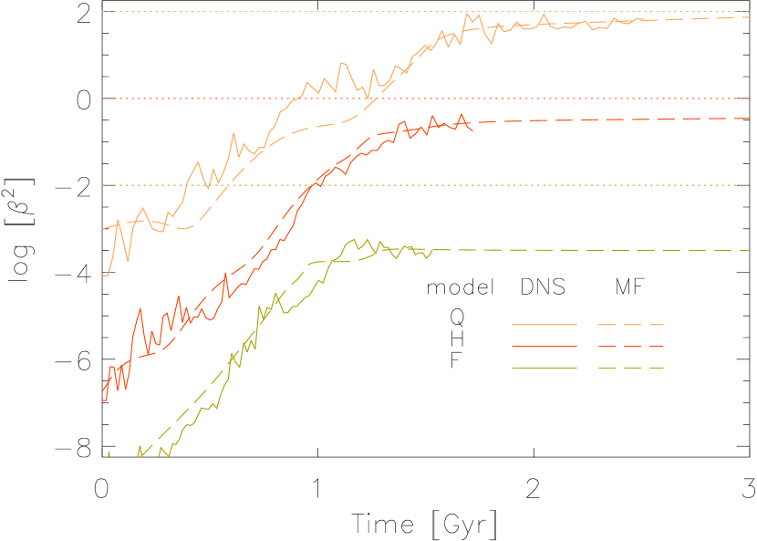
Figure 7: Evolution of the magnetic energy for the mean fields (normalised with the turbulent kinetic energy), i.e. $\beta^{2}$, from direct numerical simulations (DNS) and 1D dynamo simulations (MF). Different colours indicate the different supernova rates. The curves for model Q and F are shifted upwards and downwards, respectively, likewise the dotted horizontal lines at $log(E_{m}/E_{k})=2$, $0$ and $-2$ mark equipartition for models Q, H and F respectively. The growth and the saturation of the magnetic energy seen in the DNS is effectively reproduced via the 1D dynamo model using $\alpha$, $\eta$ and $\bar{u}_{z}$ with the quenching via Eqs. (16) and (17).

In the dynamical phase, due to the flattened profiles of $\alpha$ (and $\eta$) the amplification process slows down in the Q and H models, while it stops in model F. As illustrated in Fig. 7, where we compare the evolution of the magnetic energy in the direct simulations with the 1D dynamo model, the simple dynamo model does a reasonable job in reproducing the field evolution seen in DNS. Unlike in models Q and H, in model F, a non-vanishing contribution of the (${\bar{u}}_{z}+\gamma$) term is found to become important for comparatively smaller values of $\beta$ and the amplification of $\overline{\mathbf{B}}$ is inhibited as a result.

The sustained growth of the magnetic field appears to be a consequence of the combined quenching of $\alpha$ and $\eta$ – leading to an indefinitely growing field. This is also witnessed by the dynamo number $D$ (defined in Eq. (19) below), that becomes a function of $\beta$ according to Eq. (20). Only the growth time scale for the dynamo is reduced by the quenching of the diffusivity. This behaviour is clearly reflected in the 1D models for the cases Q and H, that show much reduced growth at late times. In contrast, in model F, at higher supernova rate, both the pumping, $\gamma$, and the wind, $\bar{u}_{z}$, appear to be less affected by the buildup of strong magnetic fields (see Fig. 5). In this situation it appears probable that the $\alpha\Omega$ dynamo is instead saturated by advective losses via the residual transport velocity ($\bar{u}_{z}+\gamma$). We have tested this scenario by switching off the transport term in all three models, which resulted in an endlessly growing field also for model F. We analytically justify this result in the following section. The effect of pumping and advective losses relative to the propagation direction of the dynamo wave has previously been studied in the kinematic phase only (see fig. 3 in Gressel et al., 2011).

The ability to reproduce the evolution of $\bar{B}_{x}(z)$ and $\bar{B}_{y}(z)$ profiles (as shown in the lower right panel in Fig. 2) using a simple one-dimensional $\alpha\Omega$ dynamo is rather remarkable. The space-time plots in this figure compares the evolution of the mean azimuthal field from 1D dynamo simulations (upper panel) and from DNS (lower panel) for model Q. The vertical scale heights and midplane field strengths of $\bar{B}_{x}(z)$ are also comparable for both of these simulations – see panels (a) and (b) in Fig. 2.

3.2.3 Assessment in terms of dynamo numbers

The time where the growth rate of $E_{\rm m}$ changes is clearly seen in Fig. 1. For instance, $E_{\rm m}$ saturates after $1.2$, $1$ and $0.9\,\rm Gyr$ for models Q, H and F, respectively. We were able to analytically derive the value of the total magnetic energy at the time where it changes its slope, and this is done as follows: The dynamo number for the $\alpha\Omega$ dynamo is defined as (e.g. Ruzmaikin et al., 1988),

$$D\equiv C_{\alpha}\times C_{\Omega}=\frac{\alpha H}{\eta}\times\frac{\Omega H^{2}}{\eta}=\frac{\alpha\ H^{3}\Omega}{\eta^{2}}\,,$$ (19)

where $C_{\alpha}$, and $C_{\Omega}$ denote the contributions from the $\alpha$ effect and the shear, respectively, and where $H$ is a typical vertical length scale. Substituting Eq. (16) into Eq. (19), we yield an expression for this number in terms of the supernova rate, $\sigma$, and the relative magnetic field strength, $\beta$, that is,

$$D=D_{0}\,\left(\frac{\sigma}{\sigma_{0}}\right)^{-0.4}\,\frac{\left(1+6\,\beta\right)^{2}}{1+27\,\beta^{2}}\,,$$ (20)

where $D_{0}$ is the unquenched dynamo number obtained with values for $\alpha$, and $\eta$ in the kinematic phase.

Assuming $\bar{u}_{z}(z)\simeq\gamma(z)$, and using the known approximate solution for the $\alpha\Omega$ dynamo for stationary profiles of the dynamo coefficients (similar to Shukurov, 1998), we obtain

$$\bar{B}(t)=\bar{B}_{0}\ \mathrm{exp}\left({\frac{t}{t_{\rm d}}\sqrt{\frac{D}{D_{\rm c}}-1}\,}\right)\,,$$ (21)

as an approximate solution expressed in terms of a diffusion time $t_{\rm d}\equiv H^{2}/\eta=\sigma^{-0.4}H^{2}\ (1+6\,\beta)/\eta_{0}$, derived from Eq. (16), and introducing the critical dynamo number, $D_{\rm c}$, delineating marginal growth of the dynamo. We choose $L=1\,\rm kpc$, and $\eta^{\prime}=1\,\rm kpc\,\rm km\,s^{-1}$ to normalise $H$ and $\eta_{0}$ as $H=H^{\prime}L$ and $\eta_{0}=\widetilde{\eta}\eta^{\prime}$. Using the appropriate relation (20) for the dynamo number, we further yield $\,\bar{B}(t)=\bar{B}_{0}\ \mathrm{exp}\left({f(\beta,\sigma)\,t}\right)\,$ with the function $f(\beta,\sigma)$ given by

$$f(\beta,\sigma)=\frac{\eta_{0}}{H^{2}}\ \sqrt{\frac{D_{0}}{D_{\rm c}}\frac{\sigma^{0.4}}{\left(1+27\beta^{2}\right)}-\frac{\sigma^{0.8}}{\left(1+6\beta\right)^{2}}}\,.$$ (22)

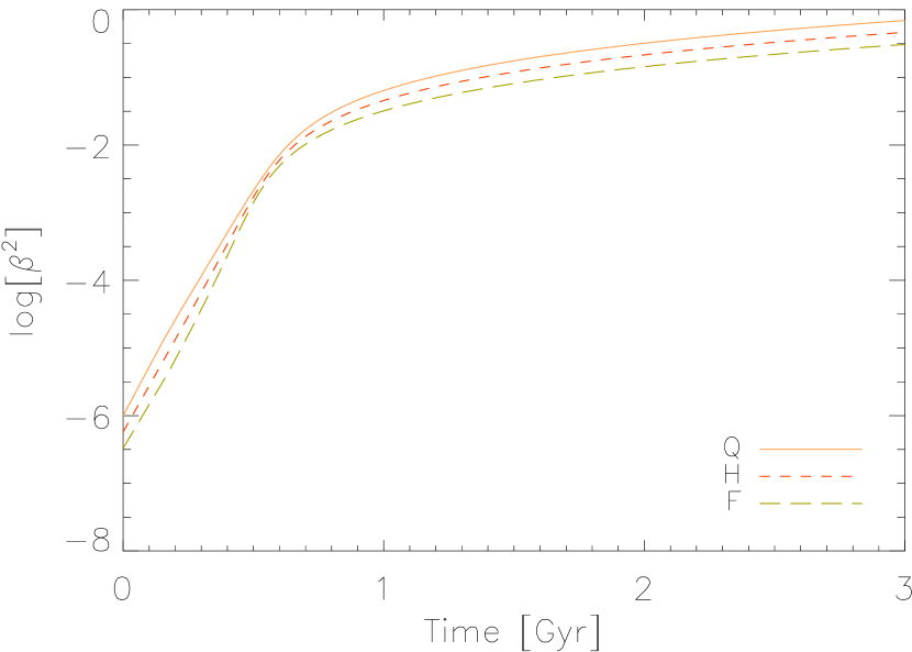
Figure 8: Evolution of the square of relative field strengths, $\beta^{2}$, for different SN rates calculated using Eqs. (21) and (22). The e-folding time of the initial kinematic phase (up to $\sim 1\,\rm Gyr$) is approximately $100\,\rm Myr$ (consistent with the DNS and the 1D-MF simulations).

This relation provides an evolution equation for the mean magnetic field. We plot the resulting time evolution of square of the relative magnetic field strength, $\beta^{2}$, in Fig. 8. Here, length scales are normalised with $H=1\,\rm kpc$, the ratio $D_{0}/D_{c}=3.5$ is obtained empirically from a set of 1D simulations, and $\eta_{0}=4.4\,\rm kpc\,\rm km\,s^{-1}$ is taken from Table 6. The values of $\bar{B}_{0}$ and the equipartition magnetic field are chosen according to the initial values of $\beta$ taken from the DNS, that is $\beta=6\times 10^{-4}\,\sigma^{-0.4}$. In particular, the factor $\sigma^{-0.4}$ derives from the square root of turbulent kinetic energy, $\rho^{0.5}\ u^{\prime}$, appearing in the denominator of Eq. (15). Unlike in the DNS, all three curves show a very similar behaviour. This is because the dynamical phase is not well reproduced in Eq. (22), since the quenching of the wind is not considered in our analytic description given by Eq. (21). Model Q (solid line), however, approximately mimics the entire evolution curve of $\beta$ seen in the DNS, suggesting that the effect of the outflow is less pronounced at low supernova rates.

To convert Eq. (21) into an evolution equation for the total magnetic energy, we use a relation between the average and turbulent fields as a function of $\sigma$ (also see Fig. 4):

$$|\overline{\mathbf{B}}|=0.27\sigma^{-0.30\pm 0.07}\,|\mathbf{b}^{\prime}|\,,$$ (23)

and express the total magnetic energy as a sum of the magnetic energy from the mean and turbulent fields. We finally obtain an evolution equation for the total magnetic energy,

$$E_{\rm m}=E_{0}\left(1+13.7\sigma^{0.6}\right)\,\mathrm{exp}\left(\;{2f(\beta,\sigma)\,t}\;\right)\,.$$ (24)

This evolution equation is valid for the initial kinematic phase of $E_{\rm m}$, that is, where Eq. (23) is valid. Substituting the values for $\sigma$ and $f(\beta,\sigma)$, for fixed $\beta$, in Eq. (24), we obtain a scaling for the total magnetic energy $E_{\rm m}$ at the end of the kinematic phase. This estimate successfully predicts the values obtained in DNS.

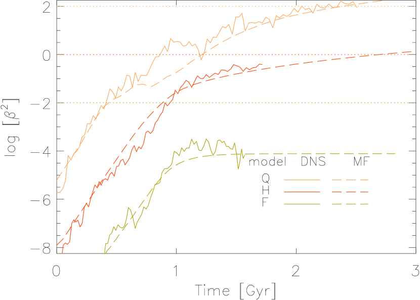
Figure 9: Same as Fig. 7, except the energies from DNS are computed within the inner disc ($|z|<0.5\,\rm kpc$), and the 1D mean-field simulations are preformed with the profiles of the dynamo coefficients restricted to the thin disc. The e-folding time for all models in the initial kinematic phase is $\sim 70\,\rm Myr$.

As is clear from Figs. 7 and 8, the $\beta$ values in any of our models do not exceed unity. This is partly because we have taken averages over the entire volume of the simulation domain. If we restrict ourselves to the thin disc ($|z|<0.5\,\rm kpc$), it is possible to obtain $\beta$ values exceeding unity, at least for smaller SN rates. This hypothesis is tested with 1D dynamo simulations using vertical profiles of $\alpha$, $\eta$, $\gamma$ and $\bar{u}_{z}$ that have been obtained within the range $-0.5\,\rm kpc<z<+0.5\,\rm kpc$. Using these, we obtain $\beta^{2}\sim 1.2$, $0.35$ and $0.03$ for model Q, H and F as shown in Fig. 9, where we plot magnetic energies computed from the thin disc. We also obtain faster growth times of $\sim 70\,\rm Myr$ for $\beta^{2}$ during the initial kinematic phase. The analytical solution given by Eq. (21), now using $H=0.25\,\rm kpc$ to account for the more localised dynamo mode, also yields $\beta^{2}\sim 1.5$ for all SN rates. In reality, $\beta$ should be smaller than unity for the models H and F – but since the quenching of the wind and pumping terms is not considered in the analytic approach, we obtain artificially high values from Eq. (21), again illustrating the importance of including proper vertical transport processes in the dynamo model.

4 Summary of results

The main results of the work that we have presented in the previous sections can be summarised as follows:

1. We observe a steady exponential amplification of the magnetic energy, $E_{\rm m}$, with a fast e-folding time $\sim 100\,\rm Myr$ during the entire kinematic growth phase.

2. In accordance with the derived dynamo numbers, the back-reaction of the mean magnetic field onto the turbulence does not saturate the dynamo, but instead only leads to an increase of the growth time. Dynamo saturation seems only possible via field removal by the wind.

3. Large-scale vertical structures (with ‘S’ mode parity) of the average magnetic field evolve within a $\,\rm Gyr$, with midplane field strengths of about $2-3\,\mu\rm G$, as seen in Fig. 2. Typical scale heights of the vertical exponential profile of the averaged magnetic field are about $850\,\rm pc$ in the central disc ($h_{0}$) and a few $\rm kpc$ within the upper halo ($h_{1}$) (see Table 5).

4. Scale heights of the inner disc $h_{0}$ are similar to the observations of nearby spiral galaxies by Krause (2011), values of $h_{1}$ however are almost half as compared to the observations under the assumption of equipartition between cosmic rays and magnetic field. The scale heights, $h_{i}$, are moreover found to scale roughly as $h_{0}\sim\sigma^{0.4}$ and $h_{1}\sim\sigma^{0.8}$, respectively.

5. We do not observe a noticeable contribution of the MRI in our simulations, that is, the final ${\overline{\mathbf{B}}}(z)$ profile and the ISM composition are similar for models with the same SN rate irrespective of the initial vertical flux. This is with the exception of the model ‘QS’, in which the initially strong ‘A’ mode persists in the dynamical phase, presumably due to the flux-preserving periodic boundary conditions.

6. During the kinematic phase, and once the mean field is sufficiently established (that is, around $\beta=10^{-2}$), the ratio of the mean-to-turbulent magnetic fields is found to scale with $\sigma^{-0.3}$ (see Fig. 4). This agrees with our previous results in the kinematic phase (Gressel et al., 2008a), and matches well the observations by Chyży (2008). This scaling relation does however not remain valid during the dynamical phase, which may be related to the correlation between midplane density and the SN rate. It has to be tested with a realistic density correlated variation of the SN-rate.

7. The average vertical density profiles to a first order scale exponentially with height, and can be approximated with typically three individual scale heights (listed in Table 2). The widths of the two thick components, $r_{1}$, and $r_{2}$, are found to scale roughly as $\sim\sigma^{0.4}$.

8. The average Alfvén velocities, $v_{\rm A}$, in the outer halo are approximately $30\,\rm km\,s^{-1}$, irrespective of $\sigma$. This is roughly equal to the turbulent velocities, $u^{\prime}$, for the cases with lower SN rates. We observe no statistical correlation between the Alfvén velocities and the mass density, $\rho$, which implies that it is possible to define the vertical profile of $v_{\rm A}$ as a ratio of averaged profiles of magnetic field and $\rho^{0.5}$.

9. The vertical structure of the ISM is maintained via a total pressure ($P_{\rm tot}$) equilibrium in all thermal components (except the hot ISM component), this composition remains unchanged during the dynamical phase (cf. Table 3).

10. Within the inner thin disc ($|z|<0.5\,\rm kpc$), the magnetic energy in the dynamical phase is not distributed uniformly in all ISM components (cf. Table 4). The comparatively largest ratio of $E_{\rm m}$ and $E_{\rm kin}$ is associated with the warm ionised medium and lowest with the hot component.

11. The comparatively largest fractions of magnetic to turbulent kinetic energy are reached in the models with smaller SN rates. If we consider the entire box ($|z|<2.1\,\rm kpc$), this ratio is still smaller than unity (i.e., $E_{\rm kin}>E_{\rm m}$), but within the inner disc ($|z|<0.5\,\rm kpc$) it exceeds 1 for model Q (see Table 4).

5 Conclusions

We have presented new results on the amplification of magnetic fields in the turbulent multi-phase interstellar medium. Extending our previous work, we have focused on the late evolution phase, where magnetic fields become dynamically important. Our main motivation has been to understand the different saturation behaviour at low and high supernova rates.

We have demonstrated that magnetic fields can be amplified up to equipartition with the turbulent kinetic energy in direct simulations of the turbulent ISM. However, in model F (with a set of parameters consistent with the Milky Way), the magnetic energy reached only one fifth of the kinetic energy. The reason may be an artificial mass loss by the wind in a still a too small box setup, but generally the behaviour seen in DNS can be accounted for by simplified mean-field models. The correlation of the mean azimuthal field with the pitch angle found in a sample of galaxies by Van Eck et al. (2015) is consistent with a partial saturation by the wind preserving the pitch angle.

As the key result of this paper, we were able to reproduce the evolution of $\bar{B}_{x}(z)$ and $\bar{B}_{y}(z)$ profiles into the saturated regime using a simple one-dimensional $\alpha\Omega$ dynamo model with algebraically quenched coefficients – notably including the mean vertical flow velocity $\bar{u}_{z}(z)$. We remark that this simplified approach should additionally be complemented with constraints arising from conservation of magnetic helicity (Sur et al., 2007), which may become more severe at higher magnetic Reynolds numbers (Del Sordo et al., 2013).

Furthermore, in a more realistic future scenario, one should include the coexistence of regions with strong and low star formation – as this would naturally be the case when looking at galaxies as a whole. Observable consequences of this situation can however only be studied in global models. Because the computational effort of a global simulation with the resolution similar to the local models still exceeds current high performance compute facilities, the use of dynamical mean-field models is the way to further analyse these questions. The striking agreement seen in the lower right panel of Fig. 2, however, strongly advertises the mean-field approach as a powerful tool in understanding the evolution of the large-scale ordered fields in the diffuse interstellar medium – even into the realm of dynamically important magnetic fields.

A further unknown aspect is the influence of cosmic rays on the amplification and saturation of the dynamo. The turbulence may destroy the anisotropic cosmic ray diffusion and therefore inhibit dynamo action by cosmic rays. On the other hand, the cosmic ray pressure may influence the turbulent transport processes and eventually change the dynamo properties.