D-vine copula based quantile regression

Abstract

Quantile regression, that is the prediction of conditional quantiles, has steadily gained importance in statistical modeling and financial applications. The authors introduce a new semiparametric quantile regression method based on sequentially fitting a likelihood optimal D-vine copula to given data resulting in highly flexible models with easily extractable conditional quantiles. As a subclass of regular vine copulas, D-vines enable the modeling of multivariate copulas in terms of bivariate building blocks, a so-called pair-copula construction (PCC). The proposed algorithm works fast and accurate even in high dimensions and incorporates an automatic variable selection by maximizing the conditional log-likelihood. Further, typical issues of quantile regression such as quantile crossing or transformations, interactions and collinearity of variables are automatically taken care of. In a simulation study the improved accuracy and saved computational time of the approach in comparison with established quantile regression methods is highlighted. An extensive financial application to international credit default swap (CDS) data including stress testing and Value-at-Risk (VaR) prediction demonstrates the usefulness of the proposed method.

Keywords: quantile regression, conditional distribution, vine copula, conditional copula quantile, stress testing

1 Introduction

Predicting quantiles (e.g. median or quartiles) of a random variable conditioned on other variables taking on fixed values, has continually attracted interest and found applications in various fields, especially in finance. It has become a standard tool for risk managers working on portfolio optimization, asset pricing and the evaluation of systemic risk. For example, Adrian and Brunnermeier (2016) introduce the CoVaR, a measure for systemic risk calculating conditional quantiles of a financial institution’s loss distribution conditional on other institutions being in distress, and use it to evaluate the institution’s contribution to systemic risk. A similar approach to measure systemic risk is found in Brownlees and Engle (2012). Further applications of quantile regression in the financial sector include measuring dependence in the FX markets (Bouyé and Salmon, 2009), developing pricing models for real estates (Li et al., 2013) and predicting volatilities in the stock market (Noh et al., 2015).
The literature is quite rich in methods to predict conditional quantiles. The most famous and therefore frequently used method is linear quantile regression (Koenker and Bassett, 1978) which can be seen as the expansion of the well known ordinary least squares estimation used to predict conditional means. These simple linear models have been refined to account for nonparametric effects via additive models (Koenker, 2011; Fenske et al., 2012). Further methods include local quantile regression (Spokoiny et al., 2013), single-index quantile regression (Wu et al., 2010), semiparametric quantile regression (Noh et al., 2015), nonparametric quantile regression (Li et al., 2013) and quantile regression for time series (e.g. Chen et al., 2009; Xiao and Koenker, 2009). In the machine learning context, Hwang and Shim (2005) use support vector machines for conditional quantile estimation while random forests are utilized in Meinshausen (2006). Moreover, Bouyé and Salmon (2009) propose a general approach to nonlinear quantile regression with one predictor based on a copula function.

The linear quantile regression method by Koenker and Bassett (1978) has been criticized by Bernard and Czado (2015) for imposing too restrictive assumptions on the shape of the regression quantiles. They show that for normally distributed marginals the model is misspecified as soon as the underlying dependence structure between response and covariates deviates from a Gaussian copula. Further, the method suffers from issues like quantile crossing and from the typical pitfalls of linear models such as multicollinearity, selection and significance of covariates and the inclusion of interactions or transformed variables.

In contrast, the methodology proposed in this paper makes no precise assumptions about the shape of the conditional quantiles. The dependence relationship between response and covariates is modeled flexibly using a parametric D-vine copula, a subclass of regular vine copulas which have enhanced statistical modeling since the publication of the seminal paper of Aas et al. (2009). Then, as we will show, the model’s conditional quantiles can be extracted analytically without approximations or excessive computational effort. As is usual when working with copulas, we further gain from the added flexibility of separating marginal and dependence modeling.

One of the main contributions of this work is a new algorithm that sequentially fits such a regression D-vine copula to given copula data, exhibiting many desirable features. On the one hand, step by step, the algorithm adds covariates to the regression model with the objective of maximizing a conditional likelihood, i.e. the likelihood of the predictive model of the response given the covariates. On the other hand, an automatic variable selection is incorporated, meaning that the algorithm will stop adding covariates to the model as soon as none of the remaining covariates is able to significantly increase the model’s conditional likelihood. This results in parsimonious and at the same time flexible models whose conditional quantiles may strongly deviate from linearity. Due to the model construction, quantile crossings do not occur. Thus, the resulting D-vine quantile regression is able to overcome all the shortcomings of classical linear quantile regression mentioned above and therefore adds a new (and as we will see competitive) approach to the existing research on quantile regression.

The remainder of the paper is organized as follows. Section 2 introduces the concept of D-vines while Section 3 describes how they can be used for the prediction of conditional quantiles. Further, we demonstrate the usefulness of the approach in a simulation study. The prediction performance of D-vine quantile regression and its competitor methods, which are discussed in Section 4, is presented in Section 5. For the demonstration of the usefulness of our method we include a real data example in Section 6 that contains financial applications of the D-vine quantile regression featuring stress testing and Value-at-Risk prediction. Section 7 gives conclusions and areas of future research.

2 D-vine copulas

A $d$-dimensional copula $C$ is a $d$-variate distribution function on the unit hypercube $[0,1]^{d}$ with uniform marginal distribution functions. Sklar’s Theorem (Sklar, 1959) provides a link between multivariate distributions and their associated copulas. It states that for every multivariate random vector $\mathbf{X}=(X_{1},\ldots,X_{d})^{\prime}\sim F$ with marginal distribution functions $F_{1},\ldots,F_{d}$, there exists a copula $C$ associated with $\mathbf{X}$, such that $F(x_{1},\ldots,x_{d})=C(F_{1}(x_{1}),\ldots,F_{d}(x_{d}))$. This decomposition of the multivariate distribution into its margins and its associated copula is unique when $\mathbf{X}$ is absolutely continuous (which we will assume for the remainder of this paper). In that case, the density of $\mathbf{X}$ can be decomposed similarly: $f(x_{1},\ldots,x_{d})=c(F_{1}(x_{1}),\ldots,F_{d}(x_{d}))f_{1}(x_{1})\cdot\ldots\cdot f_{d}(x_{d})$, where $c(u_{1},\ldots,u_{d}):=\frac{\partial^{d}}{\partial_{1}\cdots\partial_{d}}C(u_{1},\ldots,u_{d})$ is the copula density and $f_{1},\ldots,f_{d}$ are the marginal densities.
If we are interested solely in the dependence structure of $\mathbf{X}$, we considered it on the so-called u-scale (or copula scale) by applying the probability integral transform (PIT) to its marginals: $U_{j}:=F_{j}(X_{j})$, $j=1,\ldots,d$. The $U_{j}$ are then uniformly distributed and their joint distribution function is the copula $C$ associated with $\mathbf{X}$. Refer to Joe (1997) and Nelsen (2007) for a detailed examination of copulas including many examples of parametric copulas, especially bivariate pair-copulas. Those are of special interest to us since they are the building blocks used for the pair-copula construction of D-vines.

For a random vector $\mathbf{X}$, a set $D\subset\left\{1,\ldots,d\right\}$ and $i,j\in\left\{1,\ldots,d\right\}\backslash D$ we use the following notations:

1. $C_{X_{i},X_{j};\mathbf{X}_{D}}(\cdot,\cdot;\mathbf{x}_{D})$ denotes the copula associated with the conditional distribution of $(X_{i},X_{j})^{\prime}$ given $\mathbf{X}_{D}=\mathbf{x}_{D}$. We abbreviate this by $C_{ij;D}(\cdot,\cdot;\mathbf{x}_{D})$. Further, $c_{ij;D}(\cdot,\cdot;\mathbf{x}_{D})$ is the copula density corresponding to $C_{ij;D}(\cdot,\cdot;\mathbf{x}_{D})$.

2. $F_{X_{i}|\mathbf{X}_{D}}(\cdot,\cdot|\mathbf{x}_{D})$ denotes the conditional distribution of the random variable $X_{i}$ given $\mathbf{X}_{D}=\mathbf{x}_{D}$. We use $F_{i|D}(\cdot,\cdot|\mathbf{x}_{D})$ as an abbreviation.

3. $C_{U_{i}|\mathbf{U}_{D}}(\cdot,\cdot|\mathbf{u}_{D})$ denotes the conditional distribution of the PIT random variable $U_{i}$ given $\mathbf{U}_{D}=\mathbf{u}_{D}$. We abbreviate this by $C_{i|D}(\cdot,\cdot|\mathbf{u}_{D})$.

Following Czado (2010), the joint density $f$ of the continuously distributed random vector $\mathbf{X}$ can be written in terms of (conditional) bivariate copula densities and its marginal densities as

$$f(x_{1},\ldots,x_{d})=\prod_{k=1}^{d}{f_{k}(x_{k})}\prod_{i=1}^{d-1}\prod_{j=i+1}^{d}c_{ij;i+1,\ldots,j-1}\big{(}F_{i|i+1,\ldots,j-1}\left(x_{i}|x_{i+1},\ldots,x_{j-1}\right),\\ F_{j|i+1,\ldots,j-1}\left(x_{j}|x_{i+1},\ldots,x_{j-1}\right);x_{i+1},\ldots,x_{j-1}\big{)}.$$ (2.1)

We call this pair-copula construction (PCC) a D-vine density with order $X_{1}$–$X_{2}$–$\ldots$–$X_{d}$. If all margins are uniform, we speak of a D-vine copula. As introduced by Bedford and Cooke (2002) we present a graph theoretic representation of the D-vine, where each edge of the graph corresponds to a pair-copula.

Example .

Figure 1 shows an exemplary 5-dimensional D-vine corresponding with

$$f(x_{1},x_{2},x_{3},x_{4},x_{5})= f_{1}(x_{1})f_{2}(x_{2})f_{3}(x_{3})f_{4}(x_{4})f_{5}(x_{5})$$

$$\cdot c_{12}\cdot c_{23}\cdot c_{34}\cdot c_{45} T_{1}$$ ()

$$\cdot c_{13;2}\cdot c_{24;3}\cdot c_{35;4} T_{2}$$ ()

$$\cdot c_{14;23}\cdot c_{25;34} T_{3}$$ ()

$$\cdot c_{15;234}, T_{4}$$ ()

where for brevity we omitted the arguments of the pair-copulas.

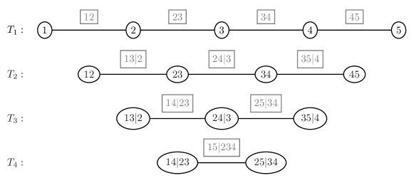
Figure 1: Graph theoretic representation of a D-vine with order $X_{1}$–$X_{2}$–$X_{3}$–$X_{4}$–$X_{5}$. The nodes of the trees are plotted in black circles and the corresponding pair-copulas in gray squares.

We see that all pair-copulas used in the decomposition appear as edges in the corresponding nested set of trees displayed in Figure 1.

In order to fit a D-vine copula with a fixed order to given data, all pair-copulas appearing in Equation (missing) 2.1 are estimated as parametric bivariate copulas. A common assumption when working with D-vines is to assume that the copulas associated with conditional distributions $c_{i,j;D}$ do not depend on the specific values of the conditioning vector $\mathbf{x}_{D}$, i.e. $c_{i,j;D}(\cdot,\cdot;\mathbf{x}_{D})\equiv c_{i,j;D}(\cdot,\cdot)$. A more detailed examination of this so-called simplifying assumption can for example be found in Stöber et al. (2013), Hobæk Haff et al. (2010), Killiches et al. (2016a) and Killiches et al. (2016c).
The conditional distributions $F_{i|D}\left(x_{i}|\mathbf{x}_{D}\right)$ appearing in the PCC can be evaluated using only the pair-copulas specified for the D-vine from lower trees by applying the following recursion, which was first stated by Joe (1997): Let $l\in D$ and $D_{-l}:=D\backslash\left\{l\right\}$. Then,

$$F_{i|D}\left(x_{i}|\mathbf{x}_{D}\right)=h_{i|l;D_{-l}}\left(F_{i|D_{-l}}\left(x_{i}|\mathbf{x}_{D_{-l}}\right)|F_{l|D_{-l}}\left(x_{l}|\mathbf{x}_{D_{-l}}\right)\right),$$ (2.2)

where for $i,j\notin D,i<j$, $h_{i|j;D}(u|v)={\partial C_{ij;D}(u,v)}/{\partial v}=C_{i|j;D}(u|v)$ and analogously $h_{j|i;D}(u|v)={\partial C_{ij;D}(u,v)}/{\partial u}=C_{j|i;D}(u|v)$ are the h-functions associated with the pair-copula $C_{ij;D}$.
In Section 2 the first argument of $c_{14;23}$ from Tree 3, namely $F_{1|23}(x_{1}|x_{2},x_{3})$, can be evaluated using the h-functions associated with $C_{13;2}$, $C_{12}$ and $C_{23}$ from the first two trees:

$$F_{1|23}(x_{1}|x_{2},x_{3})=h_{1|3;2}(F_{1|2}(x_{1}|x_{2})|F_{3|2}(x_{3}|x_{2}))=h_{1|3;2}(h_{1|2}(F_{1}(x_{1})|F_{2}(x_{2}))|h_{3|2}(F_{3}(x_{3})|F_{2}(x_{2}))).$$

3 D-vine based quantile regression model

3.1 Conditional quantile function

The main purpose of D-vine copula based quantile regression is to predict the quantile of a response variable $Y$ given the outcome of some predictor variables $X_{1},\ldots,X_{d}$, $d\geq 1$, where $Y\sim F_{Y}$ and $X_{j}\sim F_{j}$, $j=1,\ldots,d$. Hence, the focus of interest lies on the joint modeling of $Y$ and $\mathbf{X}$ and in particular on the conditional quantile function for $\alpha\in\left(0,1\right)$:

$$q_{\alpha}(x_{1},\ldots,x_{d}):=F^{-1}_{Y|X_{1},\ldots,X_{d}}(\alpha|x_{1},\ldots,x_{d}).$$ (3.3)

Using the probability integral transforms $V:=F_{Y}(Y)$ and $U_{j}:=F_{j}(X_{j})$ with corresponding PIT values $v:=F_{Y}(y)$ and $u_{j}:=F_{j}(x_{j})$, it follows that

$$F_{Y|X_{1},\ldots,X_{d}}(y|x_{1},\ldots,x_{d}) =P(Y\leq y|X_{1}=x_{1},\ldots,X_{d}=x_{d})$$

$$=P(F_{Y}(Y)\leq v|F_{1}(X_{1})=u_{1},\ldots,F_{d}(X_{d})=u_{d})$$

$$=C_{V|U_{1},\ldots,U_{d}}(v|u_{1},\ldots,u_{d}).$$

Therefore, inversion yields

$$F^{-1}_{Y|X_{1},\ldots,X_{d}}(\alpha|x_{1},\ldots,x_{d})=F^{-1}_{Y}\left(C^{-1}_{V|U_{1},\ldots,U_{d}}(\alpha|u_{1},\ldots,u_{d})\right).$$ (3.4)

Hence, the conditional quantile function can be expressed in terms of the inverse marginal distribution function $F^{-1}_{Y}$ of the response $Y$ and the conditional copula quantile function $C^{-1}_{V|U_{1},\ldots,U_{d}}$ conditioned on the PIT values of $\mathbf{x}$. Note that this result was already stated for the one-dimensional predictor case in Equation (2) of Bernard and Czado (2015).
Now, we can obtain an estimate of the conditional quantile function by estimating the marginals $F_{Y}$ and $F_{j}$, $j=1,\ldots,d$, as well as the copula $C_{V,U_{1},\ldots,U_{d}}$ and plugging them into Equation (missing) 3.4:

$$\hat{q}_{\alpha}(x_{1},\ldots,x_{d}):=\hat{F}^{-1}_{Y}\left(\hat{C}^{-1}_{V|U_{1},\ldots,U_{d}}(\alpha|\hat{u}_{1},\ldots,\hat{u}_{d})\right),$$ (3.5)

where $\hat{u}_{j}:=\hat{F}_{j}(x_{j})$ is the estimated PIT of $x_{j}$, $j=1,\ldots,d$.
While regarding the $\hat{F}_{j}$ there is a vast literature about the estimation of a univariate CDF, the question arises how to estimate the multivariate copula $C_{V,U_{1},\ldots,U_{d}}$, such that on the one hand it facilitates a flexible model that is able to capture asymmetric dependencies, heavy tails and tail dependencies between the variables, and on the other hand the estimated conditional quantile function $\hat{C}^{-1}_{V|U_{1},\ldots,U_{d}}(\alpha|\hat{u}_{1},\ldots,\hat{u}_{d})$ is easily calculable. The answer we suggest is to fit a D-vine copula to $(V,U_{1},\ldots,U_{d})^{\prime}$, such that $V$ is the first node in the first tree (i.e. a D-vine with order $V$–$U_{l_{1}}$–$\ldots$–$U_{l_{d}}$, where $(l_{1},\ldots,l_{d})^{\prime}$ is allowed to be an arbitrary permutation of $(1,\ldots,d)^{\prime}$). This results in a flexible class of copulas since each bivariate copula of the pair-copula construction can be modeled separately and the order of the $U_{j}$ is a parameter that can be chosen such that the conditional likelihood is maximized as will be explained in detail in the next section. Finally, the recursion given in Equation (missing) 2.2 allows us to express $C_{V|U_{1},\ldots,U_{d}}(v|u_{1},\ldots,u_{d})$ in terms of nested h-functions and consequently, $C^{-1}_{V|U_{1},\ldots,U_{d}}(\alpha|u_{1},\ldots,u_{d})$ in terms of inverse h-functions. We will now demonstrate this in a 4-dimensional example.

Example .

For a D-vine with order $V$–$U_{1}$–$U_{2}$–$U_{3}$, using Equation (missing) 2.2 the conditional distribution of $V$ given $(U_{1},U_{2},U_{3})^{\prime}$ can recursively be expressed as

$$C_{V|U_{1},U_{2},U_{3}}(v|u_{1},u_{2},u_{3}) =h_{V|U_{3};U_{1},U_{2}}(C_{V|U_{1},U_{2}}(v|u_{1},u_{2})|C_{U_{3}|U_{1},U_{2}}(u_{3}|u_{1},u_{2}))$$

$$=h_{V|U_{3};U_{1},U_{2}}(h_{V|U_{2};U_{1}}(C_{V|U_{1}}(v|u_{1})|C_{U_{2}|U_{1}}(u_{2}|u_{1}))|$$

$$\qquad\qquad\qquad h_{U_{3}|U_{1};U_{2}}(C_{U_{3}|U_{2}}(u_{3}|u_{2})|C_{U_{1}|U_{2}}(u_{1}|u_{2})))$$

$$=h_{V|U_{3};U_{1},U_{2}}(h_{V|U_{2};U_{1}}(h_{V|U_{1}}(v|u_{1})|h_{U_{2}|U_{1}}(u_{2}|u_{1}))|$$

$$\qquad\qquad\qquad h_{U_{3}|U_{1};U_{2}}(h_{U_{3}|U_{2}}(u_{3}|u_{2})|h_{U_{1}|U_{2}}(u_{1}|u_{2}))).$$

Inversion yields the conditional quantile function:

$$\begin{split}&C^{-1}_{V|U_{1},U_{2},U_{3}}(\alpha|u_{1},u_{2},u_{3})=\\ &h^{-1}_{V|U_{1}}\left[h^{-1}_{V|U_{2};U_{1}}\left\{h^{-1}_{V|U_{3};U_{1},U_{2}}\Big{(}\alpha\big{|}h_{U_{3}|U_{1};U_{2}}\big{(}h_{U_{3}|U_{2}}(u_{3}|u_{2})\big{|}h_{U_{1}|U_{2}}(u_{1}|u_{2})\big{)}\Big{)}\Big{|}h_{U_{2}|U_{1}}(u_{2}|u_{1})\right\}\Big{|}u_{1}\right].\end{split}$$

Note that $C^{-1}_{V|U_{1},\ldots,U_{d}}(\alpha|u_{1},\ldots,u_{d})$ is monotonically increasing in $\alpha$. Therefore, a crossing of quantile functions corresponding to different quantile levels is not possible. This issue of quantile crossing often arises in linear and non-linear quantile regression (e.g. see the application section of Fenske et al., 2012). Bernard and Czado (2015) show that in linear regression quantile functions may cross if non-Gaussian data is modeled. In addition, in (non-)linear quantile regression a substantial amount of effort has to be put into dealing with issues such as transforming response and covariates, including interactions among covariates and avoiding collinearity between covariates. Our approach solves these issues automatically since the distribution class given by the D-vines is much more flexible and makes less restrictive model assumptions how the covariates influence the response. This is also noted for regular vine regression by Cooke et al. (2015).

3.2 Estimation process

This section explains how the estimate of $q_{\alpha}(\mathbf{x})$ is obtained using a two step estimation procedure. All numerical calculations are done using the programming language R (R Core Team, 2016) using the package VineCopula (Schepsmeier et al., 2016).
Let $\mathbf{y}:=\left(y^{(i)}\right)_{i=1,\ldots,n}$, $\mathcal{X}:=\big{(}x^{(i)}_{j}\big{)}_{j=1,\ldots,d,\ i=1,\ldots,n}$ be $n$ independent and identically distributed observations of the random vector $\left(Y,X_{1},X_{2},\ldots,X_{d}\right)^{\prime}$. The representation of $\hat{q}_{\alpha}(\mathbf{x})$ in Equation (missing) 3.5 allows us to divide the estimation process into two steps. In the first step we estimate the marginal distribution functions $F_{Y}$ and $F_{j}$ of $Y$ and $X_{j}$, $j=1,\ldots,d$, respectively, and in the second step the D-vine that specifies the pair copulas needed to evaluate $\hat{C}^{-1}_{V|U_{1},\ldots,U_{d}}(\alpha|\hat{u}_{1},\ldots,\hat{u}_{d})$ is estimated.

First step: estimation of the marginals

In general, we have two choices of how to fit the marginal distributions, either parametrically or nonparametrically. Since we will fit the copula in the second step parametrically, this choice will either result in a fully parametric or semiparametric estimate of $q_{\alpha}(\mathbf{x})$. Noh et al. (2013) point out that modeling the marginals as well as the copula parametrically might cause the resulting fully parametric estimator to be biased and inconsistent if one of the parametric models is misspecified. Therefore we prefer the semiparametric approach and estimate the marginals nonparametrically. Since we later need the inverse of the estimated marginals for the quantile prediction (c.f. Equation (missing) 3.5) we do not want to use the discrete valued ECDF for the estimation. Thus we choose the continuous kernel smoothing estimator (Parzen, 1962), which is, given a sample $\left(x^{(i)}\right)_{i=1,\ldots,n}$, defined as

$$\hat{F}(x)=\frac{1}{n}\sum_{i=1}^{n}{K\left(\frac{x-x^{(i)}}{h}\right)},\ x\in\mathbb{R},$$ (3.6)

where $K(x):=\int_{-\infty}^{x}k(t)dt$ with $k(\cdot)$ being a symmetric probability density function and $h>0$ a bandwidth parameter. Usually, we choose $k=\varphi$, i.e. a Gaussian kernel, and the plug-in bandwidth developed in Duong (2016), Equation (4), which minimizes the asymptotic mean integrated squared error (implemented in the function kcde of the package ks (Duong, 2015)).
Hence, we obtain $\hat{F}_{Y}$ and $\hat{F}_{j}$ as estimates for the marginal distribution functions. We use these to transform the observed data to pseudo copula data $\hat{v}^{(i)}:=\hat{F}_{Y}\left(y^{(i)}\right)$ and $\hat{u}^{(i)}_{j}:=\hat{F}_{j}\big{(}x^{(i)}_{j}\big{)}$, $j=1,\ldots,d$, $i=1,\ldots,n$. The pseudo copula data $\hat{\mathbf{v}}=\left(\hat{v}^{(i)}\right)_{i=1,\ldots,n}$, $\hat{\mathcal{U}}=\big{(}\hat{u}^{(i)}_{j}\big{)}_{j=1,\ldots,d,\ i=1,\ldots,n}$ is then an approximately i.i.d. sample from the PIT random vector $(V,U_{1},\ldots,U_{d})^{\prime}$ and will be used to estimate the D-vine copula in the second step.

Second step: estimation of the D-vine

As motivated by Equation (missing) 3.5, we fit a D-vine with order $V$–$U_{l_{1}}$–$\ldots$–$U_{l_{d}}$ to the pseudo copula data, since then the evaluation of $\hat{C}^{-1}_{V|U_{1},\ldots,U_{d}}(\alpha|\hat{u}_{1},\ldots,\hat{u}_{d})$ which is needed to calculate the conditional quantile is easily feasible. For this to work the ordering $\bm{l}=(l_{1},\ldots,l_{d})^{\prime}$ can generally be chosen arbitrarily. However, since the explanatory power of the resulting model does depend on the particular ordering, we want to choose it such that the resulting model for the prediction of the conditional quantile has the highest explanatory power. Since it would be infeasible to compare all $d!$ possible orderings, we propose a new algorithm that automatically constructs the D-vine sequentially choosing the most influential covariates. Similar to the step function for sequential estimation of linear models (cf. Venables and Ripley, 2002), starting with zero covariates, in each step we add the covariate to the model that improves the model’s fit the most. As a measure for the model’s fit, we define the conditional log-likelihood ($\operatorname{cll}$) of an estimated D-vine copula with ordering $\bm{l}$, estimated parametric pair-copula families $\hat{\bm{\mathcal{F}}}$ and corresponding copula parameters $\hat{\bm{\theta}}$ given pseudo copula data $(\hat{\mathbf{v}},\hat{\mathcal{U}})$ as

$$\operatorname{cll}\left(\bm{l},\hat{\bm{\mathcal{F}}},\hat{\bm{\theta}};\hat{\mathbf{v}},\hat{\mathcal{U}}\right):=\sum_{i=1}^{n}{\ln c_{V|\mathbf{U}}\left(\hat{v}^{(i)}|\hat{\mathbf{u}}^{(i)};\bm{l},\hat{\bm{\mathcal{F}}},\hat{\bm{\theta}}\right)}.$$ (3.7)

The conditional copula density $c_{V|\mathbf{U}}$ can be expressed as the product over all pair-copulas of the D-vine that contain $V$ (see Killiches et al., 2016b):

$$c_{V|\mathbf{U}}\left(\hat{v}^{(i)}|\hat{\mathbf{u}}^{(i)};\bm{l},\hat{\bm{\mathcal{F}}},\hat{\bm{\theta}}\right)=c_{VU_{l_{1}}}(\hat{v}^{(i)},\hat{u}_{l_{1}}^{(i)};\hat{\mathcal{F}}_{VU_{l_{1}}},\hat{\theta}_{VU_{l_{1}}})\times\\ \prod_{j=2}^{d}c_{VU_{l_{j}};U_{l_{1}},\ldots,U_{l_{j-1}}}\Big{(}\hat{C}_{V|U_{l_{1}},\ldots,U_{l_{j-1}}}\big{(}\hat{v}^{(i)}|\hat{u}_{l_{1}}^{(i)},\ldots,\hat{u}_{l_{j-1}}^{(i)}\big{)},\hat{C}_{U_{l_{j}}|U_{l_{1}},\ldots,U_{l_{j-1}}}\big{(}\hat{u}_{l_{j}}^{(i)}|\hat{u}_{l_{1}}^{(i)},\ldots,\hat{u}_{l_{j-1}}^{(i)}\big{)};\\ \hat{\mathcal{F}}_{VU_{l_{j}};U_{l_{1}},\ldots,U_{l_{j-1}}},\hat{\theta}_{VU_{l_{j}};U_{l_{1}},\ldots,U_{l_{j-1}}}\Big{)},$$

where $\hat{\mathcal{F}}_{I}$ and $\hat{\theta}_{I}$ denote the estimated family and parameter(s) of pair-copula $c_{I}$.
We now describe the D-vine regression algorithm which sequentially constructs a D-vine while maximizing the model’s conditional log-likelihood in each step (for a detailed code see Appendix A). Assume that at the beginning of the $k$th step of the algorithm the current optimal D-vine contains $k-1$ predictors (for illustration, see the black D-vine in Figure 2). For each of the remaining variables $U_{j}$ that have not been chosen yet, we fit the pair-copulas that are needed to extend the current model to a D-vine with order $V$–$U_{l_{1}}$–$\ldots$–$U_{l_{k-1}}$–$U_{j}$ (see the gray circles) and compute the resulting model’s conditional log-likelihood. Then, the current model is updated by adding the variable corresponding to the highest $\operatorname{cll}$, concluding step $k$. That way, step by step the covariates are ordered regarding their power to predict the response.

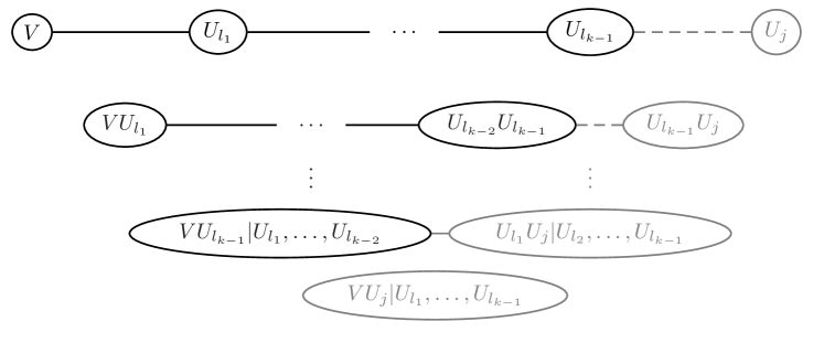
Figure 2: Extending the current D-vine (black) by adding $U_{j}$ in the $k$-th step of the algorithm. For this purpose, the gray pair-copulas have to be estimated.

In the case that in the $k$th step none of the remaining covariates is able to increase the model’s $\operatorname{cll}$, the algorithm stops and returns the model only containing the $k-1$ chosen covariates so far. Therefore, an automatic forward covariate selection is accomplished resulting in parsimonious models. In order to get even more parsimonious models, we also consider two variants of the $\operatorname{cll}$ penalizing the number of parameters $|\hat{\bm{\theta}}|$ used for the construction of the D-vine: the AIC-corrected conditional log-likelihood $\operatorname{cll}^{\operatorname{AIC}}$, defined as

$$\operatorname{cll}^{\operatorname{AIC}}\left(\bm{l},\hat{\bm{\mathcal{F}}},\hat{\bm{\theta}};\hat{\mathbf{v}},\hat{\mathcal{U}}\right):=-2\operatorname{cll}\left(\bm{l},\hat{\bm{\mathcal{F}}},\hat{\bm{\theta}};\hat{\mathbf{v}},\hat{\mathcal{U}}\right)+2|\hat{\bm{\theta}}|$$

and the BIC-corrected conditional log-likelihood $\operatorname{cll}^{\operatorname{BIC}}$, defined as

$$\operatorname{cll}^{\operatorname{BIC}}\left(\bm{l},\hat{\bm{\mathcal{F}}},\hat{\bm{\theta}};\hat{\mathbf{v}},\hat{\mathcal{U}}\right):=-2\operatorname{cll}\left(\bm{l},\hat{\bm{\mathcal{F}}},\hat{\bm{\theta}};\hat{\mathbf{v}},\hat{\mathcal{U}}\right)+\log(n)|\hat{\bm{\theta}}|.$$

Depending on how parsimonious the resulting model is desired to be, one can decide which version of the conditional log-likelihood to use. In our applications in the later sections we always use the AIC-corrected $\operatorname{cll}^{\operatorname{AIC}}$ since in the simulation study it has shown to select the most reasonable models in the sense that unimportant variables are disregarded and influential ones are kept in most of the instances.

Example .

We illustrate how the algorithm works for a four-dimensional data set $(y^{(i)},x^{(i)}_{1},x^{(i)}_{2},x^{(i)}_{3})^{\prime}$, $i=1,\ldots,n=500$, sampled from $(Y,X_{1},X_{2},X_{3})^{\prime}\sim\mathcal{N}_{4}(\mathbf{0},\Sigma)$ with

$$\Sigma=\begin{pmatrix}1&0.4&0.8&0\\ 0.4&1&0.32&0\\ 0.8&0.32&1&0\\ 0&0&0&1\\ \end{pmatrix}.$$

First, the data is transformed to pseudo copula data $(\hat{v}^{(i)},\hat{u}^{(i)}_{1},\hat{u}^{(i)}_{2},\hat{u}^{(i)}_{3})^{\prime}$, $i=1,\ldots,n$, using the kernel smoothing estimators introduced in Equation (missing) 3.6.

In the first step of the algorithm, for each of the pairs $(V,U_{j})^{\prime}$, $j=1,2,3$, the AIC-optimal pair-copula is chosen using the function BiCopSelect of the R package VineCopula with an independence test at level 0.05 (as described in Genest and Favre, 2007). Further, the conditional log-likelihood is calculated for each of the pairs (we omit the AIC- and BIC-corrected $\operatorname{cll}$-values here, since the fitted models have the same number of parameters and therefore these statistics would imply the same conclusions). The results are shown in the Table 1. Implying the largest $\operatorname{cll}$, $U_{2}$ is chosen as the first variable to construct the D-vine.

Pair-copula	$\hat{C}_{V,U_{1}}$	$\hat{C}_{V,U_{2}}$	$\hat{C}_{V,U_{3}}$
Family	Gauss	Gauss	Indep
Parameter	$0.34$	$0.79$	$0$
$\operatorname{cll}$	$33.0$	$249.4$	$0$

Table 1: Candidate models with corresponding $\operatorname{cll}$ after the algorithm’s first step.

In the second step, we investigate whether the addition of either of the remaining variables $U_{1}$ or $U_{3}$ to the current D-vine can improve the conditional log-likelihood of the model. Adding $U_{1}$ would update the D-vine to order $V$–$U_{2}$–$U_{1}$ with newly estimated pair-copulas $\hat{C}_{V,U_{1};U_{2}}$ (Gaussian with $\rho=0.27$) and $\hat{C}_{U_{1},U_{2}}$ (Gaussian with $\rho=0.23$). The log-likelihood of the resulting conditional copula $\hat{c}_{V|U_{2},U_{1}}$ is $269.8$. The addition of $U_{3}$ would result in both new pair-copulas to be estimated as independence copulas. Consequently, the conditional log-likelihood would not improve compared to the model without $U_{3}$. Since $269.8>249.4$, we update the vine to order $V$–$U_{2}$–$U_{1}$.

In the third step, we check whether the addition of the remaining variable $U_{3}$ to the D-vine improves the conditional log-likelihood of the model. Not surprisingly, as in the second step the new pair copulas $\hat{C}_{V,U_{3};U_{2},U_{1}}$, $\hat{C}_{U_{2},U_{3};U_{1}}$ and $\hat{C}_{U_{1},U_{3}}$ are all estimated to be the independence copula. Hence, the conditional log-likelihood of the full model with order $V$–$U_{2}$–$U_{1}$–$U_{3}$ is equal to the one with order $V$–$U_{2}$–$U_{1}$. Consequently, the algorithm stops and returns the D-vine with order $V$–$U_{2}$–$U_{1}$.

This example demonstrates the main advantages of the proposed algorithm: It automatically selects the influential covariates, ranks them by their strength of predicting the response, disregards any superfluous variables and finally flexibly models the dependence between the response and the chosen covariates. Thus, the typical issues of regression such as collinearity, transformation and inclusion/exclusion of covariates are solved without any additional effort.

In the following simulation study, we compare the performance of D-vine based quantile regression to conventional and established quantile regression methods in settings where the true quantile is known.

4 Established quantile regression methods

Linear quantile regression (LQR)

Koenker and Bassett (1978) were one of the first researchers in the field of quantile regression. For their linear quantile regression model, they assume the predicted conditional quantiles to be linear in the predictors, i.e.

$$\hat{q}_{\alpha}\left(x_{1}^{(i)},\ldots,x_{d}^{(i)}\right):=\beta_{0}+\sum_{j=1}^{d}{\beta_{j}x_{j}^{(i)}},$$ (4.8)

where the regression coefficients $\bm{\beta}\in\mathbb{R}^{d+1}$ are chosen to solve the minimization problem

$$\min_{\bm{\beta}\in\mathbb{R}^{d+1}}\left\{\alpha\sum_{i=1}^{n}{\left(y^{(i)}-\beta_{0}-\sum_{j=1}^{d}{\beta_{j}x_{j}^{(i)}}\right)^{+}}+(1-\alpha)\sum_{i=1}^{n}{\left(\beta_{0}+\sum_{j=1}^{d}{\beta_{j}x_{j}^{(i)}}-y^{(i)}\right)^{+}}\right\}.$$ (4.9)

Linear quantile regression has drawn criticism for its strong assumption of linear conditional quantiles. Bernard and Czado (2015) highlight its pitfalls showing that the linearity assumption is almost never fulfilled. For example, assuming normal margins the only copula resulting in linear conditional quantiles is the Gaussian copula, which is very restrictive. Another major flaw of linear quantile regression Bernard and Czado (2015) point out is that regression lines of different quantile levels may cross, since they may have differing slopes. These drawbacks are also seen in the results of the simulation. Regarding implementation, we use the R-function rq of the package quantreg (Koenker, 2013).

Boosting additive quantile regression (BAQR)

In order to relax the linearity assumption of the above method Koenker (2005) proposes to use additive models for quantile regression, i.e.

$$\hat{q}_{\alpha}\left(x_{1}^{(i)},\ldots,x_{d}^{(i)},z_{1}^{(i)},\ldots,z_{J}^{(i)}\right):=\beta_{0}+\sum_{j=1}^{d}{\beta_{j}x_{j}^{(i)}}+\sum_{j=1}^{J}{g_{j}\left(z_{j}^{(i)}\right)},$$ (4.10)

where $g_{j}$ denotes a smooth function of the continuous variable $z_{j}^{(i)}$, $j=1,\ldots,J$. Commonly, these functions are estimated by means of B-spline basis functions with a rather small number of knots at fixed points, solving a minimization similar to Equation (missing) 4.9 with additional penalization of the total variation of the derivatives of the smooth functions (see Koenker, 2011). In contrast, Fenske et al. (2012) use boosting techniques for the estimation of additive quantile regression and show in simulation studies the superiority over the total variation regularization approach. In short, boosting minimizes a given loss function (analogue to Equation (missing) 4.9) by stepwise updating the estimator along the steepest gradient descent of the loss function. The optimal number of boosting iterations is determined as in Fenske et al. (2012) using a test data set. The algorithm is implemented in the function gamboost of the package mboost (Hothorn et al., 2015), for which we choose the parameter settings exactly as in the electronic supplement of Fenske et al. (2012).

Nonparametric quantile regression (NPQR)

A fully nonparametric estimation of a conditional quantile is proposed by Li et al. (2013). After estimating the conditional distribution function $\hat{F}(y|x_{1},\ldots,x_{d})$ nonparametrically by applying a kernel estimator with an automatic data-driven bandwidth selector, the authors estimate the conditional quantile function $q_{\alpha}(x_{1},\ldots,x_{d})$ by numerically inverting the estimated conditional distribution function, solving

$$\hat{q}_{\alpha}(x_{1},\ldots,x_{d}):=\operatornamewithlimits{argmin}_{q}\left|\alpha-\hat{F}(q|x_{1},\ldots,x_{d})\right|.$$ (4.11)

In R, we use the function npqreg of package np (Hayfield et al., 2008), where the bandwidths are selected automatically by the function npcdistbw (with default settings).

Semiparametric quantile regression (SPQR)

The semiparametric method of Noh et al. (2015) uses a copula density weighted quantile regression approach. Similar to our procedure, Noh et al. (2015) propose a copula-based multivariate model for which they estimate the marginal distributions nonparametrically and the copula as a regular vine $\hat{c}$ (see Aas et al., 2009), which is a generalization of D-vines. Since in this case the conditional copula quantile function $C^{-1}_{V|U_{1},\ldots,U_{d}}$ in Equation (missing) 3.5 can in general not be calculated as elegantly as in the case of a fitted D-vine, the authors suggest to estimate the conditional quantile via minimizing a weighted check function:

$$\hat{q}_{\alpha}(x_{1},\ldots,x_{d})=\operatornamewithlimits{argmin}_{a}\sum_{i=1}^{n}{\rho_{\alpha}(y^{(i)}-a)\hat{c}\left(\hat{F}_{Y}(y^{(i)}),\hat{F}_{1}(x_{1}^{(i)}),\ldots,F_{d}(x_{d}^{(i)})\right)},$$ (4.12)

where $\rho_{\alpha}(y)=y(\alpha-\mathbbm{1}(y<0))$ denotes the check function. Since this method is currently not implemented in R, we use the function RVineStructureSelect of the package VineCopula for the estimation of the regular vine and solve for the conditional quantile minimizing Equation (missing) 4.12 using the optimize function.

While this approach might appear quite similar to our proposed one, the main difference between D-vine and semiparametric quantile regression is that our approach is able to analytically solve for the conditional quantiles while the semiparametric method computes the quantile by numerical minimization. This works especially badly when the sample size is small (and takes a very long time if it is large). Further, our approach estimates the model by selecting covariates with the objective of explaining the response (by maximizing the cll), while the method of Noh et al. (2015) estimates an R-vine that fits the overall distribution to all variables with no particular focus on the response.

5 Results of the simulation study

We consider the following three scenarios for the random vector $(Y,X_{1},\ldots,X_{d})^{\prime}$:

• C3: $(Y,X_{1},X_{2})^{\prime}$ follows a three-dimensional Clayton copula with parameter $\delta_{1}$ or $\delta_{2}$ and margin set $\mathcal{M}_{1}$ or $\mathcal{M}_{2}$ (see Table 2, row 1).

• t5: $(Y,X_{1},\ldots,X_{4})^{\prime}$ follows a five-dimensional t copula with 3 degrees of freedom, association matrix $R_{1}$ or $R_{2}$ and margin set $\mathcal{M}_{1}$ or $\mathcal{M}_{2}$ (see Table 2, row 2).

• M5: $\mathbf{X}\sim N_{4}(\mathbf{0},\Sigma)$, with $\Sigma_{ij}=0.5^{|i-j|}$.
  $Y:=\sqrt{|2x_{1}-x_{2}+0.5|}+(-0.5x_{3}+1)(0.1x_{4}^{3})+\sigma\epsilon$ with $\epsilon\sim N(0,1)$, $\sigma\in\left\{0.1,1\right\}$.

Scen.	Copula parameter	Marginals
C3	$\delta_{1}=0.86$ $\delta_{2}=4.67$	$Y$ $X_{1}$ $X_{2}$ $\mathcal{M}_{1}$ $\mathcal{N}(0,1)$ $t_{4}(0,1)$ $\mathcal{N}(1,4)$ $\mathcal{M}_{2}$ $st_{4}(0,1,2)$ $s\mathcal{N}(-2,0.5,3)$ $st_{3}(1,2,5)$
t5	$R_{1}=\begin{pmatrix}1&0.6&0.5&0.5&0.4\\ 0.6&1&0.5&0.5&0.5\\ 0.5&0.5&1&0.5&0.5\\ 0.5&0.5&0.5&1&0.5\\ 0.4&0.5&0.5&0.5&1\\ \end{pmatrix}$ $R_{2}=\begin{pmatrix}1&0.27&0.74&0.72&0.41\\ 0.27&1&0.28&0.29&0.27\\ 0.74&0.28&1&0.74&0.42\\ 0.72&0.29&0.74&1&0.40\\ 0.41&0.27&0.42&0.40&1\\ \end{pmatrix}$	$Y$ $X_{1}$ $X_{2}$ $\mathcal{M}_{1}$ $\mathcal{N}(0,1)$ $t_{4}(0,1)$ $\mathcal{N}(1,4)$ $\mathcal{M}_{2}$ $st_{4}(0,1,2)$ $s\mathcal{N}(-2,0.5,3)$ $st_{3}(1,2,5)$ $X_{3}$ $X_{4}$ $\mathcal{M}_{1}$ $t_{4}(0,1)$ $\mathcal{N}(1,4)$ $\mathcal{M}_{2}$ $s\mathcal{N}(-2,0.5,3)$ $st_{3}(1,2,5)$

Table 2: Parameter and marginal settings for Scenarios C3 and t5 of the simulation study. $s\mathcal{N}(\mu,\sigma^{2},\xi)$ and $st_{\nu}(\mu,\sigma^{2},\xi)$ denote the skewed normal and skewed t distribution with $\nu$ degrees of freedom, respectively. $\xi$ is the skewness parameter as described in Azzalini (2014). Higher values of $\xi$ correspond to more skewed distributions.

In these scenarios the true quantile functions are known. See Appendix B for an analytical derivation of the conditional quantiles of the multivariate t copula as well as the three-dimensional Clayton copula.
To assess the performance of each of the estimation methods we consider the estimated out-of-sample mean integrated square error ($\hat{\operatorname{MISE}}_{m}$) of method $m$, defined as

$$\hat{\operatorname{MISE}}_{m}:=\frac{1}{R}\sum_{r=1}^{R}\left[\frac{1}{n_{eval}}\sum_{i=1}^{n_{eval}}\left\{\hat{q}^{(r)}_{m,\alpha}\left(\mathbf{x}^{eval}_{r,i}\right)-q_{\alpha}\left(\mathbf{x}^{eval}_{r,i}\right)\right\}^{2}\right],$$ (5.13)

where, for each replication $r=1,\ldots,R=100$, we simulate a training data set $\left(y^{train}_{r,i},\mathbf{x}^{train}_{r,i}\right)$, $i=1,\ldots,n_{train}$, from the distribution of $(Y,\mathbf{X})^{\prime}$, and further simulate an evaluation data set $\left(\mathbf{x}^{eval}_{r,i}\right)$, $i=1,\ldots,n_{eval}$, of the distribution of $\mathbf{X}$. In this study we choose $n_{eval}=\frac{1}{2}n_{train}$. For each replication $r$ we estimate $\hat{q}^{(r)}_{m,\alpha}(\cdot)$, the quantile estimator of method $m$ based on the training data set. Then, we use the evaluation data set to estimate the integrated square error between the resulting estimates and the true quantiles. Finally, the mean over all replications is taken to yield the estimated mean integrated square error.
In order to better compare the performance of the competitor methods relative to D-vine regression we also consider the relative estimated mean integrated square error of method $m$, defined as

$$\hat{\operatorname{RMISE}}_{m}:=\frac{\hat{\operatorname{MISE}}_{m}}{\hat{\operatorname{MISE}}_{DVQR}},$$ (5.14)

where $\hat{\operatorname{MISE}}_{DVQR}$ is the estimated MISE of D-vine quantile regression. Values greater than one imply a worse relative performance compared to D-vine quantile regression.
For each of the scenarios we present a table containing its results. The first two columns of each table specify the parameter settings for the margins and dependence structure. The third column gives information about the sample size of the training data set used to fit the models, while the fourth column determines which quantile is estimated. The fifth column contains the estimated MISE values obtained using D-vine quantile regression. The relative performances of the competitor methods can be found in columns six to nine in terms of the estimated RMISE as defined above.

Results for Scenario C3

At first we will consider the results of Scenario C3 in Table 3. A plot of the true quantile functions for this scenario is displayed in Figure 5 of Appendix B.

margins	$\delta$	$n_{train}$	$\alpha$	$\hat{\operatorname{MISE}}_{DVQR}$	$\hat{\operatorname{RMISE}}_{m}$
					LQR	BAQR	NPQR	SPQR
$\mathcal{M}_{1}$	$\delta_{1}$	300	0.5	0.0118	4.08	2.87	4.39	0.97
			0.95	0.0252	3.94	3.13	4.23	1.09
		1000	0.5	0.0036	12.91	5.26	7.56	1.07
			0.95	0.0083	7.02	4.20	7.28	1.09
	$\delta_{2}$	300	0.5	0.0029	10.60	5.72	9.24	1.63
			0.95	0.0171	7.21	4.21	6.80	1.22
		1000	0.5	0.0011	30.90	11.86	16.80	1.46
			0.95	0.0054	20.06	7.09	12.90	1.19
$\mathcal{M}_{2}$	$\delta_{1}$	300	0.5	0.0078	6.13	3.71	6.74	1.12
			0.95	0.0776	3.40	2.43	6.74	1.06
		1000	0.5	0.0022	20.53	6.02	14.55	1.19
			0.95	0.0209	7.54	4.05	13.45	1.09
	$\delta_{2}$	300	0.5	0.0036	10.55	6.59	19.24	1.98
			0.95	0.0664	3.29	2.43	8.76	1.17
		1000	0.5	0.0012	31.28	11.90	35.62	2.37
			0.95	0.0183	8.28	4.73	18.72	1.22

Table 3: $\hat{\operatorname{MISE}}$ of D-vine quantile regression and the relative performances of the other estimation methods based on data generated by Scenario C3 with different parameter settings as specified in Table 2.

With regard to the estimated mean integrated square error of D-vine quantile regression (column 5) we see that the model fits very well with errors ranging in the order of magnitude $10^{-3}$ to $10^{-2}$ (we do not show plots of the fitted quantiles since they are almost identical to those displayed in Figure 5). We generally observe that the 50%-quantile has a better fit than the 95%-quantile which is not surprising since the univariate estimator of the 50%-quantile is more robust. Further, it is clear that the prediction errors are reduced when the training sample size increases. It is also plausible that the size of errors drops when changing from the setting of low dependence ($\delta_{1}$) to high dependence ($\delta_{2}$). Concerning the marginal distributions it is reasonable that the performance of the 95%-quantile prediction worsens when the response distribution is skewed and heavy-tailed, since its marginal estimation is more imprecise, especially in the tails.
Comparing the estimated MISE values of D-vine quantile regression with the other methods described in Section 4 using the estimated relative mean integrated square error, we see that it outperforms its competitors by a great margin. The plots of the true conditional quantiles in Figure 5 imply that the linearity assumption of linear quantile regression is clearly violated in this scenario which results in severe prediction errors up to 30 times higher than our method. Using boosting additive models that allow for a nonlinear relationship manage to improve these results, however still lagging behind D-Vine quantile regression by a factor of 2.4 to 11.9. Further, in this example nonparametric quantile regression also seems too imprecise to be a serious competitor to D-vine quantile regression. Being conceptually closest to our method, it is not surprising that the semiparametric approach performs similarly well. However, except for one parameter setting it is still outperformed by the D-vine quantile regression considerably. Especially in the case of high dependence ($\delta_{2}$) and skewed margins ($\mathcal{M}_{2}$) its predictions generate notably higher errors. Possible explanations for this are given in the last paragraph about SPQR in Section 4.

At this point we shortly focus on the computational times of the different quantile regression methods. Since they do not depend on the margins or copula parameter, we present in Table 4 the computational times for the exemplary setting $\delta_{1}$ and $\mathcal{M}_{1}$ for different sizes of the training data set. The times are given in seconds needed for the R=100 repetitions of estimating the 0.5- and 0.95-quantiles.

$n_{train}$	DVQR	LQR	BAQR	NPQR	SPQR
300	446	0.79	44	3065	4125
1000	1364	1.23	84	22768	24144

Table 4: Computational times in seconds for the different quantile regression methods in the exemplary setting $\delta_{1}$ and $\mathcal{M}_{1}$.

Due to the simplicity of linear quantile regression its computation times are unbeatable. Also, boosting additive models are considerably faster than the remaining methods. However, we observe that D-vine quantile regression is much faster than its nonparametric and semiparametric competitors. Further, the computational time of D-vine quantile regression grows linearly in $n_{train}$ while for the other two methods it seems to increase at a much higher rate. Moreover, we note that for the prediction of quantiles at different $\alpha$-levels D-vine quantile regression has the advantage of having to fit the model only once and then being able to easily extract different conditional quantiles by evaluating the inverse h-functions. For the other methods a separate optimization has to be performed for each quantile level.

Results for Scenario t5

The competitive advantage of D-vine quantile regression over the competitor methods is also supported by the results of Scenario t5 displayed in Table 5.

margins	$\delta$	$n_{train}$	$\alpha$	$\hat{\operatorname{MISE}}_{DVQR}$	$\hat{\operatorname{RMISE}}_{m}$
					LQR	BAQR	NPQR	SPQR
$\mathcal{M}_{1}$	$R_{1}$	300	0.5	0.0357	0.62	1.28	2.68	1.46
			0.95	0.0774	1.98	1.65	2.26	1.17
		1000	0.5	0.0063	1.90	2.81	9.05	1.63
			0.95	0.0303	4.18	2.73	5.03	0.75
	$R_{2}$	300	0.5	0.0214	0.59	1.27	2.45	1.23
			0.95	0.0738	1.46	1.36	1.87	0.97
		1000	0.5	0.0052	1.34	2.33	6.56	2.18
			0.95	0.0278	3.44	2.58	3.80	0.98
$\mathcal{M}_{2}$	$R_{1}$	300	0.5	0.0319	0.91	1.92	3.81	1.60
			0.95	0.2912	1.37	1.08	1.64	1.04
		1000	0.5	0.0103	2.61	3.54	10.92	1.44
			0.95	0.1702	2.10	1.47	2.63	0.97
	$R_{2}$	300	0.5	0.0250	0.81	1.61	4.08	1.53
			0.95	0.1842	1.17	1.02	1.71	1.06
		1000	0.5	0.0078	1.90	2.64	12.74	2.13
			0.95	0.0948	2.05	1.45	3.27	1.17

Table 5: $\hat{\operatorname{MISE}}$ of D-vine quantile regression and the relative performances of the other estimation methods based on data generated by Scenario t5 with different parameter settings.

However, with the t-distribution being a little bit closer to the Gaussian model, the linearity assumption of the linear quantile regression method is not violated as severely resulting in smaller relative errors. In fact, in the setting of a small training sample size $n_{train}=300$, the prediction of the median is a bit more accurate than the prediction using any of the other methods. Nevertheless, in the tails of the distribution ($\alpha=0.95$), where the t- and the Gaussian distribution differ the most, it looses this property. Again, the results of the boosting additive and nonparametric method are well behind the others with especially bad relative performance in predicting the median when the sample size is large. Concerning the prediction of median values D-vine quantile regression also outperforms the semiparametric approach whose relative errors lie between 1.23 and 2.18. In the tail they perform quite similar with relative errors ranging between 0.75 and 1.17. All in all, D-vine quantile regression is still the preferred method, especially for larger sample sizes.

Results for Scenario M5

Finally, Table 6 displays the results corresponding to Scenario M5.

$\sigma$	$n_{train}$	$\alpha$	$\hat{\operatorname{MISE}}_{DVQR}$	$\hat{\operatorname{RMISE}}_{m}$
				LQR	BAQR	NPQR	SPQR
0.1	300	0.5	0.209	1.39	0.67	0.41	0.95
		0.95	0.514	1.37	0.68	0.30	1.04
	1000	0.5	0.228	1.42	0.61	0.34	0.95
		0.95	0.551	1.36	0.67	0.23	1.09
1	300	0.5	0.249	1.16	0.85	0.76	0.95
		0.95	0.312	1.19	0.90	1.02	0.92
	1000	0.5	0.215	1.40	0.75	0.61	0.95
		0.95	0.289	1.27	0.84	0.76	0.95

Table 6: $\hat{\operatorname{MISE}}$ of D-vine quantile regression and the relative performances of the other estimation methods based on data generated by Scenario M5 with different parameter settings.

Motivated by Dette et al. (2014) who argue that a non-monotonic relationship between the response and the predictors cannot be modeled by a parametric copula, we consider Scenario M5 as a case where no parametric D-vine (or R-vine) is able to perfectly capture the model’s dependence structure, such that the model is misspecified. This becomes noticeable when looking at the estimated mean squared error of D-vine quantile regression which is clearly larger than in the previous examples. Also, we observe that the order of magnitude of the errors does not change when moving from a small to a large sample size implying a model bias. This model bias also seems to be visible when linear and semiparametric quantile regressions are used. All three models are quite close in performance with the linear model falling a bit behind. However, we observe that in this scenario nonparametric and boosting additive quantile regression methods excel. Imposing no restrictions on the model assumptions, NPQR generates relative errors ranging between 0.23 and 1.02. This motivates further research to facilitate the inclusion of nonparametric pair-copulas (Nagler and Czado, 2016) in the construction of the D-vine used for quantile regression to accommodate non-monotonicities. The need for this is also underlined in the setting $\sigma=0.1$ and $n_{train}=300$ by an exemplary scatterplot between $Y$ and $X_{1}$ (which is the first variable chosen by the D-vine regression algorithm), displayed in the left panel of Figure 3 (together with a locally weighted scatterplot smoothing line).

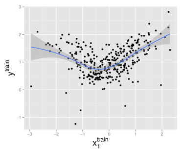
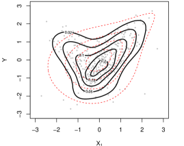
Figure 3: Left: Exemplary scatterplot between $Y$ and $X_{1}$ in the setting $\sigma=0.1$ and $n_{train}=300$ of Scenario M5, together with a locally weighted scatterplot smoothing line. Right: Empirical nonparametric contour plot of the copula between $X_{1}$ and $Y$ with standard normal margins (solid) and the corresponding contour plot of the fitted copula (dashed).

We clearly see a non-monotonic relationship between $X_{1}$ and $Y$. Currently, no pair-copula implemented in the VineCopula package is able to model such a dependence. The solid lines of the right panel of Figure 3 display the empirical nonparametric contour plot of the corresponding copula with standard normal margins generated by the function kdecop of the package kdecopula (Nagler, 2016). In dashed lines the corresponding contour plot of the fitted parametric copula is shown (Joe copula with $\tau\approx 0.25$). The unsatisfying model fit is obvious and explains the rather high estimated MISE values. With this in mind, it is also understandable that a larger training sample size does not help to improve the model fit and prediction accuracy of D-vine quantile regression for this example. However, we observe that the nonparametrically estimated copula manages to model the non-monotonic dependence of the data quite well (for visualization purposes we added the data points transformed to have standard normal margins as well). Hence, by using a nonparametric copula to model the dependence of the pair $(Y,X_{1})$, a model misspecification as described in Dette et al. (2014) would be avoided. Further, as discussed in Nagler and Czado (2016) in detail, by modeling only bivariate copulas nonparametrically the dreaded curse of dimensionality is evaded.

6 Application to the CDS data set

As an application of D-vine quantile regression to real data we want to exploit interdependencies in the financial market in order to set up models that are able to forecast performances of single institutions as well as construct global stress tests. For these purposes we consider a data set containing 1371 daily observations (01/04/2006 – 10/25/2011) of log-returns of credit default swap (CDS) spreads with 5 year maturity of 38 European, US American and Asian-Pacific financial institutions in the banking and insurance sectors. This data set has already been analyzed by Brechmann et al. (2013), who argue that CDS spreads are a viable and accurate measure of a company’s creditworthiness. After applying an appropriate GARCH model to each of the univariate time series in order to get approximately i.i.d. residuals, Brechmann et al. (2013) perform stress tests. By sampling from a conditional C-vine the authors stress one company at a time (i.e. setting it to its 90%/95%/99% quantile) and examine the impact on the other institutions conditioned on this stress event. With our method we can go even further and consider scenarios where more than one company is in distress. This allows us to investigate the spillover effects of a financial crisis in a certain region or branch to other regions and branches. Additional to the stress tests we use D-vine quantile regression models later in this chapter in order to predict an institution’s CDS spread log-returns given its past values and the log-returns of peer companies. In an out-of-sample test we demonstrate the competitiveness of our approach once again.

6.1 Stress testing

The financial institutions considered in the stress test are 18 banks and 20 (re-)insurers from the regions USA, Europe and Asia-Pacific:

• Banks: USA (Goldman Sachs (GS), JP Morgan Chase (JPM), Citigroup), Europe (Banco Bilbao Vizcaya Argentaria (BBVA), Banco Santander (BS), Barclays, BNP Paribas, Deutsche Bank (DB), Intesa Sanpaolo, Royal Bank of Scotland (RBS), Société Générale (SG), Standard Chartered (StanCha), UBS, Unicredit), Asia-Pacific (Bank of China (BoC), Kookmin Bank, Sumitomo Mitsui, Westpac Banking)

• (Re-)Insurers: USA (ACE, Allstate, American International Group (AIG), Chubb, Hartford Financial Services, XL Group), Europe (Aegon, Allianz, Assicurazioni Generali, Aviva, AXA, Hannover Rück (HR), Legal & General (LG), Munich Re (MR), Prudential, SCOR, Swiss Re (SR), Zurich Insurance), Asia-Pacific (Tokio Marine (TM),QBE Insurance)

We consider three stress scenarios, corresponding to crises originating in different sectors, and investigate the resulting spillover effects. For this, we proceed as in Brechmann et al. (2013) and remove serial dependencies from each of the 38 univariate time series by fitting adequate GARCH models. The resulting residuals $r_{j}$, $j=1,\ldots,38$, which are approximately independent and distributed according to their model’s estimated innovations distribution $\hat{F}_{j}$, carry the information about the dependence structure between the institutions. We consider company $j$ to be stressed at level $\kappa\in(0,1)$, if its residual $r_{j}$ takes on the $100\kappa\%$-quantile of its innovation distribution $\hat{F}_{j}$, i.e. $r_{j}=\hat{F}^{-1}_{j}(\kappa)$. This is equivalent to the PIT transformed variable $u_{j}:=\hat{F}_{j}(r_{j})$ taking on value $\kappa$. Likewise, we are interested in the resulting predicted quantile levels of the non-stressed companies. This allows us to directly work on the u-scale and consider the PIT transformed variables $u_{j}:=\hat{F}_{j}(r_{j})$, $j=1,\ldots,38$, and their dependencies.
In Scenario 1, we analyze the effect of stressing the European systemic banks as specified by International Monetary Fund (2009) at different stress levels. Therefore, we stress the banks Banco Santander, Barclays, BNP Paribas, Deutsche Bank, Royal Bank of Scotland, Société Générale, UBS and Unicredit at level $\kappa\in\{0.9,0.95,0.99\}$ (corresponding to moderate, severe and extreme stress scenarios) and use D-vine quantile regression to estimate the conditional medians of the remaining institutions conditioned on this stress event. This way, we can assess the spillover effect to other sectors and regions. The left panel of Figure 4 shows the results of the stress test of Scenario 1. For each institution the predicted median values for the three stress levels are coded by circles (moderate stress with $\kappa=0.9$), diamonds (severe stress with $\kappa=0.95$) and triangles (extreme stress with $\kappa=0.99$). For visualization, the currently stressed institutions’ names are printed in bold and italic. Further, solid lines separate the geographical regions (Europe in the upper, USA in the middle and Asia-Pacific in the lower panel), while dashed lines separate banks (upper) from insurance companies (lower).

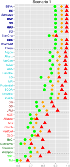
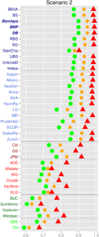
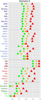
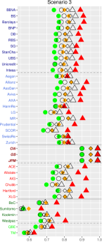
Figure 4: Stress tests stressing European systemic banks (left), major European banks (middle) and US banks (right). For each institution the predicted median values for the three stress levels are represented by circles (moderate stress with $\kappa=0.9$), diamonds (severe stress with $\kappa=0.95$) and triangles (extreme stress with $\kappa=0.99$).

We observe that the spillover effect is strongest for European insurances with predicted median values of up to 0.98 (Allianz and Aviva) for the extreme stress scenario. The comparably small values of the British bank Standard Chartered are explained by the fact that according to their annual report of 2014 (https://www.sc.com/annual-report/2014/documents/SCB_ARA_2014_full_report.pdf) 90% of the bank’s income and profits are earned in Asia, Africa and the Middle East. Similar arguments holds for the British insurance company L&G with operations in Asia and the United States (http://www.legalandgeneralgroup.com/all-our-sites/). Another group that is affected quite strongly by this stress scenario are the US banks with predicted median values exceeding 0.9 in the extreme stress case. However, we observe that the geographic spillover effect is stronger than the institutional one, because the effect on European insurance companies is stronger than the effect on US banks. US insurance companies as well as the Asian-Pacific market are also affected by the stress scenario, but not as severe as the other groups.
It is interesting to see that in Scenario 2, where we only stress the three major European banks Barclays, BNP Paribas and Deutsche Bank, the results of the stress test are very similar to those of Scenario 1. We can conclude, that for a crisis to evolve it suffices that only few but important banks default. In the last scenario, we analyze the spillover effect of a default of the US American banking system (see third panel of Figure 4). Therefore, we stress the banks Citigroup, Goldman Sachs and JP Morgan Chase at level $\kappa\in\{0.9,0.95,0.99\}$ and estimate the conditional medians of the remaining institutions conditioned on this stress event. Again, we see the quite strong interconnectedness between US banks and insurance companies, as well as between US banks and the European market, and observe rather weak spillover effects on the Asian-Pacific sector.
Finally, in the right panel of Figure 4, we compare the stress testing results of D-vine quantile regression to those of linear quantile regression for Scenario 3. Additional to the filled symbols indicating the results of DVQR, we also added the predicted medians of LQR with empty symbols, where circles again denote moderate stress ($\kappa=0.9$), diamonds severe stress ($\kappa=0.95$) and triangles extreme stress ($\kappa=0.99$). We see that for almost all companies linear regression overestimates the moderate stress results and underestimates the extreme ones. This reflects the fact that Gaussian dependence structure implied by linear quantile regression fails to imitate the tail dependence that is typically exhibited by financial data such as these CDS log returns. Another flaw of linear quantile regression observable from the plot is that due to the linearity of the model the median predictions for the three different stress levels seem to always have a similar distance to each other. The predictions of the D-vine based quantile regression appear as much more flexible with some narrower, wider and skewed sets of predictions for the three stress levels. The linear quantile regression results of Scenarios 1 and 2 allow for similar conclusions and are therefore omitted here.

6.2 Out-of-sample quantile prediction

In order to assess the prediction performance of D-vine quantile regression we conduct an out-of-sample test. For this, we consider the raw CDS log-return data (i.e. no time series models were fitted). The goal is to predict the companies’ conditional Value-at-Risk at several time points, i.e. the quantiles of $Y_{t}$ (the CDS log-returns of company $Y$ at time $t$) given its past values $Y_{t-1},\ldots,Y_{t-l}$ (for some lag $l\geq 1$) and the past and current values of its peer companies $\mathbf{X}_{t},\ldots,\mathbf{X}_{t-l}$. In the out-of-sample test, we split the data set at a certain time point into a training data set, based on which we will fit the different quantile regression models, and an evaluation data set used assess the performance of the methods. As a split point we choose the date November 8th, 2010, such that the training data set contains $n_{train}=1121$ observations and the evaluation data set contains $n_{eval}=250$ observations. Note that this sample is not i.i.d. However, since we can assume that it fulfills the strong mixing condition due to low autocorrelations for lags higher than 3 (Hansen, 2008), the approach of estimating the marginals nonparametrically is justified.

One by one, we consider the CDS log-returns of each of the 38 financial institutions as responses. For a fixed response it is not possible to use all of the remaining 37 institutions as predictors since the computational times for the nonparametric and semiparametric quantile regression methods would be too high. Therefore, we reduce the number of predictors by running the D-vine regression algorithm on all of the remaining institutions with lag value $l$ equal to 2 and choosing only the meaningful institutions as potential covariates. This D-vine based screening of the covariates results in a total of 5-10 variables selected, depending on the response institution. No lags higher than $l=1$ were chosen.

Using the selected covariates, for each of the 38 institutions we fit the five previously introduced quantile regression methods on the training data and afterwards apply them to the out-of-sample data set to estimate conditional quantiles at levels $\alpha\in\{0.5,0.01,0.99,0.995\}$. Note that for $\alpha=0.995$ the predicted quantile corresponds to the conditional Value-at-Risk at the $99.5\%$-level.

In this out-of-sample test the true regression quantiles are unknown, we just observe a realization for each day. A possible way of evaluating the predicted $\alpha$-quantiles for some $\alpha\in(0,1)$ is given by the averaged tick-loss $L^{j}_{\alpha,m}$ (see e.g. Komunjer, 2013), which, for company $j$, evaluation sample size $n_{eval}$, observations $y^{(i)}$ and quantiles $q_{\alpha,m}^{(i)}$ predicted by using method $m$, $i=1,\ldots,n_{eval}$, is defined by

$$L^{j}_{\alpha,m}=\frac{1}{n_{eval}}\sum_{i=1}^{n_{eval}}\rho_{\alpha}(y^{(i)}-\hat{q}_{\alpha,m}^{(i)}),$$

where again $\rho_{\alpha}(y)=y(\alpha-\mathbbm{1}(y<0))$ denotes the check or tick function.

Table 7 displays the tick-loss $L_{\alpha,m}$ of predicted quantiles at levels $\alpha\in\{0.5,0.01,0.99,0.995\}$ for the prediction methods $m\in\{\text{DVQR},\text{LQR},\text{BAQR},\text{NPQR},\text{SPQR}\}$, averaged over the 38 financial institutions, i.e. $L_{\alpha,m}=1/38\sum_{j=1}^{38}L^{j}_{\alpha,m}$.

quantile	DVQR	LQR	BAQR	NPQR	SPQR
0.5	6.14	6.12	6.15	7.68	6.14
0.01	0.63	0.99	0.69	0.75	0.61
0.99	0.72	1.11	0.82	0.87	0.71
0.995	0.43	0.73	0.50	0.55	0.43

Table 7: Results of the out-of-sample test predicting the CDS log-returns: tick-loss $L_{\alpha,m}$ of predicted quantiles at levels $\alpha\in\{0.5,0.01,0.99,0.995\}$ for different prediction methods averaged over the 38 financial institutions.

A vast majority of the pair-copulas selected by the algorithm for the estimation of the D-vines were t copulas (which is not surprising for a financial data set). As we have seen in Table 5, linear quantile regression works quite well for predicting the median of such models. This might explain why it manages to slightly outperform all other methods in the conditional 0.5-quantile prediction. Moving away from the median to the more extreme quantiles its lack to describe the fat tails of the t copula become apparent, leaving linear quantile regression far behind all the other methods. Further we can observe, that for this data set the D-vine and semiparametric quantile regression method perform very similar and yield better results than their competitors for the prediction of extreme quantiles. The minimal advantage of SPQR might be explained by the fact that the objective of SPQR is exactly to minimize the above loss function. Boosted additive quantile regression succeeds in improving the linear approach for the quantiles in the tails yielding the third-best results. With as many predictors as 5-10, the nonparametric method already seems to run into the curse of dimensionality and thus produces the worst result for the median prediction and the second worst for the prediction of the quantiles in the tails.

All in all, this real data application has supported the findings of the simulation study of Section 5, that D-vine quantile regression is a reasonable tool for estimating conditional quantiles.

7 Conclusions and further research

A new method to predict conditional quantiles is proposed. We have seen that the usage of the flexible D-vine class facilitates fast and accurate estimation. Analyzing the log returns of the CDS spreads of international banks and insurances we extend the analysis of Brechmann et al. (2013). While they analyze the spillover effects stressing only one institution by simulating from a conditioned C-vine, with our new method we are able to perform stress tests that are conditioned on multiple banks and insurances being in distress. In our analysis we found out that the spillover effect is mainly driven by geography, so that European banks have a greater influence on European insurances than on US American banks. Further, the claim of Brechmann et al. (2013) that US banks have a stronger influence on the international financial market than European banks is not supported by our analysis. Stressing the major European banks had a greater overall impact on the financial system than stressing the US American banks.
Moreover, we have seen that there is still room for future research. With the bivariate pair-copulas implemented in the package VineCopula there is currently no possibility to model non-monotonic dependencies between a response and its predictors as is already pointed out in Dette et al. (2014). A remedy for the resulting issue of possible misspecification is the inclusion of nonparametric pair-copulas in the construction of the D-vine used for quantile regression. A further topic of ongoing research is the implementation of D-vines with mixed discrete and continuous margins as discussed in Stöber et al. (2013) in order to yield quantile regression models allowing for discrete as well as continuous responses and predictors.

Appendix

Appendix A D-vine regression algorithm

Input: pseudo copula data $\mathbf{v}=(v^{(i)})_{i=1,\ldots,n}$, $\mathcal{U}=(u^{(i)}_{j})_{j=1,\ldots,d,\ i=1,\ldots,n}$

1:Initialize global variables:

2:$I_{0}\leftarrow\left\{1,\ldots,d\right\}$

3:$\verb+global.max.cll+\leftarrow-\infty$

4:

5:Step 1:

6:for $j\in I_{0}$ do

7:   Use BiCopSelect to estimate $C_{V,U_{j}}$, the AIC-optimal pair-copula for $(V,U_{j})^{\prime}$ based on the data $(\mathbf{v},\mathbf{u}_{j})$

8:   $\operatorname{cll}_{j}\leftarrow\operatorname{cll}(\hat{c}_{V,U_{j}};\mathbf{v},\mathbf{u}_{j})$

9:end for

10:$l_{1}\leftarrow\operatornamewithlimits{argmax}_{j\in I_{0}}\operatorname{cll}_{j}$

11:Update global variables:

12:$\verb+global.max.cll+\leftarrow\max_{j\in I_{0}}\operatorname{cll}_{j}$

13:$I_{1}\leftarrow I_{0}\backslash l_{1}$

14:

15:Step $k$: (the first tree of the current D-vine with $k-1$ covariates has the order $V$–$U_{l_{1}}$–$\ldots$–$U_{l_{k-1}}$ (see the black graph in Figure 2). $I_{k-1}$ contains the indices of the covariates that have not yet been chosen for the model and global.max.cll is equal to the conditional log-likelihood of the current model)

16:for $j\in I_{k-1}$ do

17:   Estimate $C_{V,U_{j}|U_{l_{1}},\ldots,U_{l_{k-1}}}$ and $C_{U_{l_{i}},U_{j}|U_{l_{i}+1},\ldots,U_{l_{k-1}}}$, $i=1,\ldots,k-1$, i.e. the pair-copulas needed to extend the current D-vine to a D-vine with order $V$–$U_{l_{1}}$–$\ldots$–$U_{l_{k-1}}$–$U_{j}$ (compare Figure 2)

18:   $\operatorname{cll}_{j}\leftarrow\operatorname{cll}(\hat{c}_{V,U_{l_{1}},\ldots,U_{l_{k-1}},U_{j}};\mathbf{v},\mathbf{u}_{l_{1}},\ldots,\mathbf{u}_{l_{k-1}},\mathbf{u}_{j})$

19:end for

20:if $\max_{j\in I_{k-1}}\operatorname{cll}_{j}<\tt{global.max.cll}$  then

21:   return D-vine with order $V$–$U_{l_{1}}$–$\ldots$–$U_{l_{k-1}}$

22:end if

23:$\verb+global.max.cll+\leftarrow\max_{j\in I_{0}}\operatorname{cll}_{j}$

24:$l_{k}\leftarrow\operatornamewithlimits{argmax}_{j\in I_{k-1}}\operatorname{cll}_{j}$

25:$I_{k}\leftarrow I_{k-1}\backslash l_{k}$

26:

27:After step $d$ has been exercised, return D-vine with order $V$–$U_{l_{1}}$–$\ldots$–$U_{l_{d}}$

In lines 5 and 12 of the algorithm, the AIC- and BIC-corrected conditional log-likelihoods may be used instead of the regular $\operatorname{cll}$. In this case all maximum functions have to be replaced by minimum functions.
Regarding the possible pair-copula families to be selected in line 4 of the code, the families currently implemented in the VineCopula package are Gaussian, t*, Clayton, Gumbel, Frank, Joe, BB1*, BB6*, BB7*, BB8* and Tawn* with respective rotations. Families marked with a star are two-parametric, while the others are one-parametric.

Appendix B Analytically derived conditional copula quantiles

B.1 Conditional copula quantile function based on the Gaussian copula

It is a well known fact that the conditional distribution of a multivariate normal distributed random vector again is normally distributed with shifted mean and covariance matrix (Brachinger et al., 1996). Therefore, assuming

$$(Y,X_{1},\ldots,X_{d})\sim N\left((\mu_{Y},\mathbf{\mu_{\mathbf{X}}})^{\prime},\begin{pmatrix}\sigma^{2}_{Y}&\Sigma_{Y,\mathbf{X}}\\ \Sigma_{Y,\mathbf{X}}^{\prime}&\Sigma_{\mathbf{X},\mathbf{X}}\\ \end{pmatrix}\right),$$ (B.15)

the conditional quantile of $Y$ at level $\alpha\in(0,1)$ given $\mathbf{X}=\mathbf{x}$ can be calculated as

$$F^{-1}_{Y|\mathbf{X}}(\alpha|\mathbf{x})=\Phi^{-1}(\alpha;\mu_{c}(\mathbf{x}),\sigma^{2}_{c}),$$

where $\Phi(\cdot;\mu,\sigma^{2})$ denotes the distribution function of a $N(\mu,\sigma^{2})$-distributed random variable and the conditional parameters $\mu_{c}(\mathbf{x})$ and $\sigma^{2}_{c}$ are given as

$$\mu_{c}(\mathbf{x}):=\mu_{Y}+\Sigma_{Y,\mathbf{X}}\Sigma_{\mathbf{X},\mathbf{X}}^{-1}(\mathbf{x}-\mathbf{\mu_{\mathbf{X}}}),$$

and

$$\Sigma_{c}:=\sigma_{Y}^{2}-\Sigma_{Y,\mathbf{X}}\Sigma_{\mathbf{X},\mathbf{X}}^{-1}\Sigma_{Y,\mathbf{X}}^{\prime}.$$

Hence, by inverting Equation (missing) 3.4 the conditional quantile of the Gaussian copula is given as

$$C^{-1}_{V|U_{1},\ldots,U_{d}}(\alpha|u_{1},\ldots,u_{d})=\Phi(\Phi^{-1}(\alpha;\mu_{c}(\mathbf{x}),\sigma^{2}_{c});\mu_{Y},\sigma_{Y}^{2}),$$

where $\mathbf{x}=\left(\Phi^{-1}(u_{1};\mu_{1},\sigma_{1}^{2}),\ldots,\Phi^{-1}(u_{d};\mu_{d},\sigma_{d}^{2})\right)^{\prime}$.

B.2 Conditional copula quantile function based on the Student’s t copula

Similarly, following Kotz and Nadarajah (2004), we know that the conditional distribution of a multivariate t distributed random vector with $\nu$ degrees of freedom again is t distributed with shifted mean, covariance matrix and degrees of freedom. Therefore, with the same partitions of the mean and covariance matrix as in Equation (missing) B.15, the conditional quantile of $Y$ at level $\alpha\in(0,1)$ given $\mathbf{X}=\mathbf{x}$ can be calculated as

$$F^{-1}_{Y|\mathbf{X}}(\alpha|\mathbf{x})=t^{-1}(\alpha;\nu_{c},\mu_{c}(\mathbf{x}),\sigma^{2}_{c}(\mathbf{x})),$$

where $t(\cdot;\nu,\mu,\sigma^{2})$ denotes the distribution function of a $t(\nu,\mu,\sigma^{2})$-distributed random variable and the conditional parameters $\nu_{c}$, $\mu_{c}(\mathbf{x})$ and $\sigma^{2}_{c}(\mathbf{x})$ are given as

$$\nu_{c}:=\nu+d,$$

$$\mu_{c}(\mathbf{x}):=\mu_{Y}+\Sigma_{Y,\mathbf{X}}\Sigma_{\mathbf{X},\mathbf{X}}^{-1}(\mathbf{x}-\mathbf{\mu_{\mathbf{X}}}),$$

and

$$\sigma_{c}(\mathbf{x}):=\frac{\nu+(\mathbf{x}-\mathbf{\mu_{\mathbf{X}}})^{\prime}\Sigma_{\mathbf{X},\mathbf{X}}^{-1}(\mathbf{x}-\mathbf{\mu_{\mathbf{X}}})}{\nu+d}(\sigma_{Y}^{2}-\Sigma_{Y,\mathbf{X}}\Sigma_{\mathbf{X},\mathbf{X}}^{-1}\Sigma_{Y,\mathbf{X}}^{\prime}).$$

Consequently, the conditional quantile of the t copula is given as

$$C^{-1}_{V|U_{1},\ldots,U_{d}}(\alpha|u_{1},\ldots,u_{d})=t(t^{-1}(\alpha;\nu_{c},\mu_{c}(\mathbf{x}),\sigma^{2}_{c}(\mathbf{x}));\nu,\mu_{Y},\sigma_{Y}^{2}),$$

where $\mathbf{x}=\left(t^{-1}(u_{1};\nu,\mu_{1},\sigma_{1}^{2}),\ldots,t^{-1}(u_{d};\nu,\mu_{d},\sigma_{d}^{2})\right)^{\prime}$.

B.3 Conditional copula quantile function based on the two- and three-dimensional Clayton copula

For the bivariate Clayton copula with parameter $\delta>0$ ($C_{U,V}(u,v)=(u^{-\delta}+v^{-\delta}-1)^{\frac{-1}{{\delta}}}$) the conditional quantile can easily be derived by inverting the h-function, yielding

$$C_{V|U}^{-1}(\alpha|u)=\left\{\left(\alpha^{{\frac{-\delta}{1+\delta}}}-1\right){u}^{-\delta}+1\right\}^{\frac{-1}{\delta}}.$$

The conditional quantile function of a three-dimensional Clayton copula with parameter $\delta>0$ ($C_{U,V,W}(u,v,w)=(u^{-\delta}+v^{-\delta}+w^{-\delta}-2)^{-\frac{1}{\delta}}$) is given by

$$C^{-1}_{U|V,W}(\alpha|v,w)=\left\{(\alpha^{-\frac{\delta}{1+2\delta}}-1)(v^{-\delta}+w^{-\delta}-1)+1\right\}^{-\frac{1}{\delta}}.$$

To derive this, let $(U,V,W)$ follow a three-dimensional Clayton copula with parameter $\delta>0$. Then,

$$C_{U,V,W}(u,v,w)=(u^{-\delta}+v^{-\delta}+w^{-\delta}-2)^{-\frac{1}{\delta}}.$$

In order to derive the conditional distribution of $U$ given $V=v$ and $W=w$ we use a version of Equation (missing) 2.2:

$$C_{U|V,W}(u|v,w)=\frac{\partial}{\partial\xi}C_{U,V;W}(C_{U|W}(u|w),\xi;w)\Big{|}_{\xi=C_{V|W}(v|w)}.$$ (B.16)

For the derivation of $C_{U|W}(u|w)$ we use the fact that $C_{U,W}(u,w)=C_{U,V,W}(u,1,w)=(u^{-\delta}+w^{-\delta}-1)^{-\frac{1}{\delta}}$. Hence,

$$C_{U|W}(u|w) =\frac{\partial}{\partial w}C_{U,W}(u,w)=\frac{\partial}{\partial w}(u^{-\delta}+w^{-\delta}-1)^{-\frac{1}{\delta}}$$

$$=(u^{-\delta}+w^{-\delta}-1)^{-\frac{1}{\delta}-1}w^{-\delta-1},$$

and similarly,

$$C_{V|W}(v|w)=(v^{-\delta}+w^{-\delta}-1)^{-\frac{1}{\delta}-1}w^{-\delta-1}.$$

The corresponding inverse functions are given by

$$C^{-1}_{U|W}(u|w)=\left\{w^{-\delta}\left(u^{-\frac{\delta}{1+\delta}}-1\right)+1\right\}^{-\frac{1}{\delta}}$$

and

$$C^{-1}_{V|W}(v|w)=\left\{w^{-\delta}\left(v^{-\frac{\delta}{1+\delta}}-1\right)+1\right\}^{-\frac{1}{\delta}}.$$

Further,

$$C_{U,V|W}(u,v|w)=\frac{\partial}{\partial w}C_{U,V,W}(u,v,w)=(u^{-\delta}+v^{-\delta}+w^{-\delta}-2)^{-\frac{1}{\delta}-1}w^{-\delta-1},$$

and therefore,

$$C_{U,V;W}(u,v;w) =C_{U,V|W}\left(C^{-1}_{U|W}(u|w),C^{-1}_{V|W}(v|w)|w\right)$$

$$=\left\{w^{-\delta}\left(u^{-\frac{\delta}{1+\delta}}-1\right)+1+w^{-\delta}\left(v^{-\frac{\delta}{1+\delta}}-1\right)+1+w^{-\delta}-2\right\}^{-\frac{1}{\delta}-1}w^{-\delta-1}$$

$$=\left\{w^{-\delta}\left(u^{-\frac{\delta}{1+\delta}}+v^{-\frac{\delta}{1+\delta}}-1\right)\right\}^{-\frac{1+\delta}{\delta}}w^{-\delta-1}=\left(u^{-\frac{\delta}{1+\delta}}+v^{-\frac{\delta}{1+\delta}}-1\right)^{-\frac{1+\delta}{\delta}},$$

which is independent of $w$ and is the distribution function of a bivariate Clayton copula with parameter $\frac{\delta}{1+\delta}$.
Now it remains to calculate the differential in Equation (missing) B.16 and plug in the conditional distributions:

$$\frac{\partial}{\partial\xi_{2}}C_{U,V;W}(\xi_{1},\xi_{2};w)=\left(\xi_{1}^{-\frac{\delta}{1+\delta}}+\xi_{2}^{-\frac{\delta}{1+\delta}}-1\right)^{-\frac{1+\delta}{\delta}-1}\xi_{2}^{-\frac{\delta}{1+\delta}-1}.$$

Finally,

$$C_{U|V,W}(u|v,w) =\left\{\left(v^{-\delta}+w^{-\delta}-1\right)w^{\delta}+\left(u^{-\delta}+w^{-\delta}-1\right)w^{\delta}-1\right\}^{-\frac{1+2\delta}{\delta}}$$

$$\quad\cdot\left(v^{-\delta}+w^{-\delta}-1\right)^{\frac{1+\delta}{\delta}\cdot\frac{1+2\delta}{1+\delta}}w^{(-\delta-1)\cdot\frac{-1-2\delta}{1+\delta}}$$

$$=w^{-(1+2\delta)}\left(v^{-\delta}+w^{-\delta}-1+u^{-\delta}+w^{-\delta}-1-w^{-\delta}\right)^{-\frac{1+2\delta}{\delta}}$$

$$\quad\cdot\left(v^{-\delta}+w^{-\delta}-1\right)^{\frac{1+2\delta}{\delta}}w^{1+2\delta}$$

$$=(u^{-\delta}+v^{-\delta}+w^{-\delta}-2)^{-\frac{1+2\delta}{\delta}}\cdot(v^{-\delta}+w^{-\delta}-1)^{\frac{1+2\delta}{\delta}}.$$

Inversion with respect to $u$ gives us the sought after conditional quantile function of a three-dimensional Clayton copula:

$$C^{-1}_{U|V,W}(\alpha|v,w)=\left\{(\alpha^{-\frac{\delta}{1+2\delta}}-1)(v^{-\delta}+w^{-\delta}-1)+1\right\}^{-\frac{1}{\delta}}.$$

A visualization of the conditional median and 95% quantile function of a three-dimensional distribution with underlying Clayton copula with parameter and marginals as specified in Table 2 is given in Figure 5.

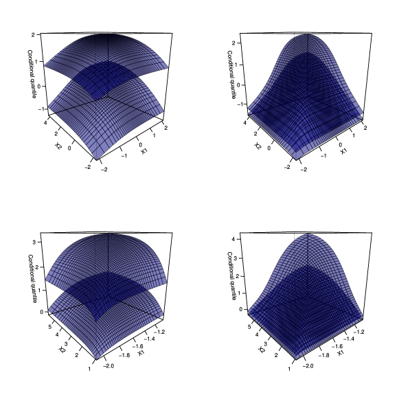
Figure 5: Conditional median and 95% quantile function of a three-dimensional distribution with underlying Clayton copula with parameter $\delta_{1}$ (left panels), $\delta_{2}$ (right panels), and marginals $\mathcal{M}_{1}$ (upper panels), $\mathcal{M}_{2}$ (lower panels) as specified in Table 2.

References

- Aas et al. (2009) Aas, K., Czado, C., Frigessi, A., and Bakken, H. (2009), “Pair-copula constructions of multiple dependence,” Insurance: Mathematics and economics, 44, 182–198.
- Adrian and Brunnermeier (2016) Adrian, T. and Brunnermeier, M. K. (2016), “CoVaR,” American Economic Review, 106, 1705–1741.
- Azzalini (2014) Azzalini, A. with the collaboration of Capitanio, A. (2014), The Skew-Normal and Related Families, Cambridge University Press, IMS Monographs series.
- Bedford and Cooke (2002) Bedford, T. and Cooke, R. M. (2002), “Vines: A new graphical model for dependent random variables,” Annals of Statistics, 30, 1031–1068.
- Bernard and Czado (2015) Bernard, C. and Czado, C. (2015), “Conditional quantiles and tail dependence,” Journal of Multivariate Analysis, 138, 104–126.
- Bouyé and Salmon (2009) Bouyé, E. and Salmon, M. (2009), “Dynamic copula quantile regressions and tail area dynamic dependence in Forex markets,” The European Journal of Finance, 15, 721–750.
- Brachinger et al. (1996) Brachinger, W., Fahrmeir, L., Hamerle, A., and Tutz, G. (1996), Multivariate statistische verfahren, Walter de Gruyter.
- Brechmann et al. (2013) Brechmann, E. C., Hendrich, K., and Czado, C. (2013), “Conditional copula simulation for systemic risk stress testing,” Insurance: Mathematics and Economics, 53, 722–732.
- Brownlees and Engle (2012) Brownlees, C. T. and Engle, R. F. (2012), “Volatility, correlation and tails for systemic risk measurement,” Working Paper, NYU.
- Chen et al. (2009) Chen, X., Koenker, R., and Xiao, Z. (2009), “Copula-based nonlinear quantile autoregression,” The Econometrics Journal, 12, S50–S67.
- Cooke et al. (2015) Cooke, R. M., Joe, H., and Chang, B. (2015), “Vine Regression,” Resources for the Future Discussion Paper, 15–52.
- Czado (2010) Czado, C. (2010), “Pair-copula constructions of multivariate copulas,” in Copula theory and its applications, Springer, pp. 93–109.
- Dette et al. (2014) Dette, H., Van Hecke, R., and Volgushev, S. (2014), “Some comments on copula-based regression,” Journal of the American Statistical Association, 109, 1319–1324.
- Duong (2015) Duong, T. (2015), ks: Kernel Smoothing, version 1.9.4.
- Duong (2016) — (2016), “Non-parametric smoothed estimation of multivariate cumulative distribution and survival functions, and receiver operating characteristic curves,” Journal of the Korean Statistical Society, 45, 33–50.
- Fenske et al. (2012) Fenske, N., Kneib, T., and Hothorn, T. (2012), “Identifying risk factors for severe childhood malnutrition by boosting additive quantile regression,” Journal of the American Statistical Association, 106, 494–510.
- Genest and Favre (2007) Genest, C. and Favre, A.-C. (2007), “Everything you always wanted to know about copula modeling but were afraid to ask,” Journal of hydrologic engineering, 12, 347–368.
- Hansen (2008) Hansen, B. E. (2008), “Uniform convergence rates for kernel estimation with dependent data,” Econometric Theory, 24, 726–748.
- Hayfield et al. (2008) Hayfield, T., Racine, J. S., et al. (2008), “Nonparametric econometrics: The np package,” Journal of statistical software, 27, 1–32.
- Hobæk Haff et al. (2010) Hobæk Haff, I., Aas, K., and Frigessi, A. (2010), “On the simplified pair-copula construction — Simply useful or too simplistic?” Journal of Multivariate Analysis, 101, 1296–1310.
- Hothorn et al. (2015) Hothorn, T., Buehlmann, P., Kneib, T., Schmid, M., and Hofner, B. (2015), mboost: Model-Based Boosting, version 2.5-0.
- Hwang and Shim (2005) Hwang, C. and Shim, J. (2005), “A simple quantile regression via support vector machine,” in Advances in Natural Computation, Springer, pp. 512–520.
- International Monetary Fund (2009) International Monetary Fund (2009), Global Financial Stability Report, Washington DC.
- Joe (1997) Joe, H. (1997), Multivariate models and multivariate dependence concepts, CRC Press.
- Killiches et al. (2016a) Killiches, M., Kraus, D., and Czado, C. (2016a), “Examination and visualisation of the simplifying assumption for vine copulas in three dimensions,” arXiv preprint arXiv:1602.05795, accepted for publication in Australian and New Zealand Journal of Statistics.
- Killiches et al. (2016b) — (2016b), “Model distances for vine copulas in high dimensions,” arXiv preprint arXiv:1510.03671.
- Killiches et al. (2016c) — (2016c), “Using model distances to investigate the simplifying assumption, goodness-of-fit and truncation levels for vine copulas,” arXiv preprint arXiv:1610.08795.
- Koenker (2005) Koenker, R. (2005), Quantile Regression, Cambridge University Press: Cambridge UK.
- Koenker (2011) — (2011), “Additive models for quantile regression: Model selection and confidence bandaids,” Brazilian Journal of Probability and Statistics, 25, 239–262.
- Koenker (2013) — (2013), quantreg: Quantile Regression, version 5.05.