Multilane driven diffusive systems

Abstract

We consider networks made of parallel lanes along which particles hop according to driven diffusive dynamics. The particles also hop transversely from lane to lane, hence indirectly coupling their longitudinal dynamics. We present a general method for constructing the phase diagram of these systems which reveals that in many cases their physics reduce to that of single-lane systems. The reduction to an effective single-lane description legitimizes, for instance, the use of a single TASEP to model the hopping of molecular motors along the many tracks of a single microtubule. Then, we show how, in quasi-2D settings, new phenomena emerge due to the presence of non-zero transverse currents, leading, for instance, to strong ‘shear localisation’ along the network.

1 Introduction

Driven diffusive systems encompass a broad class of statistical physics models involving many interacting particles moving stochastically under dynamics that do not respect detailed balance [1, 2]. As such, the stationary states attained in these systems are nonequilibrium stationary states (NESS) and exhibit currents both at the macroscopic level (particle currents) and microscopic level (probability currents in configuration space).

One-dimensional realisations have proven particularly informative. The general scenario is a one-dimensional lattice connected to particle reservoirs of fixed density at each end. The macroscopic current that flows through the system is determined by an interplay between the boundary reservoir densities and the bulk dynamics of the particles. As pointed out by Krug [3] this can lead to boundary-induced phase transitions, wherein the macroscopic current can be controlled by the boundary rather than bulk dynamics—such transitions have no counterpart in equilibrium stationary states which contain no currents.

The first model of this kind to be studied in detail was the Totally Asymmetric Simple Exclusion Process with open boundaries (TASEP) for which an exact phase diagram was derived [4, 5, 6]. For more general models, however, exact solutions are difficult to come by, therefore to make progress it is important to develop approximations such as mean field theory [4] and heuristic approaches. For one-dimensional models a particularly useful approach uses an Extremal Current Principle (ECP) [3, 7, 8]. The principle (see below) uses the relation $J(\rho)$, between the particle current $J$ and local particle density $\rho$, along with the boundary conditions to derive the phase diagram. Its predictions are borne out by exact phase diagrams, for example in the case of the TASEP.

It is noteworthy that the TASEP had first been introduced some years ago as a model for ribosome dynamics in RNA translation [9]. Since then variants of the basic model have been used as a description of various biophysical transport process such as molecular motors moving on microtubules [10, 11], fungal hyphae growth dynamics [12], extraction of membrane tubes [13] and the model has become a generic starting point to describe transport processes [14, 15]. However, many of these processes require a more complicated geometry than a single one-dimensional lattice. For example, motorway traffic involves several lanes with interchange between lanes and the motion of motor proteins along cytoskeletal filaments often has multiple tracks which may involve different hopping and boundary rates and possibly motors moving in different directions [16, 17]. Pedestrian flows often involve two “multi-lane streets” crossing perpendicularly and a collective dynamics arises in the crossing region [18]. Inspired by these contexts multilane exclusion processes have been considered by several authors [19, 20, 21, 22, 23, 24, 25, 26, 27, 28, 29, 30, 31] (see for example [32] for an overview) and moreover exclusion processes on more complicated graphs such as trees and networks have been formulated and results obtained [33, 34, 35]. However, for these more complicated geometries exact solutions are few and far between, therefore approximate or heuristic approaches are essential.

In [32] a general class of two-lane models has been considered under the main restrictions that: (i) The transport within a lane is local and depends only on the densities within that lane and not on those of neighbouring lanes. (ii) The average transverse flux of particles from one lane to the other increases with the density of the departing lane and decreases with that of the arriving one [32]. Under these conditions it was shown, through a linear stability analysis of the continuum mean-field equations for the densities, how the phase diagram can be constructed. This construction turns out to be equivalent to an ECP which holds for the total particle current $J_{\rm tot}$, defined as the sum of the particle currents in each lane.

In this work we generalize this stability analysis to the multi-lane case which naturally connects one-dimensional lattice gases to their two dimensional counterparts or to more general network topolgies. In addition to the longitudinal currents flowing along each lane, new steady transverse currents flowing between the lanes can be observed in such systems. Their impact on the phenomenology of multi-lane system has not been studied so far. By studying the eigenvalue spectrum of the linearised mean-field equations for the densities, we show how an ECP holds for the total longitudinal current. This result implies that a system with an arbitrary number of lanes (such as the motion of molecular motors along the protofilaments of microtubules) may effectively be described by a one-lane system with generally a non-trivial current density relation, validating an assumption that is commonly made, see for example [36] and references therein. A consequence of this effective description is that the transverse current does not enter into the determination of the phase diagram. Nevertheless, transverse currents can be associated with interesting new phenomena. For instance, one can consider “sheared” systems, in which boundary conditions impose different transverse currents at the two ends of the system. For diffusive bulk dynamics, the transverse current varies continuously, interpolating between its imposed boundary conditions. As we show in this article, for systems driven in the bulk, one may observe a discontinuity in the transverse current corresponding to shear localisation.

The paper is organised as follows. In section 2, for sake of completeness, we review the ECP for the single-lane TASEP. In section 3, we then present the general framework used in this article to describe multi-lane systems: their description at the level of continuum mean field equations. In section 4 we present a linear analysis of these equations and use these results to formulate a general method for constructing phase diagrams, which amounts to a generalised ECP. In section 5, we turn to concrete examples and present numerical simulations of microscopic models. This allows us to confirm our predictions as well as illustrate the new phenomenology associated to steady transverse currents. Technical details and proofs are left to the appendices.

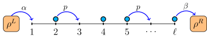
Figure 1: Illustration of the one-dimensional totally asymmetric exclusion process with open boundaries (TASEP)

2 A brief recap of the TASEP

Before turning to the full multilane problem it is useful to recall the TASEP and its phase diagram. The TASEP consists of a one-dimensional lattice of length $\ell$ with totally asymmetric hopping dynamics of hard-core particles: at most one particle is allowed at each site and particles can only move in the forward direction with rate $p$ which we may take to be unity (see fig. 1). At the left boundary particles enter with rate $\alpha$ provided the first site is empty and when a particle arrives at the right boundary it leaves with rate $\beta$. For $\alpha,\beta\leq 1$ these boundary conditions correspond to a left reservoir with density $\rho^{L}=\alpha$ and a right reservoir with density $\rho^{R}=1-\beta$.

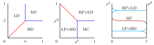
Figure 2: LEFT: Phase diagram of the TASEP where the control parameters are the injection rate $\alpha$ and ejection rate $\beta$ and the phases are Low Density (LD), High Density (HD) and Maximal Current (MC). CENTER: phase diagram where the control parameters are the left and right reservoir densities and the phases are Left Phase (LP), Right Phase (RP) and Maximal Current (MC). In both cases the blue lines represent a second order phase transition while the red lines represent a first order phase transition. RIGHT: profiles corresponding to left, right and maximal current phases.

The phase diagram for the TASEP in the large $\ell$ limit is illustrated in Fig. 2. The different phases that can be observed are:

• a left phase (LP), corresponding to a bulk profile whose density is equal to that of the left reservoir and in which the current is $J=\rho^{L}(1-\rho^{L})$

• a right phase (RP), corresponding to a bulk profile whose density is equal to that of the right reservoir and in which the current is $J=\rho^{R}(1-\rho^{R})$

• a maximal current phase (MC), corresponding to a bulk profile whose density $\rho^{M}=1/2$ in which the current is maximised at $J=1/4$.

Note that historically the Left and Right phases have been referred to as low density (LD) and high density (HD). Here we use a different terminology that is more appropriate to systems that may include further phases.

To determine the bulk density of single lane systems, Krug [3] introduced a maximal current principle which was later generalized to an ECP [8] to describe systems in which the advected current $J(\rho)$ has more than one extrema. In practice, this principle states that, given two reservoir densities $\rho^{L}$ and $\rho^{R}$, the dynamics select a constant plateau whose density $\rho^{B}$ is intermediate between $\rho^{L}$ and $\rho^{R}$, and tends to maximize or minimize the advected current $J(\rho^{B})$:

$$J(\rho^{B})=\left\{\begin{array}[]{lr}\max_{\rho\in[\rho^{R},\rho^{L}]}\ J(\rho)\qquad\text{if}\quad\rho^{L}>\rho^{R}\\ \min_{\rho\in[\rho^{L},\rho^{R}]}\ J(\rho)\qquad\text{if}\quad\rho^{L}<\rho^{R}\;.\\ \end{array}\right.$$ (1)

For the TASEP, the current density relation is $J(\rho)=\rho(1-\rho)$ which is most simply derived from a mean-field consideration that a particle, present with probability $\rho$, moves forward with rate 1 when there is an empty site ahead (which has probability $1-\rho$). The current-density relation for the TASEP has a single extremum which is a maximum of the current at $\rho=1/2$. The ECP then allows one to easily derive the phase diagram shown in Fig 2. Note that for more general current density relations, which may exhibit several extrema, the ECP predicts, in addition to the Left, Right and Maximal Current Phases exhibited by the TASEP, a new minimal current phase (mC). This phase corresponds to a bulk profile whose density $\rho^{m}$ is a local minimum of the current-density relation $J(\rho)$.

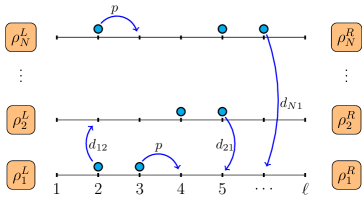
Figure 3: Schematic representation of $N$ parallel TASEPs which are connected at both ends to particle reservoirs of fixed densities. Particles hop along each lane, to the right, at rate $p$ and can hop from lane $i$ to lane $i\pm 1$ at rate $d_{i,i\pm 1}$, giving rise to non-zero longitudinal and transverse currents.

3 General framework

In this article, we consider driven diffusive systems in which particles hop along or between $N$ parallel one-dimensional lattices each of $\ell$ sites. At both ends, each of these $N$ ‘lanes’ is in contact with its own particle reservoir which acts as lattice site of fixed mean density denoted by $\rho_{i}^{L/R}$ for the left/right boundary site of lane $i$. One simple system falling in this class consists of the $N$ parallel TASEPs shown in Fig. 3.

As a starting point of our analysis, we assume that the dynamics of the system is described by a set of $N$ coupled non-linear mean-field equations for the density $\rho_{i}(x,t)$ of particles in lane $i$:

$$\dot{\rho}_{i}(x,t)=-\partial_{x}[J_{i}(\rho_{i}(x,t))-D_{i}\partial_{x}\rho_{i}(x,t)]+\sum_{j\neq i}K_{ji}(\rho_{j}(x,t),\rho_{i}(x,t)),$$ (2)

where $x=n/\ell$ is the position of site $n$ along each lane, $J_{i}(\rho_{i}(x))$ and $-D_{i}\partial_{x}\rho_{i}$ are the advective and the diffusive parts of the mean-field current along lane $i$, and $K_{ji}$ is the net transverse current flowing from lane $j$ to lane $i$ (with $K_{ij}=-K_{ji}$). Throughout this article, we consider systems which satisfy

$$\partial_{\rho_{i}}K_{ij}(\rho_{i},\rho_{j})>0\quad\text{and}\quad\partial_{\rho_{j}}K_{ij}(\rho_{i},\rho_{j})<0\;.$$ (3)

Physically, this means that the net flux of particles from lane $i$ to lane $j$ increases with $\rho_{i}$ and decreases with $\rho_{j}$.

If the hopping rate of particles along lane $i$ depends on the occupancies of lane $j\neq i$, then $J_{i}$ will depend on $\rho_{j}$ and not solely on $\rho_{i}$. In this article, however, we restrict our attention to the case where the hopping rate along one lane depends only on the occupancies of this lane, so that the mean-field longitudinal current depends only on the density of this lane: $J_{i}(\rho_{i})$.

The derivation of (2) from the microscopic dynamics models follows a standard mean-field approximation comprising factorisation of all density correlation functions which we review in section 5. For illustrative purposes we consider the example presented in Fig. 3 of coupled totally asymmetric exclusion processes: particles hop forward longitudinally along the lane $i$ from site $n$ to the next site $n+1$ if that site is vacant with rate $p$; particles can hop transversely to a vacant site at position $n$ in a neighbouring lane $i\pm 1$ with rate $d_{i,i\pm 1}$. Then $J_{i}(\rho_{i})=p\rho_{i}(1-\rho_{i})/\ell$, $D_{i}=p/(2\ell^{2})$ and $K_{i\pm 1,i}=d_{i\pm 1\,,i}\rho_{i\pm 1}(1-\rho_{i})-d_{i,i\pm 1}\rho_{i}(1-\rho_{i\pm 1})$. The explicit form of $J_{i}$, $D_{i}$ and $K_{ij}$ for other models is given in section 5.

Given reservoir densities we want to compute the average density profiles along each lane, i.e. the steady-state solutions of Eq. (2) satisfying $\rho_{i}(0)=\rho_{i}^{L}$ and $\rho_{i}(1)=\rho_{i}^{R}$. Solving this set of $N$ coupled non-linear equations is, however, very hard even in the steady state. Therefore we first consider the possible homogeneous solutions to Eq. (2) which will be valid in the bulk i.e. far from the boundaries. We will refer to these solutions as equilibrated plateaux since their densities are balanced by the exchange of particles between lanes.

As we shall see, these solutions, which we properly define in section 3.1, play a major role in constructing the form of the steady-state profiles and the phase diagrams. We show in section 3.3 how stationary profiles are typically made of equilibrated plateaux connected at their ends either to other plateaux (forming shocks) or directly to the reservoirs, see Fig. 5. For this to hold, the equilibrated plateaux have to be dynamically stable which we show in section 3.2 to be true for systems satisfying conditions (3).

3.1 Plateaux solutions

The plateaux solutions (homogeneous, steady-state solutions denoted $\rho_{i}(x)=\rho_{i}^{\,\rm p}$) are found by setting time and space derivatives to zero in (2). The mean-field steady-state equations then reduce to

$$\forall i\qquad\sum_{j\neq i}K_{ji}(\rho_{j}^{\rm P},\rho_{i}^{\rm P})=0.$$ (4)

Eq. (4) simply states that, for each site of lane $i$, the mean transverse flux of particles coming from all other lanes $j\neq i$ is equal to the mean transverse flux leaving lane $i$.

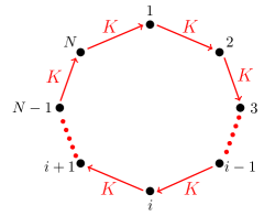
Figure 4: In a system with $N$ parallel lanes, organised on a ring, equilibrated plateaux can be realized with a steady loop of non-zero transverse current $K>0$.

If there are only two lanes, Eq. (4) implies

$$K_{12}=K_{21}=0,$$ (5)

so that there is no net transverse current. However, for a number of lanes $N\geq 3$ the condition (4) can be satisfied by the presence of a non-zero steady loop of transverse current. For example, for $N=3$, with $K_{12}=K_{23}=K_{31}=K\neq 0$, a non-zero steady transverse current is present (see Fig 4 for an illustration with $N$ lanes on a ring).

3.2 Dynamical stability of equilibrated plateaux

The plateaux solutions are only relevant to the steady state if they are dynamically stable. In A we show, through a dynamical linear stability analysis, that a small perturbation $\delta\rho_{i}(x,t)$ around the equilibrated plateau solution:

$$\rho_{i}(x,t)=\rho_{i}^{\,\rm p}+\sum_{q}\delta\rho_{i}^{q}(t)\exp(iqx)\;,$$ (6)

where $q=2\pi n$ with $n=1,\ldots,\ell-1$, vanishes exponentially rapidly in time if one considers systems in which

$$K_{ij}^{i}\equiv\partial_{\rho_{i}}K_{ij}(\rho_{i}^{\,\rm p},\rho_{j}^{\,\rm p})>0\quad\text{and}\quad K_{ij}^{j}\equiv\partial_{\rho_{j}}K_{ij}(\rho_{i}^{\,\rm p},\rho_{j}^{\,\rm p})<0.$$ (7)

Note that this is slightly weaker than condition (3) since (7) only has to hold for equilibrated plateaux densities.

3.3 Equilibrated and non-equilibrated reservoirs

In analogy with equilibrated plateaux, one can define equilibrated reservoirs, whose densities satisfy

$$\forall i\qquad\sum_{j\neq i}K_{ji}(\rho_{j}^{R,L},\rho_{i}^{R,L})=0,$$ (8)

where $\rho_{i}^{L}$ and $\rho_{i}^{R}$ correspond to the densities of the reservoirs at the left and right ends of lane $i$, respectively. If equilibrated reservoirs are imposed at both ends of the system, with $\rho_{i}^{R}=\rho_{i}^{L}$, a simple solution of the mean-field equations in steady state is found by connecting the reservoirs through constant plateaux. Even though these boundary conditions are exceptional, equilibrated plateau solutions play an important role in the steady state of driven diffusive systems. As we show, far from the boundaries, in a large system, the density profile is typically constant. With this in mind, in the following, we will use the term “plateaux” to describe not only completely constant profiles, where the density is the same on all sites of the system, but also flat portions of density profiles, see Fig. 5, which can be connected to reservoirs or other density plateaux by small non-constant boundary layers.

As noted previously, when equilibrated reservoirs are imposed at the two ends of the system with the same densities $\rho_{i}^{L}=\rho_{i}^{R}$, one observes dynamically stable plateaux with $\rho_{i}(x)=\rho_{i}^{L}$. Two other more general classes of boundary condition are relevant.

Figure 5: Example of Left, Right and Shock phases

First, left and right equilibrated reservoirs can imply different sets of plateaux densities in the bulk; how the density is then selected in the bulk is one of the central questions tackled in this article. In Fig. 6, we show examples of Left and Right phases, where the bulk density is controlled respectively by left and right reservoirs. In a left (resp. right) phase, a small modification of the right (resp. left) reservoir densities leaves the bulk part of the density profile unaffected; only the boundary layer connecting to the right (resp. left) reservoir changes.

Second, the reservoirs can be unequilibrated, that is their densities do not obey (8). In this case both left and right reservoir densities are connected to bulk equilibrated plateaux by small boundary layers. In Fig. (7), we show examples of the corresponding left and right phases. Again, in a left (resp. right) phase, a small modification of the right (resp. left) reservoir densities leaves the bulk part of the density profile unaffected; only the boundary layers connecting to the right (resp. left) reservoir changes.

In this article, we focus on how the densities of the equilibrated plateaux in the bulk are selected by the boundary conditions imposed by equilibrated reservoirs and only comment on unequilibrated reservoirs in the conclusion. The boundary layers connecting reservoir to plateaux (or plateaux to other plateaux when a shock is observed as in Fig 5) are beyond the scope of our work, but can be studied using asymptotic methods [37, 30, 39].

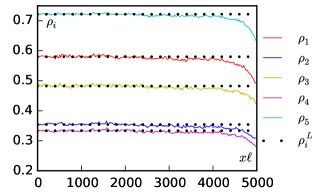
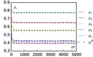
$i$ $\rho_{i}^{L}$ $\rho_{i}^{R}$ 1 0.58 0.45 2 0.35 0.25 3 0.48 0.36 4 0.33 0.24 5 0.72 0.61           $i$ $\rho_{i}^{L}$ $\rho_{i}^{R}$ 1 0.85 0.65 2 0.69 0.42 3 0.79 0.55 4 0.65 0.40 5 0.90 0.77

Figure 6: Connections of equilibrated plateaux to equilibrated reservoirs, for five parallel TASEPs as in Fig. 3. Top and bottom figures correspond to Left and Right phases. Top: The density in the bulk is controlled by the left reservoirs; a small change of the right reservoir densities leaves the bulk plateau unchanged. Bottom: The density in the bulk is controlled by the right reservoirs; a small change of the left reservoir densities leaves the bulk plateau unchanged. For both cases, $p=1$, $d_{12}=10^{-3}$, $d_{23}=9.10^{-3}$, $d_{34}=2.10^{-3}$, $d_{45}=8.10^{-3}$, $d_{51}=3.10^{-3}$, $d_{15}=7.10^{-3}$, $d_{21}=4.10^{-3}$, $d_{32}=6.10^{-3}$, $d_{43}=5.10^{-3}$, $d_{54}=2.10^{-3}$ and results are obtained using continuous time Monte-Carlo simulations.

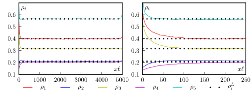
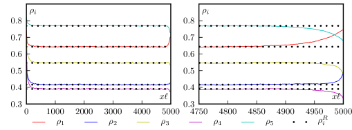
$i$ $\rho_{i}^{L}$ $\rho_{i}^{R}$ 1 0.68 0.45 2 0.15 0.25 3 0.58 0.36 4 0.13 0.24 5 0.92 0.61 $i$ $\rho_{i}^{L}$ $\rho_{i}^{R}$ 1 0.85 0.75 2 0.69 0.52 3 0.79 0.45 4 0.65 0.30 5 0.90 0.67

Figure 7: Connections of equilibrated plateaux to equilibrated and unequilibrated reservoirs, for five parallel TASEPs as in Fig. 3. Top-Left: A bulk plateau is connected to an equilibrated reservoirs on the right and an unequilibrated on the left. This is a left phase and the the bulk density is insensitive to small modification of the density of the right reservoirs. There are thus two boundary layers: one connecting the bulk plateau to the left unequilibrated reservoir, which controls the bulk density, and one connecting the bulk plateau to the right reservoir. Top-Right: Close-up on the unequilibrated left reservoir. Bottom: The same with left equilibrated reservoirs and right unequilibrated reservoirs, in a Right phase. For both cases, $p=1$, $d_{12}=10^{-3}$, $d_{23}=9.10^{-3}$, $d_{34}=2.10^{-3}$, $d_{45}=8.10^{-3}$, $d_{51}=3.10^{-3}$, $d_{15}=7.10^{-3}$, $d_{21}=4.10^{-3}$, $d_{32}=6.10^{-3}$, $d_{43}=5.10^{-3}$, $d_{54}=2.10^{-3}$ and results were obtained using continuous time Monte-Carlo simulations.

4 Phase diagram of multilane systems—a linear analysis

The mean-field dynamics (2) evolves the density profiles towards flat plateaux which are connected at their ends either to other plateaux or to reservoirs. The acceptable plateaux solutions can thus be worked out by considering which types of stationary profiles can connect a bulk plateau to other densities at its right and left ends. For instance, in the bottom panels of Fig. 7, the steady-state solution of the mean-field equations is made up of a plateau connected on its left end to equilibrated reservoirs and on its right end to unequilibrated reservoirs. In practice, we only study whether such profiles can exist by looking at the vicinity of the equilibrated plateau. Namely, rather than solving the full non-linear problem, we carry out a linear analysis of the steady-state mean-field equations

$$0=\partial_{x}[D_{i}\partial_{x}\rho_{i}(x,t)-J_{i}(\rho_{i}(x,t))]+\sum_{j\neq i}K_{ji}(\rho_{j}(x,t),\rho_{i}(x,t)),$$ (9)

around equilibrated plateaux.

We thus look for steady-state profiles of the form

$$|\rho(x))=|\rho^{\,\rm p})+|\delta\rho(x)),\qquad\text{where}\qquad|\rho(x))\equiv\text{\footnotesize $\pmatrix{\rho_{1}(x)\cr\vdots\cr\rho_{N}(x)}$ }$$ (10)

is a compact notation for $N$-dimensional vectors with components $\rho_{i}(x)$ and $|\rho^{\,\rm p})$ corresponds to a set of equilibrated plateau densities. Since we have already established the dynamical stability of equilibrated plateaux in Section 3.2 (and A), we are now only concerned with the existence of spatial stationary perturbations $|\delta\rho(x))$ around them. In the following, we simply refer to $|\delta\rho(x))$ as “perturbations”, omitting their implicit stationarity.

Linearising the steady-state mean-field equations (9) close to $|\rho^{\,\rm p})$ then yields

$$0=D_{i}\partial_{xx}\delta\rho_{i}(x)-J_{i}^{i}(\rho_{i}^{\,\rm p})\partial_{x}\delta\rho_{i}(x)+\sum_{j\neq i}[K_{ji}^{i}\delta\rho_{i}(x)+K_{ji}^{j}\delta\rho_{j}(x)],$$ (11)

where $J_{i}^{i}=\frac{\partial J_{i}(\rho_{i})}{\partial\rho_{i}}$ and $K_{ji}^{i}$, $K_{ij}^{j}$ are defined in (7). Equation (11) can be seen as a first order ordinary differential equation $\partial_{x}|v\rangle=M|v\rangle$, where

$$M(\rho_{1}^{\,\rm p},\dots,\rho_{N}^{\,\rm p})=\left(\begin{array}[]{ccc|ccc}\frac{J^{1}_{1}}{D_{1}}&&&&&\\ &\ddots&&&-M^{K}&\\ &&\frac{J^{N}_{N}}{D_{N}}&&&\\ \hline\cr\frac{1}{D}_{1}&&&&&\\ &\ddots&&&0&\\ &&\frac{1}{D}_{N}&&&\end{array}\right),\;|v\rangle=\text{\footnotesize $\pmatrix{D_{1}\delta\rho_{1}^{\prime}(x)\cr\vdots\cr D_{N}\delta\rho_{N}^{\prime}(x)\cr\delta\rho_{1}(x)\cr\vdots\cr\delta\rho_{N}(x)}$ }$$ (12)

Here, $M^{K}$ is an $N\times N$ matrix defined as

$$M^{K}_{ii}=\sum_{j\neq i}K_{ji}^{i}\qquad M^{K}_{ij}=K_{ji}^{j}\,,$$ (13)

$|v\rangle$ is a compact notation for $2N$-dimensional vectors and $\delta\rho_{i}^{\prime}(x)\equiv\partial_{x}\delta\rho_{i}(x)$. When $M$ is diagonalizable, solutions of this ordinary differential equation are of the form

$$|v(x)\rangle=\sum_{k=0}^{2N-1}\alpha_{k}e^{\lambda_{k}x}|v^{k}\rangle$$ (14)

where $|v^{k}\rangle=(D_{1}\lambda_{k}\delta\rho^{k}_{1},\dots,D_{N}\lambda_{k}\delta\rho^{k}_{N},\delta\rho_{1}^{k},\dots,\delta\rho_{N}^{k})$ are the $2N$ eigenvectors of the matrix $M$ and $\lambda_{k}$ the corresponding eigenvalues. This implies that the perturbation to the density profile (10) may be decomposed as

$$|\delta\rho(x))=\sum_{k=0}^{2N-1}\alpha_{k}e^{\lambda_{k}x}|\delta\rho^{k})\;.$$ (15)

The study of the spectrum of the matrix $M(\rho_{1}^{\,\rm p},\dots,\rho_{N}^{\,\rm p})$ reveals whether given boundary conditions can be connected to a set of bulk plateaux of densities $|\rho^{\,\rm p})$ through appropriate perturbations $|\delta\rho(x))$ (15). This will allow us in section 4.4 to construct the phase diagram.

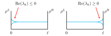
Figure 8: Connecting a reservoir to an equilibrated plateau. With ${\rm Re}(\lambda_{k})\leq 0$, one can construct perturbations connecting an equilibrated plateau to the left reservoirs. With ${\rm Re}(\lambda_{k})\geq 0$, one can construct perturbations connecting an equilibrated plateau to right reservoirs.

We now detail how the spectrum of $M$ is organised and the role played by its eigenvectors. One might expect the study of the spectrum of a $2N$ dimensional matrix to be rather complex. But, as we show below, a simple result for the phase diagram, which is solely determined by the number of eigenvalues with positive (or negative) real part, can be obtained. This can be found using a simple criterion which does not require knowledge of the full spectrum.

Specifically, we show in section 4.1 that there is always one zero eigenvalue, $\lambda_{0}$, whose eigenvector corresponds to a (unique) uniform perturbation which preserves the equilibrated plateau condition. Then, in section 4.2, we show that the rest of the spectrum can be organised in two different ways: Either with $N-1$ eigenvectors with ${\rm Re}(\lambda_{k})<0$ and $N$ with ${\rm Re}(\lambda_{k})>0$, or with $N$ eigenvectors with ${\rm Re}(\lambda_{k})<0$ and $N-1$ with ${\rm Re}(\lambda_{k})>0$. We show that the first case is compatible with a Left Phase and the second with a Right Phase (see Fig. 8) . The separation between these two cases is thus controlled by the change of sign of the real part of an eigenvalue, which we show in section 4.3 to occur at extrema of the total current $J_{\rm tot}$ within the space of equilibrated plateaux.

Sections 4.1 to 4.3 thus establish the possibility, at the linear level, of a non-uniform profile $|\rho(x))$ connecting a plateau $|\rho^{\,p})$ to other equilibrated density vectors at one of its ends. By studying the dynamics of the shocks connecting the plateaux, in section 4.4, we derive a simple recipe for constructing the phase diagram. Readers who are primarily interested in the construction of the phase diagram may thus proceed directly to Sec. 4.4 upon a first reading of this paper.

4.1 Uniform shift of equilibrated plateaux

We now show that the matrix $M$ given in (12) always admits a unique $\lambda_{0}=0$ eigenvalue, associated to uniform shifts of the densities of equilibrated plateaux. Using $M|v^{0}\rangle=0$ implies that $|v^{0}\rangle=(0,\dots,0,\delta\rho_{1}^{0},\dots,\delta\rho_{N}^{0})$ with

$$M^{K}|\delta\rho^{0})=0.$$ (16)

One easily checks that $M^{K}$ is a Markov (or Intensity) matrix by summing its row elements: $\forall j,\;\sum_{i}M^{K}_{ij}=0$. By the Perron-Frobenius theorem $M$ has a unique $\lambda=0$ eigenvector $|\delta\rho^{0})$ which is real and has all its non-zero components of the same sign (which we take to be positive).

It is easy to check that a perturbation of the density vector from $|\rho^{\,\rm p})$ to $|\rho^{\,\rm p})+\epsilon|\delta\rho^{0})$ for small $\epsilon$ indeed results in an equilibrated plateau, since to first order in $\epsilon$

$$\sum_{j\neq i}K_{ji}(\rho_{j}^{\,\rm p}+\epsilon\delta\rho_{j}^{0},\rho_{i}^{\,\rm p}+\epsilon\delta\rho_{i}^{0}) =\sum_{j\neq i}K_{ji}(\rho_{j}^{\,\rm p},\rho_{i}^{\,\rm p})+\epsilon\sum_{j\neq i}K_{ji}^{i}\delta\rho_{i}^{0}+\epsilon\sum_{j\neq i}K_{ji}^{j}\delta\rho_{j}^{0}$$ (17)

$$=0+\epsilon\sum_{j}M_{ij}^{K}\delta\rho^{0}_{j}=0\;,$$

where we used the fact that $\sum_{j\neq i}K_{ji}(\rho_{j}^{\,\rm p},\rho_{i}^{\,\rm p})=0$ since $|\rho^{\,\rm p})$ is equilibrated.

The vector $|\delta\rho^{0})$ is therefore the unique tangent vector to the one-dimensional manifold of equilibrated plateaux: all infinitesimal perturbations $|\delta\rho^{\,\rm p})$ such that $|\rho^{\,\rm p})+|\delta\rho^{\,\rm p})$ remains equilibrated are thus parallel to $|\delta\rho^{\,\rm 0})$. It is important to bear in mind that since $M$ is a function of $|\rho^{\rm p})$, $|\delta\rho^{0})$ also depends on $|\rho^{\,\rm p})$.

4.2 Connecting equilibrated plateaux to reservoirs

In this subsection we consider how a bulk plateau density vector $|\rho^{\,\rm p})$ may be connected by a density profile to equilibrated reservoirs $|\rho^{\,\rm r})$. For the sake of clarity, we focus here on the main results whose detailed derivations are given in B.

First, as noted above, we show in B.1 that in addition to the $\lambda=0$ eigenvalue discussed in the previous subsection, the spectrum of $M$ is composed of either

$(i)$

$N$ eigenvalues with positive real parts and $N-1$ eigenvalues with negative real parts,

$(ii)$

$N{-}1$ eigenvalues with positive real parts and $N$ eigenvalues with negative real parts.

We then show in B.2 that in case $(i)$ the plateau density vector can only be connected to arbitrary equilibrated reservoir densities to the right. Thus, for equilibrated reservoirs, such plateaux can only be observed in a Left Phase—a phase in which the bulk plateaux are controlled by the left reservoirs—with $|\rho^{\,\rm p})=|\rho^{L})$. Conversely, in case $(ii)$ the plateau density vector can only be connected to arbitrary equilibrated reservoir densities to the left. Such plateaux can thus only be observed in a Right Phase.

As the density vector $|\rho^{\,\rm p})$ varies, the transition between the two cases corresponds to the vanishing of an eigenvalue, whose real part will then change sign. Precisely at the transition one then has $N-1$ eigenvalues with ${\rm Re}(\lambda_{k})>0$, $N-1$ eigenvalues with ${\rm Re}(\lambda_{k})<0$ and two zero eigenvalues. Since the eigenspace associated with $\lambda=0$ is of dimension 2 but there is only one $\lambda=0$ eigenvector, the matrix $M$ is then non-diagonalizable. Let us now show that this corresponds to the local extrema of $J_{\rm tot}$ within the space of equilibrated plateaux.

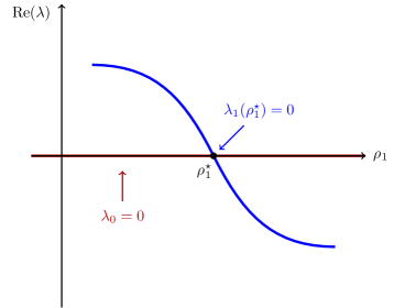
Figure 9: Change of sign of an eigenvalue of stability matrix $M$ given by (12). The eigenvalue $\lambda_{1}$ vanishes at $\rho_{1}=\rho_{1}^{\star}$ while $\lambda_{0}=0$ everywhere.

4.3 Change of sign of ${\rm Re}(\lambda)$ and extrema of the current

From the discussion above it is clear that for the phase diagram to be richer than simply one Left Phase or one Right Phase, we need an eigenvalue, let us denote it $\lambda_{1}$, to vanish and change sign as the reservoir densities are varied.

For equilibrated plateaux $|\rho)$ (to lighten the notation we drop the $\rm p$ superscript), all densities $\rho_{i}$ and all eigenvalues of $M(\rho_{1},\dots,\rho_{N})$ can be written as functions of the density of the first lane $\rho_{1}$ via the equilibrated plateau condition (4). For some value $\rho_{1}^{\star}$, we thus require $\lambda_{1}(\rho_{1}^{\star})=0$ with $\lambda_{1}(\rho_{1}^{\star}\pm\varepsilon)\neq 0$ (see Fig. 9). As we show below, this happens at all the local extrema of the total current

$$J_{\rm tot}(\rho_{1})\equiv\sum_{i}J_{i}[\rho_{i}(\rho_{1})]$$ (18)

within the set of equilibrated plateaux.

At a given plateau $|\rho)$ , the tangent vector to the set of equilibrated plateaux is the $\lambda=0$ eigenvector $|\delta\rho^{0})$ of matrix $M^{K}(\rho_{1},\dots,\rho_{N})$, defined in (13). The extrema of $J_{\rm tot}$ within the set of equilibrated plateaux thus occur when

$$\mbox{d}J_{\rm tot}=\nabla J_{\rm tot}\cdot|\delta\rho^{0})=\sum_{i}J_{i}^{i}\delta\rho^{0}_{i}=0\;.$$ (19)

The linearized steady-state mean-field equation (11) becomes, when we take $\delta\rho_{i}=\delta\rho_{i}^{1}{\rm e}^{\lambda_{1}x}$, an eigenvector equation for $|\delta\rho^{1})$ which reads

$$(\lambda_{1})^{2}D_{i}\delta\rho^{1}_{i}-\lambda_{1}J^{i}_{i}\delta\rho^{1}_{i}+\sum_{j\neq i}(K_{ji}^{i}\delta\rho^{1}_{i}+K_{ji}^{j}\delta\rho^{1}_{j})=0.$$ (20)

By summing (20) over $i$, one finds $(\lambda_{1})^{2}\sum_{i}D_{i}\delta\rho^{1}_{i}-\lambda_{1}\sum_{i}J^{i}_{i}\delta\rho^{1}_{i}=0$ and thus

$$\sum_{i}J_{i}^{i}\delta\rho^{1}_{i}=\lambda_{1}\sum_{i}D_{i}\delta\rho_{i}^{1}.$$ (21)

As we approach $\rho_{1}^{\star}$, where $\lambda_{1}\to 0$, the left hand side of (21) must tend to zero.

However, since $M^{K}$ is a Markov matrix there is a unique eigenvector corresponding to eigenvalue zero which is $|\delta\rho^{0})$. Therefore as $\lambda_{1}\to 0$, we must have $\delta\rho^{1}_{i}\to\delta\rho^{0}_{i}$. Thus as $\rho_{1}\to\rho^{\star}_{1}$ we conclude that

$$\sum_{i}J_{i}^{i}\delta\rho^{1}_{i}\to\sum_{i}J_{i}^{i}\delta\rho^{0}_{i}={\rm d}J_{\rm tot}\to 0.$$ (22)

As $\rho_{1}\to\rho_{1}^{\star}$ this corresponds to the extremal current condition, Eq. (19). The vanishing of ${\rm Re}(\lambda_{1})$ thus occurs at the extrema of $J_{\rm tot}$.

Finally, since $|\delta\rho^{0})$ is the unique zero eigenvector of a Markov matrix $M^{K}$, all its components are of the same sign. As $D_{i}$ are all positive, equations (21) and (22) imply that ${\rm Re}(\lambda_{1}(\rho_{1}))$ and $J^{\prime}_{\rm tot}(\rho_{1})$ are of the same sign in the vicinity of the extrema of $J_{\rm tot}$. Since neither of them vanish and change sign elsewhere, ${\rm Re}(\lambda(\rho_{1}))$ and $J^{\prime}_{\rm tot}(\rho_{1})$ must always have the same sign.

4.4 Phase diagram and extrema of the currents

From sections 4.2 (B) and 4.3, one concludes that for equilibrated plateaux density vectors $|\rho)$, the sign of $J^{\prime}_{\rm tot}(\rho_{1})$ controls the boundary reservoirs to which the plateaux can be connected:

• For $J^{\prime}_{\rm tot}(\rho_{1})>0$, the plateaux can only be connected to different equilibrated densities at their right ends
  

• For $J^{\prime}_{\rm tot}(\rho_{1})<0$, the plateaux can only be connected to different equilibrated densities at their left ends.
  

• $J^{\prime}_{\rm tot}(\rho_{1})=0$ is a singular limiting case between these two regimes;

  • For a local maximum of $J_{\rm tot}$, perturbations with $\delta\rho_{1}>0$ are in a region where $J^{\prime}_{\rm tot}(\rho_{1})<0$ and can thus connect to equilibrated densities with $\tilde{\rho}_{1}>\rho_{1}$ on the left. Perturbations with $\delta\rho_{1}<0$ are in a region where $J^{\prime}_{\rm tot}(\rho_{1})>0$ and can thus connect to equilibrated densities with $\tilde{\rho}_{1}<\rho_{1}$ on the right.

  • For a local minimum of $J_{\rm tot}$, perturbations with $\delta\rho_{1}>0$ are in a region where $J^{\prime}_{\rm tot}(\rho_{1})>0$ and can thus connect to equilibrated densities with $\tilde{\rho}_{1}>\rho_{1}$ on the right. Perturbations with $\delta\rho_{1}<0$ are in a region where $J^{\prime}_{\rm tot}(\rho_{1})<0$ and can thus connect to equilibrated densities with $\tilde{\rho}_{1}<\rho_{1}$ on the left.

  The exact shape of the profile in this case, which may involve algebraic functions rather than exponential, is beyond the scope of this paper.

To construct the phase diagram, one thus computes $J_{\rm tot}(\rho_{1})$ and find the values of all its extrema, as shown in the left panel of Fig. 10. This allows one to determine for each plateau if, and how, it can be connected to other equilibrated densities at its left or right ends, as shown in the central panel of Fig. 10. Then, for given sets of equilibrated reservoirs $|\rho^{L})$ and $|\rho^{R})$, one can construct the profiles which are in agreement with the linear analysis. As shown in the right panel of Fig. 10, these profiles are monotonous and made of successions of plateaux, whose densities are set by the reservoirs or correspond to local extrema of the current, connected by shocks.

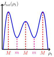
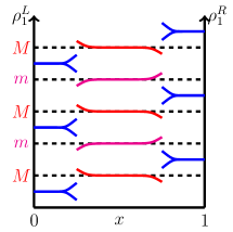
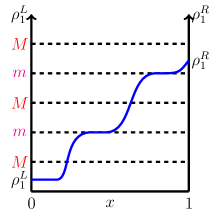
Figure 10: Left: Example of current density relation $J_{\rm tot}(\rho_{1})$. Center: Linear stability of all equilibrated plateau. Right: Example of possible profiles connecting left and right reservoirs. The shocks connecting the plateaux need not be stationary.

While such shocks are in agreement with the linear analysis of the steady-state mean-field equations, they need not be stationary. Let us consider the situation depicted in Fig. 11. The rate of change of the number of particles in the region $[x_{1},x_{2}]$ due to the moving shock profile is

$$\dot{\cal N}_{[x_{1},x_{2}]}=v\sum_{i}(\rho_{i}^{1}-\rho^{2}_{i})\;,$$ (23)

where $v$ is the shock velocity and the sum is over lanes. By the continuity equation for the number of particles the rate of change is also given by the fluxes at the boundary of the region, thus

$$\dot{\cal N}_{[x_{1},x_{2}]}=\int_{x_{1}}^{x_{2}}\sum_{i}\dot{\rho}_{i}=\sum_{i}\left[J_{i}(\rho^{1}_{i})-J_{i}(\rho_{i}^{2})\right]$$ (24)

Equating the two expressions, the velocity $v$ of the shock is thus given by

$$v=\frac{J_{\rm tot}(\rho^{1}_{1})-J_{\rm tot}(\rho^{2}_{1})}{\rho^{1}_{\rm tot}-\rho^{2}_{\rm tot}}$$ (25)

where $\rho_{\rm tot}=\sum_{i}\rho_{i}$.

Let us now show that the sign of $\rho^{1}_{\rm tot}-\rho^{2}_{\rm tot}$ is the same as the sign of $\rho^{1}_{1}-\rho^{2}_{1}$. Since the tangent vector to the set of equilibrated plateau, $|\delta\rho^{0})$, has all its components of the same sign, a small increase in $\rho_{1}$ results in a new equilibrated plateau with small increases of $\rho_{i\neq 1}$. The total density $\rho_{\rm tot}$ is thus an increasing function of $\rho_{1}$: if one has $\rho_{1}^{1}<\rho_{1}^{2}$ (resp. $\rho_{1}^{1}>\rho_{1}^{2}$) then one must have $\rho_{\rm tot}^{1}<\rho_{\rm tot}^{2}$ (resp. $\rho_{\rm tot}^{1}>\rho_{\rm tot}^{2}$). Increasing and decreasing shocks thus correspond to $\rho^{2}_{1}>\rho^{1}_{1}$ and $\rho^{2}_{1}<\rho^{1}_{1}$.

Increasing shocks thus move to the right if $J_{\rm tot}(\rho_{1})<J_{\rm tot}(\rho_{2})$ and the plateau of density $\rho_{1}$ invades the plateau of density $\rho_{2}$. Conversely if $J_{\rm tot}(\rho_{1})>J_{\rm tot}(\rho_{2})$, the shock moves to the left and the plateau of density $\rho_{2}$ widens. For decreasing shocks, on the the other hand, the plateau corresponding to the larger current widens.

Note that the shocks on all lanes are co-localized, as shown by our linear stability analysis. Intuitively, unequilibrated densities would otherwise have to coexist between, say, the shock on lane $1$ and on lane $2$, which would make the profiles unstable [29].

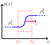
Figure 11: Schematic of a shock profile connecting a plateau of density $\rho_{1}^{1}$ to a plateau of density $\rho_{1}^{2}$ moving with speed $v$. The number of particles within the red rectangle varies at a rate $v(\rho^{1}_{\rm tot}-\rho^{2}_{\rm tot})$. If $v>0$ the plateau at $\rho_{1}=\rho_{1}^{1}$ spreads while the plateau at $\rho_{1}=\rho_{1}^{2}$ recedes. Conversely, for $v<0$, the plateau at $\rho_{1}=\rho_{1}^{2}$ spreads while the one at $\rho_{1}=\rho_{1}^{1}$ recedes.

4.4.1 Construction of the phase diagram

We can now gather everything together in a simple rule for constructing the phase diagram:

• For increasing profiles, when $\rho_{1}^{L}<\rho_{1}^{R}$, among all the plateaux in agreement with the linear analysis, the one corresponding to the smallest current spreads while the others recedes. The possible plateaux correspond either to the reservoir densities, if $J^{\prime}_{\rm tot}(\rho_{1})^{L}>0$ or $J^{\prime}_{\rm tot}(\rho_{1})^{R}<0$, or to local minima of the currents (local maxima correspond to decreasing profiles as shown in Fig. 10). For continuous $J_{\rm tot}(\rho_{1})$, the global extrema of $J_{\rm tot}$ on $[\rho^{L},\rho^{R}]$ are either at the boundaries or at local extrema so that the minima of $J_{\rm tot}$ among the possible plateaux correspond to the global minima of $J_{\rm tot}$ on $[\rho_{1}^{L},\rho_{1}^{R}]$. Note that if there are several minima with the same value of the current, a shock connecting these densities does not propagate ballistically but simply diffuses.
  

• For decreasing profiles, when $\rho_{1}^{L}>\rho_{1}^{R}$, the converse reasoning leads to the selection of the plateau(x) with the largest current.
  This is summarized in the generalized ECP discussed in section 4.4.2.

4.4.2 A generalized extremal current principle

Let us now show how our approach relates to the extremal current principle. As noted in Sec. 2, based on the assumption that there exists a relation $J(\rho)$ between the particle current $J$ and local density $\rho$, an extremal current principle can be used to derive the phase diagram of the TASEP [3]. In [32], this principle was generalized to two-lane systems with equilibrated reservoirs by extremising the total current summed over the two lanes. The results of the previous section thus generalizes this approach to the $N$-lane case in the presence of transverse currents.

Given two sets of equilibrated reservoirs at the left and right ends of the system, section 4.4.1 shows the equilibrated densities $\rho_{i}^{B}$ observed in the bulk to satisfy

$$J_{\rm tot}(\rho_{1}^{B})=\left\{\begin{array}[]{lr}\max_{\rho_{1}^{B}\in[\rho_{1}^{R},\rho_{1}^{L}]}\ J_{\rm tot}(\rho^{B}_{1})\qquad\text{for}\quad\rho_{1}^{L}>\rho_{1}^{R}\\ \min_{\rho^{B}_{1}\in[\rho_{1}^{L},\rho_{1}^{R}]}\ J_{\rm tot}(\rho^{B}_{1})\qquad\text{for}\quad\rho_{1}^{L}<\rho_{1}^{R}\;.\\ \end{array}\right.$$ (26)

Note that the $N=2$ case is rather atypical in that $K=0$ automatically, the only non-zero stationary currents are thus longitudinal. For $N>2$, non-zero transverse currents are generically present and it is perhaps surprising that they do not affect the extremal current principle.

5 Microscopic models of multilane systems

In the previous section we presented a linear stability analysis that allowed us to predict the phase diagrams of multilane systems starting from their hydrodynamic descriptions. We now compare our theoretical predictions to various microscopic models. In particular, we discuss the validity of the generalised extremal current principle (26).

We consider $N$ parallel lanes organised transversely “on a ring”, as in Fig. 4: particles can hop from lane $i$ to lane $i\pm 1$, with periodic boundary conditions. This will allow us to study the phenomenology of non-zero transverse currents. We first consider $N=10$ parallel TASEPs in section 5.1 before turning to a partial exclusion processes in section 5.2. Finally, in section 5.4 we discuss a case where, while the simple mean-field approximation we employ is not exact, the generalized extremal current principle still holds.

5.1 $N$ TASEPs on a ring

We consider a system of length $\ell$ composed of $N$ one-dimensional TASEPs. Particles hop along each lane at constant rates and there can be only one particle per site. Each lane is connected to reservoirs at its ends and particles can hop from lane $i$ to the neighbouring lanes $i\pm 1$, giving rise to transverse currents between the lanes. For example, this could mimic the structure of microtubules which are composed of several protofilaments along and between which molecular motors can walk. Previously the case $N=2$ has been considered (see for instance [32] and references therein) whereas the $N=3$ case (without periodic boundary conditions in the transverse direction) has been studied numerically [31]. Here we show that indeed the system of $N$ TASEPs for arbitrary $N$ may be determined by the generalized ECP based on the total current.

A particle on lane $i$ at site $j$ can hop to the neighbouring site $j+1$ of lane $i$ with rate $p_{i}$ and on the site $j$ of lanes $i\pm 1$ with rate $d_{i,i\pm 1}$, provided the arrival site is empty. The microscopic mean-field equations, within the approximation of factorising all density correlation functions, describing these $N$ parallel TASEPs read

$$\frac{\mathrm{d}\rho_{i,j}}{\mathrm{d}t} =p_{i}\,\rho_{i,j-1}(1-\rho_{i,j})-p_{i}\,\rho_{i,j}(1-\rho_{i,j+1})$$ (27)

$$\quad+d_{i-1,i}\,\rho_{i-1,j}(1-\rho_{i,j})-d_{i,i-1}\,\rho_{i,j}(1-\rho_{i-1,j})$$

$$\quad+d_{i+1,i}\,\rho_{i+1,j}(1-\rho_{i,j})-d_{i,i+1}\,\rho_{i,j}(1-\rho_{i+1,j})$$

where $\rho_{i,j}=\langle n_{i,j}\rangle$ is the mean occupancy of the site $j$ of lane $i$ and we use transverse periodic boundary conditions by identifying lanes $i=N+1$ and $i=1$.

We can now define the mean-field currents of the microscopic models:

$${\cal J}_{ij}=p_{i}\,\rho_{i,j}(1-\rho_{i,j+1})$$ (28)

$${\cal K}_{(i,i+1)j}=d_{i,i+1}\,\rho_{i,j}(1-\rho_{i+1,j})-d_{i+1,i}\rho_{i+1,j}(1-\rho_{ij}).$$ (29)

where ${\cal J}_{ij}$ is the mean-field approximation of the ‘longitudinal’ particle current between sites $j$ and $j+1$ of lane $i$ and ${\cal K}_{(i,i+1)j}$ is the mean-field approximation of the ‘transverse’ particle current between sites $j$ of lanes $i$ and $i+1$.

To obtain coarse-grained equations, we introduce the rescaled position $x=j/\ell$ along the lattices which now goes from $x=0$ to $x=1$. One then uses a standard Taylor expansion assuming that $\rho_{i,j}$ varies slowly from site to site along a given lane:

$$\rho_{i,j\pm 1}\equiv\rho_{i}(x\pm\frac{1}{\ell})\simeq\rho_{i}(x)\pm\frac{1}{\ell}\frac{\partial\rho_{i}(x)}{\partial x}+\frac{1}{2\ell^{2}}\frac{\partial^{2}\rho_{i}(x)}{\partial x^{2}}.$$ (30)

By keeping terms up to second order in gradients one can then write the coarse-grained mean-field equations:

$$\dot{\rho}_{i}(x)= -\partial_{x}[J_{i}(\rho_{i}(x))-D_{i}\partial_{x}\rho_{i}(x)]+$$ (31)

$$+K_{i-1,i}[\rho_{i-1}(x),\rho_{i}(x)]-K_{i,i+1}[\rho_{i}(x),\rho_{i+1}(x)]$$

where

$$J_{i}(\rho_{i}(x))=\frac{p_{i}}{\ell}\rho_{i}(x)[1-\rho_{i}(x)],\quad\text{and}\quad-D_{i}\partial_{x}\rho_{i}=-\frac{p_{i}}{2\ell^{2}}\partial_{x}\rho_{i}$$ (32)

are the advective and the diffusive parts of the mean-field current along lane $i$. We stress again that in the models we consider the longitudinal current of one lane depends solely on the occupancies in that lane. $K_{i,i+1}$ is the transverse current from lane $i$ to lane $i+1$ defined as

$$K_{i,i+1}[\rho_{i}(x),\rho_{i+1}(x)]=d_{i,i+1}\rho_{i}(x)[1-\rho_{i+1}(x)]-d_{i+1,i}\rho_{i+1}(x)[1-\rho_{i}(x)],$$ (33)

with $K_{i,i+1}=-K_{i+1,i}$. In steady state, the equilibrated plateau (4) condition then reads

$$\forall i,\qquad K_{i,i+1}=-K_{i+1,i}=K$$ (34)

where periodic boundary conditions are implicit. At this stage, Eqs (31), (32), and (33) completely define the hydrodynamic mean-field description of our model.

We will proceed as follows: We first consider left and right equilibrated reservoirs of equal densities $\rho_{1}^{R}=\rho_{1}^{L}=\rho_{1}$; for each value of $\rho_{1}$, which is an input parameter, we solve the equilibrated mean-field equations (4) to obtain $\rho_{i\neq 1}^{L/R}(\rho_{1})$, $K(\rho_{1})$ and $J_{\rm tot}(\rho_{1})$, which we then use to predict the phase diagram. Let us first compare these mean-field predictions with the result of microscopic Monte-Carlo simulations.

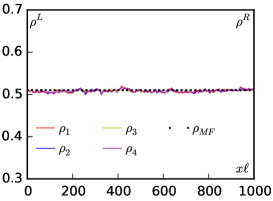
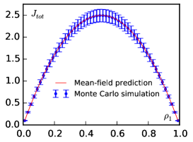
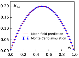
Figure 12: Simulation results for $N=10$ TASEPs on a ring, with $p_{i}=1$ for all lanes and transverse rates: $d_{i,i+1}=0.9$ and $d_{i+1,i}=0.1$. Left: All density profiles are equal and coincide with the mean-field predictions. For sake of clarity, only the densities of lanes 1 to 4 are shown. ($\rho_{1}^{L}=\rho_{1}^{R}=0.51$) Center: the total longitudinal current as a function of $\rho_{1}$; the maximum is at $\rho_{1}^{M}=0.5$. Right: The transverse current between lane 1 and 2 corresponds to its mean-field description. As expected, all other currents $K_{i,i+1}$ are equal to $K_{1,2}$.

We show in Fig. 12 the results of simulations for $N=10$ TASEPs on a ring, with $p_{i}=1$ for all lanes and transverse rates: $d_{i,i+1}=0.9$ and $d_{i+1,i}=0.1$. For such transverse rates, the equilibrated plateau condition simply forces the densities of all lanes to be equal. As predicted, we observe plateau profiles of densities $\rho_{i}(x)\simeq\rho_{i}^{L}=\rho_{i}^{R}$. The currents $J(\rho_{1})$ and $K(\rho_{1})$ are in agreement with their mean-field predictions. We can now use the generalised extremal current principle to construct the phase diagram of the system.

We proceed as in section 4.4: we first identify the extrema of the current and the regions where equilibrated plateaux can be connected to equilibrated reservoirs at different densities on their left or right ends (see the left panel of Fig. 13). We then use the extremal current principle to construct the phase diagram. As show in the right panel of Fig. 13, the agreement between the predicted phase diagram and the results of numerical simulations is very good.

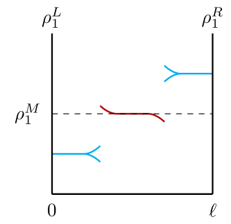
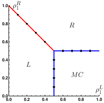
Figure 13: Phase diagram for $N=10$ TASEPs on a ring, with $p_{i}=1$ for all lanes and transverse rates $d_{i,i+1}=0.9$ and $d_{i+1,i}=0.1$. Left: possible connections of equilibrated plateaux predicted by the linear stability analysis. Right: phase diagram where blue lines indicate second order phase transitions and the red line indicates a first order phase transition. Black error bars indicate the phase boundaries obtained by Monte Carlo simulations. The different phases are left (L), right (R) and maximal current phase (MC).

The phase diagram shown in Fig. 13 is identical to that of a single TASEP. This shows that the frequently made assumption that the motion of molecular motors along a microtubule can be modelled by a single TASEP is indeed valid [11, 13]. Note, however, that the transverse current $K$ is generically non-zero along the system (it follows the form of the longitudinal current $J$). Non-zero transverse currents have been observed experimentally, for instance for molecular motors that have helical trajectories along microtubules [44, 45, 46]. Our analysis thus covers the collective dynamics of such motors, suggesting that their propensity to form traffic jams should be identical to that of more standard motors [13, 47].

For the particular choice of rates made in this section, the equilibrated densities are equal across all lanes. The system thus has a particle-hole symmetry, and both $J(\rho_{1})$ and $K(\rho_{1})$ are symmetric with respect to $\rho_{1}=0.5$ (see right panels of Fig. 12). On the first-order transition line (see Fig. 13), $K$ is therefore the same on both sides of a shock. We now turn to a more general system where this symmetry is violated and show that one can have coexistence between plateaux with very different values of the transverse current $K$.

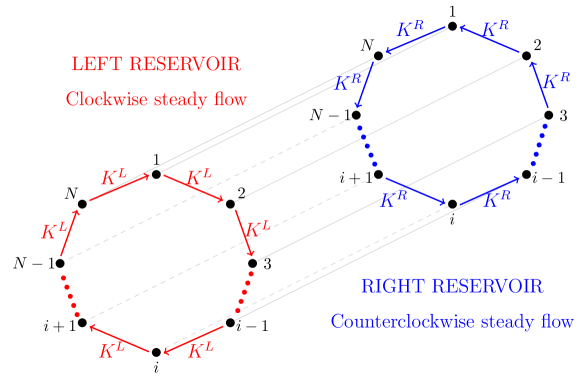
Figure 14: Sketch of a system where $K(\rho^{L})$ is positive and $K(\rho^{R})$ is negative.

5.2 Counter-rotating shocks

Let us now turn to more intriguing cases where the transverse current is not simply proportional to the longitudinal current. A particular example we consider is that of a transverse current which changes sign along the lane. A way of achieving a spatial reversal of $K$ would be to have a transverse current $K(\rho)$ which changes sign as a function of density. Specifically, one could impose reservoir densities at the two ends of the system to have, say, clockwise and counter-clockwise flows imposed by the left and right reservoirs, respectively (see Fig. 14). Thus, at the boundaries the transverse currents have opposite signs. One can then wonder how the transverse flow in the bulk is selected when the system is “sheared” by such boundary conditions.

In order to achieve a transverse current $K(\rho)$ which changes sign as a function of density, one can first relax the condition that the transverse rates $d_{i,i+1}$ and $d_{i,i-1}$ are equal for all lanes. As we show in section 5.4, the equilibration condition then does not impose equal densities on all lanes. The transverse current $K$ generically loses its particle-hole symmetry but, as we show in C, it cannot change sign as a function of density for transverse rates of the form $d_{i,i\pm 1}\rho_{i}(1-\rho_{i\pm 1})$.

As we now show, a partial exclusion process, in which the restriction to at most one particle per site is relaxed, allows us to obtain the desired change of sign in the transverse current Specifically, we study $N$ parallel one-dimensional lattice gases in which up to $N_{\rm max}$ particles are allowed on each site. Particles hop from site $j$ to $j+1$ on lane $i$ with rate

$$W(i,j\to i,j+1)=p_{i}\frac{n_{i,j}}{N_{\rm max}}\left(1-\frac{n_{i,j+1}}{N_{\rm max}}\right)\;$$ (35)

and we refer to this as the Totally Asymmetric Partial Exclusion Process (TAPEP). For the transverse hopping rates from site $j$ of lane $i$ to site $j$ of lane $i\pm 1$, we choose

$$W(i,j\to i\pm 1,j)=d_{i,i\pm 1}\frac{n_{i,j}}{N_{\rm max}}\left(1-\frac{n_{i\pm 1,j}}{N_{\rm max}}\right)$$ (36)

apart from the hopping from lane 1 to 2, in which we impose a different hopping rate

$$W(2,j\to 1,j)=d_{2,1}\left(\frac{n_{2,j}}{N_{\rm max}}\right)^{2}\left(1-\frac{n_{1,j}}{N_{\rm max}}\right)\;.$$ (37)

Note that in the case of the TASEP ($N_{\rm max}=1$) the hopping dynamics from lane 1 to 2 is the same as that between other lanes since $n_{2,j}^{2}=n_{2j}$. Therefore we need to consider partial exclusion ($N_{\rm max}>1$) to observe novel behaviour.

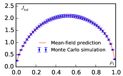
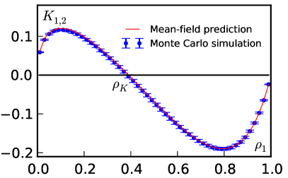
Figure 15: Comparison of numerical simulations of 10 TAPEPs with mean-field predictions. Left: total longitudinal current as a function of $\rho_{1}$: the maximum is at $\rho_{1}^{M}=0.52$. Right: transverse current between lane 1 and 2 (currents between all other pairs of lanes are the same). In the simulation we have set $N_{\text{max}}$=100 and $p=1$ for all the lanes. The transverse rates are: $d_{1,2}=56$, $d_{2,3}=89$, $d_{3,4}=7$, $d_{4,5}=27$, $d_{5,6}=49$, $d_{6,7}=45$, $d_{7,8}=18$, $d_{8,9}=8$, $d_{9,10}=50$, $d_{10,1}=62$, $d_{1,10}=47$, $d_{2,1}=78$, $d_{3,2}=95$, $d_{4,3}=94$, $d_{5,4}=10$, $d_{6,5}=41$, $d_{7,6}=8$, $d_{8,7}=15$, $d_{9,8}=15$, $d_{10,9}=79$.

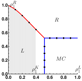
Figure 16: Phase diagram of $N=10$ TAPEPs with $N_{\text{max}}=100$. Left: possible connections of equilibrated plateaux predicted by the linear stability analysis. Right: phase diagram where blue lines indicate second order phase transitions and the red line indicates first order phase transitions. The different phases are left, right or maximal current phases. The gray shaded region corresponds to the region where $K>0$ is observed in the bulk (bottom-left); in the rest of the phase diagram, one observes $K<0$ in the bulk. The rates are the same as in Fig 15.

To derive the hydrodynamic mean-field description of our model, we proceed as before, to obtain a dynamics given by (31), where we have introduced the mean densities

$$\rho_{i,j}=\frac{\langle n_{i,j}\rangle}{N_{\rm max}}\;.$$ (38)

Advective and transverse currents are again given by (32) and  (33), apart from $K_{1,2}$ whose expression is:

$$K_{1,2}=d_{1,2}\rho_{1}(1-\rho_{2})-d_{2,1}(\rho_{2})^{2}(1-\rho_{1}).$$ (39)

Using the methodology introduced in section 4.4, we can now compute, for equilibrated plateaux, the transverse and longitudinal currents $K(\rho_{1})$ and $J_{\rm tot}(\rho_{1})$.

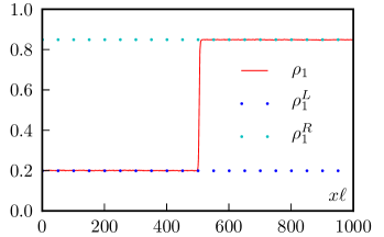
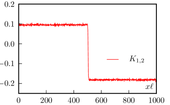
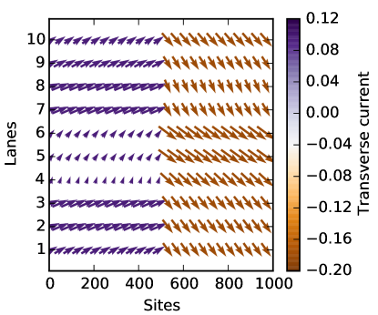
Figure 17: Simulations of $N=10$ TAPEPs with up to $N_{\text{max}}=100$ particles allowed per site. All longitudinal rates are equal ($p_{i}=p=1$) whereas the transverse rates are chosen as follows: $d_{12}=56$, $d_{21}=47$, $d_{23}=89$, $d_{32}=78$, $d_{34}=7$, $d_{43}=95$, $d_{45}=27$, $d_{54}=94$, $d_{56}=49$, $d_{65}=10$, $d_{67}=45$, $d_{76}=41$, $d_{78}=18$, $d_{87}=8$, $d_{89}=8$, $d_{98}=15$, $d_{9\,10}=50$, $d_{10\,9}=15$, $d_{10\,1}=62$, $d_{1\,10}=79$. Top-left: the density profile of lane 1 exhibits a shock between a left and a right phase. The densities imposed at the two reservoirs are $\rho_{1}^{L}=0.199$ and $\rho_{1}^{R}=0.849$. Top-right: The transverse current between lane 1 and 2 similarly shows a shock between two values of opposite signs. Bottom: Vector field of the current $(J_{i},K_{i,i+1})$ along the lattice. The color code shows the value of $K$. The length of the arrows corresponds to the modulus of the current vector.

In Fig. 15, we compare the results of numerical simulations of 10 TAPEPs with mean-field predictions. Again, the agreement is excellent. Significantly, for the particular choice of transverse rate (37), $K(\rho_{1})$ changes sign as $\rho_{1}$ varies, at $\rho_{1}\equiv\rho_{1}^{K}$. Using the expression of $J_{\rm tot}(\rho_{1})$ and the generalised extremal current principle, we derive the phase diagram which is compared with Monte-Carlo simulations in Fig. 16.

On the the red line of Fig. 16, one observes coexistence between two profiles of different densities separated by a shock. On this line, for $\rho^{L}<\rho_{1}^{K}$, these shocks separate the bulk of the system into homogeneous phases with counter-rotating transverse currents (see Fig. 17).

5.3 Shear localisation

The phenomenology shown in Fig. 17 is rather counterintuitive. Indeed, for a Symmetric Partial Exclusion Process which yields diffusive dynamics, one expects the density profile to linearly interpolate between the two reservoir densities. This in turn leads to a continuous variation of the transverse current $K$ (See Fig. 18). In contrast, for the driven-diffusive dynamics of the TAPEP, which leads to the formation of shocks, our analysis shows that a localized discontinuity of the transverse current may occur. Thus in the type of driven system we consider, it is the driven longitudinal dynamics which determine the phase behaviour and the transverse currents are dictated by the longitudinal ones.

For standard fluids, where momentum is conserved, such a shear discontinuity is unexpected [48]. Multilane models, based on random particle hopping, however describe situations where the momentum of the system is not even locally conserved. This is relevant, for instance, to models of molecular motors hopping along a microtubule without a proper description of the surrounding fluid. The shear localization phenomenon thus belongs to the class of surprising phenomena which can be observed in momemtum non-conserving systems (see [49] for how the concept of pressure can fail for such systems).

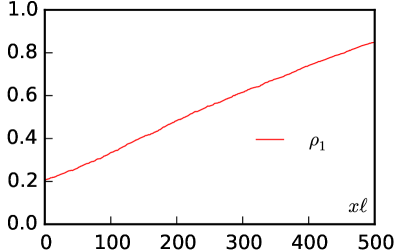
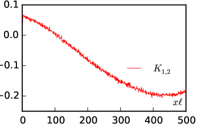
Figure 18: Simulations of 10 Symmetric Partial Exlusion Processes. The simulation details are the same as in Fig. 17 with the exception of the longitudinal dynamics which is now symmetric, i.e. $p=q=1$ for all lanes, where $p$ and $q$ are the forward and backward hopping parameters respectively. Left: density profile of lane 1 linearly interpolates between the left and right boundary conditions. The density values imposed at the two reservoirs are $\rho_{1}^{L}=0.199$ and $\rho_{1}^{R}=0.849$. Right: transverse current between lane 1 and 2 continuously interpolates between the left and right boundary conditions.

5.4 Beyond mean-field theory

The approach presented in this paper relies on mean-field hydrodynamic descriptions of lattice-gases. We employed a simple mean-field approximation involving the factorisation of all density correlations. In the aforementioned examples, this approach seems to perfectly predict the phase diagram observed in Monte-Carlo simulations. As we now show, this is not always the case and the simple mean-field prediction for $J_{\rm tot}(\rho_{1})$ may fail. Despite of this, the extremal current principle can still be applied, but with the numerically measured current-density relation $J(\rho_{1})$. This suggests that our approach solely relies on the existence of a hydrodynamic equation, Eq. (2), and not on the particular mean-field procedure we used here to derive it. Note that the same is true for single lane systems. In [8] an exact current-density relation, differing from the mean-field prediction, was used to construct the phase diagram of a single-lane interacting lattice gas using the extremal current principle.

Let us now illustrate this by considering $N$ parallel TASEPs where the transverse hopping rates are non-uniform. Furthermore, to allow for a richer phase diagram than those shown above, we alternate lanes where the particles hop rightwards, from site $j$ to site $j+1$, with lanes where they hop leftwards, from site $j$ to site $j-1$. The non-uniformity of the transverse hopping rates induces correlations between different lanes which are neglected within mean-field theory. As we show in Fig. 19, for a given example with $10$ lanes and hopping rates specified in the caption, the profiles and currents calculated using the simple mean-field approximation do not match exactly the ones measured in the Monte-Carlo simulations.

Consequently, the phase-diagram predicted by the mean-field expression, $J_{\rm tot}(\rho_{1})$, is slightly off its Monte-Carlo counterpart. However, applying the extremal current principle instead on the numerically measured current-density relation yields a phase diagram which is in perfect agreement with the Monte-Carlo simulations (see Fig. 20).

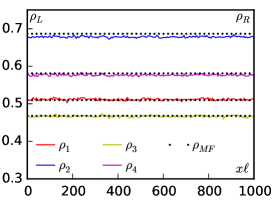
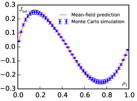
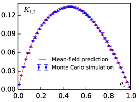
Figure 19: Simulation results for $N=10$ TASEPs on a ring. Even lanes ($i=2,4,6,8,10$) correspond to right-going TASEPs whereas odd lanes ($i=1,3,5,7,9$) correspond to left-going TASEPs; in all cases, the hopping rate is $p_{i}=1$. The transverse rates are: $d_{1,2}=0.95$, $d_{2,3}=0.55$, $d_{3,4}=0.72$, $d_{4,5}=0.62$, $d_{5,6}=0.79$, $d_{6,7}=0.99$, $d_{7,8}=0.81$, $d_{8,9}=0.61$, $d_{9,10}=0.93$, $d_{10,1}=0.53$, $d_{2,1}=0.05$, $d_{3,2}=0.45$, $d_{4,3}=0.02$, $d_{5,4}=0.32$, $d_{6,5}=0.19$, $d_{7,6}=0.49$, $d_{8,7}=0.01$, $d_{9,8}=0.41$, $d_{10,9}=0.03$, $d_{1,10}=0.23$. Left: profiles of densities of lanes 1 to 4 are shown for $\rho_{1}^{L}=\rho_{1}^{R}=0.51$. Center: total longitudinal current as a function of $\rho_{1}$: the maximum is at $\rho_{1}^{M}=0.15$ while the minimum is at $\rho_{1}^{m}=0.75$ (Monte Carlo values). Right: transverse current between lane 1 and 2 (currents between all other pairs of lanes are the same).

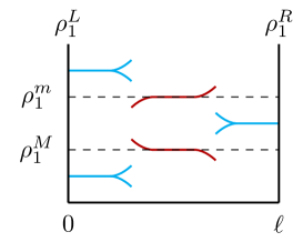
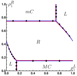
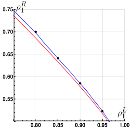
Figure 20: Simulation results for $N=10$ TASEPs on a ring, with the same parameters as in Fig 19. Left: possible connections of equilibrated plateaux predicted by the linear stability analysis. Center: phase diagram where now red lines represent the result of the extremal current principle applied to the mean-field prediction and blue lines represent the result of the extremal current principle applied to the Monte Carlo simulation of $J_{\rm tot}$. Black dots represent numerical simulations (with quite invisible errorbars) in the vicinity of phase transition lines. The possible phases are Left Phase, Right Phase, Maximal Current Phase and minimal Current Phase. Right: zoom on a region where the discrepancy between mean-field prediction and Monte Carlo simulation results are appreciable.

6 Conclusions

In this article we have shown that a generalized extremal current principle can be used to construct the phase diagram of multilane driven diffusive systems under the hypothesis that the hopping rate along one lane does not depend on the occupancies of the neighbouring lanes, and that the hopping rate between lanes increases with the occupancy of the departing site and decreases with the occupancy of the target site. This allowed us to show that the phase diagrams of such systems are equivalent to those of single-lane systems, though with much more complicated current-density relations. It validates the frequently made hypothesis that molecular motors hopping along microtubules can be effectively describe by single lane models. In all our modelling, we have used equilibrated reservoirs; all our results extends to the case of non-equilibrated reservoirs but with two new boundary layers connecting the bulk equilibrated plateaux with the reservoirs, as shown in Fig 7. In this case, the relation between the densities of the bulk plateaux and those of the reservoirs are, however, not known in general.

Our theory is based on the analysis of hydrodynamic descriptions of lattice gases. To apply our approach to precise microscopic models one thus needs to construct such continuous descriptions, for instance using mean-field approximations such as the simple mean-field approximation we have employed here. Those are known to fail when correlations between neighbouring sites are important but we have shown that the generalized extremal current principle still holds with respect to the exact current-density relation which can be measured in a simulation.

The existence of transverse currents, impossible for single and two lane systems, nevertheless leads to interesting phenomenology. For instance, we have shown that when a system has different transverse flows imposed at its boundaries, driven-diffusive systems can have a bulk behaviour strongly different from diffusive systems. For the latter, the transverse flow smoothly interpolates between its imposed bundary conditions whereas driven-dffusive systems can exhibit ‘shear-localization’. The system then splits into homogeneous parts with constant transverse flows separated by sharp interface(s).

Our study extends the physics of one-dimensional boundary driven phase transitions to more complex systems and in particular to 2D lattices. It would be interesting to further pursue this approach with more general lattice structures, such as the network of filaments encountered in active gels [34].

Appendix A Dynamical stability of equilibrated plateaux

Consider a small perturbation $\delta\rho$ around the equilibrated plateau solution (see Section 3.1) which may be decomposed as

$$\rho_{i}(x,t)=\rho_{i}^{0}+\sum_{q}\delta\rho_{i}^{q}(t)\exp(iqx)\;,$$ (40)

where $q=2\pi n$ with $n=1,\ldots,\ell-1$. We will denote by $|\delta\rho^{q})$ the vector $(\delta\rho_{1}^{q},\ldots\delta\rho_{N}^{q})$. Inserting expression (40) into the mean-field equations (2) and expanding to first order in $\delta\rho_{i}^{q}$ yields the equation

$$\frac{\text{d}}{\text{d}t}|\delta\rho^{q})=C^{q}\cdot|\delta\rho^{q}),$$ (41)

where the matrix $C^{q}$ is defined by

$$C_{ii}^{q}=-D_{i}q^{2}-\text{i}-{\rm i}qJ_{i}^{i}+\sum_{j\neq i}K_{ji}^{i}\;;\qquad C^{q}_{ij\neq i}=K_{ji}^{j},$$ (42)

with $J_{i}^{i}\equiv\partial_{\rho_{i}}J_{i}(\rho^{0})$. Note that the matrix $C_{ii}^{q}$ can be defined for any positive real number $q$ and not only for the discrete values $q=2\pi n$. As we now show, the eigenvalues $\lambda_{i}(q)$ of the matrix $C^{q}$ always have negative real parts and $|\delta\rho^{q}(t))$ thus vanishes at large time.

For $q=0$, $C^{q}$ is a Markov matrix and none of its eigenvalues $\lambda_{i}(0)$ has a positive real part: Eq. (42) indeed shows the sum of each column elements to vanish for $q=0$. Conversely, when $q\rightarrow\infty$, $\lambda_{i}(q)\sim-D_{i}q^{2}$ and $\lambda_{i}(q)$ thus has a negative real part. Physically, the short wave-length perturbations are stabilized by the diffusive terms while the large wave-length perturbations are stabilized by the exchange between lanes.

The eigenvalues of a matrix are continuous functions in $\mathbb{C}$ of its coefficients. For $C(q)$ to have an eigenvalue with a positive real part, we need $q^{*}\in[0,\infty[$ such that at least one eigenvalue satisfies ${\rm Re}(\lambda_{i}(q^{*}))=0$, which means

$$\exists|v)\neq 0\qquad\text{such that}\qquad C^{q}|v)=i\varphi|v),\quad\text{where}\quad\varphi\in\mathbb{R}.$$ (43)

The matrix $A\equiv C^{q}-i\varphi\mathbb{I}$ is thus singular. It is however easy to see that $A^{t}$, the transpose of $A$, is a strictly diagonally dominant matrix, i.e.

$$|A^{t}_{ii}| = |D_{i}q^{2}+\Big{(}\sum_{j\neq i}K_{ij}^{i}\Big{)}+\text{i}(qJ_{i}^{i}+\varphi)|$$

$$> \sum_{j\neq i}|A^{t}_{ij}|=\sum_{j\neq i}|K_{ij}^{i}|=|\sum_{j\neq i}K_{ij}^{i}|\;.$$

The Gershgorin circle theorem states that all eigenvalues of a square matrix $B$ can be found within one of the circles centered on $B_{ii}$ of radii $\sum_{j\neq i}|B_{ij}|$. This implies that strictly diagonally dominant matrices cannot be singular: $A^{t}$ and $A$ are thus invertible. Therefore, the matrix $C(q)$ cannot have purely imaginary eigenvalues: all its eigenvalues thus have a negative real part for all $q$. Equilibrated plateaux are thus always dynamically stable when $J_{i}$ is only a function of $\rho_{i}$ and when equations (3) are satisfied. This can break down for more general systems, when interactions between the lanes are allowed for [32].

Appendix B Connecting bulk plateaux to equilibrated reservoirs using the eigenvectors of $M$

This appendix is divided in two parts. In the first part, we show that the spectrum of $M$ is composed of either $(i)$ $N$ eigenvalues with positive real parts and $N-1$ eigenvalues with negative real parts, or $(ii)$ $N-1$ eigenvalues with positive real parts and $N$ eigenvalues with negative real parts.

The second part then shows that these two cases respectively correspond to plateaux which can only be observed in Left and Right phases.

B.1

We begin by considering a semi-infinite problem with a reservoir at the left end of the system. Let us assume that the equilibrated plateaux densities $\rho^{\,\rm p}_{j}$ are determined by single-valued (a priori unknown) functions of the reservoir densities $|\rho^{\,L})$:

$$\forall j\qquad\rho_{j}^{\,\rm p}=H_{j}(\rho_{1}^{\,L},\dots,\rho_{N}^{\,L}),$$ (44)

When the reservoir is equilibrated, one simply has $\rho_{j}^{\,\rm p}=H_{j}(\rho_{j}^{\,L})=\rho^{\,L}_{j}$. We now focus on perturbations of equilibrated reservoirs and show that the space of perturbations $|\delta\rho^{\,L})$ that leave $|\rho^{\,\rm p})$ invariant is of dimension $N-1$.

To see this, let us look at the consequence of an infinitesimal perturbation $|\delta\rho^{\,L})$ of the reservoir densities. This perturbation results in a change of bulk equilibrated densities from $|\rho^{\,\rm p})$ to $|\rho^{\,\rm p})+|\delta\rho^{\,\rm p})$, with

$$\delta\rho^{\,\rm p}_{j}=\sum_{i}\left(\partial_{\rho_{i}^{\,L}}H_{j}\right)\delta\rho_{i}^{\,L}\;.$$ (45)

which can be rewritten in matrix form as

$$|\delta\rho^{\,\rm p})=H^{\prime}|\delta\rho^{\,L})\quad\text{where}\quad H^{\prime}_{ji}\equiv\partial_{\rho_{i}^{\,L}}H_{j}.$$ (46)

By definition the bulk densities $|\rho^{\,\rm p})+|\delta\rho^{\,\rm p})$ are still equilibrated. Therefore, as shown in section 4.1, $|\delta\rho^{\,\rm p})=\epsilon|\delta\rho^{\,\rm 0})$, where $\epsilon$ is a small parameter and thus

$$H^{\prime}|\delta\rho^{\,L})=\epsilon|\rho^{\,\rm 0})$$ (47)

The key observation is that since equation (47) holds for any perturbation $|\delta\rho^{\,L})$, the matrix $H^{\prime}$ projects any vector $|\delta\rho^{\,L})$ onto the direction $|\delta\rho^{\,\rm 0})$. Furthermore, we now show that $H^{\prime}$ is indeed a projector satisfying $(H^{\prime})^{2}=H^{\prime}$. Since $H^{\prime}|\delta\rho^{\,L})\propto|\delta\rho^{0})$, the image of $H^{\prime}$ is $\text{Span}|\delta\rho^{0})$. If we consider an equilibrated boundary density vector $|\rho^{\,L})$ then $|\rho^{\,L}+\epsilon\delta\rho^{0})$ is also equilibrated, which implies $H(|\rho^{\,L}+\epsilon\delta\rho^{0}))=|\rho^{\,L})+\epsilon|\delta\rho^{0})$. Then by linearisation, $H^{\prime}|\delta\rho^{0})=|\delta\rho^{0})$. Since (47) holds for all $|\delta\rho^{\,L})$, $H^{\prime}$ thus satisfies $(H^{\prime})^{2}=H^{\prime}$.

We may now invoke a basic theorem of linear algebra that for a projector, here $H^{\prime}$, the direct sum of the image space and the kernel gives the full $N$ dimensional vector space :

$$\mathbb{R}^{N}=\text{Span}(|\delta\rho^{0}))\oplus\ker(H^{\prime})\;.$$ (48)

Note that $\ker(H^{\prime})$ is the space of perturbations $|\delta\rho^{\,L})$ that leave $|\rho^{\,\rm p})$ invariant (since $H^{\prime}|\delta\rho^{\,\rm r})=|\delta\rho^{\,\rm p})=0$). Therefore the space of perturbations $|\delta\rho^{\,L})$ that leave the bulk density vector invariant is of dimension $N-1$.

To connect these perturbations to the eigenvectors of the matrix $M$, let us consider a given equilibrated plateau $|\rho^{\,\rm p})$ and ask which reservoir density vectors $|\rho^{\,\rm p}+\delta\rho^{\,\rm r})$ it can be connected to through a perturbation $|\delta\rho(x))$. Such a perturbation can be decomposed using the eigenvectors of $M$ as in equation (15):

$$|\delta\rho(x))=\sum_{k=1}^{2N-1}\alpha_{k}|\delta\rho^{k})e^{\lambda_{k}x}\;.$$ (49)

By definition, $|\delta\rho(x))$ vanishes in the bulk of the system (see Fig. 8) so there is no $\alpha_{0}$ term in the sum.

The sum in (49) is restricted to ${\rm Re}(\lambda_{k})<0$ when connecting to left reservoirs as terms coming from eigenvectors with eigenvalues with ${\rm Re}(\lambda_{k})\geq 0$ would not die out in the bulk. Since $|\delta\rho(x=0))=|\delta\rho^{\,\rm r})$ , the perturbations (49) need to span the sets of left reservoir perturbations that leave $|\rho^{\,\rm p})$ invariant. Since the vector spaces of such perturbations are $N-1$ dimensional, one needs at least $N-1$ eigenvectors with ${\rm Re}(\lambda_{k})<0$.

Conversely, the same reasoning for a semi-infinite system connected to a reservoir on its right would lead to the conclusion that one needs at least $N-1$ eigenvectors with ${\rm Re}(\lambda_{k})>0$.

To conclude the first part of this appendix, let us summarize what we know on the spectrum of the matrix $M$. Since it has $2N$ eigenvectors, one of which is associated with the eigenvalue $\lambda_{0}=0$, among the remaining $2N-1$ there must be either $N-1$ eigenvectors with ${\rm Re}(\lambda_{k})<0$ and $N$ eigenvectors with ${\rm Re}(\lambda_{k})>0$ or $N-1$ eigenvectors with ${\rm Re}(\lambda_{k})>0$ and $N$ eigenvectors with ${\rm Re}(\lambda_{k})<0$.

B.2

We now show that the first case, with $N-1$ eigenvectors with ${\rm Re}(\lambda_{k})<0$ and $N$ eigenvectors with ${\rm Re}(\lambda_{k})>0$, corresponds to a Left Phase.

1. Connection to left reservoirs. As we have shown, there is a space of perturbations $|\delta\rho^{\,\rm r})$ of dimension $N-1$ that leave $|\rho^{\,\rm p})$ invariant. Since these are spanned by the $N-1$ eigenvectors with ${\rm Re}(\lambda_{k})<0$, the latter constitute a basis of $\ker[H^{\prime}(\rho^{\,\rm p})]$ and one can construct a perturbation $|\delta\rho(x))$ that connects $\rho^{\,\rm p}$ to the reservoir $\rho^{\,\rm p}+\delta\rho^{\,\rm r}$.

   Let us now consider a small equilibrated perturbation $|\delta\rho^{\,\rm r})=\alpha|\delta\rho^{0})$ of $|\rho^{\,\rm r})$ for which there exists a stationary profile connecting $|\rho^{\,\rm p})$ to $|\rho^{\,\rm r})+\alpha|\delta\rho^{0})$. Since the profile connects to the reservoir at $x=0$, one needs to find a decomposition of $|\delta\rho(x))$ such that

   $$|\delta\rho(0))=\sum_{{\rm Re}(\lambda_{k})<0}\alpha_{k}|\delta\rho^{k})=\alpha|\delta\rho^{0}).$$ (50)

   However, since $H^{\prime}$ is a projection on $|\delta\rho^{0})$ and $\text{Span}(|\delta\rho^{k}),{\rm Re}(\lambda_{k})<0)=\ker(H^{\prime})$, Eq. (48) applies and the intersection between $\ker H^{\prime}$ and $\text{Span}[|\delta\rho^{0})]$ is the empty set. As a consequence, $\delta\rho_{i}(0)$, which belongs to both sets because of (50), is the null vector ($\alpha_{k}=\alpha=0$): the sole equilibrated reservoir to which $\rho^{\,\rm p}$ can be connected to the left corresponds to $|\rho^{\,\rm r})=|\rho^{\,\rm p})$.

2. Connection to right reservoirs. We now consider only the $N$ eigenvectors with ${\rm Re}(\lambda_{k})>0$. While they still span $\ker(H^{\prime})$, and $|\rho^{\,\rm p})$ can still be connected to unequilibrated reservoirs on the right, the $|\delta\rho^{k})$ need not anymore be in $\ker(H^{\prime})$. Let us show that $|\rho^{\,\rm p})$ can be connected to an equilibrated reservoir on the right with $|\delta\rho^{\,\rm r})\neq 0$. Again, this requires a perturbation $|\delta\rho)$ which satisfies

   $$\sum_{{\rm Re}(\lambda_{k})>0}\alpha^{k}|\delta\rho^{k})=\epsilon|\delta\rho^{0}),$$ (51)

   Let us first remember that the eigenvectors $|v^{k}\rangle$ of $M(\rho^{\,\rm p})$ are $2N$-dimensional and that $|\delta\rho^{k})$ are simply the second half of the components of these vectors. We want to show that $|\delta\rho^{0})\in\text{Span}[|\delta\rho^{k}),{\rm Re}(\lambda_{k})>0]$. To do so, we consider the vector space $X=\{(x_{1},\dots,x_{N},0,\dots,0),x_{i}\in\mathbb{R}\}$ of dimension $N$. The eigenvector associated to $\lambda=0$ is $|v^{0}\rangle=(0,\dots,0,\delta\rho^{0}_{1},\dots,\delta\rho^{0}_{N})$ and clearly $|v^{0}\rangle\notin X$. From this we can say that

   $$\text{dim}(X+\text{Span}|v^{0}\rangle)=N+1.$$

   Since one also has $\text{dim}[\text{Span}[|v^{k}\rangle,{\rm Re}(\lambda_{k})>0]]=N$ and $\text{dim}[(X+\text{Span}|v^{0}\rangle)+(\text{Span}|v^{k}\rangle)]\leq 2N$ (the total space is $2N$ dimensional), it follows that

   $$\text{dim}[(X+\text{Span}|v^{0}\rangle)+(\text{Span}|v^{k}\rangle)] < \text{dim}(X+\text{Span}|v^{0}\rangle)+$$

   $$+\text{dim}(\text{Span}|v^{k}\rangle)=2N+1\;.$$

   The intersection between the two spaces is not the empty set

   $$(X+\text{Span}|v^{0}\rangle)\cap(\text{Span}|v^{k}\rangle)\neq\emptyset$$ (52)

   and there exists a vector $|w\rangle\in X+\text{Span}|v^{0}\rangle$ of the form $|w\rangle=(x_{1},\dots,x_{N},\epsilon\delta\rho^{0}_{1},\dots,\epsilon\delta\rho^{0}_{N})$ which is also in $\text{Span}|v^{k}\rangle$. This vector can be written as $|w\rangle=\sum_{{\rm Re}(\lambda_{k})>0}\alpha^{k}|v^{k}\rangle$ and the equality of the second half of the components yield

   $$\forall i\quad\sum_{{\rm Re}(\lambda_{k})>0}\alpha^{k}\delta\rho_{i}^{k}=\epsilon\delta\rho_{i}^{0}\;.$$ (53)

   One can thus construct a perturbation, spanned by the $|v_{k}\rangle$ with ${\rm Re}(\lambda_{k})>0$, which is proportional to $|v_{k}^{0}\rangle$ and connects $|\rho^{\,\rm p})$ to an equilibrated reservoir $|\rho^{\,\rm p})+\epsilon|\delta\rho^{0})$ with $\epsilon\neq 0$.

Conversely, the same reasoning would show that, for equilibrated reservoirs, a plateau with $N$ eigenvalues with ${\rm Re}(\lambda_{k})<0$ can only be observed in a Right Phase.

Appendix C Transverse current in parallel TASEPs

We will now show that a definition of the transverse current such as the one given in (33) cannot possibly yield a change of sign in $K$, i.e., $K=0\Leftrightarrow\rho_{i}=\rho_{i\pm 1}=0,1$. To show this, consider at first $N=3$ and let us take $K=0$. Then we have

$$d_{12}\rho_{1}(1-\rho_{2}) = d_{21}\rho_{2}(1-\rho_{1})$$

$$d_{23}\rho_{2}(1-\rho_{3}) = d_{32}\rho_{3}(1-\rho_{2})$$

$$d_{31}\rho_{3}(1-\rho_{1}) = d_{13}\rho_{1}(1-\rho_{3}).$$ (54)

Solving the system of equation for $\rho_{i}$ ($i=1,2,3$) yields the equality $(d_{12}d_{23}d_{31}-d_{21}d_{32}d_{13})(1-\rho_{i})\rho_{i}=0$, from which we can easily see that either $\rho_{i}=0$ or $\rho_{i}=1$, i.e. the two solutions that we excluded, or $d_{12}d_{23}d_{31}=d_{21}d_{32}d_{13}$. This last condition corresponds to an exactly null transverse current for any value of the density.

This result can be generalized to the case of an $N-$lane system by using the recursion relation

$$\rho_{i+1}=\frac{\prod_{j=1}^{i}d_{j,j+1}\rho_{1}}{\prod_{j=1}^{i}d_{j,j+1}\rho_{1}+\prod_{j=1}^{i}d_{j+1,j}(1-\rho_{1})}$$ (55)

and by imposing the periodic condition at the boundary: $\rho_{N+1}=\rho_{1}$. Then we find that in order to have $K=0$ for some $\rho_{i}\neq 0,1$ one must have $\prod_{j=1}^{N}d_{j,j+1}=\prod_{j=1}^{N}d_{j+1,j}$, which however implies $K=0\ \forall\ \rho_{i}\neq 0,1$. We have shown here only the necessary condition, but the sufficent one can be proved by taking (33) and setting $\prod_{j=1}^{N}d_{j,j+1}=\prod_{j=1}^{N}d_{j+1,j}$ for generic $N$.

Note that this appendix shows that $K$ cannot vanish if $\rho_{i}\neq 0,1$ unless it is always zero. One could imagine, however, that $K$ changes sign discontinuously, without ever satisfying $K=0$. This never occurs with the simple choice of rates $K_{ij}$ we have considered (which is not very surprising since $K$ can be shown to be the solution of a polynomial equation whose coefficients are continuous functions of $\rho_{1}$). More complicated transverse hopping rates, not considered in this article, leading to multiple possibilities of equilibrated plateaux for a given value of $\rho_{1}$, could, however, exhibit more complicated behaviour.

References

- [1] B. Schmittmann and R. K. P. Zia 1995 Statistical mechanics of driven diffusive systems, volume 17 of Phase transitions and critical phenomena Academic Press, New York
- [2] D. Mukamel 2000 Phase transitions in nonequilibrium systems in Soft and Fragile Matter: Nonequilibrium Dynamics, Metastability and Flow IoP publishing, Bristol
- [3] J. Krug 1991 Boundary-induced phase transitions in driven diffusive systems, Phys. Rev. Lett. 67
- [4] B Derrida, E Domany and D Mukamel 1992 An exact solution of a one-dimensional asymmetric exclusion model with open boundaries, J. Stat. Phys 69 667
- [5] B Derrida, M. R. Evans, V. Hakim, V. Pasquier 1993 Exact solution of a 1D asymmetric exclusion model using a matrix formulation J. Phys. A Math. Gen. 26 1493
- [6] G. Schutz and E. Domany 1993 Phase transitions in an exactly soluble one-dimensional exclusion process J. Stat. Phys. 72 277
- [7] V. Popkov, and G. M. Schutz 1999 Steady-state selection in driven diffusive systems with open boundaries, EPL 48, 257
- [8] J. S. Hager, J. Krug, V. Popkov, and G. M. Schutz 2001 Minimal current phase and universal boundary layers in driven diffusive systems, Phys. Rev. E 63, 056110
- [9] C. T. MacDonald, J. H. Gibbs, A. C. Pipkin 1968 Kinetics of biopolymerization on nucleic acid templates, Biopolymers 6(1): 1-25
- [10] Y. Aghababaie, G. I. Menon, and M. Plischke 1999 Universal properties of interacting brownian motors Phys. Rev. E, 59 2578
- [11] S. Klumpp and R. Lipowsky 2003 Traffic of molecular motors through tube-like compartments J. Stat. Phys. 113 233
- [12] K.E.P. Sugden, M. R. Evans, W.C.K Poon, N. D. Read 2007 Model of hyphal tip growth involving microtubule-based transport Phys. Rev. E 75 031909
- [13] J. Tailleur, M.R. Evans, Y. Kafri 2009 Non-equilibrium phase transitions in tubulation by molecular motors Phys. Rev. Lett. 102, 118109
- [14] A. Schadschneider 2008 Modelling of transport and traffic problems Lecture Notes In Computer Science 5191: 22-31, (2008)
- [15] T. Chou, K Mallick and R K P Zia 2011 Non-equilibrium statistical mechanics: from a paradigmatic model to biological transport Rep. Prog. Phys. 74 116601
- [16] P. Greulich, L. Ciandrini, R. J. Allen, M. C. Romano 2012 A mixed population of competing TASEPs with a shared reservoir of particles Phys. Rev. E 85 011142
- [17] K. Nishinari, Y. Okada, A. Schadschneider, D. Chowdhury 2005 Intracellular transport of single-headed molecular motors KIF1A Physical Review Letters 95 118101
- [18] H. Hilhorst, C. Appert-Rolland 2012 A multi-lane TASEP model for crossing pedestrian traffic flows, J. Stat. Mech. P06009
- [19] V. Popkov and G. M. Schutz 2003 Shocks and excitation dynamics in a driven diffusive two-channel system J. Stat. Phys. 112, 523
- [20] V Popkov and M Salerno 2004 Hydrodynamic limit of multichain driven diffusive models 2004 Phys. Rev. E 69 046103
- [21] E Pronina and A.B. Kolomeisky 2004 Two-channel totally asymmetric simple exclusion processes J. Phys. A Math. Gen. 37 9907-9918
- [22] R. J. Harris and R. B. Stinchcombe 2005 Ideal and disordered two-lane traffic models Physica A 354 582-596
- [23] B. Schmittmann, J. Krometis, and R. K. P. Zia, 2005 Will jams get worse when slow cars move over? Europhys. Lett. 70, 299-305
- [24] R. Juhasz 2007 Weakly coupled, antiparallel, totally asymmetric simple exclusion processes Phys. Rev. E 76 021117
- [25] T. Reichenbach, T. Franosch and E. Frey 2007 Traffic jams induced by rare switching events in two-lane transport New J. Phys. 9, 159
- [26] R. Jiang, M-B Hu, Y-H Wu and Q-S Wu 2008 Weak and strong coupling in a two-lane asymmetric exclusion process Phys. Rev. E 77, 041128
- [27] D Chowdhury, A Garai and J-S Wang 2008 Traffic of single-headed motor proteins KIF1A: Effects of lane changing Phys. Rev. E 77 050902
- [28] R. Jiang, K Nishinari, M-B Hu, Y-H Wu and Q-S Wu, 2009 Phase separation in a bidirectional two-lane asymmetric exclusion process J. Stat. Phys 136,73
- [29] C. Schiffmann, C Appert-Rolland and L. Santen 2010 Shock dynamics of two-lane driven lattice gases J. Stat. Mech: Theor. Exp. P06002
- [30] V. Yadav, R. Singh and S. Mukherji 2012 Phase-plane analysis of driven multi-lane exclusion models, Journal of Statistical Mechanics: Theory and Experiment, P04004
- [31] Y.-Q. Wang, R. Jiang, Q.-S. Wu and H.-Y. Wu 2014 Phase transitions in three-lane TASEPs with weak coupling Modern Physics Letters B 28, 1450123
- [32] M. R. Evans, Y. Kafri, K. E. P. Sugden, J. Tailleur 2011 ‘Phase diagram of two-lane driven diffusive systems J. Stat. Mech., P06009
- [33] M Basu and P K Mohanty 2010 Asymmetric simple exclusion process on a cayley tree Journal of Statistical Mechanics: Theory and Experiment P10014
- [34] I Neri, N Kern, and A. Parmeggiani 2011 Totally asymmetric simple exclusion process on networks Physical Review Letters 107, 068702
- [35] P. Mottishaw, B. Waclaw and M. R. Evans 2013 An exclusion process on a tree with constant aggregate hopping rate Journal of Physics A: Mathematical and Theoretical 405003 46
- [36] T. Chou, K. Mallick and R. K. P. Zia 2011 Non-equilibrium statistical mechanics: Fundamental issues, a paradigmatic model, and applications to biological transport, Reports on Progess in Physics 74, 116601
- [37] S. Mukherji 2009 Fixed points and boundary layers in asymmetric simple exclusion processes Phys. Rev. E 79 041140
- [38] B Saha and S Mukherji 2013 Coupling driven exclusion and diffusion processes on parallel lanes: boundary induced phase transitions and boundary layers Journal of Statistical Mechanics: Theory and Experiment, P09004
- [39] A. K. Gupta, I. Dhiman 2014 Asymmetric coupling in two-lane simple exclusion processes with Langmuir kinetics: Phase diagrams and boundary layers, Physical Review E, 89, 022131
- [40] J. Tailleur, J. Kurchan, V. Lecomte 2008 Mapping out of equilibrium into equilibrium in one-dimensional transport models Journal of Physics A: Math. Theor 41, 50500
- [41] T. Tripathi and D. Chowdhury 2008 Interacting RNA polymerase motors on a DNA track: effects of traffic congestion and intrinsic noise on RNA synthesis Phys Rev E 77, 011921
- [42] R. A. Blythe, M. R. Evans 2007 Nonequilibrium steady states of matrix product form: a solver’s guide, J. Phys. A Math. Theor. 40: R333-R441
- [43] M. Ebbinghaus, C. Appert-Rolland, and L. Santen 2010 Bidirectional transport on a dynamic lattice Phys. Rev. E 82, 040901
- [44] R.D. Vale, Y.Y. Toyoshima 1988 Rotation and translocation of microtubules in vitro induced by dyneins from Tetrahymena cilia Cell 52, 459
- [45] V. Bormuth, B. Nitzsche, F. Ruhnow, et al, 2012 The Highly Processive Kinesin-8, Kip3, Switches Microtubule Protofilaments with a Bias toward the Left. Biophys. J. 103 L4
- [46] D. Oriola, S. Roth, M. Dogterom, J. Casademunt 2015 Formation of Helical Membrane Tubes around Microtubules by Single-Headed Kinesin KIF1A Nat Commun 6, 8025
- [47] C. Leduc, K. Padberg-Gehle, V. Varga, D. Helbing, S. Diez, J. Howard 2012 Molecular crowding creates traffic jams of kinesin motors on microtubules Proc. Natl. Acad. Sci. USA 109, 6100
- [48] R. G. Larson 1999 The structure and rheology of complex fluids, Oxford University Press (New York)
- [49] A. P. Solon, Y. Fily, A. Baskaran, M. E. Cates, Y. Kafri, M. Kardar, J. Tailleur 2015 Pressure is not a state function for generic active fluids Nat. Phys. 11, 673-678