A comparison of macroscopic models describing the collective response of sedimenting rod-like particles in shear flows.

Abstract

We consider a kinetic model, which describes the sedimentation of rod-like particles in dilute suspensions under the influence of gravity. This model has recently been derived by Helzel and Tzavaras in [6]. Here we restrict our considerations to shear flow and consider a simplified situation, where the particle orientation is restricted to the plane spanned by the direction of shear and the direction of gravity. For this simplified kinetic model we carry out a linear stability analysis and we derive two different macroscopic models which describe the formation of clusters of higher particle density. One of these macroscopic models is based on a diffusive scaling, the other one is based on a so-called quasi-dynamic approximation. Numerical computations, which compare the predictions of the macroscopic models with the kinetic model, complete our presentation.

Key words: rod-like particles, sedimentation, linear stability, moment closure, quasi-dynamic approximation, diffusive scaling

1 Introduction

We discuss different mathematical models which describe the sedimentation process for dilute suspensions of rod-like particles under the influence of gravity. The sedimentation of rod-like particles has been studied by several authors in theoretical as well as experimental and numerical works, see Guazzelli and Hinch [5] for a recent review paper. Experimental studies of Guazzelli and coworkers [7, 8, 10] start with a well stirred suspension. Under the influence of gravity, a well stirred initial configuration is unstable and it is observed that clusters with higher particles concentration form. These clusters have a mesoscopic equilibrium width. Within a cluster, individual particles tend to align in the direction of gravity.

The basic mechanism of instability and cluster formation was described in a fundamental paper of Koch and Shaqfeh [9]. In Helzel and Tzavaras [6], we recently derived a kinetic model which describes the sedimentation process for dilute suspensions of rod-like particles. By applying moment closure hypotheses and other approximations to an associated moment system, we derived macroscopic models for the evolution of the rod density and compared the prediction of such macroscopic models to the original kinetic model using numerical experiments. This is done in [6] for rectilinear flows with the particles taking values on the sphere. Here, to simplify and explain our considerations we restrict to the simpler case of shear flows and for particles with orientations restricted to take values on the plane. While the derivations in [6] are often quite technical, the restriction to the simpler situation provides a useful and technically simple setting in order to understand the underlying ideas. In addition, as explained in the present work, the form of the derived macroscopic equations is identical in both cases apart from the values of numerical constants that capture the effect of dimensionality in the microstructure. Therefore, we hope that this paper will make our results accessible and useful for a wider community interested in the modelling of complex fluids.

The rest of the paper is organised as follows. In Section 2 we present the kinetic model from [6] and a simplification, which is obtained for shear flows. We then present the simplified model system, obtained by restricting the orientation of particles to move in a plane. In Section 3 we derive a nonlinear moment closure system which forms the basis for all further considerations. In Section 4, a linearization of the moment closure system is used to study the linear instability of shear flows. We show that a nonzero Reynolds number provides a wavelength selection mechanism. An asymptotic analysis of the largest eigenvalue around $Re=0$ explains this behavior. In Section 5, we depart from a closure of the non-linear moment system and use a quasi-dynamic approximation in order to derive an effective equation for the evolution of the macroscopic density. The basic assumption behind this approximation is that the behavior of the second order moments can be replaced by equilibrium relations in the moment closure system. In Section 6, we present a different set of macroscopic equations for the density obtained via the so-called diffusive limit. We observe that the diffusive approximation leads to a typical Keller-Segel model, while the quasi-dynamic approximation leads to a flux-limited Keller-Segel type model. In Section 7 we present numerical results comparing the diffusive approximation and the quasi-dynamic approximation to the full kinetic model. Although the idea of diffusive scalings to obtain macroscopic equations is commonplace in kinetic theory, it has not been applied (to our knowledge) in the sedimentation problem. For reasons of comparison, we present in an appendix, a derivation of the hyperbolic and diffusive scaling equations for general rectilinear flows where the direction of the rod-like particles takes values on the sphere.

2 A kinetic model for the sedimentation of rod-like particles

We consider a kinetic model for the sedimentation of rod-like particles, derived in Helzel and Tzavaras [6], based on kinetic models for dilute suspensions of rod-like particles that are described in Doi and Edwards [4].

In non-dimensional form, the kinetic model reads

$$\begin{split}\partial_{t}f+\nabla_{\boldsymbol{x}}\cdot\left(\boldsymbol{u}f\right)&+\nabla_{\boldsymbol{n}}\cdot\left(P_{\boldsymbol{n}^{\bot}}\nabla_{\boldsymbol{x}}\boldsymbol{u}\boldsymbol{n}f\right)-\nabla_{\boldsymbol{x}}\cdot\left(D(\boldsymbol{n})\boldsymbol{e}_{3}f\right)\\ &=D_{r}\Delta_{\boldsymbol{n}}f+\gamma\nabla_{\boldsymbol{x}}\cdot\left(D(\boldsymbol{n})\nabla_{\boldsymbol{x}}f\right)\\ \sigma&=\int_{S^{d-1}}\left(d\boldsymbol{n}\otimes\boldsymbol{n}-I\right)f\,d\boldsymbol{n}\\ Re\left(\partial_{t}\boldsymbol{u}+\left(\boldsymbol{u}\cdot\nabla_{\boldsymbol{x}}\right)\boldsymbol{u}\right)&=\Delta_{\boldsymbol{x}}\boldsymbol{u}-\nabla_{\boldsymbol{x}}p+\delta\gamma\nabla_{\boldsymbol{x}}\cdot\sigma+\delta\left(\bar{\rho}-\int_{S^{d-1}}f\,d\boldsymbol{n}\right)\boldsymbol{e}_{3}\\ \nabla_{\boldsymbol{x}}\cdot\boldsymbol{u}&=0.\end{split}$$ (1)

Here $f=f(t,\boldsymbol{x},\boldsymbol{n})$ is a distribution function of particles at time $t$, space $\boldsymbol{x}\in\mathbb{R}^{d}$ and orientation $\boldsymbol{n}\in S^{d-1}$, $\boldsymbol{u}=\boldsymbol{u}(t,\boldsymbol{x})$ is the velocity of the solvent, $p=p(t,\boldsymbol{x})$ is the pressure and $\sigma=\sigma(t,\boldsymbol{x})$ is the polymeric stress acting on the fluid. Gradient, divergence and Laplacian on the sphere are denoted by $\nabla_{\boldsymbol{n}}$, $\nabla_{\boldsymbol{n}}\cdot$ and $\Delta_{\boldsymbol{n}}$, while gradient and divergence in the macroscopic space are denoted by $\nabla_{\boldsymbol{x}}$ and $\nabla_{\boldsymbol{x}}\cdot$. The term

$$P_{\boldsymbol{n}^{\bot}}\nabla_{\boldsymbol{x}}\boldsymbol{u}\boldsymbol{n}=\nabla_{\boldsymbol{x}}\boldsymbol{u}\boldsymbol{n}-\left(\nabla_{\boldsymbol{x}}\boldsymbol{u}\boldsymbol{n}\cdot\boldsymbol{n}\right)\boldsymbol{n}$$

is the projection of the vector $\nabla_{\boldsymbol{x}}\boldsymbol{u}\boldsymbol{n}$ onto the tangent space at $\boldsymbol{n}$ while $D(\boldsymbol{n})=I+\boldsymbol{n}\otimes\boldsymbol{n}$. Finally, the unit vector $-\boldsymbol{e}_{3}$ points into the direction of gravity. We note that $D_{r}$, $\delta$, $\gamma$ and $Re$ are non-dimensional numbers and refer to [6] for their description. Furthermore, the constant $\bar{\rho}$ describes the average density of the suspended rods; it can be easily absorbed into the pressure, by modifying it to account for the hydrostatic pressure, but we prefer to put it as a factor that equilibrates the body force.

The second and the fourth term on the left hand side of (1)₁ model transport of the center of mass of the particles due to the macroscopic flow velocity and due to gravity, respectively. The third term on the left hand side models the effect of rotation of the axis of the microstructure due to a macroscopic velocity gradient. The terms on the right hand side of the first equation in (1) describe rotational and translational diffusion respectively. Equation (1)₂ defines the stress tensor emerging from the microstructure while (1)₃ and (1)₄ describe the macroscopic flow of the solvent.

In this paper we mainly restrict our considerations to the study of shear flows, i.e. we consider the case $\boldsymbol{u}=(0,0,w(t,x))^{T}$. The director $\boldsymbol{n}$ may in general take values in $S^{2}$, which means that the rod-like particles are allowed to move out of the plane described by the direction of shear and the direction of gravity. Furthermore, we will often consider the case $\gamma=0$.

For shear flow, the system (1) simplifies to an equation of the form

$$\begin{split}&\partial_{t}f(t,x,\boldsymbol{n})+\nabla_{\boldsymbol{n}}\cdot\left(P_{\boldsymbol{n}^{\bot}}(0,0,n_{1}w_{x})^{T}f\right)-\partial_{x}(n_{1}n_{2}f)=D_{r}\Delta_{\boldsymbol{n}}f\\ &Re\,\partial_{t}w(t,x)=\partial_{xx}w+\delta\left(\bar{\rho}-\int_{S^{2}}f\,d\boldsymbol{n}\right).\end{split}$$ (2)

An even simpler system is obtained, if we restrict the director to only take values in the $(x,z)$ plane, i.e. the plane spanned by the direction of shear and the direction of gravity. (While this restriction is not natural, it turns out to be much simpler to analyze and in retrospect to provide the same form of macroscopic equations.) In this situation we have $\boldsymbol{n}\in S^{1}$, i.e. $\boldsymbol{n}=(\cos\theta,\sin\theta)^{T}$ with $\theta\in[0,2\pi)$. The angle $\theta$ is measured counter clockwise from the positive $x$-axis. In this simplified situation, the model for shear flow can be written in the form

$$\begin{split}&\partial_{t}f(t,x,\theta)+\partial_{\theta}\left(w_{x}\cos^{2}\theta f\right)-\partial_{x}\left(\sin\theta\cos\theta f\right)=D_{r}\partial_{\theta\theta}f\\ &Re\,\partial_{t}w(t,x)=\partial_{xx}w+\delta\left(\bar{\rho}-\int_{0}^{2\pi}f\,d\theta\right).\end{split}$$ (3)

3 Nonlinear moment closure

In this section we consider (3) and proceed to describe the evolution of a system of moments. The macroscopic density is

$$\rho(t,\boldsymbol{x})=\int_{S^{1}}f(t,\boldsymbol{x},\boldsymbol{n})\,d\boldsymbol{n}.$$

We use as basis for the moments the eigenfunctions of the Laplace-Beltrami operator $\partial_{\theta\theta}$ on the circle $S^{1}$. These are the functions $1$, and $\cos n\theta$, $\sin n\theta$, $n=1,2,3,...$. Since the rods are identical under the reflection $\theta\to-\theta$ only the even eigenfunctions will play a role.

First we derive a nonlinear system of equations for the zero-th order moment $\rho$ and the second order moments $s$ and $c$, defined via the relations

$$\begin{split}\rho(t,x)&:=\int_{0}^{2\pi}f(t,x,\theta)\,d\theta\\ c(t,x)&:=\frac{1}{2}\int_{0}^{2\pi}f(t,x,\theta)\cos(2\theta)\,d\theta\\ s(t,x)&:=\frac{1}{2}\int_{0}^{2\pi}f(t,x,\theta)\sin(2\theta)\,d\theta.\end{split}$$

We will close the system by neglecting the moments of order higher than $2$. This closure is based on the premise that higher moments will experience faster decay, as they correspond to a larger eigenvalue of the Laplace-Beltrami operator. The validity of this hypothesis will be tested numerically.

In our derivation we consider the different terms of the first equation in (3) separately, using the notation

$$\begin{split}\partial_{t}f&=\underbrace{-\partial_{\theta}\left(w_{x}\cos^{2}\theta\,f\right)}_{[1]}+\underbrace{\partial_{x}\left(\sin\theta\cos\theta f\right)}_{[2]}+\underbrace{D_{r}\partial_{\theta\theta}f}_{[3]}.\end{split}$$ (4)

The evolution equation for $\rho$ is obtained by integrating (4) over $S^{1}$. Note that there is no contribution from $[1]$ and $[3]$, and

$$\begin{split}\partial_{t}\rho&=\int_{0}^{2\pi}\partial_{t}f\,d\theta\\ &=\int_{0}^{2\theta}\partial_{x}\left(\sin\theta\cos\theta f\right)\,d\theta\\ &=\partial_{x}s.\end{split}$$

To obtain the evolution equation for $c$, we compute

$$\begin{split}\partial_{t}c&=\frac{1}{2}\int_{0}^{2\pi}\cos(2\theta)\partial_{t}f\,d\theta.\end{split}$$

We separately consider the different contributions from the right hand side of (4).

contribution from $[1]$:

$$\begin{split}-\frac{1}{2}\int_{0}^{2\pi}\cos(2\theta)\partial_{\theta}\left((w_{x}\cos^{2}\theta f\right)\,d\theta&=-w_{x}\int_{0}^{2\pi}\cos(2\theta)\partial_{\theta}\left(\frac{1}{2}(1+\cos 2\theta)f\right)\,d\theta\\ &=-w_{x}\int_{0}^{2\pi}\sin(2\theta)\frac{1}{2}(1+\cos(2\theta)f\,d\theta\\ &=-w_{x}s-\frac{1}{4}w_{x}\int_{0}^{2\pi}\sin(4\theta)f\,d\theta\end{split}$$

contribution from $[2]$:

$$\begin{split}\frac{1}{2}\int_{0}^{2\pi}\cos(2\theta)\partial_{x}\left(\sin\theta\cos\theta\,f\right)\,d\theta&=\frac{1}{4}\int_{0}^{2\pi}\cos(2\theta)\sin(2\theta)\partial_{x}f\,d\theta\\ &=\frac{1}{8}\int_{0}^{2\pi}\sin(4\theta)\partial_{x}f\,d\theta\end{split}$$

contribution from $[3]$:

$$\begin{split}\frac{1}{2}\int_{0}^{2\pi}\cos(2\theta)D_{r}\partial_{\theta\theta}f\,d\theta&=D_{r}\int_{0}^{2\pi}\sin(2\theta)\partial_{\theta}f\,d\theta\\ &=-2D_{r}\int_{0}^{2\pi}\cos(2\theta)f\,d\theta\\ &=-4D_{r}c\end{split}$$

Now we neglect higher order moments, i.e. terms that involve integrals of the form $\int_{0}^{2\pi}\sin(4\theta)f\,d\theta$ and $\int_{0}^{2\pi}\cos(4\theta)f\,d\theta$. Under this assumption, the evolution equation for $c$ has the form

$$\partial_{t}c=-w_{x}s-4D_{r}c.$$

Similarly we can derive an evolution equation for $s$. The complete nonlinear moment closure system reads

$$\begin{split}\partial_{t}\rho&=\partial_{x}s\\ \partial_{t}c&=-w_{x}s-4D_{r}c\\ \partial_{t}s&=\frac{1}{8}\partial_{x}\rho+w_{x}c+\frac{1}{4}w_{x}\rho-4D_{r}s\\ Re\partial_{t}w&=\partial_{xx}w+\delta\left(\bar{\rho}-\rho\right).\end{split}$$ (5)

4 Linear stability theory

We now consider the linear stability of the shear flow problem and give an asymptotic expansion of the unstable eigenvalue of the linear system in the Reynolds number $Re$.

We linearize the moment closure system (5) around the state $w=0$ and $\rho=1$. To simplify the notation we set $\gamma=0$, $D_{r}=1$ and consider the system

$$\begin{split}\partial_{t}\rho&=\partial_{x}s\\ \partial_{t}c&=-4c\\ \partial_{t}s&=\frac{1}{8}\partial_{x}\rho+\frac{1}{4}w_{x}-4s\\ Re\partial_{t}w&=\partial_{xx}w-\delta\rho.\end{split}$$ (6)

Fourier transformation of the first three equations of (6) leads to the system

$$\begin{split}\partial_{t}\hat{\rho}(\xi)&=i\xi\hat{s}(\xi)\\ \partial_{t}\hat{c}(\xi)&=-4\hat{c}(\xi)\\ \partial_{t}\hat{s}(\xi)&=\frac{1}{8}i\xi\hat{\rho}(\xi)+\frac{1}{4}i\xi\hat{w}(\xi)-4\hat{s}(\xi).\end{split}$$ (7)

First we consider the case $Re=0$. In this case Fourier transformation of the last equation of (6) leads to

$$\xi^{2}\hat{w}(\xi)=-\delta\hat{\rho}(\xi).$$ (8)

Thus, we obtain the linear system (dropping the hats)

$$\partial_{t}\left(\begin{array}[]{c}\rho\\ c\\ s\end{array}\right)=\left(\begin{array}[]{ccc}0&0&i\xi\\ 0&-4&0\\ \frac{1}{8}i\xi-\frac{i\delta}{4\xi}&0&-4\end{array}\right)\left(\begin{array}[]{c}\rho\\ c\\ s\end{array}\right).$$ (9)

The matrix on the right hand side of (9) has the eigenvalues

$$\left\{-4,-2-\frac{1}{4}\sqrt{64+4\delta-2\xi^{2}},-2+\frac{1}{4}\sqrt{64+4\delta-2\xi^{2}}\right\}$$

The last eigenvalue, which we denote by $\lambda_{0}$, is larger than zero provided that $\delta>0$ and $\xi^{2}$ is small enough. Thus, the linear moment closure system coupled with the Stokes equation is most unstable for waves with wave number $\xi\rightarrow 0$. The eigenvector corresponding to the eigenvalue $\lambda_{0}$ has the form

$$\boldsymbol{x}_{0}=\left(\frac{2i\xi}{2\delta-\xi^{2}}\left(8+\sqrt{64+4\delta-2\xi^{2}}\right),0,1\right)^{T}.$$

Now we consider the case $Re>0$, for which the linearized coupled system can be expressed in the form

$$\begin{split}\left(\begin{array}[]{c}\dot{\boldsymbol{x}}\\ \dot{y}\end{array}\right)=\left(\begin{array}[]{c c}A&B\\ \frac{1}{Re}D&\frac{1}{Re}C\end{array}\right)\left(\begin{array}[]{c}\boldsymbol{x}\\ y\end{array}\right).\end{split}$$ (10)

with $\boldsymbol{x}=(\rho,c,s)^{T}$, $y=w$ and

$$\begin{split}A&=\left(\begin{array}[]{ccc}0&0&i\xi\\ 0&-4&0\\ \frac{1}{8}i\xi&0&-4\end{array}\right),\,B=\left(\begin{array}[]{c}0\\ 0\\ \frac{1}{4}i\xi\end{array}\right),D=(\begin{array}[]{ccc}-\delta&0&0\end{array}),\,C=-\xi^{2}\end{split}$$

Our goal is to give an asymptotic expansion for eigenvalues of the matrix arising on the right hand side of (10), which is valid for small values of $Re$. In particular we wish to understand how the eigenvalue $\lambda_{0}$ changes with $Re$. We make the ansatz

$$\begin{split}A\boldsymbol{x}_{\varepsilon}+By_{\varepsilon}&=\lambda_{\varepsilon}\boldsymbol{x}_{\varepsilon}\\ Cy_{\varepsilon}+D\boldsymbol{x}_{\varepsilon}&=\varepsilon\lambda_{\varepsilon}y_{\varepsilon},\end{split}$$ (11)

with

$$\begin{split}\lambda_{\varepsilon}&=\lambda_{0}+\varepsilon{\lambda}_{1}+\ldots\\ \boldsymbol{x}_{\varepsilon}&=\boldsymbol{x}_{0}+\varepsilon\boldsymbol{x}_{1}+\ldots\\ y_{\varepsilon}&=y_{0}+\varepsilon y_{1}+\ldots.\end{split}$$

We obtain

${\cal O}(1)$: (as considered above)

$$\begin{split}A\boldsymbol{x}_{0}+By_{0}&=\lambda_{0}\boldsymbol{x}_{0}\\ Cy_{0}+D\boldsymbol{x}_{0}&=0\end{split}$$ (12)

${\cal O}(\varepsilon)$:

$$\begin{split}A\boldsymbol{x}_{1}+By_{1}&=\lambda_{0}\boldsymbol{x}_{1}+\lambda_{1}\boldsymbol{x}_{0}\\ Cy_{1}+D\boldsymbol{x}_{1}&=\lambda_{0}y_{0},\end{split}$$ (13)

which we rewrite into the form

$$\left(\begin{array}[]{cc}A-\lambda_{0}I&B\\ D&C\end{array}\right)\left(\begin{array}[]{c}\boldsymbol{x}_{1}\\ y_{1}\end{array}\right)=\left(\begin{array}[]{c}\lambda_{1}\boldsymbol{x}_{0}\\ \lambda_{0}y_{0}\end{array}\right).$$ (14)

The left null space of the matrix on the left hand side of (14) is given by

$$\boldsymbol{u}^{T}=\left(-8-\sqrt{64+4\delta-2\xi^{2}},0,-4i\xi,1\right).$$ (15)

We multiply both sides of Equation (14) from the left with $\boldsymbol{u}^{T}$ and obtain

$$0=\boldsymbol{u}^{T}\cdot\left(\begin{array}[]{c}\lambda_{1}\boldsymbol{x}_{0}\\ \lambda_{0}y_{0}\end{array}\right).$$ (16)

From the second equation of (12) we obtain

$$y_{0}=-C^{-1}D\boldsymbol{x}_{0}=\frac{-2i\delta}{\xi}\frac{(8+\sqrt{64-2\xi^{2}+4\delta})}{2\delta-\xi^{2}}.$$

Using the expressions for $\lambda_{0}$, $\boldsymbol{x}_{0}$, $y_{0}$ and $\boldsymbol{u}$ in Equation (16), we can now calculate $\lambda_{1}$, which has the form

$$\lambda_{1}=-\frac{\delta}{\frac{2\xi^{2}}{(2\delta-\xi^{2})}(8+\sqrt{64+4\delta-2\xi^{2}})^{2}+4\xi^{2}}.$$ (17)

In Figure 1(a) we plot the eigenvalue $\lambda_{0}$ as a function of the wave number $\xi$. This eigenvalue describes the linear stability behavior of the system for $Re=0$. The longest possible waves are most unstable and there is no wave length selection. In Figure 1(b), we plot $\lambda_{0}+Re\lambda_{1}$ vs. the wave number $\xi$ for $\varepsilon=Re=1$ and $\delta=0.2$. A non-zero Reynolds number provides a wave length selection mechanism.

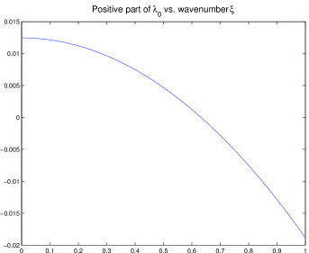
(a) (b)

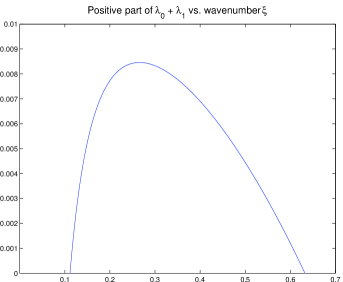
Figure 1: Positive part of the (a) $\lambda_{0}$ and (b) $\lambda_{0}+\lambda_{1}$ vs. wave number $\xi$ for $\delta=0.2$.

The curve attains its maximum for a wave number $\xi\approx 0.27$. Thus, the linear theory predicts the wave length of the most unstable wave to be approximately $2\pi/0.27\approx 23.27$. On an interval of length 100, we expect the formation of 4-5 clusters. This is in agreement with our numerical result shown in Section 7, Figure 3.

5 The quasi-dynamic approximation

In [6], we derived various systems of evolution equations describing the macroscopic behavior of the system (2) for intermediate and long times. We considered rectilinear flows in the direction of gravity with the rod orientations taking values on the sphere $S^{2}$ and derived the so called quasi-dynamic approximation (cf [6]). When one restricts to a shear flow in the direction of gravity

$$\boldsymbol{u}=(0,0,w(t,x))^{T}\,,\qquad f=f(t,x,\boldsymbol{n}),\quad\boldsymbol{n}\in S^{2}$$

and set $D_{r}=1$ we obtain the system consisting of an advection-diffusion equation coupled to a diffusion equation,

$$\begin{split}&\partial_{t}\rho(t,x)=\frac{1}{30}\partial_{x}\left[\frac{42^{2}}{42^{2}+46w_{x}^{2}}\left(\rho w_{x}+\frac{1}{3}\partial_{x}\rho\right)\right]\\ &Re\,\partial_{t}w(t,x)=\partial_{xx}w+\delta\left(\bar{\rho}-\rho\right).\end{split}$$ (18)

This model belongs to the class of flux-limited Keller-Segel systems and enjoyes gradient-flow structure (see [6]). The derivation of (18) is quite technical due to the complex form of the moment equations (and their closures) reflecting the structure of harmonic polynomials in dimension $d>2$.

To shed some light on the derivation of (18), we consider the simplified shear flow model (3), where now the rigid-rods are constrained to move in-plane, $\boldsymbol{n}\in S^{1}$, and present a derivation of the quasi-dynamic approximation. The idea behind the quasi-dynamic approximation is that the transient dynamics of the second order moments $c$ and $s$ is replaced by its equilibrium response, i.e. by

$$\begin{split}4D_{r}c+w_{x}s&=0\\ -\frac{1}{8}\partial_{x}\rho-\frac{1}{4}w_{x}\rho-w_{x}c+4D_{r}s&=0.\end{split}$$ (19)

System (19) can be solved for $s$, to obtain

$$s=\frac{D_{r}w_{x}\rho+\frac{1}{2}D_{r}\partial_{x}\rho}{16D_{r}^{2}+w_{x}^{2}}.$$ (20)

Inserting (20) into the first equation of (5), we obtain the quasi-dynamic approximation

$$\begin{split}\partial_{t}\rho&=\partial_{x}\left(\frac{D_{r}w_{x}}{16D_{r}^{2}+w_{x}^{2}}\rho\right)+\frac{1}{2}D_{r}\partial_{x}\left(\frac{1}{16D_{r}^{2}+w_{x}^{2}}\partial_{x}\rho\right)\\ Re\partial_{t}w&=\partial_{xx}w+\delta\left(\bar{\rho}-\rho\right).\end{split}$$ (21)

For the special case $D_{r}=1$ it gives

$$\begin{split}\partial_{t}\rho&=\partial_{x}\left(\frac{1}{16+w_{x}^{2}}\left(w_{x}\rho+\frac{1}{2}\partial_{x}\rho\right)\right)\\ Re\partial_{t}w&=\partial_{xx}w+\delta\left(\bar{\rho}-\rho\right).\end{split}$$ (22)

A comparison of (22) with (18) shows that we obtain the same general structure of a flux-limited Keller-Segel model. The simplification, which restricts the director to $S^{1}$, just leads to different constants.

6 The diffusive scaling

The diffusive scaling provides another approach for obtaining a macroscopic evolution equation for $\rho$. Here we present a direct derivation of the diffusive scaling for the simplified shear flow model (3), where we assume that the director $f$ only takes values on $S^{1}$. Again we restrict our considerations to the case $D_{r}=1$.

We consider (3) and rescale the model in the diffusive scale, i.e.

$$x=\frac{1}{\delta}\hat{x},\,t=\frac{1}{\delta^{2}}\hat{t},\,\boldsymbol{u}=\hat{\boldsymbol{u}}.$$

The scaled equations (dropping the hats and for $D_{r}=1$) have the form

$$\begin{split}&\delta^{2}\,\partial_{t}f(t,x,\theta)+\delta\,\partial_{\theta}\left(w_{x}\cos^{2}\theta f\right)-\delta\partial_{x}\left(\sin\theta\cos\theta f\right)=\partial_{\theta\theta}f\\ &Re\,\delta^{2}\,\partial_{t}w(t,x)=\delta^{2}\,\partial_{xx}w+\delta\left(\bar{\rho}-\int_{0}^{2\pi}f\,d\theta\right).\end{split}$$ (23)

Now we introduce the ansatz

$$\begin{split}f(t,x,\theta)&=\delta f_{0}+\delta^{2}f_{1}+\ldots\\ \boldsymbol{u}&=\boldsymbol{u}_{0}+\delta\boldsymbol{u}_{1}+\ldots=\left(\begin{array}[]{c}0\\ w_{0}\end{array}\right)+\delta\left(\begin{array}[]{c}0\\ w_{1}\end{array}\right)+\ldots\\ \bar{\rho}&=\delta\bar{\rho}_{0}\end{split}$$

and obtain the relations

$$O(\delta)\quad \partial_{\theta\theta}f_{0}=0$$ (24)

$$O(\delta^{2})\qquad \partial_{\theta}\left(w_{x}\cos^{2}\theta f_{0}\right)-\partial_{x}\left(\sin\theta\cos\theta f_{0}\right)=\partial_{\theta\theta}f_{1}$$ (25)

$$Re\partial_{t}w_{0}=\partial_{xx}w_{0}+\left(m-\int_{0}^{2\pi}f_{0}d\theta\right)$$

$$O(\delta^{3})\qquad \partial_{t}f_{0}+\partial_{\theta}\left(w_{x}\cos^{2}\theta f_{1}\right)-\partial_{x}\left(\sin\theta\cos\theta f_{1}\right)=\partial_{\theta\theta}f_{2}.$$ (26)

The relation (24) implies that $f_{0}$ depends at most linearly on $\theta$. As a function on $S^{1}$, $f$ is periodic. Thus, $f_{0}$ must be constant in $\theta$ and

$$\rho_{0}(t,x)=\int_{0}^{2\pi}f_{0}(t,x)d\theta=2\pi f_{0}(t,x).$$

Now we integrate equation (26) over $S^{1}$. The second and the last term vanish and we obtain

$$\partial_{t}\rho_{0}-\partial_{x}\int_{0}^{2\pi}\cos\theta\sin\theta f_{1}\,d\theta=0.$$

Using integration by parts, we arrive at

$$\begin{split}\partial_{t}\rho_{0}&=-\frac{1}{4}\partial_{x}\left(\int_{0}^{2\pi}\partial_{\theta\theta}\left(\cos\theta\sin\theta\right)f_{1}\,d\theta\right)\\ &=-\frac{1}{4}\partial_{x}\left(\int_{0}^{2\pi}\cos\theta\sin\theta\,\partial_{\theta\theta}f_{1}\,d\theta\right).\end{split}$$

Using (25), we replace $\partial_{\theta\theta}f_{1}$ by terms which depend on $f_{0}$ and obtain an evolution equation for $\rho_{0}$.

$$\begin{split}\partial_{t}\rho_{0}&=-\frac{1}{4}\partial_{x}\left(\int_{0}^{2\pi}\cos\theta\sin\theta\left[\partial_{\theta}\left(w_{x}\cos^{2}\theta f_{0}\right)-\partial_{x}\left(\sin\theta\cos\theta f_{0}\right)\right]\,d\theta\right)\\ &=\frac{1}{4\pi}\,\partial_{x}\left(w_{x}\rho_{0}\int_{0}^{2\pi}\cos^{2}\theta\sin^{2}\theta\,d\theta\right)+\frac{1}{8\pi}\partial_{x}\left((\partial_{x}\rho_{0})\int_{0}^{2\pi}\cos^{2}\theta\sin^{2}\theta\,d\theta\right)\\ &=\frac{1}{16}\partial_{x}\left(w_{x}\rho_{0}\right)+\frac{1}{32}\partial_{xx}\rho_{0}\end{split}$$

Thus, in the diffusive limit, the dynamics of the simplified shear flow problem (3) is described by the system

$$\begin{split}\partial_{t}\rho&=\frac{1}{16}\partial_{x}\left(w_{x}\rho+\frac{1}{2}\partial_{x}\rho\right)\\ Re\,\partial_{t}w&=\partial_{xx}w+\left(\bar{\rho}-\rho\right).\end{split}$$ (27)

In Appendix A.2, we derive the diffusive scaling for the kinetic model (1) in the case of rectilinear flow for rigid rods that move in $S^{2}$. For shear flow and in the special case $D_{r}=1$, $\gamma=0$, the diffusive scaling of (2) leads to the model equation

$$\begin{split}\partial_{t}\rho&=\frac{1}{30}\partial_{x}\left(w_{x}\rho+\frac{1}{3}\partial_{x}\rho\right)\\ Re\partial_{t}w&=\partial_{xx}w+\left(\bar{\rho}-\rho\right).\end{split}$$ (28)

Again we obtain a Keller-Segel type model. In contrast to the quasi-dynamic approximation, the diffusive scaling does not provide flux limiting.

7 Numerical simulations

In this section we show numerical simulations for shear flow, which compare the simplified shear flow model (3) with the quasi-dynamic approximation (18) and the diffusive scaling (27). In Figure 2 we show results of numerical simulations using the parameter values $D_{r}=\delta=Re=1$. The initial values are set to be

$$\begin{split}\rho(x_{k},0)&=1+10^{-4}\left(\epsilon(x_{k})-\frac{1}{2}\right)\\ w(x_{k},0)&=0,\end{split}$$ (29)

where $\epsilon(x_{k})$ is a random number between $0$ and $1$. We impose the periodicity condition on an interval of length $100$. For our test simulations we used $800$ grid cells in space, thus $k=1,\ldots,800$. In the simulation of the full model, $S^{1}$ is discretized with $200$ grid cells. We observe the formation of clusters with higher particle density.

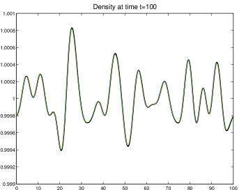
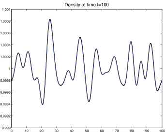
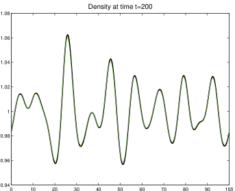
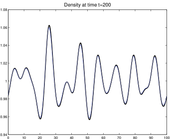
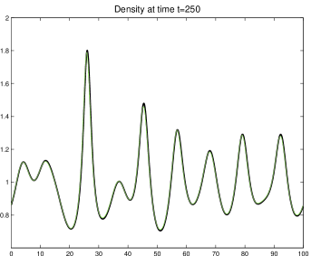
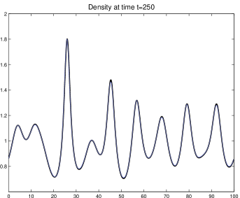
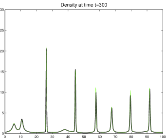
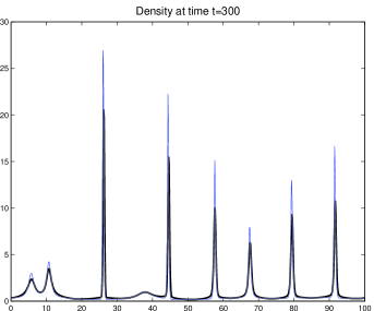
Figure 2: Left plots: Comparison of the quasi-dynamic approximation (green line) with the full model (black line). Right plots: Comparison of the diffusive scaling (blue line) with the full model (black line).

Both the solutions predicted by the quasi-dynamic approximation as well as the solutions predicted by the diffusive limit compare very well with the solution structure obtained by the full model. Only at a very late times, some differences can be observed and the quasi-dynamic approximation leads to slightly more accurate results.

Note that the model equations obtained by the quasi-dynamic approximation contain the same non-dimensional parameters as the full model. For the diffusive limit this is not the case, since the parameter $\delta$ does no longer appear in (27). In Figure 3 we show simulations comparing the quasi-dynamic approximation with the full model for $\delta=0.2$, using the same initial conditions as above.

In order to simulate this problem with the diffusive model, we impose periodic boundary conditions on a domain of length $\delta 100=20$ and consider numerical approximations for $t\leq\delta^{2}2000=80$. Furthermore, we set initial values as described by (29) but multiplied by $1/\delta$. Finally we used $\bar{\rho}=1/\delta$ in equation (27). To compare the numerical solution of the diffusive limit system with the solution of the full model, we map the numerical solution to the interval $[0,100]$ and multiply with $\delta$. The results are shown in Figure 3 on the right hand side.

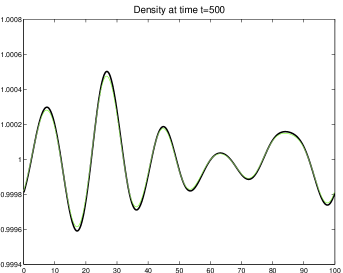
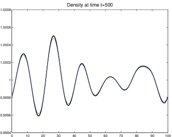
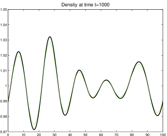
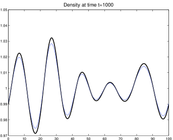
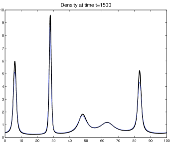
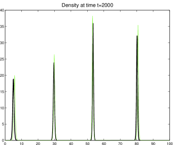
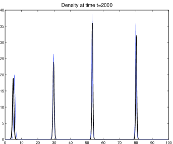
Figure 3: Left plots: Comparison of the quasi-dynamic approximation (green line) with the full model (black line). Right plots: Comparison of the diffusive scaling (blue line) with the full model (black line). The simulations correspond to $\delta=0.2$.

At later times the cluster start to merge. This coarsening behavior can be observed with all of the three models. Here a better agreement is observed for the quasi-dynamic approximation, see Figure 4.

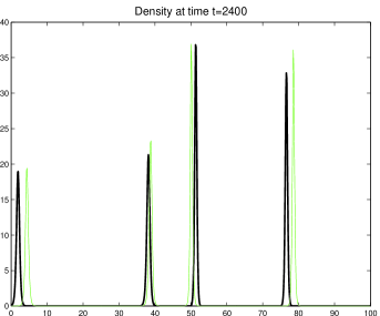
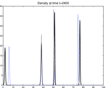
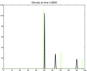
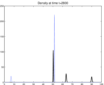
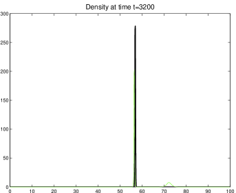
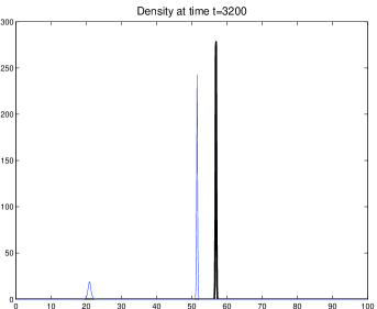
Figure 4: Results of a simulation with $\delta=0.2$ at later times. Left plots: Comparison of the quasi-dynamic approximation (green line) with the full model (black line). Right plots: Comparison of the diffusive scaling (blue line) with the full model (black line).

Conclusions

Based on a simplified kinetic model, we have studied the sedimentation of rod-like particles under the influence of gravity. Linear stability shows both instability of a well stirred initial configuration as well as a wave length selection mechanism for a non-zero Reynolds number. We presented two models describing the macroscopic response of the system. One of these models, the quasi-dynamic approximation, is obtained from a moment closure system using the assumption that the evolution equation of the second order moments can be replaced by an equilibrium relation. The resulting macroscopic system has the form of a flux-limited Keller-Segel model. Another macroscopic model is obtained by taking the diffusive limit of the kinetic model. In this case we obtain a standard Keller-Segel type model. Numerical computations confirm good agreement of the predicted solution structure of both macroscopic models compared to the kinetic model. For very long times the quasi-dynamic approximation shows a better agreement with the original kinetic model.

Finally, it is interesting to note the differences of the macroscopic models depending on whether the orientation of the rod-like particles is a function on $S^{1}$ or $S^{2}$, respectively. The macroscopic models which are derived from the simplified kinetic model are less diffusive than those which are derived from the more general kinetic model.

Appendix A Collective behavior in scaling limits

In this appendix we derive the hyperbolic and diffusive limits for the system (1). The description of collective behavior of kinetic models through hyperbolic or parabolic limits is well known in several contexts in fluid dynamics or biological transport systems (e.g. [3, 11, 12]). The novelty here is that the kinetic variable takes values in the sphere, what requires some special calculations detailed in this appendix.

It is expedient to view the scaling limits from the perspective of describing the aggregate behavior of a suspension. The function

$$\rho(t,\boldsymbol{x})=\int_{S^{d-1}}f(t,\boldsymbol{x},\boldsymbol{n})d\boldsymbol{n}$$

measures the density of rod-like particles. Linear stability theory predicts an instability for the quiescent solution; it is then natural to calculate the aggregate response of the system in long times. To this end, we proceed to calculate the hyperbolic and diffusive limits. It turns out that the limiting behavior in the hyperbolic scaling will be described by a Boussinesq type system. For certain flows the hyperbolic scaling produces a trivial behavior, and it is then natural to consider the diffusive scaling. Such a situation occurs for two-dimensional rectilinear flows of suspensions, where we will show that the collective behavior in the diffusive limit is described by the Keller-Segel model.

A.1 The hyperbolic scaling

We first rescale the model (1) in the hyperbolic scaling,

$$\boldsymbol{x}=\frac{1}{\delta}\hat{\boldsymbol{x}},\ t=\frac{1}{\delta}\hat{t},\ \boldsymbol{u}=\hat{\boldsymbol{u}},\ p=\hat{p}.$$

The scaled equations (after dropping the hats) are

$$\delta\partial_{t}f+\delta\boldsymbol{u}\cdot\nabla_{\boldsymbol{x}}f -\delta D(\boldsymbol{n})\boldsymbol{e}_{2}\cdot\nabla_{\boldsymbol{x}}f+\delta\nabla_{\boldsymbol{n}}\cdot\left(P_{\boldsymbol{n}^{\bot}}\nabla_{\boldsymbol{x}}\boldsymbol{u}\boldsymbol{n}f\right)$$ (30)

$$=\Delta_{\boldsymbol{n}}f+\delta^{2}\gamma\nabla_{\boldsymbol{x}}\cdot D(\boldsymbol{n})\nabla_{\boldsymbol{x}}f$$

$$Re\,\delta\,\left(\partial_{t}\boldsymbol{u}+\left(\boldsymbol{u}\cdot\nabla_{\boldsymbol{x}}\right)\boldsymbol{u}\right)-\delta^{2}\Delta_{\boldsymbol{x}}\boldsymbol{u} +\delta\nabla_{\boldsymbol{x}}p-\delta^{2}\gamma\nabla_{\boldsymbol{x}}\cdot\sigma=\delta\left(\bar{\rho}-\int_{S^{2}}fd\boldsymbol{n}\right)\boldsymbol{e}_{3}$$

$$\qquad\qquad\delta\nabla_{\boldsymbol{x}}\cdot\boldsymbol{u}=0$$

where $D(\boldsymbol{n})=I+\boldsymbol{n}\otimes\boldsymbol{n}$.

We introduce the ansatz

$$\begin{split}f&=f_{0}+\delta f_{1}+\ldots\\ \boldsymbol{u}&=\boldsymbol{u}_{0}+\delta\boldsymbol{u}_{1}+\ldots\\ p&=p_{0}+\delta p_{1}+\ldots\end{split}$$

to the system (30) and obtain equations for the various orders of the expansion:

$$O(1)\quad \Delta_{\boldsymbol{n}}f_{0}=0$$ (31)

$$O(\delta)\quad \partial_{t}f_{0}+\boldsymbol{u}_{0}\cdot\nabla_{\boldsymbol{x}}f_{0}-D(\boldsymbol{n})\boldsymbol{e}_{2}\cdot\nabla_{\boldsymbol{x}}f_{0}+\nabla_{\boldsymbol{n}}\cdot\left(P_{\boldsymbol{n}^{\bot}}\nabla_{\boldsymbol{x}}\boldsymbol{u}_{0}\boldsymbol{n}f_{0}\right)=\Delta_{\boldsymbol{n}}f_{1}$$ (32)

$$O(\delta)\quad Re\,\left(\partial_{t}\boldsymbol{u}_{0}+\left(\boldsymbol{u}_{0}\cdot\nabla_{\boldsymbol{x}}\right)\boldsymbol{u}_{0}\right)+\nabla_{\boldsymbol{x}}p_{0}=\Big{(}\bar{\rho}-\int_{S^{2}}f_{0}d\boldsymbol{n}\Big{)}\boldsymbol{e}_{3}$$

$$O(1)\quad \nabla_{\boldsymbol{x}}\cdot\boldsymbol{u}_{0}=0$$

It follows from (31) that $f_{0}$ is independent of $\boldsymbol{n}$ and thus

$$f_{0}(t,\boldsymbol{x},\boldsymbol{n})=\frac{1}{4\pi}\int_{S^{2}}f_{0}d\boldsymbol{n}=\frac{1}{4\pi}\rho_{0}(t,\boldsymbol{x})$$

Then integrating (32) over the sphere, we deduce that $\rho_{0}=\int_{S^{2}}f_{0}d\boldsymbol{n}$ and $\boldsymbol{u}_{0}$ satisfy the Boussinesq system

$$\partial_{t}\rho_{0}+\nabla_{\boldsymbol{x}}\cdot\left(\boldsymbol{u}_{0}\rho_{0}-\big{(}\frac{1}{4\pi}\int_{S^{2}}D(\boldsymbol{n})d\boldsymbol{n}\big{)}\boldsymbol{e}_{2}\rho_{0}\right) =0$$ (33)

$$Re\,\left(\partial_{t}\boldsymbol{u}_{0}+\left(\boldsymbol{u}_{0}\cdot\nabla_{\boldsymbol{x}}\right)\boldsymbol{u}_{0}\right)+\nabla_{\boldsymbol{x}}p_{0} =(\bar{\rho}-\rho_{0})\boldsymbol{e}_{3}$$

$$\nabla_{\boldsymbol{x}}\cdot\boldsymbol{u}_{0} =0$$

The constant $\bar{\rho}$ can be absorbed into the pressure, by redefining $p_{0}$ to account for the hydrostatic pressure, that is by setting $p_{0}=\hat{p}_{0}+\bar{\rho}\boldsymbol{x}\cdot\boldsymbol{e}_{3}$.

A.2 The diffusive scaling

Next, we confine to rectilinear flows with a vertical velocity field obeying the ansatz

$$\boldsymbol{u}(t,x,y)=(0,0,w(t,x,y))^{T}\;,\quad f=f(t,x,y)$$ (34)

and depending only on the horizontal variables. The flow cross section is the domain $D$ and we assume that the boundary conditions are either periodic or no-slip. This restriction to the two-dimensional case is motivated by experimental observations of long clusters with higher particle density. We note that for this ansatz the nonlinear transport terms $u\cdot\nabla f$ and $(u\cdot\nabla)u$ drop out.

One checks that under the ansatz (34) the system (33) reduces to the trivial problem

$$\partial_{t}\rho_{0}=0,\quad Re\,\partial_{t}w_{0}=(\bar{\rho}-\rho_{0})\,,\quad p_{0}=-\bar{\rho}z$$

which can be easily solved in terms of the initial data. The objective then becomes to calculate the next order correction in the diffusive scale.

We return to (1), note that for the ansatz (34) the nonlinear convective terms $u\cdot\nabla f$ and $(u\cdot\nabla)u$ drop out, and rescale the model in the diffusive scaling, i.e.

$$\boldsymbol{x}=\frac{1}{\delta}\hat{\boldsymbol{x}},\ t=\frac{1}{\delta^{2}}\hat{t},\ \boldsymbol{u}=\hat{\boldsymbol{u}},\ p=\hat{p}.$$ (35)

The scaled equations (after dropping the hats) have the form

$$\begin{split}\delta^{2}\partial_{t}f-\delta D(\boldsymbol{n})\boldsymbol{e}_{3}\cdot\nabla_{\boldsymbol{x}}f+\delta\nabla_{\boldsymbol{n}}\cdot\left(P_{\boldsymbol{n}^{\bot}}\nabla_{\boldsymbol{x}}\boldsymbol{u}\boldsymbol{n}f\right)&=D_{r}\Delta_{\boldsymbol{n}}f+\delta^{2}\gamma\nabla_{\boldsymbol{x}}\cdot D(\boldsymbol{n})\nabla_{\boldsymbol{x}}f\\ \delta^{2}\,Re\,\partial_{t}\boldsymbol{u}+\delta\nabla_{\boldsymbol{x}}p&=\delta^{2}\Delta_{\boldsymbol{x}}\boldsymbol{u}+\delta^{2}\gamma\nabla_{\boldsymbol{x}}\cdot\sigma+\delta\Big{(}\bar{\rho}-\int_{S^{2}}fd\boldsymbol{n}\Big{)}\boldsymbol{e}_{3}\\ \nabla_{\boldsymbol{x}}\cdot\boldsymbol{u}&=0\end{split}$$

We introduce the ansatz

$$\begin{split}f(t,x,y,\boldsymbol{n})&=\delta f_{0}+\delta^{2}f_{1}+\ldots\\ \boldsymbol{u}(t,x,y)&=\boldsymbol{u}_{0}+\delta\boldsymbol{u}_{1}+\ldots=\left(\begin{array}[]{c}0\\ 0\\ w_{0}\end{array}\right)+\delta\left(\begin{array}[]{c}0\\ 0\\ w_{1}\end{array}\right)+\ldots\\ p&=\delta p_{0}+\delta^{2}p_{1}+\ldots\\ \bar{\rho}&=\delta\bar{\rho}_{0}+\delta^{2}\bar{\rho}_{1}+\ldots\end{split}$$ (36)

to the above system and collect the terms of the same order, arriving at

$$O(\delta)\quad \Delta_{\boldsymbol{n}}f_{0}=0$$ (37)

$$O(\delta^{2})\qquad -D(\boldsymbol{n})\boldsymbol{e}_{3}\cdot\nabla_{\boldsymbol{x}}f_{0}+\nabla_{\boldsymbol{n}}\cdot\left(P_{\boldsymbol{n}^{\bot}}\nabla_{\boldsymbol{x}}\boldsymbol{u}_{0}\boldsymbol{n}f_{0}\right)=D_{r}\Delta_{\boldsymbol{n}}f_{1}$$ (38)

$$O(\delta^{3})\quad \partial_{t}f_{0}-D(\boldsymbol{n})\boldsymbol{e}_{3}\cdot\nabla_{\boldsymbol{x}}f_{1}+\nabla_{\boldsymbol{n}}\cdot\left(P_{\boldsymbol{n}^{\bot}}\big{(}\nabla_{\boldsymbol{x}}\boldsymbol{u}_{1}\boldsymbol{n}f_{0}+\nabla_{\boldsymbol{x}}\boldsymbol{u}_{0}\boldsymbol{n}f_{1}\big{)}\right)$$

$$\qquad\qquad=D_{r}\Delta_{\boldsymbol{n}}f_{2}+\gamma\nabla_{\boldsymbol{x}}\cdot D(\boldsymbol{n})\nabla_{\boldsymbol{x}}f_{0}$$ (39)

The same procedure applied to the Stokes system yields

$$O(\delta)\qquad \nabla_{\boldsymbol{x}}\cdot\boldsymbol{u}_{0}=0$$

$$O(\delta^{2})\qquad \partial_{t}\boldsymbol{u}_{0}+\nabla_{\boldsymbol{x}}p_{0}=\Delta_{\boldsymbol{x}}\boldsymbol{u}_{0}+\left(\bar{\rho}_{0}-\int_{S^{2}}f_{0}d\boldsymbol{n}\right)\boldsymbol{e}_{3}$$ (40)

We want to derive an evolution equation for $\rho_{0}$ and $w_{0}$. In order to do this, we first summarise a few tools. Recall that $\boldsymbol{n}\in S^{2}$ has the form

$$\boldsymbol{n}=\left(\begin{array}[]{c}\sin\theta\cos\phi\\ \sin\theta\sin\phi\\ \cos\theta\end{array}\right),\quad 0\leq\theta<\pi,\,0\leq\phi<2\pi.$$

Furthermore, recall that the components of the tensor $3\boldsymbol{n}\otimes\boldsymbol{n}-{\rm id}$ are the surface spherical harmonics of order 2. This means, they are harmonic polynomials on $\mathbb{R}^{3}$ of order 2, restricted to $S^{2}$. The surface spherical harmonics are eigenfunctions of the Laplacian on $S^{2}$ with corresponding eigenvalue $-\ell(\ell+1)$, where $\ell$ is the order [1, App. E]. Hence

$$\triangle_{\boldsymbol{n}}(3\,n_{i}\,n_{j}-\delta_{ij})\;=\;-6\,(3\,n_{i}\,n_{j}-\delta_{ij}).$$ (41)

Finally, note that for any $3\times 3$ matrix $\kappa$, the equation

$$\nabla_{\boldsymbol{n}}\cdot\left(P_{\boldsymbol{n}^{\bot}}\kappa\boldsymbol{n}\right)=\mbox{tr }\kappa-3\boldsymbol{n}\cdot\kappa\boldsymbol{n}\,,$$ (42)

holds, where tr stands for the trace operator. Also, using symmetries of $S^{2}$, we obtain the formula

$$\frac{1}{4\pi}\int_{S^{2}}\boldsymbol{n}\otimes\boldsymbol{n}d\boldsymbol{n}=\tfrac{1}{3}I.$$ (43)

Now we are ready to derive an evolution equation for $\rho_{0}$. Equation (37) implies that $f_{0}$ is independent on $\boldsymbol{n}$, that is

$$f_{0}=\frac{1}{4\pi}\int_{S^{2}}f_{0}d\boldsymbol{n}=\frac{1}{4\pi}\rho_{0}(t,x,y)$$

Next, integration of (39) over the sphere and use of (43) and the fact that $e_{3}\cdot\nabla_{x}f_{1}=0$ for our ansatz gives that $\rho_{0}$ satisfies

$$\partial_{t}\rho_{0}=\nabla_{\boldsymbol{x}}\cdot\underbrace{\int_{S^{2}}\left(D(\boldsymbol{n})-\frac{1}{4\pi}\int_{S^{2}}D(\boldsymbol{n})d\boldsymbol{n}\right)\boldsymbol{e}_{3}f_{1}\,d\boldsymbol{n}}_{=:I_{1}}+\gamma\nabla_{\boldsymbol{x}}\cdot\underbrace{\frac{1}{4\pi}\int_{S^{2}}D(\boldsymbol{n})d\boldsymbol{n}\,}_{=:I_{2}}\nabla_{\boldsymbol{x}}\rho_{0}$$ (44)

where the terms $I_{1}$ and $I_{2}$ are computed in terms of $f_{1}$ solving (38) for $f_{0}=\frac{1}{4\pi}\rho_{0}$.

It remains to compute the terms $I_{1}$ and $I_{2}$. Observe now that we have the identities:

$$\int_{S^{2}}(\boldsymbol{n}\otimes\boldsymbol{n}-\frac{1}{3}I)d\boldsymbol{n} \stackrel{{\scriptstyle\eqref{surfhar}}}{{=}}-\frac{1}{6}\int_{S^{2}}\triangle_{\boldsymbol{n}}(\boldsymbol{n}\otimes\boldsymbol{n}-\frac{1}{3}I)d\boldsymbol{n}=0$$

$$I_{2}:=\frac{1}{4\pi}\int_{S^{2}}D(\boldsymbol{n})d\boldsymbol{n} =\frac{1}{4\pi}\int_{S^{2}}(\boldsymbol{n}\otimes\boldsymbol{n}+I)d\boldsymbol{n}=\frac{4}{3}I$$ (45)

$$D(\boldsymbol{n})-\frac{1}{4\pi}\int_{S^{2}}D(\boldsymbol{n})d\boldsymbol{n} =\boldsymbol{n}\otimes\boldsymbol{n}-\frac{1}{3}I$$

These, in conjunction with (37), (38) and (42), imply that $f_{1}$ satisfies

$$\Delta_{\boldsymbol{n}}f_{1} =-\big{(}D(\boldsymbol{n})-\frac{1}{4\pi}\int_{S^{2}}D(\boldsymbol{n})d\boldsymbol{n}\big{)}\boldsymbol{e}_{3}\cdot\frac{1}{4\pi}\nabla_{\boldsymbol{x}}\rho_{0}+\frac{1}{4\pi}\nabla_{\boldsymbol{n}}\cdot\left(P_{\boldsymbol{n}^{\bot}}\nabla_{\boldsymbol{x}}\boldsymbol{u}_{0}\boldsymbol{n}\right)\rho_{0}$$

$$=-\big{(}\boldsymbol{n}\otimes\boldsymbol{n}-\frac{1}{3}I\big{)}\boldsymbol{e}_{3}\cdot\frac{1}{4\pi}\nabla_{\boldsymbol{x}}\rho_{0}-\frac{3}{4\pi}\rho_{0}(\boldsymbol{n}\cdot\nabla_{\boldsymbol{x}}\boldsymbol{u}_{0}\boldsymbol{n})$$ (46)

Next, we compute $I_{1}$

$$\begin{split}I_{1}&:=\int_{S^{2}}\left(D(\boldsymbol{n})-\frac{1}{4\pi}\int_{S^{2}}D(\boldsymbol{n})d\boldsymbol{n}\right)\boldsymbol{e}_{3}f_{1}\,d\boldsymbol{n}\\ &=\int_{S^{2}}\big{(}\boldsymbol{n}\otimes\boldsymbol{n}-\frac{1}{3}I\big{)}\boldsymbol{e}_{3}f_{1}d\boldsymbol{n}\\ &\stackrel{{\scriptstyle\eqref{surfhar}}}{{=}}-\frac{1}{6}\int_{S^{2}}\triangle_{\boldsymbol{n}}\big{(}\boldsymbol{n}\otimes\boldsymbol{n}-\frac{1}{3}I\big{)}\boldsymbol{e}_{3}f_{1}d\boldsymbol{n}\\ &\stackrel{{\scriptstyle\eqref{as4}}}{{=}}\frac{1}{24\pi}\int_{S^{2}}\big{(}\boldsymbol{n}\otimes\boldsymbol{n}-\frac{1}{3}I\big{)}\boldsymbol{e}_{3}\Big{[}\big{(}\boldsymbol{n}\otimes\boldsymbol{n}-\frac{1}{3}I\big{)}\boldsymbol{e}_{3}\cdot\nabla_{\boldsymbol{x}}\rho_{0}+3\rho_{0}(\boldsymbol{n}\cdot\nabla_{\boldsymbol{x}}\boldsymbol{u}_{0}\boldsymbol{n})\Big{]}d\boldsymbol{n}\\ &=\frac{1}{24\pi}\int_{S^{2}}\left(\begin{array}[]{c}n_{1}n_{3}\\ n_{2}n_{3}\\ n_{3}^{2}-\frac{1}{3}\end{array}\right)\Big{[}(3\rho_{0}w_{0x}+\rho_{0x})n_{1}n_{3}+(3\rho_{0}w_{0y}+\rho_{0y})n_{2}n_{3}\Big{]}d\boldsymbol{n}\end{split}$$

Observe that, due to symmetry considerations, the integrals

$$\int_{S^{2}}n_{1}n_{3}^{3}-\frac{1}{3}n_{1}n_{3}d\boldsymbol{n} =0$$

$$\int_{S^{2}}n_{2}n_{3}^{3}-\frac{1}{3}n_{2}n_{3}d\boldsymbol{n} =0$$

$$\int_{S^{2}}n_{1}n_{2}n_{3}^{2}d\boldsymbol{n}= =0,$$

while the remaining integrals are computed via spherical coordinates

$$\int_{S^{2}}n_{1}^{2}n_{3}^{2}d\boldsymbol{n} =\int_{0}^{\pi}\sin^{3}\theta\cos^{2}\theta\,d\theta\int_{0}^{2\pi}\cos^{2}\varphi d\varphi=\frac{4\pi}{15}$$

$$\int_{S^{2}}n_{2}^{2}n_{3}^{2}d\boldsymbol{n} =\int_{0}^{\pi}\sin^{3}\theta\cos^{2}\theta\,d\theta\int_{0}^{2\pi}\sin^{2}\varphi d\varphi=\frac{4\pi}{15}.$$

We conclude that

$$I_{1}=\frac{1}{90}\left(3\rho_{0}w_{0x}+\rho_{0x}\,,\;3\rho_{0}w_{0y}+\rho_{0y}\,,0\;\right)^{T}$$

and that $\rho_{0}$ satisfies the equation

$$\partial_{t}\rho_{0} =\frac{1}{30}\left(\partial_{x}\left(\frac{1}{3}\rho_{0x}+\rho_{0}w_{0x}\right)+\partial_{y}\left(\frac{1}{3}\rho_{0y}+\rho_{0}w_{0y}\right)\right)+\gamma\frac{4}{3}\Delta_{(x,y)}\rho_{0}$$

$$=\frac{1}{30}\nabla_{(x,y)}\cdot\big{(}\rho_{0}\nabla_{(x,y)}w_{0}\big{)}+\frac{1}{3}\left(4\gamma+\frac{1}{30}\right)\triangle_{(x,y)}\rho_{0}$$

Finally, we want to derive the evolution equation for $w_{0}$. From (40) we obtain

$$\partial_{x}p_{0}=\partial_{y}p_{0}=0$$

and

$$Re\partial_{t}w_{0}-\Delta_{(x,y)}w_{0}+\partial_{z}p_{0}=(\bar{\rho}_{0}-\rho_{0})$$ (47)

The ansatz (36) implies that the right hand side of (47) depends only on $(x,y)$. Thus we deduce that the pressure has the form $p=\kappa(t)z$, where $\kappa$ is arbitrary and reflects the effect of an imposed pressure gradient. If there is no imposed pressure gradient then the pressure is hydrostatic and $\bar{\rho}_{0}=\tfrac{1}{|D|}\int_{D}\rho(t,x,y)dxdy$ which is conserved. In the following we restrict our considerations to the case $\gamma=0$. The functions $(\rho_{0},w_{0})$ are selected by solving the coupled system

$$\begin{split}\partial_{t}\rho_{0}&=\frac{1}{30}\nabla_{(x,y)}\cdot\left(\rho\nabla_{(x,y)}w_{0}\right)+\frac{1}{90}\Delta_{(x,y)}\rho_{0}\\ Re\,\partial_{t}w_{0}&=\Delta_{(x,y)}w_{0}+(\bar{\rho}-\rho_{0}),\end{split}$$ (48)

where $\bar{\rho}$ is (as above) the average density.

References

- [1] R.B. Bird, Ch.F. Curtiss, R.C. Armstrong, and O. Hassager. Dynamics of Polymeric Liquids, Vol. 2, Kinetic Theory. Wiley Interscience, 1987.
- [2] J.-A. Carillo, Th. Goudon and P. Lafitte. Simulation of fluid and particles flows: Asymptotic preserving schemes for bubbling and flowing regimes. J. Comput. Physics, 227 (2008) 7929-7951.
- [3] F.A.C.C. Chalub, P.A. Markowich, B. Perthame, and C. Schmeiser. Kinetic models for chemotaxis and their drift-diffusion limits. Monatsh. Math., 142 (2004), 123–141.
- [4] M. Doi and S.F. Edwards. The Theory of Polymer Dynamics. Oxford University Press, 1986.
- [5] É. Guazzelli and J. Hinch. Fluctuations and instability in sedimentation. Annu. Rev. Fluid Mech., 42 (2011), 97-116.
- [6] Ch. Helzel and A.E. Tzavaras. A kinetic model for the sedimentation of rod-like particles. 2015 (submitted).
- [7] B. Herzhaft and É. Guazzelli. Experimental study of the sedimentation of a dilute fiber suspension. Physical Review Letters, 77 (1996), 290-293.
- [8] B. Herzhaft and É. Guazzelli. Experimental study of the sedimentation of dilute and semi-dilute suspensions of fibers. J. Fluid Mech., 384 (1999), 133-158.
- [9] D.L. Koch and E.S.G. Shaqfeh. The instability of a dispersion of sedimenting spheroids. J. Fluid Mech., 209 (1989), 521-542.
- [10] B. Metzger, J.E. Butlerz and É. Guazzelli. Experimental investigation of the instability of a sedimenting suspension of fibers. J. Fluid Mech., 575 (2007), 307-332.
- [11] H.G. Othmer and T. Hillen. The diffusion limit of transport equations II: Chemotaxis equations. SIAM J. Appl. Math. 62 (2002), 1222-1250.
- [12] F. Poupaud and J. Soler. Parabolic limit and stability of the Vlasov-Poisson-Fokker-Planck system. Math. Mod. Meth. Appl. Sci. 10 (2000), 1027 1045.