Nonlinear memory capacity of parallel time-delay reservoir computers in the processing of multidimensional signals

Abstract

This paper addresses the reservoir design problem in the context of delay-based reservoir computers for multidimensional input signals, parallel architectures, and real-time multitasking. First, an approximating reservoir model is presented in those frameworks that provides an explicit functional link between the reservoir parameters and architecture and its performance in the execution of a specific task. Second, the inference properties of the ridge regression estimator in the multivariate context is used to assess the impact of finite sample training on the decrease of the reservoir capacity. Finally, an empirical study is conducted that shows the adequacy of the theoretical results with the empirical performances exhibited by various reservoir architectures in the execution of several nonlinear tasks with multidimensional inputs. Our results confirm the robustness properties of the parallel reservoir architecture with respect to task misspecification and parameter choice that had already been documented in the literature.

Key Words: Reservoir computing, echo state networks, liquid state machines, time-delay reservoir, parallel computing, memory capacity, multidimensional signals processing, Big Data.

1 Introduction

The recent and fast development of numerous massive data acquisition technologies results in a considerable growth of the data volumes that are stored and that need to be processed in the context of many human activities. The variability, complexity, and volume of this information have motivated the appearance of the generic term Big Data, which is mainly used to refer to datasets whose features make the traditional data processing approaches inadequate. This relatively new concept calls for the development of specialized tools for data preprocessing, analysis, transferring, and visualization, as well as for novel data mining and machine learning techniques in order to tackle specific computational tasks.

In this context, there is a recent but already well established paradigm for neural computation known by the name of reservoir computing (RC) [Jaeg 01, Jaeg 04, Maas 02, Maas 11, Croo 07, Vers 07, Luko 09] (also referred to as Echo State Networks and Liquid State Machines), that has already shown a significant potential in successfully confronting some of the challenges that we just described.

This brain-inspired machine learning methodology exhibits several competitive advantages with respect to more traditional approaches. First, the supervised learning scheme associated to it is extremely simple. Second, some implementations of the RC paradigm are based on the computational capacities of certain dynamical systems [Crut 10] that open the door to physical realizations that have already been built using dedicated hardware (see, for instance, [Jaeg 07, Atiy 00, Appe 11, Roda 11, Larg 12, Paqu 12]) and that, recently, have shown unprecedented information processing speeds [Brun 13]. Our work takes place in the context of this specific type of RCs and, more explicitly, in the so called time-delay reservoirs (TDRs) that use the sampling of the solutions of time-delay differential equations in the construction of the RC.

Despite the outstanding empirical performances of TDRs described in the above listed references and the convenience of the learning scheme associated to them, a well-known important drawback is that these devices show a certain lack of structural task universality. More specifically, each task presented to a TDR requires that the TDR parameters and, more generally, its architecture are tuned in order to achieve optimal performance or, equivalently, small deviations from the optimal parameter values can seriously degrade the reservoir performance. The optimal parameters have been traditionally found by trial and error or by running costly numerical scannings for each task. More recently, in [Grig 15a] we introduced a method to overcome this difficulty by providing a functional link between the RC parameters and its performance with respect to a given task and that can be used to accurately determine the optimal reservoir architecture by solving a well structured optimization problem; this feature simplifies enormously the implementation effort and sheds new light on the mechanisms that govern this information processing technique.

This paper builds on the techniques introduced in [Grig 15a] and extends those results in the following directions:

(i)

The memory capacity formulas in [Grig 15a] are generalized to multidimensional input signals and we provide capacity estimations for the simultaneous execution of several memory tasks. This feature, sometimes referred to as real-time multitasking [Maas 11] is usually presented as one of the most prominent computational advantages of RC.

(ii)

We provide memory capacity estimations for parallel arrays of reservoir computers. This reservoir architecture has been introduced in [Orti 12, Grig 14] and has been empirically shown to exhibit improved robustness properties with respect to the dependence of the optimal reservoir parameters on the task presented to the device and also with respect to task misspecification.

(iii)

We carry out an in-depth study of the ridge regression estimator in the multivariate context in order to assess the impact of finite sample training on the decrease of reservoir capacity. More specifically, when the teaching signal used to train the RC has finite size, the faulty estimation of the RC readout layer (see Section 2.2) introduces an error that is cumulated with the characteristic error associated to the RC scheme and that we explicitly quantify.

(iv)

We conduct an empirical study that shows the adequacy of our theoretical results with the empirical performances exhibited by TDRs in the execution of various nonlinear tasks with multidimensional inputs. Additionally, we confirmed using the approximating model, the robustness properties of the parallel reservoir architecture with respect to task misspecification and parameter choice that had already been documented in [Grig 14].

The paper is organized as follows: Section 2 recalls the general setup for time-delay reservoir computing, as well as the notions of characteristic error and memory capacity in the multitasking setup. Section 3 constitutes the core of the paper and addresses the points (i) through (iii) listed in the previous paragraphs. The empirical study described in point (iv) is contained in Section 4.

Acknowledgments: We acknowledge partial financial support of the Région de Franche-Comté (Convention 2013C-5493), the European project PHOCUS (FP7 Grant No. 240763), the ANR “BIPHOPROC” project (ANR-14-OHRI-0002-02), and Deployment S.L. LG acknowledges financial support from the Faculty for the Future Program of the Schlumberger Foundation.

2 Notation and preliminaries

In this section we introduce the notation that we use in the paper, we briefly recall the general setup for time-delay reservoirs (TDRs), and provide various preliminary concepts that are needed in the following sections.

2.1 Notation

Column vectors are denoted by bold lower or upper case symbol like $\mathbf{v}$ or $\mathbf{V}$. We write $\mathbf{v}^{\top}$ to indicate the transpose of $\mathbf{v}$. Given a vector $\mathbf{v}\in\mathbb{R}^{n}$, we denote its entries by $v_{i}$, with $i\in\left\{1,\dots,n\right\}$; we also write $\mathbf{v}=(v_{i})_{i\in\left\{1,\dots,n\right\}}$. The symbols $\mathbf{i}_{n}$ and $\mathbf{0}_{n}$ stand for the vectors of length $n$ consisting of ones and zeros, respectively. We denote by $\mathbb{M}_{n,m}$ the space of real $n\times m$ matrices with $m,n\in\mathbb{N}$. When $n=m$, we use the symbol $\mathbb{M}_{n}$ to refer to the space of square matrices of order $n$. Given a matrix $A\in\mathbb{M}_{n,m}$, we denote its components by $A_{ij}$ and we write $A=(A_{ij})$, with $i\in\left\{1,\dots,n\right\}$, $j\in\left\{1,\dots m\right\}$. We write $\mathbb{I}_{n}$ and $\mathbb{O}_{n}$ to denote the identity matrix and the zero matrix of dimension $n$, respectively. We use $\mathbb{S}_{n}$ to indicate the subspace $\mathbb{S}_{n}\subset\mathbb{M}_{n}$ of symmetric matrices, that is, $\mathbb{S}_{n}=\left\{A\in\mathbb{M}_{n}\mid A^{\top}=A\right\}$. Given a matrix $A\in\mathbb{M}_{n,m}$, we denote by vec the operator that transforms $A$ into a vector of length $nm$ by stacking all its columns, namely,

$${\rm vec}:\mathbb{M}_{n,m}\longrightarrow\mathbb{R}^{nm},\quad{\rm vec}\left(A\right)=\left(A_{11},\dots,A_{n1},\dots,A_{1m},\dots,A_{nm}\right)^{\top},\quad A\in\mathbb{M}_{n,m}.$$

When $A$ is symmetric, we denote by vech the operator that stacks the elements on and below the main diagonal of $A$ into a vector of length $N:=\frac{1}{2}n\left(n+1\right)$, that is,

$${\rm vech}:\mathbb{S}_{n}\longrightarrow\mathbb{R}^{N},\quad{\rm vech}\left(A\right)=\left(A_{11},\dots,A_{n1},A_{22},\dots,A_{n2},\dots,A_{nn}\right)^{\top},\quad A\in\mathbb{S}_{n}.$$

Let $N:=\frac{1}{2}n\left(n+1\right)$. We denote by $L_{n}\in\mathbb{M}_{N,n^{2}}$ and by $D_{n}\in\mathbb{M}_{n^{2},N}$ the elimination and the duplication matrices [Lutk 05], respectively. These matrices satisfy that:

$${\rm vech}\left(A\right)=L_{n}{\rm vec}\left(A\right),\quad\mbox{and}\quad{\rm vec}\left(A\right)=D_{n}{\rm vech}\left(A\right).$$ (2.1)

Consider $A\in\mathbb{S}_{n}$, $\mathbf{v}={{\rm vech}}\left(A\right)\in\mathbb{R}^{N}$, and $S=\left\{\left(i,j\right)|i,j\in\left\{1,\dots,n\right\},i\geq j\right\}$. Let $\sigma:S\longrightarrow\left\{1,\dots,N\right\}$ be the operator that assigns to the position of the entry $\left(i,j\right)$, $i\geq j$, of the matrix $A$ the position of the corresponding element of $\mathbf{v}$ in the ${\rm vech}$ representation. We refer to the inverse of this operator as ${{\sigma}^{-1}}:\left\{1,\dots,N\right\}\longrightarrow S$. The symbol $||A||_{\rm Frob}$ denotes the Frobenius norm of $A\in\mathbb{M}_{m,n}$ defined as $\|A\|_{{\rm Frob}}^{2}:={\rm trace}\left(A^{T}A\right)$ [Meye 00]. Finally, the symbols ${\rm E}[\cdot]$, ${\rm var}(\cdot)$, and ${\rm Cov}(\cdot,\cdot)$ denote the mathematical expectation, the variance, and the covariance, respectively.

2.2 The general setup for time-delay reservoir (TDR) computing

The functional time-delay differential equations used for TDR computing. The time-delay reservoirs studied in this paper are constructed by sampling the solutions of time-delay differential equations of the form

$$\dot{x}(t)=-x(t)+f(x(t-\tau),I(t),\boldsymbol{\theta}),$$ (2.2)

where $f$ is a nonlinear smooth function that will be referred to as nonlinear kernel, $\boldsymbol{\theta}\in\mathbb{R}^{K}$ is a vector that contains the parameters of the nonlinear kernel, $\tau>0$ is the delay, $x(t)\in\mathbb{R}$, and $I(t)\in\mathbb{R}$ is an external forcing that makes (2.2) non-autonomous and that in our construction will be used as an inlet into the system for the signal that needs to be processed. We emphasize that the solution space of equation (2.2) is infinite dimensional since an entire function $x\in C^{1}([-\tau,0],\mathbb{R})$ needs to be specified in order to initialize it. The nonlinear kernel $f$ is chosen based on the concrete physical implementation of the computing system that is envisioned. We consider two specific parametric sets of kernels that have already been explored in the literature, namely:

(i)

The Mackey-Glass [Mack 77] nonlinear kernel:

$$f(x,I,\boldsymbol{\theta})=\frac{\eta\left(x+\gamma I\right)}{1+\left(x+\gamma I\right)^{p}},\enspace\boldsymbol{\theta}:=(\gamma,\eta,p)\in\mathbb{R}^{3},$$ (2.3)

which is used in electronics-based RC implementations [Appe 11].

(ii)

The Ikeda [Iked 79] nonlinear kernel

$$f(x,I,\boldsymbol{\theta})=\eta\sin^{2}\left(x+\gamma I+\phi\right),\enspace\boldsymbol{\theta}:=(\eta,\gamma,\phi)\in\mathbb{R}^{3},$$ (2.4)

associated to the optical RC implementations [Larg 12].

For these specific choices of nonlinear kernel, the parameters $\gamma$ and $\eta$ are usually referred to as the input and feedback gains, respectively.

Continuous and discrete-time approaches to multidimensional TDR computing. We briefly recall the design of a TDR using the solutions of (2.2). The following constructions are discussed in detail in [Grig 15a]. TDRs are based on the sampling of the solutions of (2.2) when driven by an input forcing obtained out of the signal that needs to be processed. More specifically, let ${\bf z}(t)\in\mathbb{R}^{n}$, $t\in\mathbb{Z}$, be an $n$-dimensional discrete-time input signal. This signal is, first, time and dimensionally multiplexed over a delay period by using an input mask $C\in\mathbb{M}_{N,n}$ and by setting $\mathbf{I}(t):=C{\bf z}(t)$, $t\in\mathbb{Z}$, where $N$ is a design parameter called the number of neurons of each reservoir layer. The resulting discrete-time $N$-dimensional signal $\mathbf{I}(t)\in\mathbb{R}^{N}$ is called input forcing.

We now consider two different constructions of the TDR depending on the way in which the solutions of the time-delay differential equation (2.2) are handled. The continuous time TDR is constructed as a collection of neuron values $x_{i}(t)$ organized in layers $\mathbf{x}(t)\in\mathbb{R}^{N}$ of $N\in\mathbb{N}$ of virtual neurons each, parameterized by $t\in\mathbb{Z}$. The value $x_{i}(t)$, referred to as the $i$th neuron value of the $t$th layer $\mathbf{x}(t)$ of the reservoir, is obtained by sampling a solution $x(t)$ of (2.2) by setting

$$x_{i}(t):=x(t\tau-(N-i)d),\quad i\in\{1,\ldots,N\},\quad t\in\mathbb{Z},$$ (2.5)

where $d:=\tau/N$ is referred to as the separation between neurons. The solution $x(t)$ has been obtained by using an external forcing $I(s)$ in (2.2) constructed out of the input forcing $\mathbf{I}(t)$ as follows: given $s\in\mathbb{R}$, let $t\in\mathbb{Z}$ and $i\in\{2,\ldots,N\}$ be the unique values such that $s\in(t\tau-(N-i-1)d,t\tau-(N-i)d]$ and that we use to define the external forcing as $I(s):=(\mathbf{I}(t))_{i}$.

The discrete-time TDR is constructed via the Euler time-discretization of (2.2) with an integration step of $d:=\tau/N$. In this case, the neuron values are determined by the following recursions:

$$x_{i}(t):=e^{-\xi}x_{i-1}(t)+(1-e^{-\xi})f(x_{i}(t-1),({\bf I}(t))_{i},\boldsymbol{\theta}),$$ (2.6)

with $x_{0}(t):=x_{N}(t-1)$, $\xi:=\log(1+d)$, and $i\in\left\{1,\dots,N\right\}$. In this case, the recursions (2.6) uniquely determine a smooth map $F:\mathbb{R}^{N}\times\mathbb{R}^{N}\times\mathbb{R}^{K}\rightarrow\mathbb{R}^{N}$ referred to as the reservoir map that specifies the neuron values of a given $t$th layer as a recursion on the neuron values of the preceding layer $t-1$ via an expression of the form

$$\mathbf{x}(t)=F(\mathbf{x}(t-1),\mathbf{I}(t),\boldsymbol{\theta}).$$ (2.7)

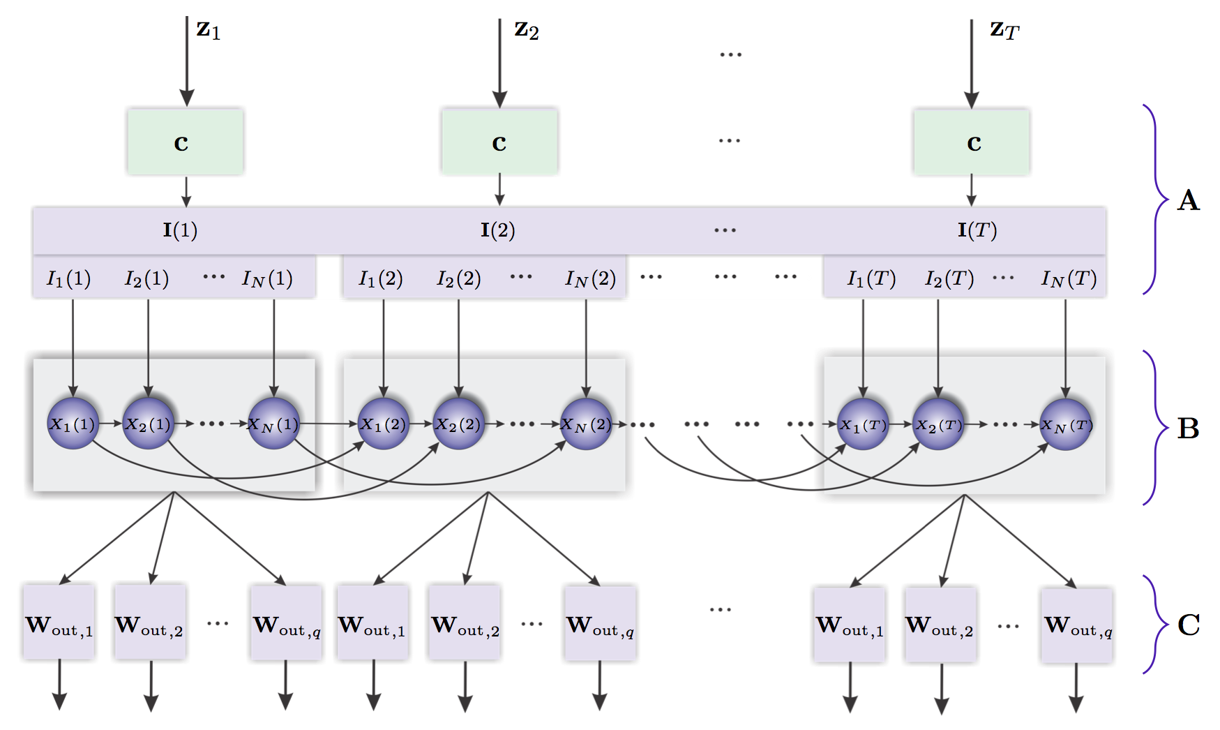
Figure 1: Diagram representing the architecture of a TDR reservoir with a multitask readout. The module A is the input layer, B is a neural diagram representing the discrete-time reservoir dynamics implied by equation (2.6), and C is the multitask readout layer in which each column of the matrix $W_{{\rm out}}$ accomplishes a different task based on the same reservoir output.

The TDR memory capacity for real-time multitasking. In this paper we study the performance of TDRs at the time of simultaneously performing several memory tasks (see Figure 1). This means that we will evaluate the ability of the TDR to reproduce a prescribed multidimensional nonlinear function of the input signal

$$\begin{array}[]{cccc}H:&\mathbb{R}^{(h+1)n}&\longrightarrow&\mathbb{R}^{q}\\ &{\rm vec}({\bf z}(t),\dots,{\bf z}(t-h))&\longmapsto&\mathbf{y}(t),\end{array}$$ (2.10)

that we will call $q$-dimensional $h$-lag memory task for the $n$-dimensional input signal $\left\{{\bf z}(t)\right\}_{t\in\mathbb{Z}}$.

In the RC context, this task is performed by using a finite size realization of the input signal $\{{\bf z}(-h+1),\ldots,{\bf z}(T)\}$ that is used to construct a $q$-dimensional teaching signal $\{{\bf y}(1),\ldots,{\bf y}(T)\}$ by setting ${\bf y}(t):=H\left({\rm vec}({\bf z}(t),\dots,{\bf z}(t-h))\right)$. The teaching signal is subsequently used to determine a pair $\left({W}_{{\rm out}},\boldsymbol{a}_{\rm out}\right)\in\mathbb{M}_{N,q}\times\mathbb{R}^{q}$ that performs the memory task as an affine combination of the reservoir outputs. The optimal pair $\left({W}_{{\rm out}},\boldsymbol{a}_{\rm out}\right)$ is obtained with a ridge regression that minimizes the regularized square error, that is,

$$({W}_{{\rm out}},\boldsymbol{a}_{\rm out}) =\mathop{\rm arg\,min}_{{W}\in\mathbb{M}_{N,q},\boldsymbol{a}\in\mathbb{R}^{q}}\left({\rm trace}\left({\rm E}\left[({W}^{\top}\cdot{\bf x}(t)+\boldsymbol{a}-\mathbf{y}(t))^{\top}({W}^{\top}\cdot{\bf x}(t)+\boldsymbol{a}-\mathbf{y}(t))\right]\right)+\lambda\|{W}\|^{2}_{\rm Frob}\right)$$ (2.11)

$$=:\mathop{\rm arg\,min}_{{W}\in\mathbb{M}_{N,q},\boldsymbol{a}\in\mathbb{R}^{q}}\left({\rm MSE}(W,\boldsymbol{a})+\lambda\|{W}\|^{2}_{\rm Frob}\right).$$ (2.12)

The optimal pair $({W}_{{\rm out}},\boldsymbol{a}_{\rm out})$ that solves the ridge regression problem (2.12) is referred to as the readout layer. The ridge regularization parameter $\lambda\in\mathbb{R}$ is usually tuned during the training phase via cross-validation. The explicit solution of the optimization problem (2.12) (see [Grig 15a] for the details) is given by

$${W}_{\rm out}= (\Gamma(0)+\lambda\mathbb{I}_{N})^{-1}{\rm Cov}(\mathbf{x}(t),\mathbf{y}(t)),$$ (2.13)

$$\boldsymbol{a}_{\rm out}= \boldsymbol{\mu}_{y}-{W}_{\rm out}^{\top}\boldsymbol{\mu}_{x},$$ (2.14)

where $\boldsymbol{\mu}_{x}:={\rm E}[\mathbf{x}(t)]\in\mathbb{R}^{N}$, $\boldsymbol{\mu}_{y}:={\rm E}[\mathbf{y}(t)]\in\mathbb{R}^{q}$, $\Gamma(0):={\rm Cov}(\mathbf{x}(t),\mathbf{x}(t))\in\mathbb{S}_{N}$, and ${\rm Cov}(\mathbf{x}(t),\mathbf{y}(t))\in\mathbb{M}_{N,q}$. Stationarity hypotheses are assumed on the teaching signal and the reservoir output so that the first and second order moments that we just listed are time-independent. The error committed by the reservoir when accomplishing the task $H$ with the optimal readout will be referred to as its characteristic error and is given by the expression

$${\rm MSE}(W_{{\rm out}},\boldsymbol{a}_{{\rm out}})={\rm trace}({\rm Cov}\left(\mathbf{y}(t),\mathbf{y}(t)\right)-{W}_{{\rm out}}^{\top}(\Gamma(0)+2\lambda\mathbb{I}_{N}){W}_{{\rm out}}),$$ (2.15)

that can be encoded under the form of a memory capacity $C_{H}(\boldsymbol{\theta},C,\lambda)$ with values between zero and one that depends on the task $H$ that is being tackled, the input mask $C$, the reservoir parameters $\boldsymbol{\theta}$ and the regularization constant $\lambda$:

$$C_{H}(\boldsymbol{\theta},C,\lambda):= 1-\dfrac{{\rm MSE}(W_{{\rm out}},\boldsymbol{a}_{{\rm out}})}{{\rm trace}\left({\rm Cov}(\mathbf{y}(t),\mathbf{y}(t))\right)}=\dfrac{{\rm trace}({W}_{{\rm out}}^{\top}(\Gamma(0)+2\lambda\mathbb{I}_{N}){W}_{{\rm out}})}{{\rm trace}\left({\rm Cov}(\mathbf{y}(t),\mathbf{y}(t))\right)},$$ (2.16)

where $W_{\rm out}$ is provided by the solution in (2.13). In order to evaluate (2.16) for a specific memory task, the expressions of $\Gamma(0)$, ${\rm Cov}(\mathbf{x}(t),\mathbf{y}(t))$, and ${\rm Cov}(\mathbf{y}(t),\mathbf{y}(t))$ need to be computed. The matrix $\Gamma(0)$ depends exclusively on the input signal and the reservoir architecture but ${\rm Cov}(\mathbf{y}(t),\mathbf{y}(t))$ and ${\rm Cov}(\mathbf{x}(t),\mathbf{y}(t))$ are related to the specific memory task $H$ at hand. The computation of (2.16) is in general very complicated and that is why in [Grig 15a] we introduced a simplified reservoir model that allowed us to efficiently evaluate it for one-dimensional statistically independent input signals and memory tasks. The extension of this theoretical tool to a multidimensional setup and to parallel architectures is one of the main goals of this paper.

Finally, there are situations in which the moments $\boldsymbol{\mu}_{x}$, $\boldsymbol{\mu}_{y}$, $\Gamma(0)$, and ${\rm Cov}(\mathbf{x}(t),\mathbf{y}(t))$, necessary to compute the readout layer $({W}_{{\rm out}},\boldsymbol{a}_{\rm out})$ using the equations (2.13)-(2.14), are obtained directly out of finite sample realizations of the teaching signal and of the reservoir output. The use in that context of finite sample empirical estimators carries in its wake an additional error that adds up to the characteristic error (2.15) and that we study later on in Section 3.4.

3 Reservoir memory capacities for parallel architectures and for multidimensional input signals and tasks

In this section we generalize the reservoir model proposed in [Grig 15a] in order to accommodate the treatment of multidimensional input signals and the computation of memory capacities associated to the execution of several simultaneous memory tasks, as well as the performance evaluation of parallel reservoir architectures. The main virtue of the reservoir model is that it allows for the explicit computation of the different elements that constitute the capacity formula (2.16) making hence accessible its evaluation.

In the last section we study the dependence of the reservoir performance on the length of the teaching signal and the regularization regression parameter. In particular we formulate asymptotic expressions that provide an estimation of the added error that is commited in memory tasks when the training is incomplete due to the finiteness of the training sample.

The reservoir model introduced in [Grig 15a] is based on the observation that optimal reservoir performance is frequently attained when the reservoir is functioning in a neighborhood of an asymptotically stable equilibrium of the autonomous system associated to (2.2). This feature suggests the possibility of approximating the reservoir by its partial linearization at that stable fixed point with respect to the delayed self feedback but keeping the nonlinearity at the level of the input signal injection. This observation motivated in [Grig 15a] an in-depth study of the stability properties of the equilibria $x_{0}$ of the time-delay differential equation (2.2) and of the corresponding fixed points $\mathbf{x}_{0}=x_{0}\mathbf{i}_{N}\in\mathbb{R}^{N}$ of the discrete-time approximation (2.7), both considered in the autonomous regime, that is, when $I(t)=0$ in (2.2) and $\mathbf{I}(t)={\bf 0}_{N}$ in (2.7), respectively. In particular, it was shown that (see Corollary D.5 and Theorem D.10 in the Supplementary Material in [Grig 15a]) that $|\partial_{{x}}f({x}_{0},{0},\boldsymbol{\theta})|<1$ is a sufficient condition for the asymptotic stability of $x_{0}\in\mathbb{R}$ and $\mathbf{x}_{0}=x_{0}\mathbf{i}_{N}\in\mathbb{R}^{N}$ in the continuous and discrete-time cases, respectively, which given a particular kernel $f$ allows for the identification of specific regions in parameter space in which stability is guaranteed (see Corollaries D.6 and D.7 of the Supplementary Material in [Grig 15a] for the Mackey-Glass and Ikeda kernel cases).

3.1 The reservoir model for multidimensional input signals

Consider a discrete-time TDR described by a reservoir map $F:\mathbb{R}^{N}\times\mathbb{R}^{N}\times\mathbb{R}^{K}\rightarrow\mathbb{R}^{N}$ as in (2.7). Let $\mathbf{x}_{0}\in\mathbb{R}^{N}$ be a stable fixed point of the autonomous systems associated to (2.7), that is, $F({\bf x}_{0},{\bf 0}_{N},\boldsymbol{\theta})={\bf x}_{0}$. In order to write down the approximate reservoir model as in [Grig 15a] we start by approximating (2.7) by its partial linearization at $\mathbf{x}_{0}$ with respect to the delayed self feedback and by the $R$th-order Taylor series expansion on the input forcing $\mathbf{I}(t)\in\mathbb{R}^{N}$. We obtain the following expression:

$$\mathbf{x}(t)=F(\mathbf{x}_{0},{\bf 0}_{N},\boldsymbol{\theta})+A(\mathbf{x}_{0},\boldsymbol{\theta})(\mathbf{x}(t-1)-\mathbf{x}_{0})+\boldsymbol{\varepsilon}(t),$$ (3.1)

where $F(\mathbf{x}_{0},{\bf 0}_{N},\boldsymbol{\theta})$ is the reservoir map evaluated at the point $(\mathbf{x}_{0},{\bf 0}_{N},\boldsymbol{\theta})$ and $A(\mathbf{x}_{0},\boldsymbol{\theta}):=D_{\mathbf{x}}F(\mathbf{x}_{0},{\bf 0}_{N},\boldsymbol{\theta})$ is the first derivative of $F$ with respect to its first argument, computed at the point $(\mathbf{x}_{0},{\bf 0}_{N},\boldsymbol{\theta})$. The vector $\boldsymbol{\varepsilon}(t)\in\mathbb{R}^{N}$, $t\in\mathbb{Z}$, in (3.1) is obtained out of the Taylor series expansion of $F(\mathbf{x}(t),\mathbf{I}(t),\boldsymbol{\theta})$ in (2.7) on $\mathbf{I}(t)$ up to some fixed order $R\in\mathbb{N}$. For each $r\in\left\{1,\dots,N\right\}$ its $r$th component can be written as

$${\varepsilon}_{r}(t)=(1-{e}^{-\xi})\sum^{R}_{i=1}\dfrac{1}{i!}(\partial_{{I}}^{(i)}f)({x}_{0},0,\boldsymbol{\theta})\sum^{r}_{j=1}e^{-(r-j)\xi}I_{j}(t)^{i},$$ (3.2)

where $(\partial_{{I}}^{(i)}f)({x}_{0},0,\boldsymbol{\theta})$ is the $i$th order partial derivative of the nonlinear reservoir kernel map $f$ in (2.2) with respect to the second argument $I(t)$ computed at the point $({x}_{0},0,\boldsymbol{\theta})$. Finally, $A(\mathbf{x}_{0},\boldsymbol{\theta})$ is called the connectivity matrix of the reservoir at the point $\mathbf{x}_{0}$ and has the following explicit form

$$A(\mathbf{x}_{0},\boldsymbol{\theta})={\small\left(\begin{array}[]{cccccc}\Phi&0&\ldots&0&{e^{-\xi}{}}\\ {e^{-\xi}}\Phi&\Phi&\ldots&0&{e^{-2\xi}{}}\\ e^{-2\xi}\Phi&e^{-\xi}\Phi&\ldots&0&{e^{-3\xi}{}}\\ \vdots&\vdots&\ddots&\vdots&\vdots\\ e^{-(N-1)\xi}\Phi&e^{-(N-2)\xi}\Phi&\ldots&{e^{-\xi}}{}\Phi&\Phi+{e^{-N\xi}{}}\end{array}\right)},$$ (3.8)

where $\Phi:=(1-e^{-\xi})\partial_{x}f(x_{0},0,\boldsymbol{\theta})$ and $\partial_{x}f(x_{0},0,\boldsymbol{\theta})$ is the first derivative of the nonlinear kernel $f$ in (2.2) with respect to the first argument and computed at the point $(x_{0},0,\boldsymbol{\theta})$.

Suppose now that the input signal is a collection of $n$-dimensional independent and identically distributed random variables $\left\{{\bf z}(t)\right\}_{t\in\mathbb{Z}}\sim{\rm IID}({\bf 0}_{n},\Sigma_{z})$, $\Sigma_{z}\in\mathbb{S}^{+}_{n}$, and that we take as input mask the matrix $C\in\mathbb{M}_{N,n}$. Since for each ${t\in\mathbb{Z}}$ the input forcing $\mathbf{I}(t)\in\mathbb{R}^{N}$ is constructed via the assignment $\mathbf{I}(t):=C{\bf z}(t)$ we have that $\left\{\mathbf{I}(t)\right\}_{t\in\mathbb{Z}}\sim{\rm IID}({\bf 0}_{N},\Sigma_{I})$, with $\Sigma_{I}:=C\Sigma_{z}C^{\top}$. It follows then that $I_{j}(t)=\sum^{n}_{k=1}C_{jk}z_{k}(t)$ which substituted in (3.2) yields that

$$\boldsymbol{\varepsilon}(t)=(1-{e}^{-\xi})\left(\begin{array}[]{c}V_{R}\left({\bf z}(t),\left\{C_{1,\cdot}\right\},x_{0},\boldsymbol{\theta}\right)\\ V_{R}\left({\bf z}(t),\left\{C_{j,\cdot}\right\}_{j\in\left\{1,2\right\}},x_{0},\boldsymbol{\theta}\right)\\ \vdots\\ V_{R}\left({\bf z}(t),\left\{C_{j,\cdot}\right\}_{j\in\left\{1,\dots,N\right\}},x_{0},\boldsymbol{\theta}\right)\end{array}\right),$$ (3.9)

with the polynomials

$$V_{R}\left({\bf z}(t),\left\{C_{j,\cdot}\right\}_{j\in\left\{1,\dots,r\right\}},x_{0},\boldsymbol{\theta}\right) :=\sum^{R}_{i=1}(\partial_{{I}}^{(i)}f)({x}_{0},0,\boldsymbol{\theta})\sum^{r}_{j=1}{e}^{-(r-j)\xi}\sum_{k_{1}+\dots+k_{n}=i}\dfrac{1}{k_{1}!\dots k_{n}!}\prod^{n}_{s=1}C_{js}^{k_{s}}\cdot\prod^{n}_{s=1}z_{s}(t)^{k_{s}}.$$ (3.10)

The symbol $\left\{C_{j,\cdot}\right\}$, $j\in\left\{1,\dots N\right\}$, denotes the set of all the entries in the $j$th row of the input mask matrix $C$. The assumption $\left\{{\bf z}(t)\right\}_{t\in\mathbb{Z}}\sim{\rm IID}({\bf 0}_{n},\Sigma_{z})$ implies that $\{\boldsymbol{\varepsilon}(t)\}_{t\in\mathbb{Z}}$ is also a family of $N$-dimensional independent and identically distributed random variables with mean $\boldsymbol{\mu}_{{\varepsilon}}$ and covariance matrix $\Sigma_{{\varepsilon}}$ given by

$$(\boldsymbol{\mu}_{{\varepsilon}})_{r}=(1-{e}^{-\xi})\sum^{R}_{i=1}(\partial_{{I}}^{(i)}f)({x}_{0},0,\boldsymbol{\theta})\sum^{r}_{j=1}e^{-(r-j)\xi}\sum_{k_{1}+\dots+k_{n}=i}\dfrac{1}{k_{1}!\dots k_{n}!}\prod^{n}_{s=1}C_{js}^{k_{s}}\cdot\mu_{k_{1},\dots,k_{n}}({\bf z}),$$ (3.11)

where

$$\mu_{k_{1},\dots,k_{n}}({\bf z}(t)):={\rm E}\left[\prod^{n}_{s=1}z_{s}(t)^{k_{s}}\right]$$ (3.12)

denotes a higher-order moment of ${\bf z}(t)\in\mathbb{R}^{n}$ whose existence we assume for values $k_{1},\dots,k_{n}$ such that $k_{1}+\cdots+k_{n}\leq 2R$. Additionally, $\Sigma_{{\varepsilon}}:={\rm E}\left[(\boldsymbol{\varepsilon}(t)-\boldsymbol{\mu}_{{\varepsilon}})(\boldsymbol{\varepsilon}(t)-\boldsymbol{\mu}_{{\varepsilon}})^{\top}\right]$ has entries determined by the relation:

$$(\Sigma_{{\varepsilon}})_{rs}=(1-{e}^{-\xi})^{2}{\rm E} \left[V_{R}\left({\bf z}(t),\left\{C_{j,\cdot}\right\}_{j\in\left\{1,\dots,r\right\}},x_{0},\boldsymbol{\theta}\right)\cdot V_{R}\left({\bf z}(t),\left\{C_{j,\cdot}\right\}_{j\in\left\{1,\dots,s\right\}},x_{0},\boldsymbol{\theta}\right)\right]$$

$$-(\boldsymbol{\mu}_{\boldsymbol{\varepsilon}})_{r}(\boldsymbol{\mu}_{\boldsymbol{\varepsilon}})_{s},\quad r,s\in\left\{1,\dots,N\right\},$$ (3.13)

where the first summand is computed by first multiplying the polynomials $V_{R}\left({\bf z},\left\{C_{j,\cdot}\right\}_{j\in\left\{1,\dots,r\right\}},x_{0},\boldsymbol{\theta}\right)$ and $V_{R}\left({\bf z},\left\{C_{j,\cdot}\right\}_{j\in\left\{1,\dots,s\right\}},x_{0},\boldsymbol{\theta}\right)$ on the variable ${\bf z}\in\mathbb{R}^{n}$ and subsequently evaluating the resulting polynomial according to the following convention: any monomial of the form $az_{1}^{k_{1}}\cdots z_{n}^{k_{n}}$ is replaced by $a\mu_{k_{1},\dots,k_{n}}({\bf z})$.

A particular case in which the higher-order moments (3.12) can be readily computed is when $\left\{{\bf z}(t)\right\}_{t\in\mathbb{Z}}\sim{\rm IN}({\bf 0}_{n},\Sigma_{z})$, that is, $\left\{{\bf z}(t)\right\}_{t\in\mathbb{Z}}$ follows an $n$-dimensional multivariate normal distribution. Indeed, following [Holm 88, Tria 03], let $k_{1},\ldots,k_{n}\in\mathbb{N}$ be $n$ nonzero natural numbers such that $K:=k_{1}+k_{2}+\dots+k_{n}$ and let ${\bf z}^{\mathcal{K}}:=\left(z_{1}\mathbf{i}_{k_{1}}^{\top},z_{2}\mathbf{i}_{k_{2}}^{\top},\dots,z_{n}\mathbf{i}_{k_{n}}^{\top}\right)^{\top}\in\mathbb{R}^{K}$. The vector ${\bf z}^{\mathcal{K}}\in\mathbb{R}^{K}$ is Gaussian with zero mean and covariance matrix $\Sigma_{z}^{\mathcal{K}}\in\mathbb{S}_{K}$ given by $(\Sigma_{z}^{\mathcal{K}})_{ij}={\rm Cov}({z}_{i}^{\mathcal{K}},{z}_{j}^{\mathcal{K}})$, for any $i,j\in\left\{1,\dots,K\right\}$, that is, ${\bf z}^{\mathcal{K}}\sim{\rm IN}({\bf 0}_{K},\Sigma_{z}^{\mathcal{K}})$. Then, using Theorem 1 in [Tria 03], we can write that

$$\mu_{k_{1},\ldots,k_{n}}({\bf z})=\left\{\begin{array}[]{cl}Hf(\Sigma_{z}^{\mathcal{K}}),&{\rm when}\enspace K=2l,\quad l\in\mathbb{N},\\ &\\ 0,&{\rm otherwise},\end{array}\right.$$ (3.14)

where the symbol $Hf(\Sigma_{z}^{\mathcal{K}})$ denotes the hafnian of the covariance matrix $\Sigma_{z}^{\mathcal{K}}$ of order $2l$, $l\in\mathbb{N}$, defined by

$$Hf(\Sigma_{z}^{\mathcal{K}}):=\sum_{I,J}(\Sigma_{z}^{\mathcal{K}})_{i^{\prime}_{1}j^{\prime}_{1}}(\Sigma_{z}^{\mathcal{K}})_{i^{\prime}_{2}j^{\prime}_{2}}\cdots(\Sigma_{z}^{\mathcal{K}})_{i^{\prime}_{l}j^{\prime}_{l}},$$ (3.15)

where the sum is running over all the possible decompositions of $\left\{1,2,\dots,2l=K\right\}$ into disjoint subsets $I,J$ of the form $I=\left\{i^{\prime}_{1},\ldots,i^{\prime}_{l}\right\}$, $J=\left\{j^{\prime}_{1},\ldots,j^{\prime}_{l}\right\}$, such that $i^{\prime}_{1}<\cdots<i^{\prime}_{l}$, $j^{\prime}_{1}<\cdots<j^{\prime}_{l}$, and $i^{\prime}_{w}<j^{\prime}_{w}$, for each $w\in\{1,\ldots,l\}$.

We now proceed as in [Grig 15a] and consider (3.1) as a VAR(1) model [Lutk 05] driven by the independent noise $\{\boldsymbol{\varepsilon}(t)\}_{t\in\mathbb{Z}}$. If we assume that the nonlinear kernel $f$ satisfies the stability condition $|\partial_{{x}}f({x}_{0},{0},\boldsymbol{\theta})|<1$, then the proof of Theorem D.10 in [Grig 15a] shows that the spectral radius $\rho(A(\mathbf{x}_{0},\boldsymbol{\theta}))<1$, which implies in turn that (3.1) has a unique causal and second order stationary solution [Lutk 05, Proposition 2.1] $\{\mathbf{x}(t)\}_{t\in\mathbb{Z}}$ with time-independent mean

$$\boldsymbol{\mu}_{{x}}=(I_{N}-A(\mathbf{x}_{0},\boldsymbol{\theta}))^{-1}(F(\mathbf{x}_{0},{\bf 0}_{N},\boldsymbol{\theta})-A(\mathbf{x}_{0},\boldsymbol{\theta})\mathbf{x}_{0}+\boldsymbol{\mu}_{{\varepsilon}}).$$ (3.16)

The model (3.1) can hence be rewritten in mean-adjusted form as

$$\mathbf{x}(t)-\boldsymbol{\mu}_{{x}}=A(\mathbf{x}_{0},\boldsymbol{\theta})(\mathbf{x}(t-1)-\boldsymbol{\mu}_{{x}})+(\boldsymbol{\varepsilon}(t)-\boldsymbol{\mu}_{{\varepsilon}}).$$ (3.17)

Additionally, the autocovariance function $\Gamma(k):={\rm E}\left[\left(\mathbf{x}(t)-\boldsymbol{\mu}_{{x}}\right)\left(\mathbf{x}(t-k)-\boldsymbol{\mu}_{{x}}\right)^{\top}\right]$ at lag $k\in\mathbb{Z}$ is determined by the Yule-Walker equations [Lutk 05], which have the following solutions in vectorized form:

$${\rm vech}(\Gamma(0)) =\left(\mathbb{I}_{N^{\prime}}-L_{N}(A(\mathbf{x}_{0},\boldsymbol{\theta})\otimes A(\mathbf{x}_{0},\boldsymbol{\theta})\right))^{-1}{\rm vech}(\Sigma_{{\varepsilon}}),$$ (3.18)

$$\Gamma(k) =A(\mathbf{x}_{0},\boldsymbol{\theta})\Gamma(k-1)\enspace{\rm with}\enspace\Gamma(-k)=\Gamma(k)^{\top},$$ (3.19)

where $N^{\prime}:=\dfrac{1}{2}N(N+1)$ and $L_{N}\in\mathbb{M}_{N^{\prime},N^{2}}$, $D_{N}\in\mathbb{M}_{N^{2},N^{\prime}}$ are the elimination and the duplication matrices, respectively. We recall that the autocovariance function $\Gamma(0)$ is one of the key components of the capacity formula (2.16) that we intend to explicitly evaluate.

3.2 The reservoir model for parallel TDRs with multidimensional input signals

In this section we generalize the reservoir model that we just developed to the parallel time-delay reservoir architecture that introduced in [Orti 12, Grig 14]. This reservoir design has shown very satisfactory robustness properties with respect to model misspecification and parameter choice. The basic idea on which this approach is built consists of presenting the input signal to a parallel array of reservoirs, each of them running with different parameter values. The concatenation of the outputs of these reservoirs is then used to construct a single readout layer via a ridge regression. Figure 2 provides a diagram representing the parallel reservoir computing architecture.

\begin{overpic}[scale={0.37},tics=5]{plot2.png} \!\! \put(12.0,54.0){\large$C^{1}$} \put(42.0,54.0){\large$C^{2}$} \put(82.5,54.0){\large$C^{p}$} \put(2.2,29.5){$X^{1}_{1}(T)$} \put(9.5,29.5){$X^{1}_{2}(T)$} \put(21.0,29.5){$X^{1}_{N_{1}}(T)$} \par\par\put(31.3,29.5){$X^{2}_{1}(T)$} \put(38.3,29.5){$X^{2}_{2}(T)$} \put(50.3,29.5){$X^{2}_{N_{2}}(T)$} \par\put(72.3,30.0){$X^{p}_{1}(T)$} \put(79.3,30.0){$X^{p}_{2}(T)$} \put(91.4,30.0){$X^{p}_{N_{p}}(T)$} \par\put(15.3,39.0){\scriptsize$R(\boldsymbol{\theta}_{1},\lambda_{1})$} \put(44.7,39.0){\scriptsize$R(\boldsymbol{\theta}_{2},\lambda_{2})$} \put(85.0,39.0){\scriptsize$R(\boldsymbol{\theta}_{p},\lambda_{p})$} \par\put(16.0,65.0){$\mathbf{Z}$} \put(46.0,65.0){$\mathbf{Z}$} \put(86.0,65.0){$\mathbf{Z}$} \par\put(13.5,44.5){\large$\mathbf{I}^{1}$} \put(43.0,44.5){\large$\mathbf{I}^{2}$} \put(83.5,44.5){\large$\mathbf{I}^{p}$} \par\put(48.0,6.0){\large$W_{\rm out}$} \end{overpic}

Figure 2: Diagram representing the architecture of a parallel reservoir computer.

Discrete-time description of the parallel TDRs. Consider a parallel array of $p$ time-delay reservoirs as in Figure 2. For each $j\in\left\{1,\dots,p\right\}$, the $j$th time-delay reservoir is based on a time-delay differential equation like (2.2), has an associated nonlinear kernel $f^{(j)}$ that depends on the parameters vector $\boldsymbol{\theta}^{(j)}\in\mathbb{R}^{K_{j}}$ and the time-delay $\tau_{j}>0$, namely

$$\dot{x}(t)=-x(t)+f^{(j)}(x(t-\tau_{j}),I(t),\boldsymbol{\theta}^{(j)}).$$ (3.20)

Let $N_{j}\in\mathbb{N}$ be the number of the virtual neurons of the $j$th reservoir and let $d_{j}:=\tau_{j}/N_{j}$ be the corresponding separation between neurons. Let $N^{\ast}:=\sum^{p}_{j=1}N_{j}$ and $K^{\ast}:=\sum^{p}_{j=1}K_{j}$ be the total number of virtual neurons and the total number of parameters of the parallel array, respectively. The discrete-time description of the parallel array of $p$ TDRs with total number of neurons $N^{\ast}$ is obtained by Euler time-discretizing each of the differential equations (3.20) with integration step $d_{j}$ and by organizing the solutions in neural layers described by the following recursions

$$x_{i}^{(j)}(t):=e^{-\xi^{(j)}}x_{i-1}^{(j)}(t)+(1-e^{-\xi^{(j)}})f^{(j)}(x_{i}^{(j)}(t-1),({\bf I}^{(j)}(t))_{i},\boldsymbol{\theta}^{(j)}),\quad i\in\{1,\ldots,N_{j}\},\ j\in\{1,\ldots,p\}$$ (3.21)

with $\xi^{(j)}:={\rm log}(1+d_{j})$ and using the convention $x_{0}^{(j)}(t):=x^{(j)}_{N_{j}}(t-1)$. The different $p$ input forcings ${\bf I}^{(j)}(t)\in\mathbb{R}^{N_{j}}$, $j\in\{1,\ldots,p\}$, are created out of the $n$-dimensional input signal $\{{\bf z}(t)\}_{t\in\mathbb{Z}}$ by using $p$ input masks $C^{(j)}\in\mathbb{M}_{N_{j},n}$ and by setting ${\bf I}^{(j)}(t):=C^{(j)}{\bf z}(t)$.

Consider now $\mathbf{X}(t)=\left(\mathbf{x}^{(1)}(t),\dots,\mathbf{x}^{(p)}(t)\right)\in\mathbb{R}^{N^{\ast}}$, where $\mathbf{x}^{(j)}(t)\in\mathbb{R}^{N_{j}}$, $j\in\left\{1,\dots,p\right\}$, is the neuron layer at time $t$ corresponding to the $j$th individual TDR. As in the case of the individually operating time-delay reservoir in Section 3.1, the recursions (3.21) uniquely determine reservoir maps $F^{(j)}:\mathbb{R}^{N_{j}}\times\mathbb{R}^{N_{j}}\times\mathbb{R}^{K_{j}}\rightarrow\mathbb{R}^{N_{j}}$, constructed out of the associated nonlinear kernels $f^{(j)}$, $j\in\left\{1,\dots,p\right\}$ that can be put together to determine the map

$$\left(\begin{array}[]{c}\mathbf{x}^{(1)}(t)\\ \mathbf{x}^{(2)}(t)\\ \vdots\\ \mathbf{x}^{(p)}(t)\end{array}\right)=\left(\begin{array}[]{c}F^{(1)}(\mathbf{x}^{(1)}(t-1),\mathbf{I}^{(1)}(t),\boldsymbol{\theta}^{(1)})\\ F^{(2)}(\mathbf{x}^{(2)}(t-1),\mathbf{I}^{(2)}(t),\boldsymbol{\theta}^{(2)})\\ \vdots\\ F^{(p)}(\mathbf{x}^{(p)}(t-1),\mathbf{I}^{(p)}(t),\boldsymbol{\theta}^{(p)})\end{array}\right).$$ (3.22)

that can be rewritten as

$$\mathbf{X}(t)=F(\mathbf{X}(t-1),\mathbf{I}(t),\boldsymbol{\Theta}),$$ (3.23)

where $F:\mathbb{R}^{N^{\ast}}\times\mathbb{R}^{N^{\ast}}\times\mathbb{R}^{K^{\ast}}\rightarrow\mathbb{R}^{N^{\ast}}$ is referred to as the parallel reservoir map, $\mathbf{I}(t):=\left(\mathbf{I}^{(1)}(t),\ldots,\mathbf{I}^{(p)}(t)\right)$, and $\boldsymbol{\Theta}:=(\boldsymbol{\theta}^{(1)},\dots,\boldsymbol{\theta}^{(p)})\in\mathbb{R}^{K^{\ast}}$ is the vector containing all the parameters of the parallel array of TDRs. Parallel TDRs based on the recursion (3.23) are referred to in the sequel as discrete-time parallel TDRs.

We now generalize to the parallel context the reservoir model that we introduced in Section 3.1. We start by choosing $p$ stable equibria ${x}_{0}^{(j)}$ of the dynamical systems (3.20) or, equivalently, $p$ fixed points of the form ${\bf x}_{0}^{(j)}:=x_{0}^{(j)}\mathbf{i}_{N_{j}}$ of each of the reservoir maps in (3.22). These fixed points determine a fixed point ${\bf X}_{0}:=({\bf x}_{0}^{(1)},\dots,{\bf x}_{0}^{(p)})\in\mathbb{R}^{N^{\ast}}$ of the parallel array in (3.23). Now, as in Section 3.1 we partially linearize (3.23) at ${\bf X}_{0}$ and use a higher $R$th-order Taylor series expansion on the forcing $\mathbf{I}(t)\in\mathbb{R}^{N^{\ast}}$. Analogously to the single reservoir case, we obtain that

$$\mathbf{X}(t)=F(\mathbf{X}_{0},{\bf 0}_{N^{\ast}},\boldsymbol{\Theta})+A(\mathbf{X}_{0},\boldsymbol{\Theta})(\mathbf{X}(t-1)-\mathbf{X}_{0})+\boldsymbol{\varepsilon}^{({\bf X}_{0},\boldsymbol{\Theta})}(t),$$ (3.24)

where $A({\bf X}_{0},\boldsymbol{\Theta}):=D_{\mathbf{X}}F({\bf X}_{0},{\bf 0}_{N^{\ast}},\boldsymbol{\Theta})$ is the parallel reservoir connectivity matrix, which is the first derivative of $F$ with respect to its first argument and evaluated at the point $({\bf X}_{0},\boldsymbol{\Theta})$, and

$$\boldsymbol{\varepsilon}(t)^{({\bf X}_{0},\boldsymbol{\Theta})}:=\left(\begin{array}[]{c}\boldsymbol{\varepsilon}(t)^{({\bf x}_{0}^{(1)},\boldsymbol{\theta}^{(1)})}\\ \boldsymbol{\varepsilon}(t)^{({\bf x}_{0}^{(2)},\boldsymbol{\theta}^{(2)})}\\ \vdots\\ \boldsymbol{\varepsilon}(t)^{({\bf x}_{0}^{(p)},\boldsymbol{\theta}^{(p)})}\end{array}\right)\in\mathbb{R}^{N^{\ast}}$$ (3.25)

with

$$\boldsymbol{\varepsilon}(t)^{({\bf x}_{0}^{(j)},\boldsymbol{\theta}^{(j)})}:=(1-{e}^{-\xi^{(j)}})\left(\begin{array}[]{c}V^{(j)}_{R}\left({\bf z}(t),\left\{C^{(j)}_{1,\cdot}\right\},x_{0}^{(j)},\boldsymbol{\theta}^{(j)}\right)\\ V^{(j)}_{R}\left({\bf z}(t),\left\{C^{(j)}_{i,\cdot}\right\}_{i\in\left\{1,2\right\}},x_{0}^{(j)},\boldsymbol{\theta}^{(j)}\right)\\ \vdots\\ V^{(j)}_{R}\left({\bf z}(t),\left\{C^{(j)}_{i,\cdot}\right\}_{i\in\left\{1,\dots,N_{j}\right\}},x_{0}^{(j)},\boldsymbol{\theta}^{(j)}\right)\end{array}\right)\in\mathbb{R}^{N_{j}},\enspace j\in\left\{1,\dots,p\right\},$$ (3.26)

where the polynomials $V^{(j)}_{R}$ are defined as in (3.10). The assumption that the input signal $\left\{{\bf z}(t)\right\}_{t\in\mathbb{Z}}$ is a family of $n$-dimensional independent and identically distributed random variables implies that the same property holds for the family $\left\{\boldsymbol{\varepsilon}^{({\bf X}_{0},\boldsymbol{\Theta})}(t)\right\}_{t\in\mathbb{Z}}$ of $N^{\ast}$-dimensional random variables in (3.24), namely, that $\left\{\boldsymbol{\varepsilon}^{({\bf X}_{0},\boldsymbol{\Theta})}(t)\right\}_{t\in\mathbb{Z}}\sim{\rm IID}(\boldsymbol{\mu}^{({\bf X}_{0},\boldsymbol{\Theta})}_{\varepsilon},\Sigma_{\varepsilon}^{({\bf X}_{0},\boldsymbol{\Theta})})$. The mean $\boldsymbol{\mu}^{({\bf X}_{0},\boldsymbol{\Theta})}_{\varepsilon}$ can be written as

$$\boldsymbol{\mu}_{{\varepsilon}}^{({\bf X}_{0},\boldsymbol{\Theta})}=\left(\begin{array}[]{c}\boldsymbol{\mu}_{{{\varepsilon}}}^{({\bf x}_{0}^{(1)},\boldsymbol{\theta}^{(1)})}\\ \boldsymbol{\mu}_{{{\varepsilon}}}^{({\bf x}_{0}^{(2)},\boldsymbol{\theta}^{(2)})}\\ \vdots\\ \boldsymbol{\mu}_{{{\varepsilon}}}^{({\bf x}_{0}^{(p)},\boldsymbol{\theta}^{(p)})}\end{array}\right),$$ (3.27)

where $\boldsymbol{\mu}_{{{\varepsilon}}}^{({\bf x}_{0}^{(j)},\boldsymbol{\theta}^{(j)})}:={\rm}E\left[\boldsymbol{\varepsilon}(t)^{({\bf x}_{0}^{(j)},\boldsymbol{\theta}^{(j)})}\right]\in\mathbb{R}^{N_{j}}$, $j\in\left\{1,\dots,p\right\}$, whose components are determined by an expression of the form (3.11), that is,

$$\left(\boldsymbol{\mu}_{{\varepsilon}}^{({\bf x}_{0}^{(j)},\boldsymbol{\theta}^{(j)})}\right)_{r}= (1-{e}^{-\xi^{(j)}})\sum^{R}_{i=1}(\partial_{{I}}^{(i)}f^{(j)})({x}_{0}^{(j)},0,\boldsymbol{\theta}^{(j)})\sum^{r}_{j^{\prime}=1}e^{-(r-j^{\prime})\xi^{(j)}}$$

$$\times\sum_{k_{1}+\dots+k_{n}=i}\dfrac{1}{k_{1}!\dots k_{n}!}\prod^{n}_{s=1}(C^{(j)}_{j^{\prime}s})^{k_{s}}\cdot\mu_{k_{1},\dots,k_{n}}({\bf z}),\enspace r\in\left\{1,\dots,N_{j}\right\}.$$ (3.28)

Additionally, the covariance matrix $\Sigma_{{\varepsilon}}^{({\bf X}_{0},\boldsymbol{\Theta})}:={\rm E}\left[(\boldsymbol{\varepsilon}^{({\bf X}_{0},\boldsymbol{\Theta})}(t)-\boldsymbol{\mu}_{{\varepsilon}}^{({\bf X}_{0},\boldsymbol{\Theta})})(\boldsymbol{\varepsilon}^{({\bf X}_{0},\boldsymbol{\Theta})}(t)-\boldsymbol{\mu}_{{\varepsilon}}^{({\bf X}_{0},\boldsymbol{\Theta})})^{\top}\right]$ can be written as

$$\Sigma_{{\varepsilon}}^{({\bf X}_{0},\boldsymbol{\Theta})}=\left(\begin{array}[]{ccc}\Sigma_{{\varepsilon}}^{({\bf x}^{(1)}_{0},\boldsymbol{\theta}^{(1)}),({\bf x}^{(1)}_{0},\boldsymbol{\theta}^{(1)})}&\dots&\Sigma_{{\varepsilon}}^{({\bf x}^{(1)}_{0},\boldsymbol{\theta}^{(1)}),({\bf x}^{(p)}_{0},\boldsymbol{\theta}^{(p)})}\\ \vdots&\ddots&\vdots\\ \Sigma_{{\varepsilon}}^{({\bf x}^{(p)}_{0},\boldsymbol{\theta}^{(p)}),({\bf x}^{(1)}_{0},\boldsymbol{\theta}^{(1)})}&\dots&\Sigma_{{\varepsilon}}^{({\bf x}^{(p)}_{0},\boldsymbol{\theta}^{(p)}),({\bf x}^{(p)}_{0},\boldsymbol{\theta}^{(p)})}\end{array}\right),$$ (3.29)

where each block $\Sigma_{{\varepsilon}}^{({\bf x}^{(i)}_{0},\boldsymbol{\theta}^{(i)}),({\bf x}^{(j)}_{0},\boldsymbol{\theta}^{(j)})}\in\mathbb{M}_{N_{i},N_{j}}$, $i,j\in\left\{1,\dots,p\right\}$ represents the covariance between the innovation components that drive the $i$th and the $j$th time-delay reservoirs, respectively, and which has entries determined by:

$$(\Sigma_{{\varepsilon}}^{({\bf x}^{(i)}_{0},\boldsymbol{\theta}^{(i)}),({\bf x}^{(j)}_{0},\boldsymbol{\theta}^{(j)})})_{rs}= (1-{e}^{-\xi^{(i)}})(1-{e}^{-\xi^{(j)}}){\rm E}\Big{[}V^{(i)}_{R}\left({\bf z}(t),\left\{C^{(i)}_{j^{\prime},\cdot}\right\}_{j^{\prime}\in\left\{1,\dots,r\right\}},x_{0}^{(i)},\boldsymbol{\theta}^{(i)}\right)$$

$$\times V^{(i)}_{R}\left({\bf z}(t),\left\{C^{(j)}_{j^{\prime},\cdot}\right\}_{j^{\prime}\in\left\{1,\dots,s\right\}},x_{0}^{(j)},\boldsymbol{\theta}^{(j)}\right)\Big{]}$$

$$-(\boldsymbol{\mu}_{{\varepsilon}}^{({\bf x}_{0}^{(i)},\boldsymbol{\theta}^{(i)})})_{r}(\boldsymbol{\mu}_{{\varepsilon}}^{({\bf x}_{0}^{(j)},\boldsymbol{\theta}^{(j)})})_{s},\enspace r\in\left\{1,\dots,N_{i}\right\},\enspace s\in\left\{1,\dots,N_{j}\right\},$$ (3.30)

where the first summand is computed using the same approach that we described in expression (3.1).

The connectivity matrix can be easily written in terms of the connectivity matrices of each of the reservoirs that make up the parallel pool as

$$A({\bf X}_{0},\boldsymbol{\Theta}):=D_{\mathbf{X}}F({\bf X}_{0},{\bf 0}_{N^{\ast}}\boldsymbol{\Theta})=\left(\begin{array}[]{cccc}A^{(1)}({\bf x}_{0}^{(1)},\boldsymbol{\theta}^{(1)})&\mathbb{O}_{N_{1},N_{2}}&\cdots&\mathbb{O}_{N_{1},N_{p}}\\ \mathbb{O}_{N_{2},N_{1}}&A^{(2)}({\bf x}_{0}^{(2)},\boldsymbol{\theta}^{(2)})&\cdots&\mathbb{O}_{N_{2},N_{p}}\\ \vdots&\vdots&\ddots&\vdots\\ \mathbb{O}_{N_{p},N_{1}}&\mathbb{O}_{N_{p},N_{2}}&\cdots&A^{(p)}({\bf x}_{0}^{(p)},\boldsymbol{\theta}^{(p)})\end{array}\right),$$ (3.31)

where for each $j\in\left\{1,\dots,p\right\}$ the matrix $A^{(j)}({\bf x}_{0}^{(j)},\boldsymbol{\theta}^{(j)}):=D_{\mathbf{x}}F^{(j)}({\bf x}_{0}^{(j)},{\bf 0}_{N_{j}},\boldsymbol{\theta}^{(j)})$ is the connectivity matrix of the $j$th TDR, determined as the first derivative of the corresponding $j$th reservoir map $F^{(j)}$ with respect to its first argument, evaluated at the point $({\bf x}_{0}^{(j)},{\bf 0}_{N_{j}},\boldsymbol{\theta}^{(j)})$. Each of those individual connectivity matrices $A^{(j)}({\bf x}_{0}^{(j)},\boldsymbol{\theta}^{(j)})$ has the explicit form provided in (3.8). Moreover, if for each of the individual equilibria $x_{0}^{(j)}$ used in the construction we require the stability condition $|\partial_{{x}}f^{(j)}({x}^{(j)}_{0},{0},\boldsymbol{\theta})|<1$, then by the proof of Theorem D.10 in [Grig 15a] we have that the spectral radii $\rho(A^{(j)}(\mathbf{x}^{(j)}_{0},\boldsymbol{\theta}^{(j)}))<1$ and, consequently

$$\rho(A({\bf X}_{0},\boldsymbol{\Theta}))<1.$$ (3.32)

In these conditions, (3.24) determines a VAR(1) model driven by the noise $\left\{\boldsymbol{\varepsilon}^{({\bf X}_{0},\boldsymbol{\Theta})}(t)\right\}_{t\in\mathbb{Z}}\sim{\rm IID}(\boldsymbol{\mu}^{({\bf X}_{0},\boldsymbol{\Theta})}_{\varepsilon},\Sigma_{{\varepsilon}}^{({\bf X}_{0},\boldsymbol{\Theta})})$ and that has a unique causal and second order stationary solution $\left\{{\bf X}(t)\right\}_{t\in\mathbb{Z}}$ with time-independent mean

$$\boldsymbol{\mu}_{{X}}^{({\bf X}_{0},\boldsymbol{\Theta})}=\left(\begin{array}[]{c}\boldsymbol{\mu}_{{{x}}}^{({\bf x}_{0}^{(1)},\boldsymbol{\theta}^{(1)})}\\ \boldsymbol{\mu}_{{{x}}}^{({\bf x}_{0}^{(2)},\boldsymbol{\theta}^{(2)})}\\ \vdots\\ \boldsymbol{\mu}_{{{x}}}^{({\bf x}_{0}^{(p)},\boldsymbol{\theta}^{(p)})}\end{array}\right),$$ (3.33)

with

$$\boldsymbol{\mu}_{{{x}}}^{({\bf x}_{0}^{(j)},\boldsymbol{\theta}^{(j)})}=(\mathbb{I}_{N_{j}}-A^{(j)}(\mathbf{x}_{0}^{(j)},\boldsymbol{\theta}^{(j)}))^{-1}(F^{(j)}(\mathbf{x}_{0}^{(j)},{\bf 0}_{N_{j}},\boldsymbol{\theta}^{(j)})-A^{(j)}(\mathbf{x}_{0}^{(j)},\boldsymbol{\theta}^{(j)})\mathbf{x}_{0}^{(j)}+\boldsymbol{\mu}_{{{\varepsilon}}}^{({\bf x}_{0}^{(j)},\boldsymbol{\theta}^{(j)})}).$$ (3.34)

This allows us to write the parallel reservoir model (3.24) in mean-adjusted form as

$$\mathbf{X}(t)-\boldsymbol{\mu}_{{X}}^{({\bf X}_{0},\boldsymbol{\Theta})}=A({\bf X}_{0},\boldsymbol{\Theta})(\mathbf{X}(t-1)-\boldsymbol{\mu}_{{X}}^{({\bf X}_{0},\boldsymbol{\Theta})})+(\boldsymbol{\varepsilon}(t)^{({\bf X}_{0},\boldsymbol{\Theta})}-\boldsymbol{\mu}_{{\varepsilon}}^{({\bf X}_{0},\boldsymbol{\Theta})}).$$ (3.35)

Finally, the autocovariance function $\Gamma(k):={\rm E}[(\mathbf{X}(t)-\boldsymbol{\mu}_{{X}}^{({\bf X}_{0},\boldsymbol{\Theta})})(\mathbf{X}(t-k)-\boldsymbol{\mu}_{{X}}^{({\bf X}_{0},\boldsymbol{\Theta})})^{\top}]$ of $\left\{{\bf X}(t)\right\}_{t\in\mathbb{Z}}$ at lag $k\in\mathbb{Z}$ is determined by the Yule-Walker equations [Lutk 05] whose solutions in vectorized form are:

$${\rm vech}(\Gamma(0)) =\left(\mathbb{I}_{N^{\ast^{\prime}}}-L_{N^{\ast}}(A(\mathbf{X}_{0},\boldsymbol{\Theta})\otimes A(\mathbf{X}_{0},\boldsymbol{\Theta}))D_{N^{\ast}}\right)^{-1}{\rm vech}(\Sigma_{{\varepsilon}}^{({\bf X}_{0},\boldsymbol{\Theta})}),$$ (3.36)

$$\Gamma(k) =A(\mathbf{X}_{0},\boldsymbol{\Theta})\Gamma(k-1)\enspace{\rm with}\enspace\Gamma(-k)=\Gamma(k)^{\top},$$ (3.37)

where $N^{\ast^{\prime}}:=\dfrac{1}{2}N^{\ast}(N^{\ast}+1)$ and $L_{N^{\ast}}\in\mathbb{M}_{N^{\ast^{\prime}},N^{\ast 2}}$, $D_{N^{\ast}}\in\mathbb{M}_{N^{\ast 2},N^{\ast^{\prime}}}$ are the elimination and the duplication matrices, respectively.

3.3 Memory capacity estimations for multidimensional memory tasks

In what follows we explain how to use the reservoir models (3.17) and (3.35) presented in the previous two sections as well as their dynamical features in order to explicitly compute the reservoir capacities (2.16) associated to different memory tasks. As we explained in (2.10), a memory task is determined by a map

$$\begin{array}[]{cccc}H:&\mathbb{R}^{(h+1)n}&\longrightarrow&\mathbb{R}^{q}\\ &{\rm vec}({\bf z}(t),\dots,{\bf z}(t-h))&\mapsto&\mathbf{y}(t),\end{array}$$ (3.40)

with $q,h\in\mathbb{N}$, that is made out of $q$ different real valued functions of the input signal, $h$ time steps into the past. The reservoir memory capacity $C_{H}(\boldsymbol{\theta},C,\lambda)$ associated to $H$ measures the ability of the reservoir with parameters $\boldsymbol{\theta}$ to recover that function after being trained using a teaching signal.

In the next paragraphs we place ourselves in the context of a parallel array of $p$ time delay reservoirs as in Figure 2, with collective nonlinear kernel parameters $\boldsymbol{\Theta}\in\mathbb{R}^{K^{\ast}}$ and operating in the neighbourhood of a stable fixed point ${\bf X}_{0}\in\mathbb{R}^{N^{\ast}}$, with $N^{\ast}$ and $K^{\ast}$ the total number of neurons and the total number of parameters of the array, respectively. In order to estimate in this context the formula (2.16), we first use the parallel TDR model (3.35) in order to determine the autocovariance $\Gamma(0)\in\mathbb{S}_{N^{\ast}}$ out of the solutions (3.36) of the Yule-Walker equation. The input signal $\left\{{\bf z}(t)\right\}_{t\in\mathbb{Z}}$ is assumed to be a family of $n$-dimensional independent and identically distributed random variables with mean zero and covariance matrix $\Sigma_{z}\in\mathbb{S}^{+}_{n}$, that is $\left\{{\bf z}(t)\right\}_{t\in\mathbb{Z}}\sim{\rm IID}({\bf 0}_{n},\Sigma_{z})$. In these conditions, once a specific memory task of interest has been determined, all that is needed in order to complete the evaluation of the capacity formula (2.16) is the expressions for ${\rm Cov}(\mathbf{X}(t),\mathbf{y}(t))$ and ${\rm trace}\left({\rm Cov}(\mathbf{y}(t),\mathbf{y}(t))\right)$ that we now explicitly derive for the particular cases of the linear and quadratic memory tasks, respectively.

Linear memory task. Consider the linear $q$-dimensional $h$-lag memory task function $H:\mathbb{R}^{(h+1)n}\longrightarrow\mathbb{R}^{q}$ determined by the assignment $H({\bf z}^{h}(t)):=L^{\top}{\bf z}^{h}(t)=:{\bf y}(t)$, where ${\bf z}^{h}(t)={\rm vec}({\bf z}(t),{\bf z}(t-1),\dots,{\bf z}(t-h))\in\mathbb{R}^{(h+1)n}$ and $L\in\mathbb{M}_{(h+1)n,q}$. We now compute in this case ${\rm Cov}(\mathbf{X}(t),\mathbf{y}(t))$ and ${\rm trace}\left({\rm Cov}(\mathbf{y}(t),\mathbf{y}(t))\right)={\rm Cov}(\mathbf{y}(t)^{\top},\mathbf{y}(t)^{\top})$, that are required for the memory capacity evaluation.

(i) We start with ${\rm Cov}(\mathbf{y}(t)^{\top},\mathbf{y}(t)^{\top})$ and write

$${\rm Cov}(\mathbf{y}(t)^{\top},\mathbf{y}(t)^{\top}) ={\rm E}\left[\mathbf{y}(t)^{\top}\mathbf{y}(t)\right]-{\rm E}\left[\mathbf{y}(t)^{\top}\right]{\rm E}\left[\mathbf{y}(t)\right]$$

$$={\rm E}\left[{\bf z}^{h}(t)^{\top}LL^{\top}{\bf z}^{h}(t)\right]={\rm trace}\left(LL^{\top}{\rm E}[{\bf z}^{h}(t){\bf z}^{h}(t)^{\top}]\right)={\rm trace}(LL^{\top}\Sigma_{{z}^{h}}),$$ (3.41)

where the covariance matrix $\Sigma_{z^{h}}\in\mathbb{S}_{(h+1)n\times(h+1)n}$ has the form

$$\Sigma_{{z}^{h}}=\left(\begin{array}[]{ccc}\Sigma_{{z}}&\cdots&\mathbb{O}_{n}\\ \vdots&\ddots&\vdots\\ \mathbb{O}_{n}&\cdots&\Sigma_{{z}}\end{array}\right).$$

(ii) We now compute ${\rm Cov}(\mathbf{X}(t),\mathbf{y}(t))$. As we already pointed out, the stability condition on the fixed point ${\bf X}_{0}$ implies that the unique stationary solution of the ${\rm VAR}(1)$ model (3.35) admits a ${\rm MA}(\infty)$ representation of the form:

$$\mathbf{X}(t)-\boldsymbol{\mu}_{{X}}^{({\bf X}_{0},\boldsymbol{\Theta})}=\sum^{\infty}_{j=0}\Psi_{j}\boldsymbol{\rho}(t-j),$$ (3.42)

with $\Psi_{j}\in\mathbb{M}_{N^{\ast}}$ and $\boldsymbol{\rho}(t):=\boldsymbol{\varepsilon}(t)^{({\bf X}_{0},\boldsymbol{\Theta})}-\boldsymbol{\mu}_{{\varepsilon}}^{({\bf X}_{0},\boldsymbol{\Theta})}$. Then, for any $i\in\left\{1,\dots,N^{\ast}\right\}$ and $j\in\left\{1,\dots,q\right\}$ we write

$${\rm Cov} (X_{i}(t),y_{j}(t))=\sum^{\infty}_{k=0}{\rm Cov}((\Psi_{k}\boldsymbol{\rho}(t-k))_{i},(L^{\top}\cdot{\bf z}^{h}(t))_{j})=\sum^{\infty}_{k=0}\sum^{N^{\ast}}_{u=1}\sum^{(h+1)n}_{v=1}(\Psi_{k})_{iu}L_{vj}{\rm E}[\rho_{u}(t-k)({\bf z}^{h}(t))_{v}]$$

$$=\sum^{\infty}_{k=0}\sum^{N^{\ast}}_{u=1}\sum^{n}_{v=1}\sum^{h+1}_{s=1}(\Psi_{k})_{iu}L_{v\cdot s,j}{\rm E}[({\varepsilon}_{u}(t-k)^{({\bf X}_{0},\boldsymbol{\Theta})}-(\boldsymbol{\mu}_{{\varepsilon}}^{({\bf X}_{0},\boldsymbol{\Theta})})_{u})z_{v}(t-s+1)]$$

$$=\sum^{N^{\ast}}_{u=1}\sum^{n}_{v=1}\sum^{h}_{s=0}(\Psi_{s})_{iu}L_{v\cdot s,j}{\rm E}[{\varepsilon}_{u}(t-s)^{({\bf X}_{0},\boldsymbol{\Theta})}z_{v}(t-s)],$$ (3.43)

where the vector $\boldsymbol{\varepsilon}(t)^{({\bf X}_{0},\boldsymbol{\Theta})}$ is provided in (3.25)-(3.26) and the expectations ${\rm E}[{\varepsilon}_{u}(t-s)^{({\bf X}_{0},\boldsymbol{\Theta})}z_{v}(t-s)]$ are computed by multiplying the $V_{R}$ polynomial corresponding to ${\varepsilon}_{u}(t)^{({\bf X}_{0},\boldsymbol{\Theta})}$ by the monomial $z_{v}(t)$; the resulting polynomial is the evaluated on the higher order moments of $\{{\bf z}(t)\}_{t\in\mathbb{Z}}$ using the same rule that we stated after (3.1).

Quadratic memory task. Consider now the quadratic $q$-dimensional $h$-lag memory task function $H:\mathbb{R}^{(h+1)n}\longrightarrow\mathbb{R}^{q}$ determined by the assignment $H({\bf z}^{h}(t)):=Q\cdot{\rm vech}({\bf z}^{h}(t)\cdot{\bf z}^{h}(t)^{\top})=:{\bf y}(t)$, where ${\bf z}^{h}(t)={\rm vec}({\bf z}(t),{\bf z}(t-1),\dots,{\bf z}(t-h))\in\mathbb{R}^{(h+1)n}$, $Q\in\mathbb{M}_{q,q^{\ast}}$ and $q^{\ast}:=\dfrac{1}{2}(h+1)n((h+1)n+1)$. We now provide explicit expressions for ${\rm Cov}(\mathbf{X}(t),\mathbf{y}(t))$ and ${\rm Cov}(\mathbf{y}(t)^{\top},\mathbf{y}(t)^{\top})$ in this case, that are required in order to evaluate the corresponding memory capacity.

(i) We start with ${\rm Cov}(\mathbf{y}(t)^{\top},\mathbf{y}(t)^{\top})$. Let $M^{h}:={\bf z}^{h}(t){\bf z}^{h}(t)^{\top}$ and write

$${\rm Cov}(\mathbf{y}(t)^{\top},\mathbf{y}(t)^{\top}) ={\rm E}\left[\mathbf{y}(t)^{\top}\mathbf{y}(t)\right]-{\rm E}\left[\mathbf{y}(t)^{\top}\right]{\rm E}\left[\mathbf{y}(t)\right]$$

$$={\rm E}[({\rm vech}({\bf z}^{h}(t){\bf z}^{h}(t)^{\top}))^{\top}Q^{\top}Q({\rm vech}({\bf z}^{h}(t){\bf z}^{h}(t)^{\top}))]-{\rm E}\left[\mathbf{y}(t)^{\top}\right]{\rm E}\left[\mathbf{y}(t)\right]$$

$$={\rm trace}(Q^{\top}Q\cdot{\rm E}[{\rm vech}(M^{h})({\rm vech}(M^{h}))^{\top}])-{\rm E}\left[\mathbf{y}(t)^{\top}\right]{\rm E}\left[\mathbf{y}(t)\right].$$ (3.44)

Notice now that for any $i,j\in\left\{1,\dots,(h+1)n\right\}$ there exist $l_{i},l_{j}\in\left\{0,\dots,h\right\}$ and $m_{i},m_{j}\in\left\{0,\dots,n\right\}$ such that $i=l_{i}p+m_{i}$, $j=l_{j}p+m_{j}$ and hence

$$M^{h}_{ij}=({\bf z}^{h}(t){\bf z}^{h}(t)^{\top})_{ij}=z_{m_{i}}(t-l_{i})z_{m_{j}}(t-l_{j}).$$ (3.45)

Consequently, for any $i,j\in\left\{1,\dots,(h+1)n\right\}$

$${\rm E}[{\rm vech}(M^{h}){\rm vech}(M^{h})^{\top}_{ij}] ={\rm E}[{\rm vech}(M^{h})_{i}{\rm vech}(M^{h})_{j}]={\rm E}[M^{h}_{\sigma^{-1}(i)}M^{h}_{\sigma^{-1}(j)}]$$

$$={\rm E}[z_{m_{r(i)}}(t-l_{r(i)})z_{m_{s(i)}}(t-l_{s(i)})z_{m_{u(j)}}(t-l_{u(j)})z_{m_{v(j)}}(t-l_{v(j)})],$$ (3.46)

where the operator $\sigma^{-1}$ assigns to the index of the position of an element in ${\rm vech}(M^{h})$ the two indices corresponding to its position in the matrix $M^{h}\in\mathbb{S}_{q^{\ast}}$. In this expression $(r(i),s(i)):=\sigma^{-1}(i)$, $(u(j),v(j)):=\sigma^{-1}(j)$ and $r(i)=l_{r(i)}p+m_{r(i)}$, ${s(i)}=l_{s(i)}p+m_{s(i)}$, $u(j)=l_{u(j)}p+m_{u(j)}$, $v(j)=l_{v(j)}p+m_{v(j)}$ with $l_{r(i)},l_{s(i)},l_{u(j)},l_{v(j)}\in\left\{0,\dots,h\right\}$ and $m_{r(i)},m_{s(i)},m_{u(j)},m_{v(j)}\in\left\{1,\dots,p\right\}$. Additionally, using this notation the following relation holds true

$${\rm E}\left[{y}_{k}(t)\right]=\sum^{q^{\ast}}_{i=1}Q_{kj}{\rm E}[({\rm vech}(M^{h}))_{i}]=\sum^{q^{\ast}}_{j=1}Q_{kj}{\rm E}[z_{m_{r(i)}}(t-l_{r(i)})z_{m_{s(i)}}(t-l_{s(i)})].$$ (3.47)

We hence now can derive the expression for (3.3) as

$${\rm Cov}(\mathbf{y}(t)^{\top},\mathbf{y}(t)^{\top}) =\sum^{q^{\ast}}_{i=1}\sum^{q}_{k=1}Q_{ki}\Big{(}\sum^{q^{\ast}}_{j=1}Q_{kj}\cdot{\rm E}[z_{m_{r(i)}}(t-l_{r(i)})z_{m_{s(i)}}(t-l_{s(i)})z_{m_{u(j)}}(t-l_{u(j)})z_{m_{v(j)}}(t-l_{v(j)})]$$

$$-Q_{ki}{\rm E}[z_{m_{r(i)}}(t-l_{r(i)})z_{m_{s(i)}}(t-l_{s(i)})]^{2}\Big{)},$$ (3.48)

where we used the same notation as in (3.3) and (3.47).

(ii) ${\rm Cov}(\mathbf{X}(t),\mathbf{y}(t))$: for any $i\in\left\{1,\dots,N^{\ast}\right\}$, $j\in\left\{1,\dots,q\right\}$ we have

$${\rm Cov} (X_{i}(t),y_{j}(t))=\sum^{\infty}_{k=0}{\rm Cov}((\Psi_{k}\boldsymbol{\rho}(t-k))_{i},(Q\cdot{\rm vech}(M^{h}))_{j})$$

$$=\sum^{\infty}_{k=0}\sum^{N^{\ast}}_{u=1}\sum^{q^{\ast}}_{v=1}(\Psi_{k})_{iu}Q_{jv}{\rm E}[\rho_{u}(t-k)({\rm vech}(M^{h}))_{v}]$$

$$=\sum^{\infty}_{k=0}\sum^{N^{\ast}}_{u=1}\sum^{q^{\ast}}_{v=1}(\Psi_{k})_{iu}Q_{jv}{\rm E}[({\varepsilon}_{u}(t-k)^{({\bf X}_{0},\boldsymbol{\Theta})}-(\boldsymbol{\mu}_{\varepsilon}^{({\bf X}_{0},\boldsymbol{\Theta})})_{u})({\rm vech}(M^{h}))_{v}]$$

$$=\sum^{\infty}_{k=0}\sum^{N^{\ast}}_{u=1}\sum^{q^{\ast}}_{v=1}(\Psi_{k})_{iu}Q_{jv}\{{\rm E}[({\varepsilon}_{u}(t-k)^{({\bf X}_{0},\boldsymbol{\Theta})}-(\boldsymbol{\mu}_{\varepsilon}^{({\bf X}_{0},\boldsymbol{\Theta})})_{u})z_{m_{r(v)}}(t-l_{m_{r(v)}})z_{m_{s(v)}}(t-l_{m_{s(v)}})]\}$$

$$=\sum^{h}_{k=0}\sum^{N^{\ast}}_{u=1}\sum^{q^{\ast}}_{v=1}(\Psi_{k})_{iu}Q_{jv}\{{\rm E}[{\varepsilon}_{u}(t-k)^{({\bf X}_{0},\boldsymbol{\Theta})}\cdot z_{m_{r(v)}}(t-l_{m_{r(v)}})z_{m_{s(v)}}(t-l_{m_{s(v)}})]$$

$$\quad-(\boldsymbol{\mu}_{\varepsilon}^{({\bf X}_{0},\boldsymbol{\Theta})})_{u}{\rm E}[z_{m_{r(v)}}(t-l_{m_{r(v)}})z_{m_{s(v)}}(t-l_{m_{s(v)}})]\},$$ (3.49)

where the vector $\boldsymbol{\varepsilon}(t)^{({\bf X}_{0},\boldsymbol{\Theta})}$ is provided in (3.25)-(3.26) and where we used the same notation as in (3.3) and (3.47).

3.4 The impact of the teaching signal size in the reservoir performance

In the preceding sections we evaluated the reservoir characteristic error or, equivalently, its capacity, in terms of various second order moments of the input signal and the reservoir output that in turn can be explicitly written in terms of the reservoir parameters. There are situations in which those moments are obtained directly out of finite sample realizations of the teaching signal and of the reservoir output using empirical estimators. That approach introduces an estimation error in the readout layer $({W}_{{\rm out}},\boldsymbol{a}_{\rm out})$ that that adds to the characteristic error (2.15). The quantification of that error is the main goal of this section. Since this error depends on the value of the regularizing constant $\lambda$, the pair $(W_{\lambda},\boldsymbol{a}_{\lambda})$ will denote in what follows the optimal readout layer $({W}_{{\rm out}},\boldsymbol{a}_{\rm out})$ given by (2.13)-(2.14) for a fixed value of the parameter $\lambda$.

Properties of the ridge estimator. Consider now $\left\{\boldsymbol{x}(1),\boldsymbol{x}(2),\dots,\boldsymbol{x}(T)\right\}$ and $\left\{\boldsymbol{y}(1),\boldsymbol{y}(2),\dots,\boldsymbol{y}(T)\right\}$ samples of size $T$ of the reservoir output $\left\{\boldsymbol{x}(t)\right\}_{t\in\mathbb{N}}$ and the teaching signal $\left\{\boldsymbol{y}(t)\right\}_{t\in\mathbb{N}}$ processes. We concatenate horizontally these observations and we obtain the matrices $X:=\left(\boldsymbol{x}(1)|\boldsymbol{x}(2)|\dots|\boldsymbol{x}(T)\right)\in\mathbb{M}_{N,T}$ and $Y:=\left(\boldsymbol{y}(1)|\boldsymbol{y}(2)|\dots|\boldsymbol{y}(T)\right)\in\mathbb{M}_{q,T}$. We now quantify the cost in terms of memory capacity or, equivalently, increased error, of using in the RC not the optimal readout layer $({W}_{\lambda},\boldsymbol{a}_{\lambda})$ given by (2.13)-(2.14) but an estimation $(\widehat{W}_{\lambda},\widehat{\boldsymbol{a}}_{\lambda})$ of it based on estimators of the different moments present in those expressions using $X$ and $Y$. More specifically, for a fixed $\lambda$ and samples $X$ and $Y$, we produce an estimation $(\widehat{W}_{\lambda},\widehat{\boldsymbol{a}}_{\lambda})$ of $({W}_{\lambda},\boldsymbol{a}_{\lambda})$ by using in (2.13)-(2.14) the empirical estimators

$$\widehat{\boldsymbol{\mu}}_{x} :=\dfrac{1}{T}X\mathbf{i}_{T},\qquad\widehat{\boldsymbol{\mu}}_{y}:=\dfrac{1}{T}Y\mathbf{i}_{T},\qquad\widehat{\Gamma}(0):=\dfrac{1}{T}XX^{\top}-\widehat{\boldsymbol{\mu}}_{x}\widehat{\boldsymbol{\mu}}_{x}^{\top}=\dfrac{1}{T}XAX^{\top},$$ (3.50)

                                                                          $${\rm Cov}\left(\mathbf{y}(t),\mathbf{y}(t)\right) \textstyle\kern-0.6pt\bigwedge\kern-0.6pt =\dfrac{1}{T}YY^{\top}-\widehat{\boldsymbol{\mu}}_{y}\widehat{\boldsymbol{\mu}}_{y}^{\top}=\dfrac{1}{T}YAY^{\top},$$ (3.51)

                                                                          $${\rm Cov}\left(\mathbf{x}(t),\mathbf{y}(t)\right) \textstyle\kern-0.6pt\bigwedge\kern-0.6pt =\dfrac{1}{T}XY^{\top}-\widehat{\boldsymbol{\mu}}_{x}\widehat{\boldsymbol{\mu}}_{y}^{\top}=\dfrac{1}{T}XAY^{\top},$$ (3.52)

where $A:=\mathbb{I}_{T}-\dfrac{1}{T}\mathbf{i}_{T}\mathbf{i}_{T}^{\top}$. These expressions substituted in (2.13)-(2.14) yield

$$\widehat{W}_{\lambda}= (\widehat{\Gamma}(0)+\lambda\mathbb{I}_{N})^{-1}\leavevmode\hbox{\set@color\hskip 244.445pt\leavevmode\hbox{\set@color${\rm Cov}\left(\mathbf{x}(t),\mathbf{y}(t)\right)$}\raisebox{11.61057pt}{$\leavevmode\hbox{\set@color\raisebox{-1.55528pt}{\leavevmode\resizebox{488.89001pt}{0.59749pt}{\leavevmode\hbox{\set@color$\mathchoice{\raisebox{-131.51491pt}{\leavevmode\resizebox{244.445pt}{460.30249pt}{\leavevmode\hbox{\set@color$\displaystyle\mathchoice{\raisebox{0.0pt}{\leavevmode\resizebox{61.11128pt}{460.30241pt}{\leavevmode\hbox{\set@color$\displaystyle\kern-0.6pt\bigwedge\kern-0.6pt$}}}}{\raisebox{0.0pt}{\leavevmode\resizebox{61.11128pt}{460.30241pt}{\leavevmode\hbox{\set@color$\textstyle\kern-0.6pt\bigwedge\kern-0.6pt$}}}}{\raisebox{0.0pt}{\leavevmode\resizebox{61.11128pt}{460.30273pt}{\leavevmode\hbox{\set@color$\scriptstyle\kern-0.6pt\bigwedge\kern-0.6pt$}}}}{\raisebox{0.0pt}{\leavevmode\resizebox{61.11128pt}{460.30241pt}{\leavevmode\hbox{\set@color$\scriptscriptstyle\kern-0.6pt\bigwedge\kern-0.6pt$}}}}$}}}}{\raisebox{-131.51491pt}{\leavevmode\resizebox{244.445pt}{460.30249pt}{\leavevmode\hbox{\set@color$\textstyle\mathchoice{\raisebox{0.0pt}{\leavevmode\resizebox{61.11128pt}{460.30241pt}{\leavevmode\hbox{\set@color$\displaystyle\kern-0.6pt\bigwedge\kern-0.6pt$}}}}{\raisebox{0.0pt}{\leavevmode\resizebox{61.11128pt}{460.30241pt}{\leavevmode\hbox{\set@color$\textstyle\kern-0.6pt\bigwedge\kern-0.6pt$}}}}{\raisebox{0.0pt}{\leavevmode\resizebox{61.11128pt}{460.30273pt}{\leavevmode\hbox{\set@color$\scriptstyle\kern-0.6pt\bigwedge\kern-0.6pt$}}}}{\raisebox{0.0pt}{\leavevmode\resizebox{61.11128pt}{460.30241pt}{\leavevmode\hbox{\set@color$\scriptscriptstyle\kern-0.6pt\bigwedge\kern-0.6pt$}}}}$}}}}{\raisebox{-131.51472pt}{\leavevmode\resizebox{171.1115pt}{460.30267pt}{\leavevmode\hbox{\set@color$\scriptstyle\mathchoice{\raisebox{0.0pt}{\leavevmode\resizebox{42.77788pt}{460.30273pt}{\leavevmode\hbox{\set@color$\displaystyle\kern-0.6pt\bigwedge\kern-0.6pt$}}}}{\raisebox{0.0pt}{\leavevmode\resizebox{42.77788pt}{460.30273pt}{\leavevmode\hbox{\set@color$\textstyle\kern-0.6pt\bigwedge\kern-0.6pt$}}}}{\raisebox{0.0pt}{\leavevmode\resizebox{42.77788pt}{460.30264pt}{\leavevmode\hbox{\set@color$\scriptstyle\kern-0.6pt\bigwedge\kern-0.6pt$}}}}{\raisebox{0.0pt}{\leavevmode\resizebox{42.77788pt}{460.30273pt}{\leavevmode\hbox{\set@color$\scriptscriptstyle\kern-0.6pt\bigwedge\kern-0.6pt$}}}}$}}}}{\raisebox{-131.51491pt}{\leavevmode\resizebox{122.22229pt}{460.30249pt}{\leavevmode\hbox{\set@color$\scriptscriptstyle\mathchoice{\raisebox{0.0pt}{\leavevmode\resizebox{30.55559pt}{460.30241pt}{\leavevmode\hbox{\set@color$\displaystyle\kern-0.6pt\bigwedge\kern-0.6pt$}}}}{\raisebox{0.0pt}{\leavevmode\resizebox{30.55559pt}{460.30241pt}{\leavevmode\hbox{\set@color$\textstyle\kern-0.6pt\bigwedge\kern-0.6pt$}}}}{\raisebox{0.0pt}{\leavevmode\resizebox{30.55559pt}{460.30273pt}{\leavevmode\hbox{\set@color$\scriptstyle\kern-0.6pt\bigwedge\kern-0.6pt$}}}}{\raisebox{0.0pt}{\leavevmode\resizebox{30.55559pt}{460.30241pt}{\leavevmode\hbox{\set@color$\scriptscriptstyle\kern-0.6pt\bigwedge\kern-0.6pt$}}}}$}}}}$}}}}$}\hskip 244.445pt}=(XAX^{\top}+\lambda T\mathbb{I}_{N})^{-1}XAY^{\top},$$ (3.53)

$$\widehat{\boldsymbol{a}}_{\lambda}= \widehat{\boldsymbol{\mu}}_{y}-\widehat{W}_{\lambda}^{\top}\widehat{\boldsymbol{\mu}}_{x}=\dfrac{1}{T}(Y-\widehat{W}_{\lambda}^{\top}X)\mathbf{i}_{T},$$ (3.54)

and determine a finite sample ridge regression estimator. The error associated to its use can be read out of its statistical properties that have been studied in the literature under various hypotheses. In the sequel we follow [Grig 15b], where $(\widehat{W}_{\lambda},\widehat{\boldsymbol{a}}_{\lambda})$ is considered as a ridge estimator of the regression model

$$\boldsymbol{y}(t)=\boldsymbol{a}+W^{\top}\boldsymbol{x}(t)+\boldsymbol{\varepsilon}(t),$$ (3.55)

with $\boldsymbol{a}\in\mathbb{R}^{q}$ a constant vector-intercept, $W\in\mathbb{M}_{N,q}$, and where the different random variables in (3.55) are assumed to satisfy the following hypotheses:

(H1)

The error terms $\left\{\boldsymbol{\varepsilon}(t)\right\}_{t\in\mathbb{Z}}$ constitute a family of $q$-dimensional independent normally distributed vectors with mean ${\bf 0}_{q}$ and covariance matrix $\Sigma_{\varepsilon}^{q}\in\mathbb{S}_{q}$, that is, $\left\{\boldsymbol{\varepsilon}(t)\right\}_{t\in\mathbb{Z}}\sim{\rm IN}({\bf 0}_{q},\Sigma_{\varepsilon}^{q})$.

(H2)

$\left\{\mathbf{x}(t)\right\}_{t\in\mathbb{Z}}$ is a stochastic process such that $\boldsymbol{x}(t)\in\mathbb{R}^{N}$ is a random vector independent of $\boldsymbol{\varepsilon}(s)\in\mathbb{R}^{q}$ for any $t,s\in\mathbb{Z}$.

(H3)

The processes $\left\{\mathbf{x}(t)\right\}_{t\in\mathbb{Z}}$, $\left\{\mathbf{y}(t)\right\}_{t\in\mathbb{Z}}$, and the joint process $\left\{(\mathbf{x}(t),\mathbf{y}(t))\right\}_{t\in\mathbb{Z}}$ are second-order ergodic. This implies that the estimators in (3.50)-(3.52) converge to the corresponding moments when $T\rightarrow\infty$ and also that these are second-order stationary (their means and autocovariances are time-independent).

Under those hypotheses, it can be shown that the estimator $(\widehat{W}_{\lambda},\widehat{\boldsymbol{a}}_{\lambda})$ has the properties described in the following result whose proof can be found in [Grig 15b]. In the statement we use the notation $Z\sim{\rm MN}_{m,n}(M_{Z},U_{Z},V_{Z})$ to indicate that $Z\in\mathbb{M}_{m,n}$ is a matrix random variable distributed according to the matrix normal distribution with mean matrix $M_{Z}\in\mathbb{M}_{m,n}$ and scale matrices $U_{Z}\in\mathbb{S}_{m}$, $V_{Z}\in\mathbb{S}_{n}$. Details on these distributions can be found in [Gupt 00], and references therein.

Proposition 3.1

Consider the regression problem in (3.55) subjected to the hypotheses (H1)-(H3) and let $\widehat{W}_{\lambda}\in\mathbb{M}_{N,q}$ and $\widehat{\boldsymbol{a}}_{\lambda}\in\mathbb{R}^{q}$ be the ridge estimators given by (3.53) and (3.54), respectively, based on the samples of length $T$ contained in the matrices $X\in\mathbb{M}_{N,T}$ and $Y\in\mathbb{M}_{q,T}$. Then,

• The distribution of the ridge estimator $\widehat{W}_{\lambda}|X$ of $W_{\lambda}$ conditioned by $X$ is given by

  $$(\widehat{W}_{\lambda}-W_{\lambda})|X \sim{\rm MN}_{N,q}(-\lambda TR{W}_{\lambda},\Sigma_{W}^{r},\Sigma_{W}^{c}),$$ (3.56)

  or, equivalently,

  $${\rm vec}(\widehat{W}_{\lambda}-W_{\lambda})|X \sim{\rm N}(-\lambda T{\rm vec}(R{W}_{\lambda}),\Sigma_{W}^{c}\otimes\Sigma_{W}^{r}),$$ (3.57)

  where the symbol $\otimes$ stands for the Kronecker product and where the row and column covariance matrices $\Sigma_{W}^{r}\in\mathbb{S}_{N}$ and $\Sigma_{W}^{c}\in\mathbb{S}_{T}$, respectively, are given by

  $$\Sigma_{W}^{r}=(\mathbb{I}_{N}-\lambda TR)R\quad\mbox{and}\quad\Sigma_{W}^{c}=\Sigma_{\varepsilon}^{q},$$ (3.58)

  where $R:=(XAX^{\top}+\lambda T\mathbb{I}_{N})^{-1}$ and $A:=\mathbb{I}_{T}-\dfrac{1}{T}\mathbf{i}_{T}\mathbf{i}_{T}^{\top}$.

• The distribution of the ridge estimator $\widehat{\boldsymbol{a}}_{\lambda}|X$ of $\boldsymbol{a}_{\lambda}$ conditioned by $X$ is given by

  $$(\widehat{\boldsymbol{a}}_{\lambda}-\boldsymbol{a}_{\lambda})|X \sim{\rm N}(\lambda{W}_{\lambda}^{\top}RX\mathbf{i}_{T},\Sigma_{a}),$$ (3.59)

  where the covariance matrix $\Sigma_{a}\in\mathbb{S}_{q}$ is given by

  $$\Sigma_{a}:={\dfrac{1}{T}}\left(1+{\dfrac{1}{T}}{\rm trace}((\mathbb{I}_{N}-\lambda TR)RX\mathbf{i}_{T}\mathbf{i}_{T}^{\top}X^{\top})\right)\Sigma_{\varepsilon}^{q},$$ (3.60)

  and where $R$ is defined as in (i).

• The covariance $\Sigma_{Wa}\in\mathbb{M}_{Nq,q}$ between the conditioned ridge estimators ${\rm vec}(\widehat{W}_{\lambda}|X)\in\mathbb{R}^{Nq}$ and $\widehat{\boldsymbol{a}}_{\lambda}|X\in\mathbb{R}^{q}$ is given by

  $$\Sigma_{Wa}:=\dfrac{1}{T}({\rm vec}((\mathbb{I}_{N}-\lambda TR)W_{\lambda})\mathbf{i}_{T}^{\top}X^{\top}((\mathbb{I}_{N}-\lambda TR)W_{\lambda})-\Sigma_{\varepsilon}^{q}\otimes((\mathbb{I}_{N}-\lambda TR)RX\mathbf{i}_{T})).$$ (3.61)

The regression error with estimated regression parameters. The reservoir error and the corresponding memory capacity in relations (2.15) and (2.16), respectively, were computed assuming that the optimal ridge parameters $(W_{\lambda},{\bf a}_{\lambda})$ are known. This error, that is exclusively associated to the ability of the reservoir to perform or not the memory task in question, will be referred to as the characteristic error and will be denoted as

$${\rm MSE}_{{\rm char,\lambda}}:={\rm trace}\left({\rm E}\left[({W_{\lambda}}^{\top}\cdot{\bf x}(t)+\boldsymbol{a}_{\lambda}-\mathbf{y}(t))({W_{\lambda}}^{\top}\cdot{\bf x}(t)+\boldsymbol{a}_{\lambda}-\mathbf{y}(t))^{\top}\right]\right)\\ ={\rm trace}({\rm Cov}\left(\mathbf{y}(t),\mathbf{y}(t)\right)-{\rm Cov}(\mathbf{x}(t),\mathbf{y}(t))^{\top}(\Gamma(0)+\lambda\mathbb{I}_{N})^{-1}(\Gamma(0)+2\lambda\mathbb{I}_{N})(\Gamma(0)+\lambda\mathbb{I}_{N})^{-1}{\rm Cov}(\mathbf{x}(t),\mathbf{y}(t))).$$ (3.62)

When the reservoir is put to work using instead a readout layer $(\widehat{W}_{\lambda},\widehat{\boldsymbol{a}}_{\lambda})$ that has been estimated using finite sample realizations of the processes $\left\{\mathbf{x}(t)\right\}_{t\in\mathbb{Z}}$ and $\left\{\mathbf{y}(t)\right\}_{t\in\mathbb{Z}}$, the estimation error piles up with the characteristic one. The resulting error will be called total error and denoted ${\rm MSE}_{{\rm total},\lambda}$. It can computed using the distribution properties of the ridge estimator spelled out in Proposition 3.1 under the assumption that the samples $(X,Y)$ that have been used to obtain the estimate $(\widehat{W}_{\lambda},\widehat{\boldsymbol{a}}_{\lambda})$ of the output layer and those to evaluate the RC performance are independent. Indeed, under those hypotheses, the total reservoir error ${\rm MSE}_{{\rm total},\lambda}|X$ conditional on $X$ is

$$\!\!\!\!\!\!\!\!\!{\rm MSE}_{{\rm total,\lambda}}|X:={\rm trace}\left({\rm E}\left[({(W_{\lambda}+M_{\lambda})}^{\top}\cdot{\bf x}(t)+\boldsymbol{a}_{\lambda}+{\bf v}_{\lambda}-\mathbf{y}(t))({(W_{\lambda}+M_{\lambda})}^{\top}\cdot{\bf x}(t)+\boldsymbol{a}_{\lambda}+{\bf v}_{\lambda}-\mathbf{y}(t))^{\top}|X\right]\right),$$

where the conditional random variables $(M_{\lambda},{\bf v}_{\lambda})|X\in\mathbb{M}_{N,q}\times\mathbb{R}^{q}$ are independent from the processes $\left\{\mathbf{x}(t)\right\}_{t\in\mathbb{Z}}$ and $\left\{\mathbf{y}(t)\right\}_{t\in\mathbb{Z}}$ and have the same distribution properties than those spelled out in Proposition 3.1 for $(\widehat{W}_{\lambda}-W_{\lambda},\widehat{\boldsymbol{a}}_{\lambda}-\boldsymbol{a}_{\lambda})|X$. The main result in [Grig 15b] shows that, under those hypotheses, the total error conditional on $X$ is given by

$$\!\!\!\!\!\!\!\!\!\!\!\!{\rm MSE}_{{\rm total,\lambda}}|X = {\rm MSE}_{{\rm char},\lambda}+\dfrac{1}{T}{\rm trace}(\Sigma_{\varepsilon}^{q})+{\rm trace}(\Sigma_{\varepsilon}^{q}){\rm trace}\left((\mathbb{I}_{N}-\lambda T\mathcal{R})\mathcal{R}Q\right)$$ (3.63)

$$+ {\lambda^{2}}{T^{2}}{\rm trace}\left(W_{\lambda}^{\top}\mathcal{R}Q\mathcal{R}W_{\lambda}\right)+2\lambda^{2}T{\rm trace}(W_{\lambda}^{\top}\mathcal{R}W_{\lambda}),$$

where

$$Q:= \Gamma(0)+\boldsymbol{\mu}_{x}\boldsymbol{\mu}_{x}^{\top}+\dfrac{1}{T^{2}}X\mathbf{i}_{T}\mathbf{i}_{T}^{\top}X^{\top}-\dfrac{2}{T}\boldsymbol{\mu}_{x}\mathbf{i}_{T}^{\top}X^{\top}$$ (3.64)

and ${\rm MSE}_{{\rm char},\lambda}$ is given by (3.62), ${W}_{\lambda}=(\Gamma(0)+\lambda\mathbb{I}_{N})^{-1}{\rm Cov}(\mathbf{x}(t),\mathbf{y}(t))$, and where

$$R=(T\Gamma(0)+\lambda T\mathbb{I}_{N})^{-1},\quad\mathcal{R}=(XAX^{\top}+\lambda T\mathbb{I}_{N})^{-1},\quad\mbox{and}\quad A=\mathbb{I}_{T}-\dfrac{1}{T}\mathbf{i}_{T}\mathbf{i}_{T}^{\top}.$$ (3.65)

In empirical applications, the moments $\boldsymbol{\mu}_{x}$ and $\Gamma(0)$ are in practice estimated with the same sample $X,Y$ used to evaluate the reservoir performance. Therefore, if we replace $\boldsymbol{\mu}_{x}$, $\Gamma(0)$, ${\rm Cov}\left(\mathbf{y}(t),\mathbf{y}(t)\right)$, and ${\rm Cov}\left(\mathbf{x}(t),\mathbf{y}(t)\right)$ in (3.63) by ${\dfrac{1}{T}}X\mathbf{i}_{T}$, $\dfrac{1}{T}XAX^{\top}$, $\dfrac{1}{T}YAY^{\top}$ and $\dfrac{1}{T}XAY^{\top}$, respectively, we obtain the approximated but simpler expression ${\rm MSE}_{{\rm total},\lambda}^{{\rm approx}}(\lambda)|X$ for the total error:

$${\rm MSE}_{{\rm total},\lambda}^{{\rm approx}}|X={\rm MSE}_{{\rm char},\lambda}^{{\rm approx}}\\ +\dfrac{1}{T}{\rm trace}(\Sigma_{\varepsilon}^{q})\bigg{[}1+{\rm trace}((\mathbb{I}_{N}-\lambda T\mathcal{R})\mathcal{R}XAX^{\top})\bigg{]}+\lambda^{2}T{\rm trace}\left(W_{\lambda}^{\top}\mathcal{R}(3\mathbb{I}_{N}-\lambda T\mathcal{R})W_{\lambda}\right),$$ (3.66)

with

$${\rm MSE}_{{\rm char},\lambda}^{{\rm approx}}=\dfrac{1}{T}{\rm trace}\left(YAY^{\top}-YAX^{\top}(\mathbb{I}_{N}+\lambda T\mathcal{R})\mathcal{R}XAY^{\top}\right).$$ (3.67)

This approximation can be taken one step further by replacing in (3.66) ${W}_{\lambda}=(\Gamma(0)+\lambda\mathbb{I}_{N})^{-1}{\rm Cov}(\mathbf{x}(t),\mathbf{y}(t))$ by its estimator $\widehat{W}_{\lambda}=(XAX^{\top}+\lambda T\mathbb{I}_{N})^{-1}XAY^{\top}$ and $\Sigma_{\varepsilon}^{q}$ by its natural estimator in terms of $X$ and $Y$ for which

$${\rm trace}(\widehat{\Sigma_{\varepsilon}^{q}})={\rm MSE}_{{\rm char},\lambda}^{{\rm approx}}.$$

With these two additional substitutions, the equality (3.66) yields the following approximated expression for the total error:

$${\rm MSE}_{{\rm total},\lambda}^{{\rm approx}}|X={\rm MSE}_{{\rm char},\lambda}^{{\rm approx}}+\\ +\dfrac{1}{T}{\rm MSE}_{{\rm char},\lambda}^{{\rm approx}}\bigg{[}1+{\rm trace}((\mathbb{I}_{N}-\lambda T\mathcal{R})\mathcal{R}XAX^{\top})\bigg{]}+\lambda^{2}T{\rm trace}\left(YAX^{\top}\mathcal{R}^{2}(3\mathbb{I}_{N}-\lambda T\mathcal{R})\mathcal{R}XAY^{\top}\right).$$

4 Empirical study

The goal of this section is twofold. First, we will assess the ability of the reservoir model in the multidimensional setup introduced in Section 3.1 to produce in that context good estimates of the memory capacity of the original reservoir, both in the continuous and the discrete-time setups. Our study shows that there is a good match between the performances of the model and of the actual reservoir and hence shows that the explicit expression of the reservoir capacity coming from the model can be used to find, for a given multidimensional task with multidimensional input signal, parameters and input masks for the original system that optimize its performance.

Second, we will use the parallel reservoir model in Section 3.2 and the memory capacity formulas that can be explicitly written with it, in order to verify various robustness properties of this reservoir architecture that were already documented in [Grig 14]. These properties have to do mainly with task misspecification and sensitivity to the parameter choice.

Evaluation of the TDR performance in the processing of multidimensional signals.

In the first empirical experiment we present a quadratic memory task to an individually operating TDR. More explicitly, we inject in the reservoir a three dimensional independent input signal $\{{\bf z}(t)\}_{t\in\mathbb{Z}}$, ${\bf z}(t)\in\mathbb{R}^{3}$ with mean zero and covariance matrix $\Sigma_{z}$, and we study its ability to reconstruct the signal $y(t)=\sum_{h=0}^{3}\sum_{i,j=1}^{3}z_{i}(t-h)z_{j}(t-h)\in\mathbb{R}$. In the terminology introduced in Section 3.3, this exercise amounts to a quadratic task characterized by the vector $Q\in\mathbb{R}^{78}$ defined by $Q:=({\rm vec}(Q^{\ast}))^{\top}D_{12}$, with $D_{12}$ the duplication matrix in dimension twelve and $Q^{\ast}\in\mathbb{S}_{12}$ a block diagonal matrix with four matrices $\mathbf{i}_{3}\mathbf{i}_{3}^{\top}$ as its diagonal blocks. Indeed, if ${\bf z}^{3}(t):=\left({\bf z}(t),{\bf z}(t-1),{\bf z}(t-2),{\bf z}(t-3)\right)$, it is clear that

$$y(t) = {\bf z}^{3}(t)^{\top}Q^{\ast}{\bf z}^{3}(t)={\rm trace}\left({\bf z}^{3}(t)^{\top}Q^{\ast}{\bf z}^{3}(t)\right)=({\rm vec}(Q^{\ast\,\top}))^{\top}\left({\bf z}^{3}(t)\otimes\mathbb{I}_{12}\right){\rm vec}\left({\bf z}^{3}(t)\right)$$

$$= ({\rm vec}(Q^{\ast}))^{\top}{\rm vec}\left({\bf z}^{3}(t){\bf z}^{3}(t)^{\top}\right)=({\rm vec}(Q^{\ast}))^{\top}D_{12}{\rm vech}\left({\bf z}^{3}(t){\bf z}^{3}(t)^{\top}\right)=Q\cdot{\rm vech}\left({\bf z}^{3}(t){\bf z}^{3}(t)^{\top}\right).$$

In order to tackle this multidimensional task we use two twenty neuron TDRs constructed using the Mackey-Glass (2.3) and the Ikeda (2.4) nonlinear kernels. In Figures 3 and 4 we depict the error surfaces exhibited by both RCs in discrete and continuous time as a function of the distance between neurons and the feedback gain $\eta$ and using fixed input gains $\gamma$ whose values are indicated in the legends. Those error surfaces are computed using Monte Carlo simulations. At the same time we compute the error surfaces produced by the corresponding reservoir model and by evaluating the explicit capacity formula that can be written down in that case. The resulting figures exhibit a remarkable similarity that had already been observed for scalar input signals in [Grig 15a]. More importantly, the figures show the ability of the theoretical formula based on the reservoir model to locate the regions in parameter space for which the reservoir performance is optimal.

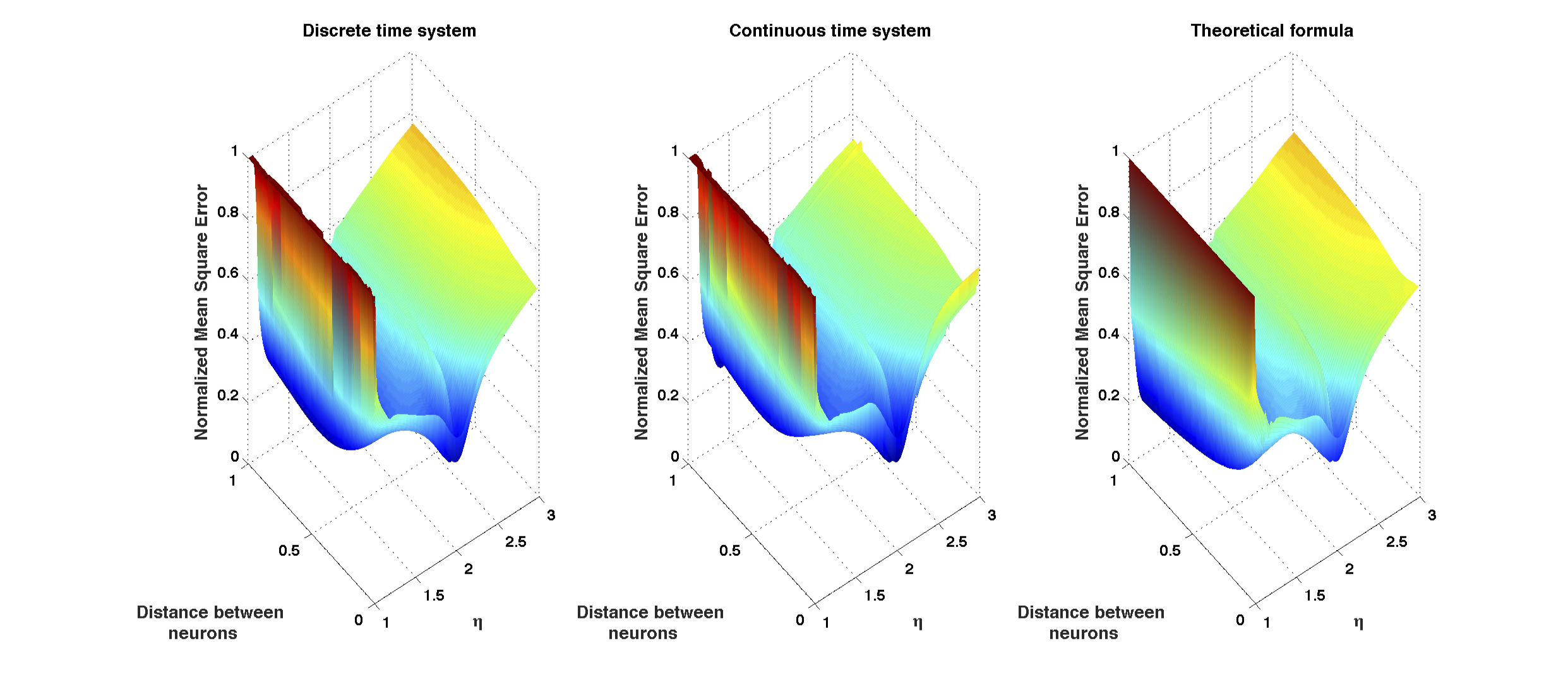
Figure 3: Normalized mean square error surfaces exhibited by an individually operating TDR constructed using a nonlinear Mackey-Glass kernel (2.3) performing a quadratic 3-lags memory task on a 3-dimensional independent mean zero input signal with covariance matrix $\Sigma_{z}$ given by ${\rm vech}(\Sigma_{z})=(0.0016,0.0012,0.0008,0.0017,0.0002,0.0018)$. In these figures the input gain $\gamma=0.6163$ is kept constant. The values of the input mask $C\in\mathbb{M}_{20,3}$ are chosen randomly using a uniform distribution in the interval $\left[-1;1\right]$. The left and middle panels show the error surfaces exhibited by the discrete and continuous time reservoirs computed via Monte Carlo simulations. The right panel shows the error produced by the reservoir model and computed evaluating the explicit capacity formula that can be written down in that case.

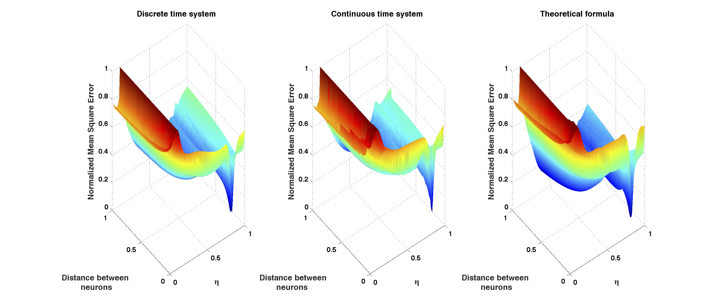
Figure 4: Normalized mean square error surfaces exhibited by an individually operating TDR constructed using a nonlinear Ikeda kernel (2.4) performing a quadratic 3-lags memory task on a 3-dimensional independent mean zero input signal with covariance matrix $\Sigma_{z}$ given by ${\rm vech}(\Sigma_{z})=(0.005,0.0046,0.0041,0.0042,0.0037,0.004)$. In these figures the input gain $\gamma=0.3724$ and the phase shift $\phi=0.7356$ are kept constant. The values of the input mask $C\in\mathbb{M}_{20,3}$ are chosen randomly using a uniform distribution on the interval $\left[-1,1\right]$. The left and middle panels show the error surfaces exhibited by the discrete and continuous time reservoirs computed via Monte Carlo simulations. The right panel shows the error produced by the reservoir model and computed evaluating the explicit capacity formula that can be written down in that case.

Robustness properties of the parallel reservoir architecture.

We now study using the parallel reservoir model introduced in Section 3.2 the robustness properties of the parallel architecture with respect to parameter choice and misspecification task.

(i) Parallel TDR configurations and robustness with respect to the choice of reservoir parameters. An interesting feature of parallel TDR architectures that was observed in [Grig 14] is that optimal performance has a reduced sensitivity with respect to the choice of reservoir parameters when compared to that of individually operating reservoirs. In order to provide additional evidence of this fact, we have constructed parallel pools of 2, 5, 10, and 20 parallel Mackey-Glass-based TDRs and we present to them a nine-lag quadratic memory task is $y(t)=\sum^{9}_{i=0}z(t-i)^{2}$ that, in the terminology introduced in Section 3.3 corresponds to the quadratic task characterized by the vector $Q=\left({\rm vec}(\mathbb{I}_{10})\right)^{\top}D_{10}$, with $D_{10}$ the duplication matrix in dimension ten. For each of these parallel TDR architectures, as well as for an individually operating TDR, we will vary the number of the constituting neurons from 20 to 100. For each of these resulting configurations we randomly draw 1000 sets of input masks with entries uniformly distributed in the interval $[-3,3]$ and reservoir parameters and distance between neurons $d$, also uniformly distributed in the intervals $\eta\in\left[1,3\right]$, $\gamma\in[-3,3]$, and $d\in(0,1)$.

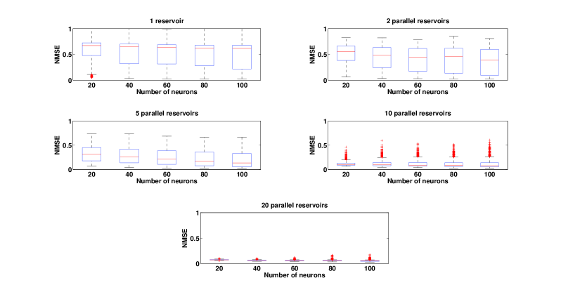
Figure 5: Performance distributions of parallel arrays of Mackey-Glass-based TDRs in a 9-lags quadratic memory task when the kernel parameters and the input mask are varied randomly.

Figure 5 provides the box plots corresponding to the distributions of normalized mean squared errors obtained with each configuration by making the input masks and reservoir parameter values randomly vary, all of them computed using the capacity formulas associated to the parallel reservoir model (3.35). This figure provides striking evidence of the facts that first, the parallel architecture performs on average better and second, that this performance is not sensitive to the choice of reservoir parameters and input mask.

(ii) Parallel TDR configurations and robustness with respect to memory task misspecification. The goal of the next experience is to see how, given a specific memory task and given a parallel array of TDRs or an individually operating one that have been optimized for that particular task, the performance of the different configurations degrades when the task is modified but not the reservoir parameters. We use again parallel pools of 1, 2, 5, 10, and 20 Mackey-Glass-based TDRs with neurons ranging from 10 to 100. For each of those configurations, we choose parameters that optimize their performance with respect to the 3-lag quadratic memory task specified by the matrix $Q=\left({\rm vec}(\mathbb{I}_{4})\right)^{\top}D_{4}$ and with respect to a one-dimensional independent input signal with mean zero and variance $0.0001$. Once the optimal parameters for each configuration have been found using the nonlinear capacity function based on the reservoir model (3.35), we fix them we subsequently expose the corresponding reservoirs to different randomly specified memory tasks of a different specification, namely, 1000 different 9-lag quadratic tasks of the form $Q=\left({\rm vec}(Q^{\ast}_{10})\right)^{\top}D_{10}$, where $Q^{\ast}\in\mathbb{M}_{10}$ is a randomly generated diagonal matrix with entries drawn from the uniform distribution on the interval $[-10;10]$. Figure 6 contains the box plots corresponding to the performance distributions of the different configurations. In this case, parallel architectures offer an improvement on performance and robustness when compared to the single reservoir design. The most visible improvement is obtained in this case when using a parallel pool of two reservoirs.

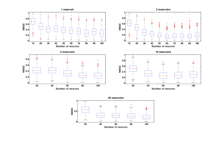
Figure 6: Robustness of the performance of parallel arrays of Mackey-Glass kernel based TDRs with respect to task misspecification. The box plots report the distribution of normalized mean square errors committed in the execution of 1000 randomly generated 9-lag diagonal quadratic memory tasks by different TDR configurations that had been initially optimized for a 3-lag quadratic memory task.

References

• [Appe 11] L. Appeltant, M. C. Soriano, G. Van der Sande, J. Danckaert, S. Massar, J. Dambre, B. Schrauwen, C. R. Mirasso, and I. Fischer. “Information processing using a single dynamical node as complex system”. Nature Communications, Vol. 2, p. 468, Jan. 2011.
• [Atiy 00] A. F. Atiya and A. G. Parlos. “New results on recurrent network training: unifying the algorithms and accelerating convergence”. IEEE transactions on neural networks / a publication of the IEEE Neural Networks Council, Vol. 11, No. 3, pp. 697–709, Jan. 2000.
• [Brun 13] D. Brunner, M. C. Soriano, C. R. Mirasso, and I. Fischer. “Parallel photonic information processing at gigabyte per second data rates using transient states”. Nature Communications, Vol. 4, No. 1364, 2013.
• [Croo 07] N. Crook. “Nonlinear transient computation”. Neurocomputing, Vol. 70, pp. 1167–1176, 2007.
• [Crut 10] J. P. Crutchfield, W. L. Ditto, and S. Sinha. “Introduction to focus issue: intrinsic and designed computation: information processing in dynamical systems-beyond the digital hegemony”. Chaos (Woodbury, N.Y.), Vol. 20, No. 3, p. 037101, Sep. 2010.
• [Grig 14] L. Grigoryeva, J. Henriques, L. Larger, and J.-P. Ortega. “Stochastic time series forecasting using time-delay reservoir computers: performance and universality”. Neural Networks, Vol. 55, pp. 59–71, 2014.
• [Grig 15a] L. Grigoryeva, J. Henriques, L. Larger, and J.-P. Ortega. “Optimal nonlinear information processing capacity in delay-based reservoir computers”. Scientific Reports, Vol. 5, No. 12858, pp. 1–11, 2015.
• [Grig 15b] L. Grigoryeva and J.-P. Ortega. “Ridge regularized multidimensional regressions: error evaluation with estimated regression parameters”. Preprint, 2015.
• [Gupt 00] A. Gupta and D. Nagar. Matrix Variate Distributions. Chapman and Hall/CRC, 2000.
• [Holm 88] B. Holmquist. “Moments and cumulants of the multivariate normal distribution”. Stochastic Analysis and Applications, Vol. 6, No. 3, pp. 273–278, Jan. 1988.
• [Iked 79] K. Ikeda. “Multiple-valued stationary state and its instability of the transmitted light by a ring cavity system”. Optics Communications, Vol. 30, No. 2, pp. 257–261, Aug. 1979.
• [Jaeg 01] H. Jaeger. “The ’echo state’ approach to analysing and training recurrent neural networks”. Tech. Rep., German National Research Center for Information Technology, 2001.
• [Jaeg 04] H. Jaeger and H. Haas. “Harnessing Nonlinearity: Predicting Chaotic Systems and Saving Energy in Wireless Communication”. Science, Vol. 304, No. 5667, pp. 78–80, 2004.
• [Jaeg 07] H. Jaeger, M. Lukoševičius, D. Popovici, and U. Siewert. “Optimization and applications of echo state networks with leaky-integrator neurons”. Neural Networks, Vol. 20, No. 3, pp. 335–352, 2007.
• [Larg 12] L. Larger, M. C. Soriano, D. Brunner, L. Appeltant, J. M. Gutierrez, L. Pesquera, C. R. Mirasso, and I. Fischer. “Photonic information processing beyond Turing: an optoelectronic implementation of reservoir computing”. Optics Express, Vol. 20, No. 3, p. 3241, Jan. 2012.
• [Luko 09] M. Lukoševičius and H. Jaeger. “Reservoir computing approaches to recurrent neural network training”. Computer Science Review, Vol. 3, No. 3, pp. 127–149, 2009.
• [Lutk 05] H. Lütkepohl. New Introduction to Multiple Time Series Analysis. Springer-Verlag, Berlin, 2005.
• [Maas 02] W. Maass, T. Natschläger, and H. Markram. “Real-time computing without stable states: a new framework for neural computation based on perturbations”. Neural Computation, Vol. 14, pp. 2531–2560, 2002.
• [Maas 11] W. Maass. “Liquid state machines: motivation, theory, and applications”. In: S. S. Barry Cooper and A. Sorbi, Eds., Computability In Context: Computation and Logic in the Real World, Chap. 8, pp. 275–296, 2011.
• [Mack 77] M. C. Mackey and L. Glass. “Oscillation and chaos in physiological control systems”. Science, Vol. 197, pp. 287–289, 1977.
• [Meye 00] C. Meyer. Matrix Analysis and Applied Linear Algebra Book and Solutions Manual. Society for Industrial and Applied Mathematics, 2000.
• [Orti 12] S. Ortin, L. Pesquera, and J. M. Gutiérrez. “Memory and nonlinear mapping in reservoir computing with two uncoupled nonlinear delay nodes”. In: Proceedings of the European Conference on Complex Systems, pp. 895–899, 2012.
• [Paqu 12] Y. Paquot, F. Duport, A. Smerieri, J. Dambre, B. Schrauwen, M. Haelterman, and S. Massar. “Optoelectronic reservoir computing”. Scientific reports, Vol. 2, p. 287, Jan. 2012.
• [Roda 11] A. Rodan and P. Tino. “Minimum complexity echo state network.”. IEEE transactions on neural networks / a publication of the IEEE Neural Networks Council, Vol. 22, No. 1, pp. 131–44, Jan. 2011.
• [Tria 03] K. Triantafyllopoulos. “On the central moments of the multidimensional Gaussian distribution”. The Mathematical Scientist, Vol. 28, pp. 125–128, 2003.
• [Vers 07] D. Verstraeten, B. Schrauwen, M. D Haene, and D. Stroobandt. “An experimental unification of reservoir computing methods”. Neural Networks, Vol. 20, pp. 391–403, 2007.