CosmoSpec: Fast and detailed computation of the cosmological recombination radiation from hydrogen and helium

Abstract

We present the first fast and detailed computation of the cosmological recombination radiation released during the hydrogen (redshift $z\simeq 1300$) and helium ($z\simeq 2500$ and $z\simeq 6000$) recombination epochs, introducing the code CosmoSpec. Our computations include important radiative transfer effects, $500$-shell bound-bound and free-bound emission for all three species, the effects of electron scattering and free-free absorption as well as interspecies ($\text{He\,{ii}}\rightarrow\text{He\,{i}}\rightarrow\text{H\,{i}}$) photon feedback. The latter effect modifies the shape and amplitude of the recombination radiation and CosmoSpec improves significantly over previous treatments of it. Utilizing effective multilevel atom and conductance approaches, one calculation takes only $\simeq 15$ seconds on a standard laptop as opposed to days for previous computations. This is an important step towards detailed forecasts and feasibility studies considering the detection of the cosmological recombination lines and what one may hope to learn from the $\simeq 6.1$ photons emitted per hydrogen atom in the three recombination eras. We briefly illustrate some of the parameter dependencies and discuss remaining uncertainties in particular related to collisional processes and the neutral helium atom model.

1 Introduction

The energy spectrum of the cosmic microwave background (CMB) allows probing the thermal history of the Universe (Zeldovich & Sunyaev, 1969; Sunyaev & Zeldovich, 1970; Burigana et al., 1991; Hu & Silk, 1993), with several interesting standard and non-standard signals awaiting us (for overview see Chluba & Sunyaev, 2012; Sunyaev & Khatri, 2013; Tashiro, 2014). One of the guaranteed signals is imprinted by the cosmological recombination process (Zeldovich et al., 1968; Peebles, 1968; Dubrovich, 1975) at redshifts $z\simeq 10^{3}-10^{4}$. It appears as a spectral distortion of the CMB that today is visible at frequencies $\nu\simeq 0.1\,{\rm GHz}-2\,{\rm THz}$ (Sunyaev & Chluba, 2009). The cosmological recombination radiation (CRR) constitutes a fundamental signal from the early Universe that can provide an alternative way to measure some of the key cosmological parameters (e.g., Chluba & Sunyaev, 2008b; Sunyaev & Chluba, 2009) and allow testing the physics of the cosmological recombination process. As challenging as the detection of the CRR may be (Sathyanarayana Rao et al., 2015; Desjacques et al., 2015; Balashev et al., 2015), it is a highly desirable target for future CMB studies (Silk & Chluba, 2014), and may be possible with an improved version of PIXIE (Kogut et al., 2011) or PRISM (André et al., 2014).

Nowadays, the detailed recombination history (the free electron fraction as a function of redshift) can be computed with $\lesssim 0.1\%$ precision around decoupling ($z\simeq 10^{3}$) using CosmoRec (Chluba & Thomas, 2011) and HyRec (Ali-Haïmoud & Hirata, 2011). This precision is required to ensure that our interpretation of CMB data from Planck gives unbiased results in particular for the spectral index of primordial fluctuation and the baryon density (Rubiño-Martín et al., 2010; Shaw & Chluba, 2011; Planck Collaboration et al., 2015a).

While in terms of standard (atomic) physics the recombination history is expected to be well understood, non-standard process, for instance, due to decaying or annihilating particles (e.g., Peebles et al., 2000; Chen & Kamionkowski, 2004; Padmanabhan & Finkbeiner, 2005; Galli et al., 2009a; Hütsi et al., 2009; Slatyer et al., 2009; Giesen et al., 2012) or variations of fundamental constants (e.g., Kaplinghat et al., 1999; Battye et al., 2001; Rocha et al., 2003; Scóccola et al., 2009; Galli et al., 2009b) can modify the ionization history. These scenarios can be constrained with CMB temperature and polarization data (Planck Collaboration et al., 2015a, b). It is, however, hard to discern between different sources of changes to the recombination history. Similarly, when allowing standard parameters such as the helium mass fraction, $Y_{\rm p}$, and effective number of neutrino species, $N_{\rm eff}$, to vary simultaneously, large degeneracies remain (Planck Collaboration et al., 2015a). In all these cases, the CRR is expected to provide extra pieces of the puzzle, which will help to break degeneracies and directly probe the recombination dynamics (Chluba & Sunyaev, 2008b; Sunyaev & Chluba, 2009; Chluba, 2010). In addition, the reaction of the plasma in the pre-recombination era can give hints about early energy release (Lyubarsky & Sunyaev, 1983; Chluba & Sunyaev, 2009b). It is thus important to understand how the CRR depends on different assumptions, and a detailed computation of the signals for the standard scenario is the first step.

Several calculations of the CRR have been carried out in the past using different methods and approximations (e.g., Dubrovich, 1975; Rybicki & dell’Antonio, 1993; Dubrovich & Stolyarov, 1995, 1997; Burgin, 2003; Kholupenko et al., 2005; Wong et al., 2006; Rubiño-Martín et al., 2006; Chluba et al., 2007). In Sect. 3, we dwell deeper into the details, but the biggest problem is that these calculations either included a small number of atomic levels, neglected physical processes and/or took prohibitively long to allow detailed computations for many cosmologies. The situation was very similar back in the early days of CMB cosmology when slow Boltzmann codes (Ma & Bertschinger, 1995; Hu et al., 1995) were used for computations of the CMB power spectra.

In this work, we take the next step for computations of the CRR, developing the software package CosmoSpec, which allows fast and precise computation of the CRR for a wide range of cosmological models including all important physical processes. The computational method is based on a combination of the effective multilevel atom (Ali-Haïmoud & Hirata, 2010) and effective conductance approach (Ali-Haïmoud, 2013), which we briefly review in Sect. 3. These approaches are similar in spirit to the line-of-sight approach for CMB anisotropies (Seljak & Zaldarriaga, 1996) used in modern Boltzmann codes CMBfast, CAMB (Lewis et al., 2000) or CLASS (Lesgourgues, 2011), in the sense that they rely on a factorization of the problem into a slow but cosmology-independent part and a fast, cosmology-dependent part.

With CosmoSpec the calculation of the CRR for one cosmology can be performed in $\simeq 15$ seconds on a standard laptop, a performance that opens the path for detailed parameter explorations and experimental forecasts, applications we leave to future work. We discuss the importance of different physical processes, such as interspecies feedback, collisions and uncertainties in the atomic model for neutral helium (Sect. 4). Overall, CosmoSpec in its current state should be accurate at the level of a few percent for the standard recombination scenario, mainly due to uncertainties of the neutral helium atom model.

2 Atomic models

For the computations presented here, we adopt atomic models for hydrogen and helium closely following Rubiño-Martín et al. (2006); Chluba et al. (2007) and Rubiño-Martín et al. (2008). Below we briefly summaries the main aspects of these models, but refer to the above references for details.

2.1 Hydrogen and hydrogenic helium

Level energies, electric dipole transitions rates, and photoionization cross sections for hydrogenic ions can be computed analytically using the expressions of Karzas & Latter (1961) and the recursion method of Storey & Hummer (1991) (see also Hey, 2006). Corrections due to the Lamb shift are neglected. We also omit H i and He ii quadrupole transitions, which coincide with the dipole transition frequencies and have been shown to cause a negligible effect on the recombination dynamics (Grin & Hirata, 2010; Chluba et al., 2012) and thus should not change the H i and He ii recombination radiation significantly.

We use the hydrogen radiative transfer module of CosmoRec (Chluba & Thomas, 2011), resolving the 2s, 2p, 3s, 3p and 3d states. This includes, Lyman-$\alpha$ and $\beta$ resonance scattering as well as two-photon emission and Raman scattering events. Electron scattering is added using a Fokker-Planck approach (Hirata & Forbes, 2009; Chluba & Sunyaev, 2009a) to improve the stability of the transfer calculation, but we neglect modifications caused by the detailed shape of the scattering kernel (Ali-Haïmoud et al., 2010). The results of the transfer calculation are used to obtain the high-frequency distortion caused by hydrogen. The H i 2s-1s two-photon decay rate is set to $A^{\rm HI}_{\rm 2s1s}=8.2206\,\sec^{-1}$ (Labzowsky et al., 2005).

For hydrogenic helium, we approximate the 2s-1s two-photon profile using the expression of Nussbaumer & Schmutz (1984):

$$\phi(y)=C\left[w(1-4^{\gamma}\,w^{\gamma})+\alpha\,w^{\beta+\gamma}\,4^{\gamma}\right]\,,$$ (1)

where $y=\nu/\nu_{\rm 2s1s}$, $w=y[1-y]$, $C=12.278$, $\alpha=0.88$, $\beta=1.53$ and $\gamma=0.8$. The two-photon profile is normalized as $\int\phi(y){\,\rm d}y=2$, since two photons are emitted per transition. We set the He ii two-photon decay rate to $A^{\rm HeII}_{\rm 2s1s}=526.57\,\sec^{-1}$. For He ii, we use an effective multilevel atom approach with Sobolev escape probability formalism. No separate radiative transfer calculation is performed.

2.2 Neutral helium

The atomic model for helium significantly more complex than the one of hydrogenic ions and, more importantly, more uncertain. The main complication is due to the fact that the neutral helium atom is a three particle system (nucleus + two electrons), so that no closed analytic solutions exist.

2.2.1 Energies and transitions

For the energies and transitions rates among the singlet and triplet levels with principal quantum numbers $n\leq 10$ we use the multiplet tables from Drake & Morton (2007). These tables have a few gaps (e.g., for level $\{n,l,s,j\}=\{10,7,0,7\}$), which we fill with hydrogenic values (see Appendix A for details). To obtain the energies of levels with $10<n\leq 30$ and $l\leq 6$ we use the quantum defect method (e.g., see Drake, 2006), while for all other levels we use the simple hydrogenic approximation for the level energy, $E_{n}\approx-E_{\rm He}/n^{2}$, where $E_{\rm He}=hc\,R_{\infty}/(1+m_{\rm e}/M_{\rm He})$, $m_{\rm e}/M_{\rm He}\approx 1.3709\times 10^{-4}$ is the electron to helium mass ratio and $R_{\infty}\approx 1.0974\times 10^{7}\,{\rm m^{-1}}$ is the Rydberg constant. For levels with $n>10$, we generally do not include $J$-resolved levels. For transitions between levels with $n>10$, we use hydrogenic transitions rates, rescaled by the second power of the transitions frequency. This approximation is rather crude for transitions involving low-$\ell$ states (i.e., $n$S through $n$D) as illustrated below (Sect. 4.6). No singlet-triplet transitions are allowed among excited states with $n>10$. For transitions from excited levels to $n^{\prime}\leq 10$, we use hydrogenic values following Rubiño-Martín et al. (2008), which have the correct average property (Appendix A). We also include a few extra transitions (see Chluba & Sunyaev, 2010; Chluba et al., 2012, for more details), for example, singlet-triplet transitions (Switzer & Hirata, 2008a) and additional He i quadrupole lines (Cann & Thakkar, 2002) to the ground-state. The radiative transfer problem for He i is solved using CosmoRec (for details see, Chluba et al., 2012).

We approximate the He i ${2^{1}{\rm S}_{0}}-{1^{1}{\rm S}_{0}}$ two-photon profile using (Drake, 1986; Switzer & Hirata, 2008a):

$$\phi(y)=C\,\frac{w^{3}}{(w+\delta)^{2}}\,\left[\alpha-\beta w+\gamma w^{2}\right]\,,$$ (2)

where $y=\nu/\nu_{{2^{1}{\rm S}_{0}}-{1^{1}{\rm S}_{0}}}$, $w=y[1-y]$, $C=19.604$, $\alpha=1.742$, $\beta=7.2$, $\gamma=12.8$ and $\delta=0.03$. Again, the two-photon profile is normalized as $\int\phi(y){\,\rm d}y=2$. We use $A^{\rm HeI}_{\rm 2s1s}=51.3\,\sec^{-1}$ (Drake et al., 1969) for the total two-photon decay rate. The effect of other two-photon and Raman processes (Hirata & Switzer, 2008) on the recombination dynamics and shape of the high-frequency distortion are neglected. We also neglect corrections caused by the detailed photon redistribution kernel of electron and line scattering (Switzer & Hirata, 2008b; Chluba et al., 2012).

2.2.2 Photoionization cross section

As pointed out previously (e.g., Rubiño-Martín et al., 2008; Chluba & Sunyaev, 2010; Glover et al., 2014), for the CRR one of the biggest uncertainty in the neutral helium model is due to the lack of data for the photoionization cross sections. For levels with $n\leq 10$ and $l\leq 3$, we use a combination of the sparse TopBase data (Cunto et al., 1993) and pre-calculated recombination rates from Smits (1996). For all other levels, we use hydrogenic approximations for the photoionization cross section, following Rubiño-Martín et al. (2008). The $J$-resolved photoionization cross section is simply set to $\sigma^{\rm He}_{nLJ}(\nu)\approx\sigma^{\rm H}_{nL}(\nu_{i\rm c}^{\rm H}\,\nu/\nu_{i\rm c}^{\rm He})$ using the ionization threshold frequencies for hydrogen and helium, $\nu_{i\rm c}^{\rm H}$ and $\nu_{i\rm c}^{\rm He}$. For the recombination rate this implies a rescaling by $\simeq(\nu_{i\rm c}^{\rm He}/\nu_{i\rm c}^{\rm H})^{3}$. This approximation is obtained by assuming that the $J$-averaged cross section is equal to the hydrogenic one and using the fact that $J$-resolved cross sections are all equal, up to small corrections due to the fine splitting of $J$-sub-levels (see Appendix A.1). It also neglects corrections to the shape of the cross section, in particular due to auto-ionization resonances, which are important for the low-$\ell$ states. This leads to uncertainties in the shape of the free-bound spectrum, as we briefly discuss in Sect. 4.6.

3 Computational method

3.1 Effective multilevel atom and conductance methods

One of the biggest challenges for detailed and fast computation of the cosmological recombination history and radiation is that in explicit multilevel approaches (e.g., Seager et al., 2000; Chluba et al., 2007) the populations of many levels ($\simeq n_{\rm max}^{2}/2$ for hydrogen) have to be followed to determine their departures from full equilibrium. For 500-shell calculations of hydrogen this includes some $\simeq 10^{5}$ levels, which makes the computations very time-consuming (e.g., Rubiño-Martín et al., 2006; Grin & Hirata, 2010; Chluba et al., 2010). However, the effect of excited states can be integrated out using the effective multilevel atom method for the recombination history (Ali-Haïmoud & Hirata, 2010) and the effective conductance method for the recombination radiation (Ali-Haïmoud, 2013).

The effective multilevel atom is an exact generalization of the effective three-level atom model (Peebles, 1968; Zeldovich et al., 1968). In this approach, the case-B recombination coefficient is replaced by effective recombination coefficients $\mathcal{A}_{i}(T_{\rm e},T_{\gamma})$ to a few low-lying excited states. These coefficients account for stimulated recombinations and the finite probability of photoionization as a captured electron cascades down to the lowest excited states. In the absence of collisional transitions, they are functions of the electron ($T_{\rm e}$) and photon ($T_{\gamma}$) temperatures only. These coefficients are supplemented by effective photoionization rates $\mathcal{B}_{i}(T_{\gamma})$ and effective transition rates between the low-lying excited states, $\mathcal{R}_{i\rightarrow j}(T_{\gamma})$. The calculation of the effective rates to high accuracy is computationally demanding, as it requires solving large linear algebra problems. However, it has to be done only once. For any cosmology, the recombination history can then be computed very efficiently by solving an effective few-level system, and interpolating the effective rates whenever they are needed. The effective multilevel approach is the basis for the cosmological recombination codes HyRec (Ali-Haïmoud & Hirata, 2011) and CosmoRec (Chluba & Thomas, 2011) which are now directly used for the analysis of high-precision CMB data from Planck (Planck Collaboration et al., 2015a).

The effective conductance method (Ali-Haïmoud, 2013) allows to factorize the computation of the recombination radiation into a slow, cosmology-independent part, and a fast, cosmology-dependent part. In this approach, the net emissivity (or intensity) in any bound-bound or free-bound transition is rewritten as a sum of temperature-dependent coefficients (effective conductances) times departures from equilibrium of the populations of the lowest-lying excited states (which play the role of tensions). The former are pre-tabulated as a function of transition energy and temperature, while the latter are obtained very efficiently, for any particular cosmology, by solving the effective few-level atom described above.

Here, we extend CosmoRec to allow detailed computation of the $\text{He\,{iii}}\rightarrow\text{He\,{ii}}$ recombination history using an effective multilevel approach. Similarly, we update the effective rate coefficients for neutral helium to include 500 shells. While the effective rates and conductances for neutral helium have to be explicitly computed, those for hydrogenic helium can be obtained from those for hydrogen by simple rescaling which we derive in Appendix B.

3.2 Electron scattering

Line broadening and shifting caused by scattering with free electrons was found to be important for the He ii recombination radiation (Rubiño-Martín et al., 2008). To include these effects we use the improved approximation for the electron scattering Green’s function of the photon occupation number given by Chluba (2015):

$$G(x^{\prime},x,y) =\frac{\exp\left(-\left[\ln(x/x^{\prime})-\alpha\,y+\ln(1+x^{\prime}y)\right]^{2}/4y\,\beta\right)}{\sqrt{4\pi y\,\beta}\,x^{3}}.$$ (3)

Here, $x=h\nu/kT_{\gamma}$ and $y=\int(kT_{\rm e}/m_{\rm e}c^{2})\,\sigma_{\rm T}N_{\rm e}c{\,\rm d}t$ denotes the scattering $y$-parameter. We also introduced $\alpha=[3-2f(x^{\prime})]/\sqrt{1+x^{\prime}y}$ and $\beta=(1+x^{\prime}y[1-f(x^{\prime})])^{-1}$, with $f(x)={{\rm e}^{-x}}(1+x^{2}/2)$, which were obtained by matching the numerical solution. This approximation improves over the classical solution ($\alpha=3$, $\beta=1$ and $\ln(1+x^{\prime}y)\rightarrow 0$) of Zeldovich & Sunyaev (1969) by accounting for the effect of electron recoil at high frequencies and including the blackbody-induced stimulated scattering (Chluba & Sunyaev, 2008a) at low frequencies.

To compute the contribution to frequency bin $x_{j}$ caused by the scattering of photons emitted at frequency $x_{i}$ and redshift $z$, we find

$$\Delta I^{\rm sc}_{j} =\frac{\Delta I_{i}(z)}{2\,x_{i}}\Big{[}{\rm erf}(b_{u})-{\rm erf}(b_{l})\Big{]}{{\rm e}^{-a_{i}+y\,\beta_{i}}}$$

$$\approx\frac{\Delta I_{i}(z)}{x_{i}}\,\frac{{{\rm e}^{-a_{i}+y\,\beta_{i}-b_{j}^{2}}}}{\sqrt{4\pi y\,\beta_{i}}}\,\frac{x_{u}-x_{l}}{x_{j}}.$$ (4)

We integrated across the bin between $x_{l}$ and $x_{u}$ with $x_{j}=(x_{u}+x_{l})/2$. Here, $a_{i}=-\ln x_{i}-\alpha(x_{i})\,y+\ln(1+x_{i}y)$, $b_{k}=(a_{i}-2y\,\beta_{i}+\ln x_{k})/2\sqrt{y\,\beta_{i}}$ and $\Delta I_{i}(z)$ denotes the distortion caused by the process without including electron scattering. The second line in Eq. (3.2) was obtained assuming a narrow bin $x_{u}-x_{l}\ll x_{j}$. The $y$-parameter is computed between the emission redshift $z$ and today using the solution for the electron recombination history of CosmoRec. Around the maximum of emission from He ii ($z\simeq 6000$) we find $y\simeq 10^{-3}$, so that the line broadening reaches $\Delta\nu/\nu\simeq 2\sqrt{y\ln 2}\simeq 5\%$. During neutral helium and hydrogen recombination, electron scattering is much less important and can safely be neglected.

3.3 Free-free absorption

At low frequencies ($\nu\lesssim 0.1-1\,{\rm GHz}$), free-free absorption becomes noticeable (Chluba et al., 2007). So far, this effect was only taken into account for the H i recombination radiation. It is, however, slightly more important for the helium recombination spectra, as we show below (Sect. 4). To include this process, we modify the emission in each frequency bin $x_{i}$ and redshift $z$ by

$$\Delta I^{\rm ff}_{i} =\Delta I_{i}(z)\,{{\rm e}^{-\tau_{\rm ff}(x_{i},z)}},$$ (5)

where the free-free absorption optical depth is roughly given by, $\tau_{\rm ff}(x,z)\approx F(z)\ln(2.25/x)/x^{2}$, and $F(z)$ is a single redshift-dependent function. This function can be computed using approximations for the free-free Gaunt factors (e.g., Itoh et al., 2000; Draine, 2011). The efficiency of free-free absorption drops exponentially around hydrogen recombination ($z\simeq 10^{3}$), but earlier it is important at low frequencies. More details can be found in Chluba (2015).

3.4 Feedback due to helium photons

The feedback physics is simple: energetic photons, emitted during the two recombination phases of helium, can ionize and excite the next-lying species at a later time. Specifically, He ii photons feedback onto He i and H i atoms, and He i photons feedback onto H i atoms. These ionizations and excitations typically take place earlier than the epoch of recombination of the lower-lying species, and are instantaneously compensated by rapid recombinations and decays, generating a pre-recombination radiation from the species that is subjected to feedback. In the case of $\text{He\,{ii}}\rightarrow\text{He\,{i}}$ feedback, the pre-recombination emission from He i can itself feedback onto hydrogen (Chluba & Sunyaev, 2010; Chluba et al., 2012).

Part of the $\text{He\,{i}}\rightarrow\text{H\,{i}}$ feedback is already included in previous calculation for the hydrogen recombination radiation (Rubiño-Martín et al., 2008). However, as shown in Chluba & Sunyaev (2010), changes in the recombination dynamics due to He ii feedback cause significant additional modifications of the CRR. In Chluba & Sunyaev (2010), these corrections were only included for 20-shell calculations, which here we extend to 500 shells. Furthermore, changes to the detailed time-dependence of the feedback process because of radiative transfer effects (e.g., broadening by electrons scattering of the He ii Lyman-$\alpha$ line) were neglected. These effects can be readily included in our new computation. For this we modify the radiative transfer calculation of neutral helium, including the emission of photons in the He ii Lyman-$\alpha$ line and 2s-1s two-photon continuum. These photons then redshift and feedback on neutral helium and hydrogen in their respective pre-recombination eras causing the production of extra photons. Our treatment automatically includes corrections due to line broadening by electron and resonance scattering. The results of these calculations will be presented in Sect. 4.2.

3.5 Collisional transitions

Collisional processes can modify the atomic level populations of the highly excited states. This affects the recombination dynamics and the low-frequency emission, originating from transitions involving highly excited states ($n\gtrsim 30-50$). For hydrogen, collisional processes were found to have a minor effect for both aspects (Chluba et al., 2007, 2010), however, because collisions become more important at higher densities, for helium this may no longer be true, in particular for the pre-recombination emission.

3.5.1 Angular-momentum-changing collisions

Angular-momentum-changing collisions are the most important for the recombination history and the CRR. To estimate the effect of $\ell$-changing collision among energetically degenerate levels (modeling them with hydrogenic wave functions), we use the classical approximation of Vrinceanu et al. (2012), which we extend to general ion and nucleus charge:

$$C_{n\ell\rightarrow n\ell^{\prime}} \approx 2.6\times 10^{-5}\sqrt{\frac{M}{m_{\rm e}}}\,\frac{(Z^{2}_{\rm ion}/Z^{2}_{\rm nuc})\,N_{\rm ion}}{\sqrt{T_{\rm e}/{\rm K}}}$$

$$\qquad\times\frac{n^{2}\left[n^{2}(\ell+\ell^{\prime})-\ell^{2}_{<}(\ell+\ell^{\prime}+2|\Delta\ell|)\right]}{(2\ell+1)\,|\Delta\ell|^{3}}\,{\rm cm}^{3}\,{\rm s}^{-1},$$ (6)

where $N_{\rm ion}$ is the number density of the projectiles, $\ell_{<}=\min(\ell,\ell^{\prime})$, $M$ is the reduced mass of the ion-target system; $Z_{\rm ion}$ the charge of the projectile and $Z_{\rm nuc}$ that of the nucleus ($Z_{\rm nuc}=1$ for hydrogen and neutral helium, and 2 for singly-ionized helium). We give a simple derivation of Eq. (3.5.1) in Appendix C, valid for $\ell,\ell^{\prime},n\gg 1$. We also argue that the underlying assumption of a straight-line trajectory for the colliding ion is very accurate at the relevant temperatures, even when the target is charged as is the case for singly-ionized helium. For $\ell$-mixing, proton and $\alpha$-particle collisions are more important than electron collisions (which we neglect).

Equation (3.5.1) automatically obeys detailed balance and provides an estimate for transition with $|\Delta\ell|>1$, in very good agreement with the full quantum calculation (Vrinceanu et al., 2012). It can be applied for all three species, since $\ell$-changing collisions are only important for highly-excited states ($n\gtrsim 30-50$), which even for neutral helium are close to hydrogenic. It does, however, omit the possibility of collision-induced singlet-triplet state mixing.

For $\Delta\ell=\pm 1$, the quantum-mechanical transition probability scales as $1/b^{2}$ for large impact parameters, while the classical transition probability used to obtain Eq. (3.5.1) vanishes beyond a maximum impact parameter (see Fig. 1 in Vrinceanu et al., 2012, as well as our Appendix C). To obtain a finite collision rate with the full quantum description, one therefore needs to cut off the integration at some maximum impact parameter (Vrinceanu & Flannery, 2001). Since the divergence is only logarithmic, the choice of the cutoff is not critical and the result is found to be well approximated by Eq. (3.5.1) (Sadeghpour, 2015, private communication). It is lower by a factor of a few than the previous estimate of Pengelly & Seaton (1964), whose Born approximation calculation required a regularization at both large and small impact parameters.

3.5.2 Collisional excitations and de-excitations

For collisional de-excitation rates of ions or atoms by electron impact we use the expression of van Regemorter (1962):

$$C_{i\rightarrow j}\approx 20.6\,N_{\rm e}\,\lambda_{ij}^{3}\,\frac{A_{i\rightarrow j}}{\sqrt{T_{\rm e}/{\rm K}}}\,P(h\nu_{ij}/kT_{\rm e}),$$ (7)

where $i$ and $j$ are the the upper and lower levels, respectively, $\lambda_{ij}=c/\nu_{ij}$ is the transition wavelength, $A_{i\rightarrow j}$ is the Einstein-A coefficient of the transition and the function $P(y)$ depends on whether the target is neutral or positive. At high temperatures, it scales as $P(y)\approx-0.159-0.276\ln y$ in both cases. The collisional excitation rate is obtained by detailed balance: $C_{j\rightarrow i}=(g_{i}/g_{j}){{\rm e}^{-h\nu_{ij}/kT_{\rm e}}}C_{i\rightarrow j}$.

3.5.3 Collisional ionizations and three-body recombinations

For the collisional ionization rate by electron impact, we use the simple expression (see, Mihalas, 1978; Mashonkina, 1996):

$$C_{i\rightarrow\rm c}\approx 1.55\times 10^{13}\,\bar{g}\,N_{\rm e}\,\frac{\sigma_{i\rightarrow\rm c}(\nu_{i\rm c})}{\sqrt{T_{\rm e}/{\rm K}}}\,\frac{{{\rm e}^{-h\nu_{i\rm c}/kT_{\rm e}}}}{h\nu_{i\rm c}/kT_{\rm e}}\,{\rm cm}\,{\rm s}^{-1},$$ (8)

where $\sigma_{i\rightarrow\rm c}(\nu_{ic})$ is the photoionization cross section at threshold, $\bar{g}=0.2$ for hydrogen and neutral helium and $\bar{g}=0.3$ for hydrogenic helium. The collisional recombination coefficient follows from detailed balance.

The rate coefficients for collisional ionization and excitation are uncertain. However, they turn out to have a very small effect on the CRR, as we shall discuss in Sect. 4.5.

3.5.4 Inclusion in the effective rates and conductances

One can simply generalize the effective multilevel and effective conductance methods to account for collisional transitions. The effective rates and conductances are then not only functions of temperature, but also the collider densities, $N_{\rm coll}=\{N_{\rm e},N_{\rm p},N_{\rm He}^{+},N_{\rm He}^{++}\}$. In principle this adds more dimensions over which to tabulate the effective rates. However, since the cosmological parameters are known to percent accuracy, so is the evolution of the main collider densities as a function of $T_{\gamma}$. It would therefore probably be enough to compute the values and first few derivatives of the effective rates with respect to the densities around their best-fit values $N_{\rm coll}^{0}(T_{\gamma})$. However, given that the uncertainty of the collisional rates is still large compared to the precision of the standard cosmological parameters, in this paper we simply compute the effective rates and conductances at the best-fit collider densities $N_{\rm coll}^{0}(T_{\gamma})$.

4 Results

After obtaining all the effective rates and conductances, both the computation of the recombination history and recombination radiation boils down to solving a moderate system of coupled ordinary differential and partial differential equations and numerical integrals. This accelerates the calculation by a large amount, making it feasible to perform one full calculation within $\simeq 15$ seconds on a standard laptop. Here, we illustrate the results for the recombination radiation, highlighting some of the new aspects and comparison with previous computations.

4.1 Comparison with previous computations

To validate our new treatment, we first compare our results with previous calculations of the recombination radiation. For hydrogen, detailed multilevel recombination computations for the bound-bound emission, including up to 350 $\ell$-resolved shells ($\simeq 61,000$ individual levels), were presented in Chluba et al. (2010). These calculations also included the effect of H i Lyman-continuum absorption during the He i recombination era (Kholupenko et al., 2007; Switzer & Hirata, 2008a), an effect that leads to pre-recombination emission from hydrogen (Rubiño-Martín et al., 2008; Chluba & Sunyaev, 2010). In Ali-Haïmoud (2013), the effective conductance method was used to compute the recombination radiation from hydrogen for 500 $\ell$-resolved shells, also including the free-bound radiation, which previously was only available for $100$-shell hydrogen calculations (Chluba & Sunyaev, 2006a). Comparing with the results from our new computation for similar settings (in terms of the included physics and atomic model), we find excellent agreement at the level of $\simeq 0.1\%-1\%$ with these previous computations. While this validates our implementation, here we add corrections due to feedback from He ii photons, which increases the emission caused by hydrogen and neutral helium (see Sect. 4.2).

For singly-ionized helium, we compare with the multilevel computations presented in Rubiño-Martín et al. (2008) for 100 shells. Only results for the bound-bound radiation were previously presented, for which we find excellent agreement both with and without electron scattering included. For the neutral helium recombination emission only the bound-bound emission for up to 30 shells was previously considered (Rubiño-Martín et al., 2008). Extending the multilevel code of Chluba et al. (2010) to include more levels for neutral helium, we confirmed the results of our conductance method. For the bound-bound radiation, at low frequencies ($\nu\lesssim 20\,{\rm GHz}$) our results deviate from the spectrum presented in Rubiño-Martín et al. (2008). We attribute these differences to variations in the atomic model of neutral helium (in particular the recombination rates to excited states), however, the main high-frequency features agree well with our improved calculations. Here we also add the two free-bound contributions from both helium ions, which have not been obtained before.

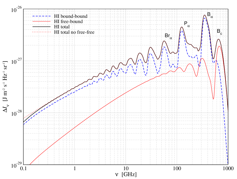
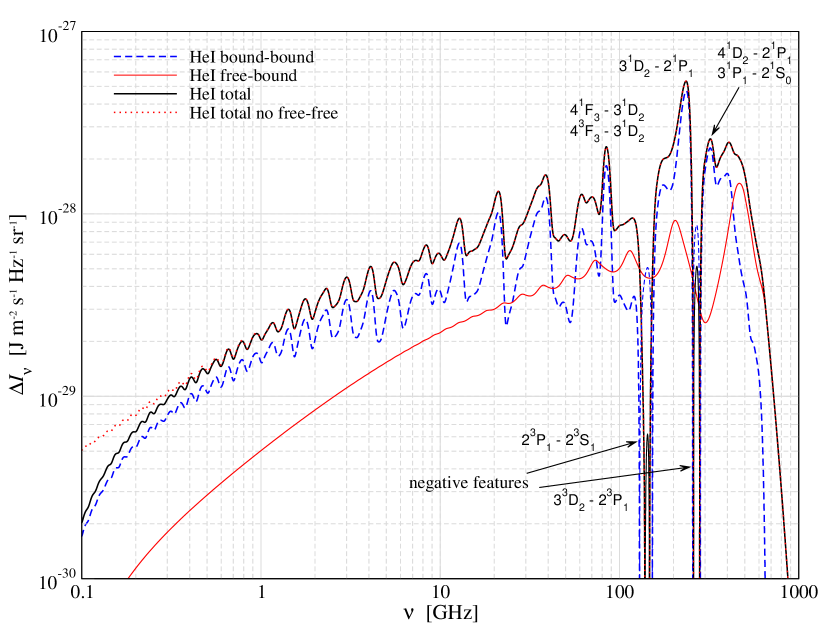
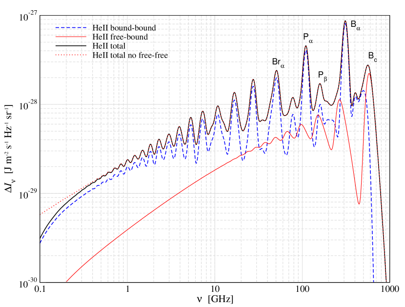
Figure 1: Cosmological recombination radiation from hydrogen and helium for 500 shells. He ii feedback and collisions were neglected and only the emission among levels with $n\geq 2$ is shown. For the total spectra we also illustrate the effect of free-free absorption.

4.2 Contributions from the three recombination eras

In Fig. 1, we illustrate the individual contributions from bound-bound and free-bound transitions of the three atomic species. We only show the emission among levels with $n\geq 2$, and do not display the high-frequency distortion from the Lyman lines and and 2s-1s continuum emission, though we compute them consistently as as part of the radiative transfer problem. The effect of collisions and He ii feedback were neglected to produce Fig. 1 and will be discussed below.

The hydrogen recombination radiation shows several feature (Balmer, Paschen and Brackett lines) related to the bound-bound $\alpha$ transitions ($\Delta n=1$), with the emission merging to a quasi-continuum at low frequencies. Free-free absorption is noticeable at $\nu\lesssim 0.3\,{\rm GHz}$. Although on average at a $\simeq 13$ times lower level, the distortions from the two helium eras also show significant structure. For the He ii spectrum, the effect of electron scattering is important, but nevertheless distinct features remain visible. The total He i spectrum, shows absorption features at $\nu\simeq 145\,{\rm GHz}$ and $\nu\simeq 270\,{\rm GHz}$. The first feature is related to the 10 830 $\AA$ line ($\leftrightarrow 2^{3}{\rm P}_{1}-2^{3}{\rm S}_{1}$) and the second to absorption in the 3D-2P triplet-triplet transitions (see Rubiño-Martín et al., 2008, for more details). For the helium contributions, free-free absorption becomes significant at $\nu\lesssim 0.5\,{\rm GHz}$, exponentially cutting off all recombination emission at $\nu\lesssim 50-100\,{\rm MHz}$.

In Figure 2, we show the total (bound-bound and free-bound) recombination radiation from hydrogen and helium for our detailed 500-shell calculations. We also included the high-frequency distortion, which for the helium spectra is strongly absorbed and reprocessed, reappearing as pre-recombination hydrogen Lyman-$\alpha$ emission (Rubiño-Martín et al., 2008; Chluba et al., 2012). Overall, the effect of helium is visible in several bands, introducing features, shifts in the line positions and enhanced emission. In particular, when adding all feedback corrections (see below for more discussion), the effect of helium becomes significant, in some parts well in excess of the expected average $\simeq 16\%$ contribution. This will help significantly when attempting to use the CRR to determine the pre-stellar (un-reprocessed) helium abundance.

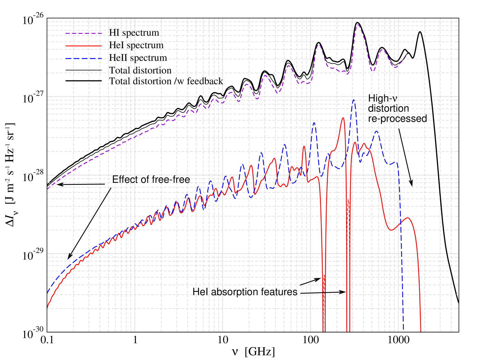
Figure 2: Cosmological recombination radiation from hydrogen and helium for 500-shell calculations. The different curves show individual contributions (without feedback) as well as the total distortion with and without feedback processes. At low frequencies, free-free absorption becomes noticeable. The effect is stronger for the contributions from helium due to the larger free-free optical depth before recombination ends at $z\simeq 10^{3}$. In total, some $6.1\,\gamma$ are emitted per hydrogen atom when all emission and feedback are included. Hydrogen alone contributes about $5.4\,\gamma/N_{\rm H}$ and helium $0.7\,\gamma/N_{\rm H}$ ($\simeq 8.9\,\gamma/N_{\rm He}$).

4.3 Effect of He ii feedback

As explained in Sect. 3.4, feedback caused by high-frequency photons emitted during the $\text{He\,{iii}}\rightarrow\text{He\,{ii}}$ recombination era changes the CRR of hydrogen and neutral helium by ionizing neutral atoms in their pre-recombination eras (Chluba & Sunyaev, 2010). In Fig. 3, we illustrate the effect on the hydrogen bound-bound spectrum. Since the number of helium atoms is lower than the number of hydrogen atoms, the effect is not as large, however, additional features appear in the recombination spectrum, e.g., around $\nu\simeq 200\,{\rm GHz}$ and $1\,{\rm THz}$. The dominant additional feedback is due to the reprocessing of the He ii Lyman-$\alpha$ line by He i continuum absorption. This causes pre-recombination emission of He i which then feeds back in the H i Lyman-continuum around $z\simeq 2500-3000$ (Chluba & Sunyaev, 2010). For comparison, we also show the case without any feedback at all (dashed/blue) and including primary He i photon feedback (dotted/violet). The latter case already goes beyond the calculations of (Rubiño-Martín et al., 2008), which neglected the feedback from the He i $2^{1}{\rm S}_{0}-1^{1}{\rm S}_{0}$ two-photon continuum.

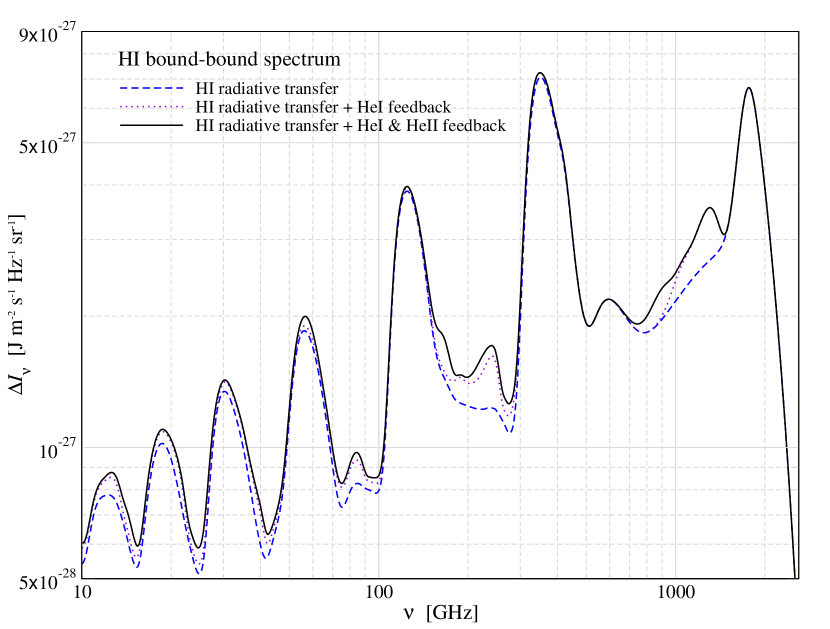
Figure 3: Helium feedback corrections to the H i bound-bound recombination radiation. The conductances were computed for $n_{\rm max}=500$. The main features due to helium feedback are in good agreement with the 20-shell calculations of Chluba & Sunyaev (2010).

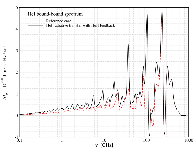
Figure 4: Helium feedback corrections to the He i bound-bound recombination radiation. The conductances were computed for $n_{\rm max}=500$. The main features due to He ii feedback are in good agreement with the 20-shell calculations of Chluba & Sunyaev (2010).

The effect on the He i recombination spectrum is much more dramatic (see Fig. 4). This is because in contrast to the feedback for hydrogen there is roughly one feedback photon per helium atom. The feedback occurs mainly around $z\simeq 4000-5000$ and is dominated by the He ii Lyman-$\alpha$ (Chluba & Sunyaev, 2010). Overall, He ii feedback enhances the total number of photons emitted by helium itself from $\simeq 6.7\,\gamma/N_{\rm He}$ to $\simeq 8.9\,\gamma/N_{\rm He}$. We included all free-bound and bound-bound emission of helium atoms in this estimate. Without He ii feedback, hydrogen emits roughly $5.3\,\gamma/N_{\rm H}$, which with feedback increases to $\simeq 5.4\,\gamma/N_{\rm H}$. In total, $\simeq 6.1\,\gamma/N_{\rm H}$ are emitted in the standard recombination process, with $\simeq 0.7\,\gamma/N_{\rm H}$ contributed by helium alone.

4.4 Derivatives with respect to $Y_{\rm p}$, $N_{\rm eff}$ and $\Omega_{\rm b}h^{2}$

As illustrated in Chluba & Sunyaev (2008b), the CRR directly depends on parameters like the CMB monopole temperature, $T_{0}$, the baryon density, $\Omega_{\rm b}h^{2}$, and the expansion rate today, $h$. Similarly, the helium mass fraction, $Y_{\rm p}$, and other parameters affecting the expansion rate, such as the cold dark matter density, $\Omega_{\rm c}$, and effective number of neutrino species, $N_{\rm eff}$, modify the CRR. Although detailed parameter forecasts and consideration of optimal experimental design will be left for future work, here we illustrate how the CRR depends on $\Omega_{\rm b}h^{2},Y_{\rm p}$ and $N_{\rm eff}$. Collisions are neglected in the calculation.

In Fig. 5 we show the logarithmic derivatives of the CRR with respect to $\Omega_{\rm b}h^{2}$ (keeping a flat Universe by varying $\Omega_{\Lambda}$), $Y_{\rm p}$ and $N_{\rm eff}$. For comparison, we also show the CRR itself. The logarithmic derivative with respect to $\Omega_{\rm b}h^{2}$ has a similar amplitude and shape as the CRR. This is expected since to leading order the total emission is simply proportional to the number of baryons in the Universe, i.e., $\Delta I_{\nu}^{\rm CRR}\propto\Omega_{\rm b}h^{2}$. The differences relative to the CRR are due to changes in the recombination dynamics and at low frequencies the efficiency of free-free absorption.

The logarithmic derivatives with respect to $Y_{\rm p}$ and $N_{\rm eff}$ show a much richer structure, with both positive and negative features. The CCR is much less sensitive to changes of $N_{\rm eff}$, since it only enters through the expansion rate. The helium abundance changes both the relative contribution of the two helium spectra to the hydrogen spectrum but also affects the recombination dynamics through feedback and modifications of the recombination rate. Naively, neglecting these dynamical aspects one would simply expect the total CRR to be the sum of the hydrogen and helium templates, which gives fewer features in the derivative (Fig. 6). Since the derivatives with respect to $Y_{\rm p}$, $N_{\rm eff}$ and $\Omega_{\rm b}h^{2}$ have very different shapes, it is clear that the CRR will help break degeneracies between these parameters. To what extent and with which strategy this may be possible will be studied in detail in a future paper.

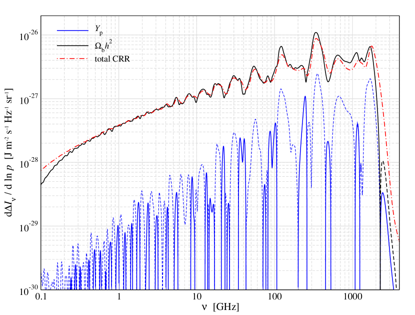
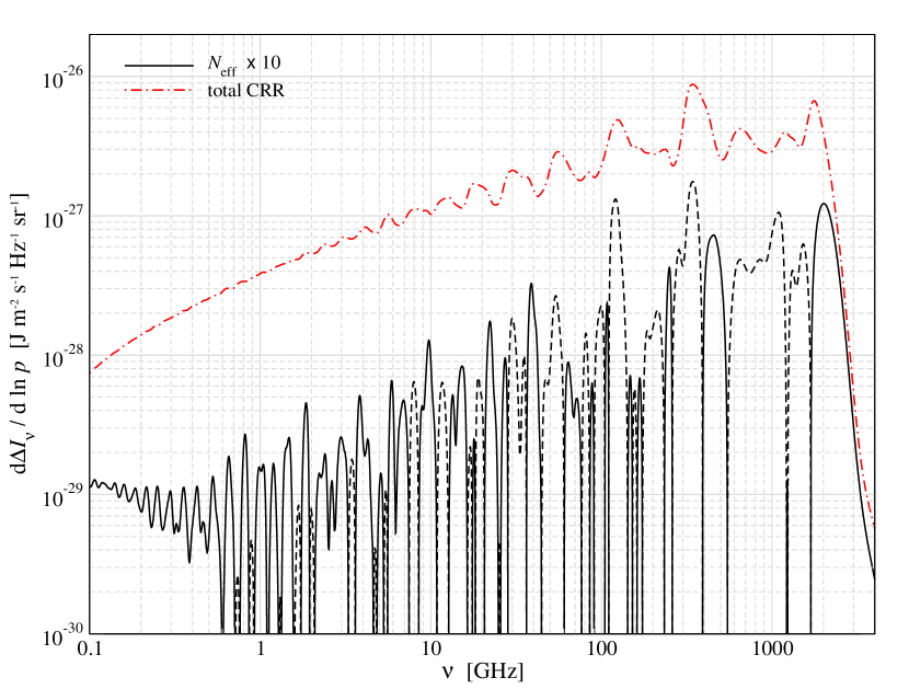
Figure 5: Logarithmic derivatives, ${\,\rm d}I_{\nu}/{\,\rm d}\ln p$, of the total recombination spectrum with respect to $Y_{\rm p}$, $\Omega_{\rm b}h^{2}$ and $N_{\rm eff}$. The derivatives with respect to $Y_{\rm p}$ and $N_{\rm eff}$ exhibit many features with both positive (solid line) and negative (dashed line) parts. We multiplied the derivative with respect to $N_{\rm eff}$ by a factor of 10 to make it visible on the same scale. For comparison we also show the total CRR itself.

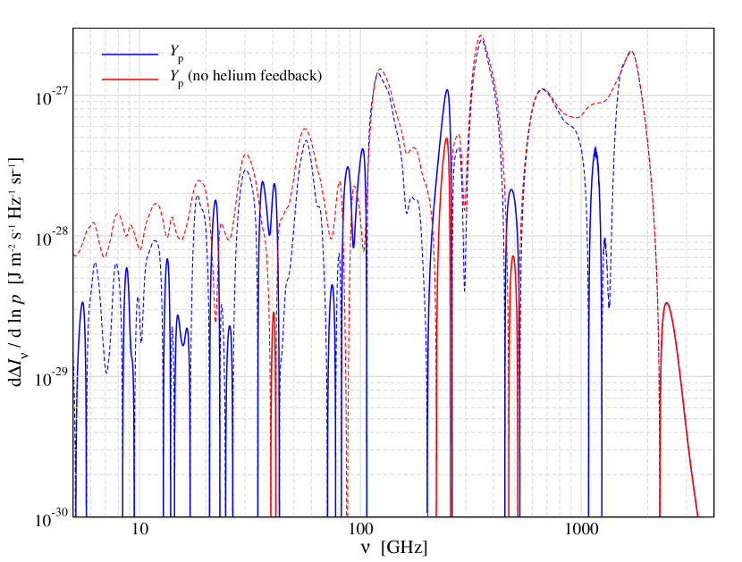
Figure 6: Logarithmic derivative, ${\,\rm d}I_{\nu}/{\,\rm d}\ln p$, of the total recombination spectrum with respect to $Y_{\rm p}$. We compare the case with and without helium feedback. Without helium feedback the derivative has less structure.

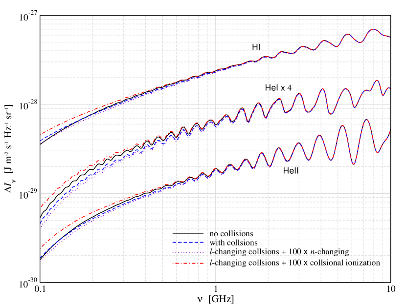
Figure 7: Effect of collisions on the recombination radiation for 100 atomic shells. Only $\ell$-changing collisions turn out to be important. Enhancing the rates of $n$-changing collision and collisional ionization rates by a factor of 100 makes their effect visible at low frequencies. We multiplied the He i spectrum by 4 to separate it from the He ii spectrum.

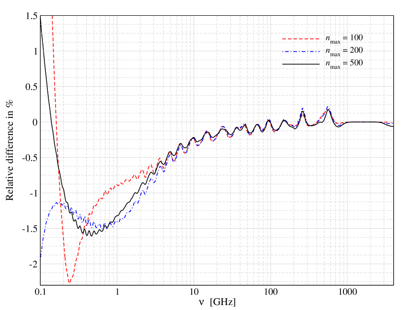
Figure 8: Relative change in the total recombination radiation caused by collisions for different number of shells. The spectrum without collisions is chosen as a reference.

4.5 Effect of collisions

The main effect of $\ell$-changing collisions is to push the angular-momentum substates within a given shell into statistical equilibrium. This enhances the very low-frequency emission ($\nu\lesssim 0.1\,{\rm GHz}$) while slightly lowering the emission at higher frequencies. This is because radiative recombinations are more efficient to the low-$\ell$ states ($\ell/n\simeq 0.1-0.2$), which in the absence of collisions are slightly overpopulated in comparison to the high-$\ell$ states. Low-$\ell$ states depopulate via large $\Delta n$ transitions, emitting at high frequencies, whereas transitions among high-$\ell$ states, due to dipole selection rules, are restricted to smaller $\Delta n$ jumps, emitting at lower frequencies. The $\ell$-changing collisions tend to level the low-$\ell$/high-$\ell$ population imbalance and hence enhance the low-frequency emission (see also, Chluba et al., 2007).

Collisional excitations and de-excitations push the relative populations of excited levels closer to Boltzmann equilibrium at the gas temperature, which is very close to the CMB temperature at the relevant redshifts. This therefore lowers the net radiative transition rate, which is proportional to the departure of the level populations from Boltzmann equilibrium with one another.

At low $n$, the populations are closer to Boltzmann equilibrium relative to the lowest ($n=2$) excited states, while at high $n$ they are closer to Saha equilibrium with the continuum. Collisional ionizations and three-body recombinations drive the highly-excited states even closer to Saha equilibrium with the continuum, steepening the level of departures from Saha equilibrium from low (largest departure) to high $n$ (smallest departure), leaving the low-$n$ states mostly unaffected. This has two effects. First, it reduces the net free-bound emission, which is proportional to the population departure from Saha equilibrium. Second, it enhances the bound-bound emission, which depends on the rate of change of population departures from equilibrium as a function of $n$.

All these effects are most significant at the low frequencies where the highly excited states radiate. They are also slightly more important for helium than for hydrogen, due to higher densities at the relevant times. In Fig. 7, we illustrate these effects using 100-shell calculations. We find $n$-changing collisions and collisional ionization to be subdominant, even for the He ii recombination radiation. Increasing these collision rates by two orders of magnitude makes their effect visible at low frequencies (see figure). The mixing of $\ell$ sub-levels produces a correction to the low-frequency recombination radiation, which for the He i spectrum becomes slightly more noticeable (in the total CRR of He i $\simeq 5\%$ as opposed to $\simeq 1.5\%$ for H i and He ii). However, in all cases the emission at $\nu\gtrsim 5-10\,{\rm GHz}$ remains practically unaffected.

In Fig. 8, we show the correction to the total CRR caused by collisions. We vary the number of shells in the calculation, to illustrate the changes at low and high frequencies. At low frequencies ($\nu\lesssim 1-2\,{\rm GHz}$), the effect reaches percent-level, while at higher frequencies it remains $\lesssim 0.5\%$, nearly independent of $n_{\rm max}$. This shows that collisional processes need to be taken into account for precise computations of the recombination radiation. For baseline calculations we neglect collisions, which implies an uncertainty at percent level for the total CRR.

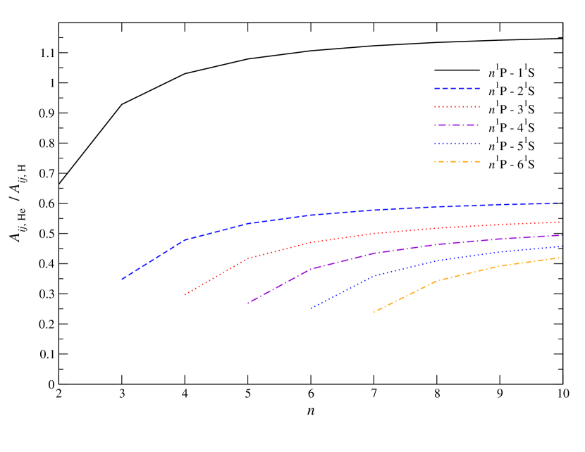
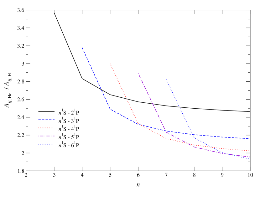
Figure 9: Comparison of the He i singlet transitions rates for the $n$P-$n^{\prime}$S and $n$S-$n^{\prime}$P series taken from the multiplet tables of Drake & Morton (2007) with the hydrogenic approximation.

4.6 Uncertainties due to the neutral helium model

As mentioned above, the atomic model for neutral helium is not as accurate as those of hydrogen and singly-ionized helium. This implies that the neutral helium contributions to the CRR is also uncertain. Here, we illustrate some of the crucial aspects and estimate the level of the uncertainty.

At this point, the level energies are probably the most certain. For $n\leq 10$, we compared the hydrogenic approximation and quantum defect energies with the data from Drake & Morton (2007). The biggest deviations are found for the $n$S and $n$P states, which at $n=10$ depart from the hydrogenic values by $\lesssim 6\%$. The energy values are matched very well by the quantum defect calculation, which is used to extrapolate to higher levels. For $\ell>1$, we find levels with $n\simeq 10$ to depart from the hydrogenic values by $\lesssim\rm few\times 10^{-4}$.

A larger uncertainty is found for the dipole transition rates among low-$\ell$ level involving $n$S, $n$P and $n$D states. In Fig. 9 we compare the transitions rates from Drake & Morton (2007) for the singlet $n$P-$n^{\prime}$S and $n$S-$n^{\prime}$P series with the hydrogenic approximation, $A^{\rm He}_{ij}\simeq(\nu^{\rm He}_{ij}/\nu_{\rm ij}^{\rm H})^{2}\,A^{\rm H}_{ij}$. This approximation works quite well for the $n$P-1S sequence, converging to the hydrogenic approximation at the $\simeq 10\%$ level for $n\simeq 10$. However, for the other cases, the hydrogenic approximation is significantly off, overestimating the transition rates for the $n$P-$n^{\prime}$S sequence roughly twice and underestimating the $n$S-$n^{\prime}$P sequence by a factor of $\simeq 2$ around $n\simeq 10$. For the triplet levels, we find a similar mismatch. For singlet transitions involving $n$D states, the hydrogenic approximation becomes accurate at the level of $\simeq 20\%-30\%$. Transition series involving only higher $\ell$ states approach hydrogenic values at the percent level. Overall, our analysis implies that low-$\ell$ transitions starting with $n>10$ and ending at $n^{\prime}\lesssim 10$ are not well approximated using hydrogenic values and an improved neutral helium model including many shells is ultimately needed.

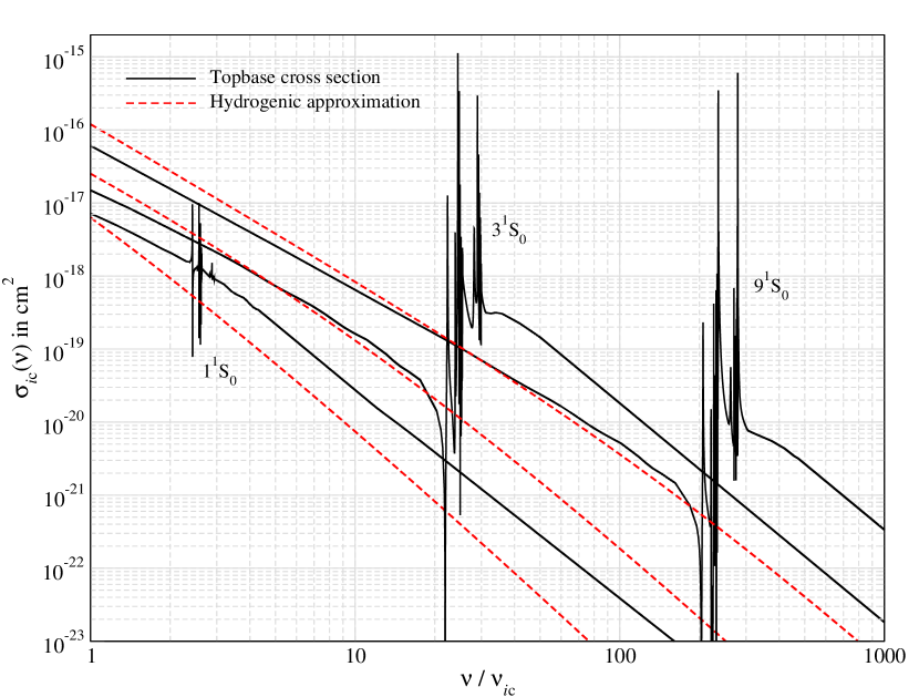
Figure 10: Comparison of photonionization cross sections from Topbase with simple rescaled hydrogenic approximations. Agreement with the hydrogenic approximation close to the ionization threshold could be achieved by matching the cross section, but even the slopes do not match well.

As mentioned above, the photonionization cross sections are probably the largest source of uncertainty in the neutral helium model. This is because the hydrogenic approximation neglects corrections to the shape of the cross section from the non-hydrogenic character of the wave-functions and due to auto-ionization resonances, which are important for the low-$\ell$ states ($n$S, $n$P and $n$D). This is illustrated in Fig. 10, where we compare the TopBase cross section with the hydrogenic approximation for some examples. We find that even for $n\simeq 10$, the cross sections for the $n$S and $n$P states show clear non-hydrogenic character already close to the threshold frequency. Although we do not expect auto-ionization resonances to significantly contribute to the total photoionization and recombination rates (which could have an effect on the recombination dynamics) they affect the precise shape of the He i free-bound continuum. Similarly, for the $n$S and $n$P states we find the slopes of the cross section to be more shallow than the hydrogenic approximation. For the $n$D states, the match is found to be much better already, but auto-ionization resonances are still present even there. For the triplet $n$P states, TopBase cross sections only exist for $n=2$ and $n=3$. Thus, the shape of the free-bound continuum for $n>3$ is likely affected at a significant level. For $n>9$, we also expect the free-bound continuua to show dependence on the shortcomings of the hydrogenic approximation. A improved quantum mechanical model of neutral helium will therefore eventually be needed for highly accurate predictions of the CRR.

5 Conclusions and future work

We carried out the first comprehensive computation of the CRR from hydrogen and helium including all relevant processes for 500-shell atoms. Our computations improve over previous calculations in terms of the total number of included shells and the modeling of feedback processes. For the first time, we include the free-bound emission from helium and model the effect of collisional processes at high redshift. We furthermore overcome the performance-bottleneck of previous treatments using effective multilevel atom and conductance methods. With CosmoSpec one calculation of the CRR now only takes $\simeq 15$ seconds on a standard laptop. This opens a way to more detailed forecasts and parameter explorations with the CRR, applications that we will address in a future paper.

The precision of our calculations is currently limited by the atomic model for neutral helium (see Sect. 4.6 for more detailed discussion) and uncertainties due to collisions. For neutral helium, uncertainties related to the photoionization cross section in particular are expected to exceed the level of 10%-30% for the He i free-bound continuum. This should enter the total CRR at the level of a few percent. Similarly, transition rates, multiplet ratios and radiative/collisional singlet-triplet transitions among excited levels should be considered in more detail. For the total CRR, this implies an uncertainty at the level of a few percent. We also show that collisional mixing of $\ell$-substates is noticeable at low frequencies ($\nu\lesssim 2\,{\rm GHz}$). At higher frequencies, corrections due to collisions remain at the sub-percent level (Fig. 8).

Our calculations clearly highlight the importance of helium feedback for the detailed shape of the CRR (Fig. 3 and 4), which introduces additional features into the derivative of the CRR with respect to the helium abundance (Fig. 6). This process is thus required for a detailed modeling of the dependence of the CRR on the helium abundance, which may be used to extract this parameter from future spectral distortion measurements. The CRR may also help break degeneracies between $N_{\rm eff}$, $Y_{\rm p}$ and $\Omega_{\rm b}$ due to the differing sensitivity of the signal on these parameters. In combination with future CMB anisotropy and large-scale structure measurements (Abazajian et al., 2015), this could deliver additional constraints on neutrino physics.

Our calculations still use a few approximations that could affect the results at the level of $\simeq 1\%$. At this point, we did not separately include the effect of He ii Lyman-$\beta$. This will change the dynamics of He ii recombination by Lyman-$n$ feedback (Chluba & Sunyaev, 2007; Switzer & Hirata, 2008a; Ali-Haïmoud et al., 2010) and also modify the interspecies feedback slightly. Similarly, for the He ii recombination history we neglected detailed radiative transfer effects, stimulated He ii 2s-1s two-photon emission and Raman processes, all effects that were studied in detail for the hydrogen recombination history (Chluba & Sunyaev, 2006b; Kholupenko & Ivanchik, 2006; Hirata & Switzer, 2008; Chluba & Sunyaev, 2008c; Hirata, 2008). Corrections due to charge transfer between He ii and He i are expected to be small, however, in more detailed computations this processes should be considered. Also, one should treat the direct ionizations from the ground state and continuum escape more carefully.

The CRR probes the Universe at earlier stages than the CMB anisotropies, providing a new window for complementary constraints on non-standard physics. For instance, variations of fundamental constants, such as the fine-structure constant or electron-to-proton mass ratio, would shift the position and relative amplitudes of the recombination lines. We highlight that the effect of variations of $\alpha$ and $m_{\rm e}$ can be treated self-consistently using the effective rate and conductance method (see Appendix B). We find the effective recombination and photoionization rates to scale as $\alpha_{{\rm c}i}\propto\alpha^{2}m_{\rm e}^{-2}$ and $\beta_{i\rm c}\propto\alpha^{5}m_{\rm e}$, respectively. These effects have been incorporated by HyRec for a while, but they differ from previously adopted scalings (e.g., Kaplinghat et al., 1999; Scóccola et al., 2009). The differences may change the constraints derived from Planck data (Planck Collaboration et al., 2015b).

Another interesting effect is the extra ionization and excitation from annihilating or decaying dark matter particles, which could significantly enhance the CRR. It may therefore be possible to derive interesting upper limits on dark matter properties with future spectral distortion measurements, even in the absence of a detection. Tests of spatial variations in the composition of the Universe, for example, due to non-standard BBN models or cosmic bubble collisions (Dai et al., 2013; Silk & Chluba, 2014; Chary, 2015) may be another line of research. We look forward to exploring these directions in the future.

Appendix A Improved $J$-resolved transitions rates from hydrogenic values

In the helium model of Rubiño-Martín et al. (2008), transitions among triplet states with $n\leq 10$ which are not contained in the multiplet tables of Drake & Morton (2007) are filled with hydrogenic values using the approximation

$$A^{\rm He}_{nLJ\rightarrow n^{\prime}L^{\prime}J^{\prime}} \approx\frac{(2J^{\prime}+1)}{(2L^{\prime}+1)(2S^{\prime}+1)}\,A^{\rm H}_{nL\rightarrow n^{\prime}L^{\prime}}.$$ (9)

This approximation assumes that the partial rates for individual sub-levels within a multiplet are the same and that the total transition rate averaged over all $J$ and $J^{\prime}$ is given by the hydrogenic (non-$J$-resolved) values. This can be readily confirmed by computing the $J$-averaged transition rate

$$A^{\rm He}_{nL\rightarrow n^{\prime}L^{\prime}} =\sum_{JJ^{\prime}}\frac{(2J+1)}{(2L+1)(2S+1)}\,A^{\rm He}_{nLJ\rightarrow n^{\prime}L^{\prime}J^{\prime}}\approx A^{\rm H}_{nL\rightarrow n^{\prime}L^{\prime}}$$ (10)

after inserting Eq. (9). From the atomic physics point of view, this approximation is incorrect. It is well-known (e.g., Goldberg, 1935; Condon & Shortley, 1963) that the transitions within a given multiplet differ in strength and that their relative ratio deviates by much more than expressed with Eq. (9). Using the relation $\mathcal{S}_{ij}\propto\lambda^{3}g_{i}\,A_{ij}$, between the line strength $\mathcal{S}_{ij}$ and transition rate $A_{ij}$ together with the sum rule (e.g., see Edmonds, 1960)

$$\mathcal{S}_{nLJ\rightarrow n^{\prime}L^{\prime}J^{\prime}}=(2J+1)(2J^{\prime}+1)\left|{\left\{\begin{array}[]{ccc}L&J&S\\ J^{\prime}&L^{\prime}&1\end{array}\right\}}\right|^{2}\mathcal{S}_{nL\rightarrow n^{\prime}L^{\prime}},$$ (13)

where ${\left\{\begin{array}[]{ccc}a&b&c\\ d&e&f\end{array}\right\}}$ denotes the Wigner-6$J$-symbol, one can show that the transition rates within a multiplet should scale like

$$A^{\rm He}_{nLJ\rightarrow n^{\prime}L^{\prime}J^{\prime}}\approx(2L+1)(2J^{\prime}+1)\left|{\left\{\begin{array}[]{ccc}L&J&S\\ J^{\prime}&L^{\prime}&1\end{array}\right\}}\right|^{2}A^{\rm H}_{nL\rightarrow n^{\prime}L^{\prime}}.$$ (16)

For $\Delta L=-1$, we therefore have the three cases

$$r_{J-1} =\frac{(L+J+2)(L+J+1)(L+J-1)(L+J-2)}{4J(2J+1)\,L\,(2L-1)}$$ (17a)

$$r_{J} =\frac{(2J+1)(J-L-1)(L-J-2)}{(J+1)(L+J+1)(L+J-2)}\,r_{J-1}$$ (17b)

$$r_{J+1} =\frac{J(J-L)(L-J-3)}{(2J+1)(L+J-1)(L+J+2)}\,r_{J}$$ (17c)

for the line ratios $r_{k}=A^{\rm He}_{nLJ\rightarrow n^{\prime}L-1k}/A^{\rm H}_{nL\rightarrow n^{\prime}L-1}$. Within these multiplets, the strongest line is the one for $\Delta J=-1$, which for $L\gg 1$ roughly equals the hydrogenic value, $r_{J-1}\approx 1$. For large $L$, the intensity of the second line ($\Delta J=0$) drops like $r_{J}\approx L^{-2}$, while for the third line we have $r_{J+1}\approx 4L^{-4}$. Clearly, this is a very different behavior than obtained with Eq. (9). For $\Delta L=+1$, we similarly find the line ratios

$$r_{J-1} =\frac{(J+1)(J-L-3)(L-J)}{(2J+1)(L+J)(L+J+3)}\,r_{J}$$ (18a)

$$r_{J} =\frac{(2J+1)(L-J-1)(J-L-2)}{J(L+J+1)(L+J+4)}\,r_{J+1}$$ (18b)

$$r_{J+1} =\frac{(L+J+4)(L+J+3)(L+J+1)(L+J)}{4(2L+3)(L+1)(2J+1)(J+1)},$$ (18c)

where now the strongest line in the multiplet is the one for $\Delta J=+1$.

When considering transitions from levels with $n>10$ (non-$J$-resolved) to levels with $n^{\prime}\leq 10$ ($J$-resolved), we average Eq. (16) over the initial level $J$, giving us the approximation

$$A^{\rm He}_{nL\rightarrow n^{\prime}L^{\prime}J^{\prime}}\approx\frac{(2J^{\prime}+1)}{(2L^{\prime}+1)(2S^{\prime}+1)}\,A^{\rm H}_{nL\rightarrow n^{\prime}L^{\prime}},$$ (19)

which also follows from Eq. (9). Notice that to obtain the hydrogenic approximation we also scale by the average transition frequency ratio to the third power. This usually is a small correction.

We find that the changes to the recombination history and spectrum caused by the above improvements are small ($\lesssim 0.1\%$). The main reason is that only a few transitions among the high-$L$ states at $n\leq 10$ are missing from the multiplet tables of Drake & Morton (2007). In addition, for transitions between levels with $n>10$ (non-$J$-resolved) to levels with $n^{\prime}\leq 10$ ($J$-resolved) the approximation of Rubiño-Martín et al. (2008) already represented the correct value, as shown in Eq. (19). This explains why the overall correction remains small.

A.1 $J$-resolved photoionization cross sections

The total photoionization cross section from level $nLJ$ is the sum of the photoionization cross sections to continuum states (label “c”, with an implicit integration over final electron momentum) with angular momentum quantum numbers $L^{\prime}J^{\prime}$:

$$\sigma_{nLJ}=\sum_{L^{\prime}J^{\prime}}\sigma_{nLJ\rightarrow\textrm{c}L^{\prime}J^{\prime}},$$ (20)

where the spin quantum number $S$ is implicit and held fixed throughout. Each angular-momentum-resolved transition is proportional to the line strength $\mathcal{S}_{nLJ,\textrm{c}L^{\prime}J^{\prime}}$ (Condon & Shortley, 1963):

$$\sigma_{nLJ\rightarrow\textrm{c}L^{\prime}J^{\prime}}\propto\frac{\mathcal{S}_{nLJ,\textrm{c}L^{\prime}J^{\prime}}}{2J+1}.$$ (21)

Summing over final states, and using the sum rule (Edmonds, 1960)

$$\sum_{J^{\prime}}\mathcal{S}_{nLJ,\textrm{c}L^{\prime}J^{\prime}}=\frac{2J+1}{2L+1}\mathcal{S}_{nL,\textrm{c}L^{\prime}},$$ (22)

we arrive at

$$\sigma_{nLJ}\propto\frac{1}{2L+1}\sum_{L^{\prime}}\mathcal{S}_{nL,\textrm{c}L^{\prime}},$$ (23)

which is independent of $J$.

Appendix B Rescaling of the effective rates for hydrogenic ions

Noting that the dipole transition rates, $A_{i\rightarrow j}$ (between levels $i$ and $j$, where $i$ is the upper level) and photoionization cross sections, $\sigma_{i\rightarrow\rm c}$, scale as

$$A_{i\rightarrow j} \propto\sigma_{i\rightarrow\rm c}\nu^{2}{\,\rm d}\nu\propto\alpha\,\nu_{i\rightarrow j/{\rm c}}^{3}\,a_{0}^{2}\,Z^{-2}=\alpha^{5}\,m_{\rm e}\,Z^{4},$$ (25)

we find that the radiative rate coefficients scale as (compare, Ali-Haïmoud & Hirata, 2011)

$$R_{i\rightarrow j} =A_{i\rightarrow j}[1+n_{\nu_{ij}}(T_{\gamma})]=\alpha^{5}\,m_{\rm e}\,Z^{4}F\left(\frac{kT_{\gamma}}{h\nu_{ij}}\right)$$ (26a)

$$\beta_{i\rightarrow{\rm c}} =\frac{8\pi}{c^{2}}\int_{\nu_{i\rm c}}^{\infty}\nu^{2}\,\sigma_{i\rightarrow\rm c}(\nu)\,n_{\nu}(T_{\gamma}){\,\rm d}\nu=\alpha^{5}\,m_{\rm e}\,Z^{4}B\left(\frac{kT_{\gamma}}{h\nu_{i\rm c}}\right)$$ (26b)

$$\alpha_{{\rm c}\rightarrow i} =\frac{8\pi}{c^{2}}\,f_{i}^{\rm eq}(T_{\rm e})\int_{\nu_{i\rm c}}^{\infty}\nu^{2}\,\sigma_{i\rightarrow\rm c}(\nu)\,[1+n_{\nu}(T_{\gamma})]\,{{\rm e}^{-h\nu/kT_{\rm e}}}{\,\rm d}\nu$$

$$=\frac{\alpha^{2}\,Z}{m_{\rm e}^{2}}A\left(\frac{kT_{\gamma}}{h\nu_{i\rm c}},\frac{kT_{\rm e}}{h\nu_{i\rm c}}\right)$$ (26c)

$$f_{i}^{\rm eq}(T_{\rm e}) =\frac{g_{i}}{2g_{\rm c}}\frac{h^{3}\,{{\rm e}^{h\nu_{i\rm c}/kT_{\rm e}}}}{(2\pi m_{\rm e}kT_{\rm e})^{3/2}}.$$ (26d)

Here, $\alpha$ is the fine structure constant; $Z$ the charge of the hydrogenic ion; $m_{\rm e}$ its reduced mass; $a_{0}\simeq\alpha^{-1}m_{\rm e}^{-1}$ the Bohr radius; $\nu_{ij}\simeq\nu_{i\rm c}\simeq\alpha^{2}m_{\rm e}\,Z^{2}$ the bound-bound / bound-free transition frequency, respectively; $n_{\nu}(T_{\gamma})=1/({{\rm e}^{h\nu/kT_{\gamma}}}-1)$ the blackbody photon occupation number; $g_{i}$ and $g_{\rm c}$ the statistical weights of the level $i$ and the continuum particle.

The inverse dipole transitions rate, $R_{j\rightarrow i}$, is simply given by $R_{j\rightarrow i}=\frac{g_{i}}{g_{j}}R_{i\rightarrow j}\,{{\rm e}^{-h\nu_{ij}/kT_{\gamma}}}$. Because the probabilities of an electron reaching a specific level $i$ from another level $j$ within the excited levels just depends on ratios and sums of $R_{i\rightarrow j}$ and $\beta_{i\rightarrow{\rm c}}$, the effective rate coefficients $\mathcal{A}_{i}(T_{\gamma},T_{\rm e})$, $\mathcal{B}_{i}(T_{\gamma})$ and $\mathcal{R}_{i\rightarrow j}(T_{\gamma})$ (Eq. 17, 18 and 19 of Ali-Haïmoud & Hirata, 2011) for any hydrogenic ion can be obtained from those of hydrogen. Defining the factors $f_{\mathcal{A}}=\alpha^{2}\,Z\,\mu^{2}_{\rm H}/[\alpha^{2}_{\rm ref}\,\mu^{2}_{Z}]$, $f_{\mathcal{B}}=\alpha^{5}\,Z^{4}\,\mu_{Z}/[\alpha^{5}_{\rm ref}\,\mu_{\rm H}]$ and $f_{T}=\alpha^{2}_{\rm ref}\,\mu_{\rm H}/[\alpha^{2}Z^{2}\,\mu_{Z}]$, we find

$$\mathcal{A}_{i}(T_{\gamma},T_{\rm e}) =f_{\mathcal{A}}\,\mathcal{A}^{\rm H}_{i}\left(f_{T}T_{\gamma},f_{T}T_{\rm e}\right)$$ (27a)

$$\mathcal{B}_{i}(T_{\gamma}) =f_{\mathcal{B}}\,\mathcal{B}^{\rm H}_{i}\left(f_{T}T_{\gamma}\right)$$ (27b)

$$\mathcal{R}_{i\rightarrow j}(T_{\gamma}) =f_{\mathcal{B}}\,\mathcal{R}^{\rm H}_{i\rightarrow j}\left(f_{T}T_{\gamma}\right),$$ (27c)

where $\mu_{\rm H}$ and $\mu_{Z}$ are the reduced masses of hydrogen and the hydrogenic ion with charge $Z$ in units of the electron rest mass. We also included the explicit dependence on $\alpha$, where $\alpha_{\rm ref}\approx 1/137$ is the valued used for the effective rate computation.

The effective conductances of hydrogenic helium can be similarly obtained with

$$\mathcal{G}^{\rm e}_{n^{\prime}n}(T_{\gamma}) =f_{\mathcal{B}}\,\mathcal{G}^{\rm e,H}_{n^{\prime}n}\left(f_{T}T_{\gamma}\right)$$ (28a)

$$\mathcal{G}^{i}_{n^{\prime}n}(T_{\gamma}) =f_{\mathcal{B}}\,\mathcal{G}^{i,\rm H}_{n^{\prime}n}\left(f_{T}T_{\gamma}\right)$$ (28b)

$$\frac{{\,\rm d}\mathcal{G}^{i}_{\rm fb}(T_{\gamma})}{{\,\rm d}\nu} =f_{\mathcal{B}}\,\frac{{\,\rm d}\mathcal{G}^{i,\rm H}_{\rm fb}}{{\,\rm d}\nu}\left(f_{T}T_{\gamma}\right)$$ (28c)

using those of hydrogen (superscript ’H’) with the notation of Ali-Haïmoud (2013) for the conductances. In addition, we need to shift the energies of each frequency bin in the conductance table. These simple scalings are no longer exactly valid when collisions are included (Sect. 3.5). They also neglect smaller corrections due to the Lamb-shift, which depend on $\alpha$ as well.

Appendix C Classical derivation of $\ell$-changing collisional transition rates

In this Appendix, we give a simple derivation of the classical result of Vrinceanu et al. (2012) in the Born approximation. We recover the leading term of their classical result up to corrections of order $1/n\ll 1$.

Let us consider an electron moving in a Keplerian orbit around a nucleus with charge $Z_{\rm nuc}$, and subject to a perturbing force per unit mass $\boldsymbol{f}(\boldsymbol{r},t)$ acting on the electron. We have $Z_{\rm nuc}=2$ for singly-ionized helium and 1 for hydrogen and neutral helium, for which we approximate the helium nucleus and inner electron as a point charge, and the orbiting electron is the outermost, excited one.

The Gaussian perturbation equation (see e.g. Roy, 1982) for the osculating orbital elements $c_{i}$ are

$$\frac{{\,\rm d}c_{i}}{{\,\rm d}t}=\frac{\partial c_{i}}{\partial\boldsymbol{\varv}}\cdot\boldsymbol{f}.$$ (29)

We emphasize that these equations are exact. We define $\kappa\equiv Z_{\rm nuc}q_{\rm e}^{2}/m_{\rm e}$, where $q_{\rm e}$ is the elementary charge and $m_{\rm e}$ is the reduced mass of the electron-nucleus system. The energy per unit mass is $\epsilon=\frac{1}{2}\varv^{2}-\kappa/r$, and evolves under the influence of the perturbing force according to

$$\frac{{\,\rm d}\epsilon}{{\,\rm d}t}=\boldsymbol{\varv\cdot f},$$ (30)

and the angular momentum per unit mass $\boldsymbol{L}\equiv\boldsymbol{r}\times\boldsymbol{\varv}$ evolves according to

$$\frac{{\,\rm d}\boldsymbol{L}}{{\,\rm d}t}=\boldsymbol{r}\times\boldsymbol{f}.$$ (31)

We now make two assumptions:
$(i)$ We assume that the perturbing force is nearly constant accross the orbit of the electron. For the problem of interest ($\boldsymbol{f}$ generated by a passing ion), this is equivalent to the electric dipole approximation, where we assume that the dimensions of the orbit are much smaller than the impact parameter, $b$.
$(ii)$ We assume that the force varies on a timescale long compared to the orbital period. This is the orbital adiabatic approximation, and it requires that $\varv/b\ll\nu_{n,n\pm 1}$, where $\nu_{n,n\pm 1}$ is the transition frequency from $n$ to the neighboring energy states.

With these assumptions, one can average the rate of change of orbital elements over one orbit, and obtain, first, that the energy $\epsilon$ is conserved, and second, that the secular rate of change of angular momentum is

$$\Bigg{\langle}\frac{{\,\rm d}\boldsymbol{L}}{{\,\rm d}t}\Bigg{\rangle}=\langle\boldsymbol{r}\rangle\times\boldsymbol{f},$$ (32)

where $\langle\boldsymbol{r}\rangle$ is the time-average of the position vector over one orbit. Note that this reduces to the standard formula for a torque on an electric dipole moment when $m_{\rm e}\boldsymbol{f}=q_{\rm e}\boldsymbol{E}$.

The time-averaged position vector for a Keplerian orbit can be shown to be $\langle\boldsymbol{r}\rangle=-(3/2)a\boldsymbol{e}$, where $a$ is the semi-major axis and $\boldsymbol{e}$ is the eccentricity vector, pointing from the orbital focus to percienter, and having magnitude $e<1$, the orbital eccentricity. The secular rate of change of angular momentum is therefore

$$\Bigg{\langle}\frac{{\,\rm d}\boldsymbol{L}}{{\,\rm d}t}\Bigg{\rangle}=\frac{3}{2}a\boldsymbol{f}\times\boldsymbol{e}.$$ (33)

One can derive a similar expression for the rate of change of the eccentricity vector itself,

$$\Bigg{\langle}\frac{{\,\rm d}\boldsymbol{e}}{{\,\rm d}t}\Bigg{\rangle}=\frac{3}{2\kappa}\boldsymbol{f}\times\boldsymbol{L},$$ (34)

though we will not need it in the Born approximation.

We now specify to the perturbing force created by a passing ion of charge $Z_{\rm ion}q_{\rm e}>0$, moving on a trajectory $\boldsymbol{R}(t)$:

$$\boldsymbol{f}=\frac{Z_{\rm ion}q_{\rm e}^{2}}{m_{\rm e}}\frac{\hat{R}}{R^{2}}.$$ (35)

The specific angular momentum $L_{\rm ion}$ of the ion-nucleus system is conserved in the collision (up to corrections of order $\hbar$). Defining $\Phi$ as the polar angle of the passing ion, which starts at $\Phi=0$, we have $L_{\rm ion}=R^{2}\dot{\Phi}=b\varv$, where $b$ is the impact parameter and $\varv$ the velocity of the ion at infinity. We may therefore rewrite the perturbing force as

$$\boldsymbol{f}=\frac{Z_{\rm ion}q_{\rm e}^{2}}{m_{\rm e}b\varv}\dot{\Phi}\left[\cos\Phi~{}\hat{x}+\sin\Phi~{}\hat{y}\right],$$ (36)

where $\hat{x},\hat{y}$ form a fixed orthonormal basis in the plane of the ion’s orbit, with $\hat{x}$ pointing in the incoming direction of the ion.

We now define the dimensionless angular momentum

$$\boldsymbol{l}\equiv\frac{\boldsymbol{L}}{\sqrt{\kappa a}},$$ (37)

whose magnitude is $l=\sqrt{1-e^{2}}$. In terms of quantum numbers for a hydrogenic atom, $l=\ell/n$. The secular equation can be rewritten as

$$\frac{{\,\rm d}\boldsymbol{l}}{{\,\rm d}\Phi}=\alpha\left[\cos\Phi~{}\hat{x}+\sin\Phi~{}\hat{y}\right]\times\boldsymbol{e},$$ (38)

where

$$\alpha\equiv\frac{3}{2}\sqrt{\frac{a}{\kappa}}\frac{Z_{\rm ion}q_{\rm e}^{2}}{m_{\rm e}b\varv}.$$ (39)

So far we have not made any approximation besides the orbital adiabatic and electric dipole approximations. We now make the Born approximation, i.e. we assume that the perturbation is small enough that $\boldsymbol{e}$ can be approximated as constant in the above equation. This is equivalent to a first-order expansion in the small parameter $\alpha\ll 1$. We also assume that the ion’s trajectory can be approximated as a straight line, with final polar angle $\Phi_{f}=\pi$. This is accurate for neutral hydrogen and helium (up to small deflections due to the induced polarization of the atom by the passing ion). It is not necessarily so for singly-ionized helium, in which case the ion’s orbit is a hyperbola. We shall argue later on that for the conditions relevant to this problem the deflection angle is very small and the straight line approximation should be very accurate, even for singly-ionized helium.

Integrating Eq. (38) from $\Phi=0$ to $\pi$, we get

$$\Delta\boldsymbol{l}=2\alpha e~{}\hat{y}.$$ (40)

The change of the magnitude of $\boldsymbol{l}$ is therefore to first order in $\alpha$,

$$\Delta l=2\alpha e~{}\hat{y}\cdot\hat{l}.$$ (41)

When considering all orientations of the system, the scalar product $\hat{y}\cdot\hat{l}$ is uniformly distributed between -1 and 1. Therefore, at fixed $b$ and $\varv$, the differential probability to change the angular momentum by $\Delta l$ is

$$\frac{{\,\rm d}P}{{\,\rm d}\Delta l}=\begin{cases}\frac{1}{4\alpha e}&\ \text{if}\ |\Delta l|\leq 2\alpha e,\\ 0&\text{otherwise}.\end{cases}$$ (42)

The differential collision rate is then obtained from integrating over impact parameters and velocities:

$$\frac{{\,\rm d}C}{{\,\rm d}\Delta l}=N_{\rm ion}\int{\,\rm d}^{3}\varv~{}\varv f_{\rm ion}(\varv)\int 2\pi b{\,\rm d}b\frac{{\,\rm d}P}{{\,\rm d}\Delta l},$$ (43)

where $f_{\rm ion}(\varv)$ is the Maxwell-Boltzmann probability distribution for the velocity $\varv$ of the ion relative to the target,

$$f_{\rm ion}(\varv)\equiv\left(\frac{M}{2\pi kT}\right)^{3/2}\exp\left[-\frac{M\varv^{2}}{2kT}\right],$$ (44)

where $M$ is the reduced mass of the ion-target system. Changing integration variables from $b$ to $\alpha$, we arrive at

$$\frac{{\,\rm d}C}{{\,\rm d}\Delta l}=N_{\rm ion}2\pi\left(\frac{3}{2}\sqrt{\frac{a}{\kappa}}\frac{Z_{\rm ion}q_{\rm e}^{2}}{m_{\rm e}}\right)^{2}\int\frac{{\,\rm d}^{3}\varv}{\varv}f_{\rm ion}(\varv)\int\frac{{\,\rm d}P}{{\,\rm d}\Delta l}\frac{{\,\rm d}\alpha}{\alpha^{3}}.$$ (45)

For any given $\Delta l$, the classical transition probability is non-vanishing only for $\alpha\geq|\Delta l|/(2e)$, and we therefore obtain

$$\int\frac{{\,\rm d}P}{{\,\rm d}\Delta l}\frac{{\,\rm d}\alpha}{\alpha^{3}}=\frac{1}{4e}\int_{|\Delta l|/(2e)}\frac{{\,\rm d}\alpha}{\alpha^{4}}=\frac{2}{3}\frac{1-l^{2}}{|\Delta l|^{3}},$$ (46)

where we used $l^{2}+e^{2}=1$. This is the first term in the semi-classical expansion of Vrinceanu et al. (2012) [their Eq. (7)], the next terms being suppressed by higher orders in $|\Delta l|\ll 1$. Integrating over velocities and inserting the value of $\kappa$, we obtain

$$\frac{{\,\rm d}C}{{\,\rm d}\Delta l}=N_{\rm ion}\frac{3a}{Z_{\rm nuc}}\frac{(Z_{\rm ion}q_{\rm e})^{2}}{m_{\rm e}}\sqrt{\frac{2\pi M}{kT}}\frac{1-l^{2}}{|\Delta l|^{3}}.$$ (47)

Finally, substituting $a=n^{2}a_{0}/Z_{\rm nuc}$, where the Bohr radius is

$$a_{0}=\frac{\hbar^{2}}{m_{\rm e}q_{\rm e}^{2}},$$ (48)

and replacing $l=\ell/n$, we get our final expression,

$$\frac{{\,\rm d}C}{{\,\rm d}\Delta\ell}=N_{\rm ion}\frac{Z_{\rm ion}^{2}}{Z_{\rm nuc}^{2}}\,3n^{4}\frac{\hbar^{2}}{m_{\rm e}^{2}}\sqrt{\frac{2\pi M}{kT}}\frac{1-(\ell/n)^{2}}{|\Delta\ell|^{3}}.$$ (49)

We emphasize that this is a differential transition rate, since classically $\ell$ is a continuous number.

To get the expression of Vrinceanu et al. (2012), we approximate

$$C_{n\ell\rightarrow n\ell^{\prime}}\approx\frac{{\,\rm d}C}{{\,\rm d}\Delta\ell}(\Delta\ell=\ell^{\prime}-\ell).$$ (50)

This expression is of course expected to be only accurate within order unity factors. As shown by Vrinceanu et al. (2012), their expression reproduces the full quantum calculations for $\Delta\ell>1$ extremely well.

C.1 A note on hyperbolic trajectories

We have assumed that the trajectory of the colliding ion relative to the target nucleus is a straight line. In the case of singly-ionized helium, the target is charged and the orbit is in fact a hyperbola. One can show in this case that the final polar angle $\Phi_{f}$ is such that

$$\tan(\Phi_{f}/2)=\frac{Mb\varv^{2}}{Z_{\rm ion}q_{\rm e}^{2}}=\frac{3}{2\alpha}\frac{M}{m_{\rm e}}\frac{\varv}{\sqrt{2|\epsilon|}}.$$ (51)

Now taking $\varv\sim\sqrt{kT/M}$ and $|\epsilon|=E_{\rm I}/(n^{2}m_{\rm e})$, where $E_{\rm I}$ is the ionization energy, we obtain

$$\tan(\Phi_{f}/2)\sim\alpha^{-1}n\sqrt{\frac{M}{m_{\rm e}}}\sqrt{\frac{kT}{E_{\rm I}}}.$$ (52)

For a straight line trajectory, we saw previously that the collision rate is a steeply decreasing function of $\alpha$ [see Eq. (46)], and is dominated by values of $\alpha$ near the threshold value $|\Delta l|/(2e)\sim 1/n$. We therefore get

$$\tan(\Phi_{f}/2)\sim n^{2}\sqrt{\frac{M}{m_{\rm e}}}\sqrt{\frac{kT}{E_{\rm I}}}.$$ (53)

The recombination from doubly ionized to singly-ionized helium takes place at $z\sim 6000$ corresponding to $kT\sim 1.6$ eV. The ionization energy of hydrogen-like helium is 54 eV. For a colliding proton $M/m_{\rm e}\sim 1500$. We therefore get

$$\tan(\Phi_{f}/2)\sim 7~{}n^{2}.$$ (54)

Since we are interested mostly in highly excited states $n\gg 1$ we see that the deflection angle $\pi-\Phi_{f}\sim 1/n^{2}\ll 1$ and the straight-line approximation is therefore very good even for singly-ionized helium.

References

- Abazajian et al. (2015) Abazajian K. N. et al., 2015, Astroparticle Physics, 63, 66
- Ali-Haïmoud (2013) Ali-Haïmoud Y., 2013, Phys.Rev.D, 87, 023526
- Ali-Haïmoud et al. (2010) Ali-Haïmoud Y., Grin D., Hirata C. M., 2010, Phys.Rev.D, 82, 123502
- Ali-Haïmoud & Hirata (2010) Ali-Haïmoud Y., Hirata C. M., 2010, Phys.Rev.D, 82, 063521
- Ali-Haïmoud & Hirata (2011) Ali-Haïmoud Y., Hirata C. M., 2011, Phys.Rev.D, 83, 043513
- André et al. (2014) André P. et al., 2014, JCAP, 2, 6
- Balashev et al. (2015) Balashev S. A., Kholupenko E. E., Chluba J., Ivanchik A. V., Varshalovich D. A., 2015, ArXiv:1505.06028
- Battye et al. (2001) Battye R. A., Crittenden R., Weller J., 2001, Phys.Rev.D, 63, 043505
- Bauman et al. (2005) Bauman R. P., Porter R. L., Ferland G. J., MacAdam K. B., 2005, ApJ, 628, 541
- Burgin (2003) Burgin M. S., 2003, Astronomy Reports, 47, 709
- Burigana et al. (1991) Burigana C., Danese L., de Zotti G., 1991, A&A, 246, 49
- Cann & Thakkar (2002) Cann N. M., Thakkar A. J., 2002, Journal of Physics B Atomic Molecular Physics, 35, 421
- Chary (2015) Chary R., 2015, ArXiv:1510.00126
- Chen & Kamionkowski (2004) Chen X., Kamionkowski M., 2004, Phys.Rev.D, 70, 043502
- Chluba (2010) Chluba J., 2010, MNRAS, 402, 1195
- Chluba (2015) Chluba J., 2015, ArXiv:1506.06582
- Chluba et al. (2012) Chluba J., Fung J., Switzer E. R., 2012, MNRAS, 423, 3227
- Chluba et al. (2007) Chluba J., Rubiño-Martín J. A., Sunyaev R. A., 2007, MNRAS, 374, 1310
- Chluba & Sunyaev (2006a) Chluba J., Sunyaev R. A., 2006a, A&A, 458, L29
- Chluba & Sunyaev (2006b) Chluba J., Sunyaev R. A., 2006b, A&A, 446, 39
- Chluba & Sunyaev (2007) Chluba J., Sunyaev R. A., 2007, A&A, 475, 109
- Chluba & Sunyaev (2008a) Chluba J., Sunyaev R. A., 2008a, A&A, 488, 861
- Chluba & Sunyaev (2008b) Chluba J., Sunyaev R. A., 2008b, A&A, 478, L27
- Chluba & Sunyaev (2008c) Chluba J., Sunyaev R. A., 2008c, A&A, 480, 629
- Chluba & Sunyaev (2009a) Chluba J., Sunyaev R. A., 2009a, A&A, 503, 345
- Chluba & Sunyaev (2009b) Chluba J., Sunyaev R. A., 2009b, A&A, 501, 29
- Chluba & Sunyaev (2010) Chluba J., Sunyaev R. A., 2010, MNRAS, 402, 1221
- Chluba & Sunyaev (2012) Chluba J., Sunyaev R. A., 2012, MNRAS, 419, 1294
- Chluba & Thomas (2011) Chluba J., Thomas R. M., 2011, MNRAS, 412, 748
- Chluba et al. (2010) Chluba J., Vasil G. M., Dursi L. J., 2010, MNRAS, 407, 599
- Condon & Shortley (1963) Condon E. U., Shortley G. H., 1963, The theory of atomic spectra. Cambridge University Press
- Cunto et al. (1993) Cunto W., Mendoza C., Ochsenbein F., Zeippen C. J., 1993, A&A, 275, L5
- Dai et al. (2013) Dai L., Jeong D., Kamionkowski M., Chluba J., 2013, Phys.Rev.D, 87, 123005
- Desjacques et al. (2015) Desjacques V., Chluba J., Silk J., de Bernardis F., Doré O., 2015, MNRAS, 451, 4460
- Draine (2011) Draine B. T., 2011, Physics of the Interstellar and Intergalactic Medium. Princeton University Press
- Drake et al. (1969) Drake G. W., Victor G. A., Dalgarno A., 1969, Physical Review, 180, 25
- Drake (1986) Drake G. W. F., 1986, Phys.Rev.A, 34, 2871
- Drake (2006) Drake G. W. F., 2006, Springer Handbook of Atomic, Molecular, and Optical Physics. Springer
- Drake & Morton (2007) Drake G. W. F., Morton D. C., 2007, ApJS, 170, 251
- Dubrovich (1975) Dubrovich V. K., 1975, Soviet Astronomy Letters, 1, 196
- Dubrovich & Stolyarov (1995) Dubrovich V. K., Stolyarov V. A., 1995, A&A, 302, 635
- Dubrovich & Stolyarov (1997) Dubrovich V. K., Stolyarov V. A., 1997, Astronomy Letters, 23, 565
- Edmonds (1960) Edmonds A. R., 1960, Angular Momentum in Quantum Mechanics. Princeton University Press
- Galli et al. (2009a) Galli S., Iocco F., Bertone G., Melchiorri A., 2009a, Phys.Rev.D, 80, 023505
- Galli et al. (2009b) Galli S., Melchiorri A., Smoot G. F., Zahn O., 2009b, Phys.Rev.D, 80, 023508
- Giesen et al. (2012) Giesen G., Lesgourgues J., Audren B., Ali-Haïmoud Y., 2012, JCAP, 12, 8
- Glover et al. (2014) Glover S. C. O., Chluba J., Furlanetto S. R., Pritchard J. R., Savin D. W., 2014, Advances in Atomic Molecular and Optical Physics, 63, 135
- Goldberg (1935) Goldberg L., 1935, ApJ, 82, 1
- Grin & Hirata (2010) Grin D., Hirata C. M., 2010, Phys.Rev.D, 81, 083005
- Hey (2006) Hey J. D., 2006, Journal of Physics B: Atomic, 39, 2641
- Hirata (2008) Hirata C. M., 2008, Phys.Rev.D, 78, 023001
- Hirata & Forbes (2009) Hirata C. M., Forbes J., 2009, Phys.Rev.D, 80, 023001
- Hirata & Switzer (2008) Hirata C. M., Switzer E. R., 2008, Phys.Rev.D, 77, 083007
- Hu et al. (1995) Hu W., Scott D., Sugiyama N., White M., 1995, Phys.Rev.D, 52, 5498
- Hu & Silk (1993) Hu W., Silk J., 1993, Phys.Rev.D, 48, 485
- Hütsi et al. (2009) Hütsi G., Hektor A., Raidal M., 2009, A&A, 505, 999
- Itoh et al. (2000) Itoh N., Sakamoto T., Kusano S., Nozawa S., Kohyama Y., 2000, ApJS, 128, 125
- Kaplinghat et al. (1999) Kaplinghat M., Scherrer R. J., Turner M. S., 1999, Phys.Rev.D, 60, 023516
- Karzas & Latter (1961) Karzas W. J., Latter R., 1961, ApJS, 6, 167
- Kholupenko & Ivanchik (2006) Kholupenko E. E., Ivanchik A. V., 2006, Astronomy Letters, 32, 795
- Kholupenko et al. (2005) Kholupenko E. E., Ivanchik A. V., Varshalovich D. A., 2005, Gravitation and Cosmology, 11, 161
- Kholupenko et al. (2007) Kholupenko E. E., Ivanchik A. V., Varshalovich D. A., 2007, MNRAS, 378, L39
- Kogut et al. (2011) Kogut A. et al., 2011, ApJ, 734, 4
- Labzowsky et al. (2005) Labzowsky L. N., Shonin A. V., Solovyev D. A., 2005, Journal of Physics B Atomic Molecular Physics, 38, 265
- Lesgourgues (2011) Lesgourgues J., 2011, ArXiv:1104.2932
- Lewis et al. (2000) Lewis A., Challinor A., Lasenby A., 2000, ApJ, 538, 473
- Lyubarsky & Sunyaev (1983) Lyubarsky Y. E., Sunyaev R. A., 1983, A&A, 123, 171
- Ma & Bertschinger (1995) Ma C.-P., Bertschinger E., 1995, ApJ, 455, 7
- Mashonkina (1996) Mashonkina L. J., 1996, in Astronomical Society of the Pacific Conference Series, Vol. 108, M.A.S.S., Model Atmospheres and Spectrum Synthesis, Adelman S. J., Kupka F., Weiss W. W., eds., p. 140
- Mihalas (1978) Mihalas D., 1978, Stellar atmospheres /2nd edition/. San Francisco, W. H. Freeman and Co., 1978. 650 p.
- Nussbaumer & Schmutz (1984) Nussbaumer H., Schmutz W., 1984, A&A, 138, 495
- Padmanabhan & Finkbeiner (2005) Padmanabhan N., Finkbeiner D. P., 2005, Phys.Rev.D, 72, 023508
- Peebles (1968) Peebles P. J. E., 1968, ApJ, 153, 1
- Peebles et al. (2000) Peebles P. J. E., Seager S., Hu W., 2000, ApJL, 539, L1
- Pengelly & Seaton (1964) Pengelly R. M., Seaton M. J., 1964, MNRAS, 127, 165
- Planck Collaboration et al. (2015a) Planck Collaboration et al., 2015a, ArXiv:1502.01589
- Planck Collaboration et al. (2015b) Planck Collaboration et al., 2015b, A&A, 580, A22
- Rocha et al. (2003) Rocha G., Trotta R., Martins C. J. A. P., Melchiorri A., Avelino P. P., Viana P. T. P., 2003, NAR, 47, 863
- Roy (1982) Roy A. E., 1982, Orbital motion. Adam Hilger Ltd., Bristol
- Rubiño-Martín et al. (2010) Rubiño-Martín J. A., Chluba J., Fendt W. A., Wandelt B. D., 2010, MNRAS, 403, 439
- Rubiño-Martín et al. (2006) Rubiño-Martín J. A., Chluba J., Sunyaev R. A., 2006, MNRAS, 371, 1939
- Rubiño-Martín et al. (2008) Rubiño-Martín J. A., Chluba J., Sunyaev R. A., 2008, A&A, 485, 377
- Rybicki & dell’Antonio (1993) Rybicki G. B., dell’Antonio I. P., 1993, in ASP Conf. Ser. 51: Observational Cosmology, Chincarini G. L., Iovino A., Maccacaro T., Maccagni D., eds., pp. 548–+
- Sathyanarayana Rao et al. (2015) Sathyanarayana Rao M., Subrahmanyan R., Udaya Shankar N., Chluba J., 2015, ApJ, 810, 3
- Scóccola et al. (2009) Scóccola C. G., Landau S. J., Vucetich H., 2009, Memorie della Societ Astronomica Italiana, 80, 814
- Seager et al. (2000) Seager S., Sasselov D. D., Scott D., 2000, ApJS, 128, 407
- Seljak & Zaldarriaga (1996) Seljak U., Zaldarriaga M., 1996, ApJ, 469, 437
- Shaw & Chluba (2011) Shaw J. R., Chluba J., 2011, MNRAS, 415, 1343
- Silk & Chluba (2014) Silk J., Chluba J., 2014, Science, 344, 586
- Slatyer et al. (2009) Slatyer T. R., Padmanabhan N., Finkbeiner D. P., 2009, Physical Review D (Particles, Fields, Gravitation, and Cosmology), 80, 043526
- Smits (1996) Smits D. P., 1996, MNRAS, 278, 683
- Storey & Hummer (1991) Storey P. J., Hummer D. G., 1991, Computer Physics Communications, 66, 129
- Sunyaev & Chluba (2009) Sunyaev R. A., Chluba J., 2009, Astronomische Nachrichten, 330, 657
- Sunyaev & Khatri (2013) Sunyaev R. A., Khatri R., 2013, International Journal of Modern Physics D, 22, 30014
- Sunyaev & Zeldovich (1970) Sunyaev R. A., Zeldovich Y. B., 1970, ApSS, 7, 20
- Switzer & Hirata (2008a) Switzer E. R., Hirata C. M., 2008a, Phys.Rev.D, 77, 083006
- Switzer & Hirata (2008b) Switzer E. R., Hirata C. M., 2008b, Phys.Rev.D, 77, 083008
- Tashiro (2014) Tashiro H., 2014, Prog. of Theo. and Exp. Physics, 2014, 060000
- van Regemorter (1962) van Regemorter H., 1962, ApJ, 136, 906
- Vrinceanu & Flannery (2001) Vrinceanu D., Flannery M. R., 2001, Phys.Rev.A, 63, 032701
- Vrinceanu et al. (2012) Vrinceanu D., Onofrio R., Sadeghpour H. R., 2012, ApJ, 747, 56
- Wong et al. (2006) Wong W. Y., Seager S., Scott D., 2006, MNRAS, 367, 1666
- Zeldovich et al. (1968) Zeldovich Y. B., Kurt V. G., Syunyaev R. A., 1968, ZhETF, 55, 278
- Zeldovich & Sunyaev (1969) Zeldovich Y. B., Sunyaev R. A., 1969, ApSS, 4, 301