The Primordial Abundance of Deuterium: Ionization correction

Abstract

We determine the relative ionization of deuterium and hydrogen in low metallicity damped Lyman-$\alpha$ (DLA) and sub-DLA systems using a detailed suite of photoionization simulations. We model metal-poor DLAs as clouds of gas in pressure equilibrium with a host dark matter halo, exposed to the Haardt & Madau (2012) background radiation of galaxies and quasars at redshift $z\simeq 3$. Our results indicate that the deuterium ionization correction correlates with the H i column density and the ratio of successive ion stages of the most commonly observed metals. The $N$(N ii)/$N$(N i) column density ratio provides the most reliable correction factor, being essentially independent of the gas geometry, H i column density, and the radiation field. We provide a series of convenient fitting formulae to calculate the deuterium ionization correction based on observable quantities. The ionization correction typically does not exceed $0.1$ per cent for metal-poor DLAs, which is comfortably below the current measurement precision ($2$ per cent). However, the deuterium ionization correction may need to be applied when a larger sample of D/H measurements becomes available.

1 Introduction

The relative abundances of the nuclides that were made just minutes after the Big Bang currently provide our most reliable probe of the physics and the content of the very early Universe. The most well-studied of these primordial element abundances include the deuterium abundance (D/H), the primordial ⁴He mass fraction (Y_P), and the ⁷Li abundance (⁷Li/H). If the standard model of cosmology and particle physics provides an accurate description of the Universe throughout Big Bang Nucleosynthesis (BBN), the primordial element abundances depend only on the number density ratio of baryons to photons ($\eta_{10}=n_{\rm B}/n_{\gamma}$ in dimensionless units of $10^{-10}$). If the ratio of baryons-to-photons is unchanged from BBN to recombination, then BBN is a parameter-free theory provided that $\eta_{10}$ can be measured with sufficient precision from the Cosmic Microwave Background (CMB). Using the results from the recent CMB analysis by the Planck Collaboration et al. (2015), the primordial element abundances for the standard model are predicted to have the values: log (D/H)${}_{\rm P}=-4.589\pm 0.022$, Y${}_{\rm P}=0.24709\pm 0.00025$, and A(⁷Li)${}_{\rm P}=12+\log(^{7}{\rm Li/H})_{\rm P}=2.666\pm 0.064$ at 68 per cent confidence (Cyburt et al., 2015).

These predictions confirm the well-known ‘lithium problem’ (for a review, see Fields 2011); the standard model ⁷Li abundance now constitutes a $4.3\sigma$ deviation from the best observational determination, A(⁷Li)$=2.199\pm 0.086$, derived from the atmospheres of metal-poor stars in the halo of the Milky Way (Asplund et al., 2006; Aoki et al., 2009; Meléndez et al., 2010; Sbordone et al., 2010; Spite et al., 2015). At present, it is still unclear if new physics beyond the current standard model is required during BBN to explain this discrepancy, or if some ⁷Li is destroyed during the lives of metal-poor stars (e.g. Korn et al., 2006).

In addition to the lithium problem, there appears to be a ‘helium problem’. Specifically, the primordial ⁴He mass fraction estimated by Izotov, Thuan, & Guseva (2014, Y${}_{\rm P}=0.2551\pm 0.0022$), deviates from the standard model expectation at a level of $3.6\sigma$. However, using a similar dataset and a different analysis strategy, Aver, Olive, & Skillman (2015) report Y${}_{\rm P}=0.2449\pm 0.0040$, which is in agreeement with the standard model value. The discrepancy between these two recent studies could be attributable to the different sample selection cuts applied by these authors and/or systematics that are presently unaccounted for (e.g. an incomplete modelling of the emission line spectrum of the studied H ii regions).

The primordial deuterium abundance reported recently by Pettini & Cooke (2012a) and Cooke et al. (2014) is in good agreement with the standard model expectation. The best environments to measure the primordial D/H abundance are the most metal-poor damped Lyman-$\alpha$ systems (DLAs) that are seen in absorption along the line-of-sight to a more distant background quasar. Highly precise measurements of the D/H abundance in these systems are made possible by: (1) the simple and quiescent kinematic structure of the absorbing gas; (2) the Lorentzian damped Ly$\alpha$ absorption wings, which depend sensitively on the total column density of neutral hydrogen; and (3) the host of weak, high-order Lyman series absorption lines of neutral deuterium, whose equivalent widths are directly proportional to the total column density of neutral deuterium. The deuterium abundance then follows by simultaneously fitting the relative strengths of the high order D i absorption lines and the H i Lyman series lines (including the crucial Ly$\alpha$ absorption feature). For these reasons, the measurement of D/H is arguably the most reliable primordial element abundance, since its determination is almost entirely independent of the modelling technique employed.

Although the modelling technique used to measure D/H is not currently limited by systematic uncertainties, there may be other effects that could potentially bias the determination of the primordial D/H abundance. For example, the work by Cooke et al. (2014) is based on just 5 systems where the D/H abundance can be measured with high precision, and this sample must be expanded in the future to overcome the effects of small number statistics. Furthermore, it is necessary to explore potential astrophysical uncertainties that could systematically bias the results or contribute to the sample dispersion. Perhaps the two dominant astrophysical uncertainties that might bias a deuterium abundance measurement are: (1) The differential ionization potential of deuterium and hydrogen, ${\rm D}_{\rm IP}-{\rm H}_{\rm IP}\simeq 0.0037\,{\rm eV}$, introduces a small systematic bias under the assumption that D/H$\equiv$D i/H i. (2) The astration of deuterium during the chemical evolution of galaxies, can systematically lower a galaxy’s D/H ratio.

In this paper, we assess the deuterium ionization correction, that may introduce a bias in the determination of the primordial D/H ratio. The only published investigation of the deuterium ionization correction in the context of the primordial element abundances was conducted by Savin (2002), and the issue does not seem to have been investigated further since that work. Under the simplifying assumption of ionization balance for deuterium in gas at $\sim 10^{4}$ K, Savin (2002) concluded that D/H$\,=\,$D i / H i in mostly neutral regions (e.g. DLAs with a high H i column density), and D/H$\,\approx\,$0.996 D i / H i in mostly ionized regions (e.g. sub-DLAs). The correction for sub-DLAs could therefore be as large as 0.002 dex, which is $\sim 1/3$ of the current measurement precision. Given that the current D/H measurement precision is nearing the magnitude of the ionization correction, a more detailed investigation into this potential bias over a much larger range in parameter space is warranted.

In this paper, we present the results from a suite of calculations to determine the D/H ionization correction as a function of the H i column density and level of ionization. In Section 2, we outline the details of our photoionization simulations and compare our code to Cloudy. The results of our calculations are presented in Section 3, where we provide fitting formulae to determine the deuterium ionization correction using observable quantities. We discuss our findings in Section 4, before summarising our main conclusions in Section 5.

Throughout this paper, we adopt a flat, $\Lambda$ cold dark matter cosmology, with parameters estimated by the Planck Collaboration et al. (2015) analysis of the cosmic microwave background temperature fluctuations. Specifically, we use the parameters $h=0.673$, $\Omega_{\rm B}=0.0491$, and $\Omega_{\rm M}=0.315$, which are now known to within $\sim 1$ per cent.

2 Photoionization Simulations

To calculate the relative ionization of deuterium and hydrogen, we have developed a software package that provides an approximate model of the gas distribution and ionization of a metal-poor DLA. Our relatively simple calculations are quantitively similar to the Cloudy photoionization software (Ferland et al., 2013). The necessary improvements that our code offers over Cloudy include: (1) The atomic physics of the deuterium atom, which are not currently included in Cloudy; and (2) We model the gas distribution in hydrostatic equilibrium with a putative dark matter halo. We describe the details of our model calculations in the following subsections.

2.1 Halo Model

We consider gas that is embedded within a spherically symmetric Navarro-Frenk-White (NFW; Navarro, Frenk, & White 1996) dark matter halo with a radial density profile given by:

$$\rho_{\rm d}(x)=\frac{\rho_{\rm ds}}{x\,(1+x^{2})},\qquad~{}x=r/r_{\rm s}$$ (1)

where $\rho_{\rm ds}$ and $r_{\rm s}$ correspond to the characteristic scale density and scale radius of the dark matter halo, respectively. The mass of dark matter enclosed within radius, $r$, is equal to $M_{\rm d}(<~{}\!\!r)~{}=~{}3M_{\rm ds}f_{\rm M}(x)$, where:

$$f_{\rm M}(x)={\rm ln}(1+x)-\frac{x}{1+x},$$ (2)

and $M_{\rm ds}=4\pi\rho_{\rm ds}r_{s}^{3}/3$. Throughout this paper, we refer to the virial radius of a halo ($r_{200}$) as the radius where the average dark matter density is $200$ times the critical density of the Universe ($\rho_{\rm crit}$), and is related to the virial mass of the halo by the expression

$$M_{200}=\frac{4\pi r_{200}^{3}}{3}200\rho_{\rm crit}$$ (3)

Therefore, for a given virial mass, $M_{200}$, we calculate $r_{200}$ using Eq. 3, and use the mass-concentration relation provided by Prada et al. (2012) to estimate the halo concentration parameter, $c_{200}~{}=~{}r_{200}/r_{\rm s}$, and hence determine the scale radius of the halo.

2.2 Gas Distribution

We model the gas density profile, $\rho_{\rm g}(r)$, in hydrostatic equilibrium with a potential $\varphi(r)$, such that $dP(r)=-\rho_{\rm g}(r){\rm d}\varphi(r)$. We assume that the pressure profile of the gas comprises a thermal and a turbulent component, such that

$$P(r) = P_{\rm ther}(r)+P_{\rm turb}(r)$$

$$P(r) = \frac{k_{\rm B}\rho_{\rm g}(r)T(r)}{m_{\rm H}\mu(r)}+\frac{3\rho_{\rm g}(r)b_{\rm turb}^{2}}{4}$$ (4)

where $T(r)$ is the radial temperature profile, $k_{\rm B}$ is the Boltzmann constant, $m_{\rm H}$ is the proton mass, $\mu(r)$ is the mass per particle (which has a radial dependence due to the ionization state of the gas), and $b_{\rm turb}$ is the Doppler parameter of the gas. For this study, we use a typical Doppler parameter of $b_{\rm turb}=3\,{\rm km~{}s}^{-1}$, as measured recently for a sample of low metallicity DLAs (Cooke, Pettini, & Jorgenson, 2015). These authors also found that turbulent pressure is subdominant relative to thermal pressure for the metal-poor DLAs in their study ($P_{\rm turb}/P_{\rm th}\sim 0.1$). Thus, a 10 per cent change in the adopted value of $b_{\rm turb}$ changes the total pressure by $\sim 1$ per cent. Our conclusions are therefore insensitive to the choice of $b_{\rm turb}$.

Substituting the pressure profile into the equation for hydrostatic equilibrium yields

$${\rm d}P/P=-{\rm d}\varphi/u_{\rm g}^{2},$$ (5)

where

$$u_{\rm g}^{2}=\frac{k_{\rm B}T(r)}{m_{\rm H}\mu(r)}+\frac{3b_{\rm turb}^{2}}{4}$$ (6)

Under the simplifying assumption that the gas self-gravity does not affect the density distribution and hence the ionization structure of the gas, ${\rm d}\varphi=u_{\rm s}^{2}f_{\rm M}(x){\rm d}x/x^{2}$, where $u_{\rm s}^{2}=G\,M_{\rm ds}/r_{s}^{2}$. Integrating Eq. 5 therefore yields a simple equation for the pressure profile of the gas embedded in a dark matter halo,

$$P(x)=P_{0}\,\exp\bigg{(}-\int_{0}^{x}\!\frac{u_{\rm s}^{2}}{u_{\rm g}^{2}(x)}\frac{f_{\rm M}(x)}{x^{2}}{\rm d}x\bigg{)}$$ (7)

where $P_{0}$ is the central gas pressure.

Within $r_{200}$, we assume that each halo contains a gas mass $M_{\rm g}=f_{200}\,M_{200}\,\Omega_{\rm B}/(\Omega_{\rm M}-\Omega_{\rm B})$ where $\Omega_{\rm M}$ and $\Omega_{\rm B}$ are the universal density of matter and baryons respectively (Cooke et al., 2014; Planck Collaboration et al., 2015). We use the scaling constant, $f_{200}<1$, to explore models where a dark matter halo contains fewer baryons than the universal baryon fraction. Once $M_{\rm g}$ is specified, the gas density is normalised such that,

$$M_{\rm g}=4\pi r_{\rm s}^{3}\int_{0}^{c_{200}}\!\rho_{\rm g}(R)\,R^{2}{\rm d}R$$ (8)

2.3 Ionization Balance

In this paper, we consider models that may represent the most metal-poor DLAs currently known. Given the presumably minimal level of recent star formation in these systems, it is reasonable to assume that the local sources of ionizing photons are subdominant relative to the extragalactic background. In what follows, we have therefore assumed that the surface of the most metal-poor DLAs is illuminated solely by the Haardt & Madau (2012) ultraviolet/X-ray background radiation from quasars and galaxies with intensity $J_{0}(\nu)$. We also explore simple power-law models for the ionizing background, which are equivalent to the ‘table power law slope $\alpha$’ command within Cloudy, where $f(\nu)\propto\nu^{\alpha}$.

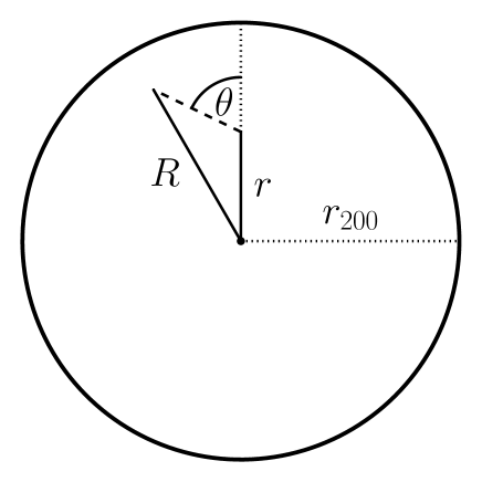
Figure 1: The coordinate system used to calculate the angular dependence of the column density of each species at a given radial coordinate (see Eq. 12 and Eq. 13).

We assume that the distributions of gas and dark matter are spherically symmetric. Under this assumption, gas at a distance $r$ from the centre of a dark matter halo is irradiated by background photons from all directions. The radiation field is therefore attenuated by a different amount depending on the density distribution of the gas along a given direction. If $J_{0}(\nu)$ represents the unattenuated radiation field at a frequency $\nu$, and $2\pi\sin(\theta){\rm d}\theta/4\pi$ is the fraction of sky with an optical depth $\tau(\nu,r,\theta)$, then the intensity of the radiation field at a distance $r$ from the centre of the cloud is given by

$$J(\nu,r) = J_{0}(\nu)\int_{0}^{\pi}\!\frac{2\pi\sin(\theta)}{4\pi}\exp[-\tau(\nu,r,\theta)]{\rm d}\theta$$ (9)

$$= \frac{1}{2}\,J_{0}(\nu)\int_{-1}^{+1}\!\exp[-\tau(\nu,r,\mu)]{\rm d}\mu$$ (10)

$$\tau(\nu,r,\mu) = \sum\limits_{i}\sigma_{i}(\nu)N_{i}(r,\mu)$$ (11)

where $\mu=\cos\theta$, and $i$ corresponds to every element/ion stage that we consider in this work. Unfortunately, our calculations are computationally too demanding to include every ionization stage for all elements with atomic number $<30$ (unlike Cloudy). We have therefore incorporated only a handful of the most abundant metals that are commonly observed in metal-poor DLAs, including H i, D i, He i, He ii, C i–C iv, N i–N iv, O i–O iv, Mg i–Mg iv, Si i–Si iv. We have adopted the photoionization cross-section, $\sigma_{i}(\nu)$, of each element using the compilation by Verner et al. (1996).

At a distance $r$ from the centre of the halo, the column density of species $i$ in the direction $\theta$ can be calculated by integrating the volume density of species $i$, $n_{i}(R)$, from a radial distance $r$ to the virial radius (i.e. integrate along the path defined by the dashed line in Fig. 1):

$$N_{i}(r,\mu) = \int\limits_{r}^{r_{200}}\!\frac{R\,n_{i}(R)\,{\rm d}R}{\sqrt{R^{2}-r^{2}(1-\mu^{2})}}$$ (12)

$$N_{i}(r,\mu) = \!\!\!\!\!\!\!\int\limits_{r\sqrt{1-\mu^{2}}}^{r}\!\!\!\!\!\frac{R\,n_{i}(R)\,{\rm d}R}{\sqrt{R^{2}-r^{2}(1-\mu^{2})}}+\!\!\!\!\!\!\!\int\limits_{r\sqrt{1-\mu^{2}}}^{r_{200}}\!\!\!\!\!\frac{R\,n_{i}(R)\,{\rm d}R}{\sqrt{R^{2}-r^{2}(1-\mu^{2})}}$$ (13)

where Eq. 12 is used for $0\leq\theta\leq\pi/2$ and Eq. 13 is used for $\pi/2<\theta\leq\pi$. The rate of primary ionizing photons at a given radius from the cloud centre of each species is then

$$\Gamma_{\rm p}(r)=4\pi\int_{\nu_{i}}^{\infty}\!\frac{J(\nu,r)}{h\nu}\sigma_{i}(\nu){\rm d}\nu$$ (14)

where $h\nu_{i}$ is the ionization energy of ion $i$. Each radiation field considered in this work is finely interpolated around the ionization energy of each ion to ensure numerical accuracy in the integrations.

The rate of collisional ionization, $\Gamma_{\rm ci}(T)$, is incorporated in our models using the Dere (2007) rate calculations. Photoionization of H i, He i, and He ii from recombinations of these species, $\Gamma_{\rm r}$, is included using equations B1, B2, B3, B6, and B7 from Jenkins (2013). We have also included the contribution from secondary collisional ionizations from energetic primary photoelectrons, $\Gamma_{\rm s}$, using the prescription outlined in Ricotti, Gnedin, & Shull (2002, cf. ). The sum of these four ionization rates for each element and ion stage is denoted $\Gamma({\rm X}^{\rm q+})$ at each radial position. Radiative and dielectronic recombination rates, $\alpha_{\rm r}(T)$, are calculated using the method outlined by Badnell et al. (2003) and Badnell (2006). Finally, rates for charge exchange ionization and recombination are determined using the Kingdon & Ferland (1996) database. We define the charge transfer coefficients for reactions of ion ${\rm X}^{\rm q+}$ with H or He using the characters $C$ or $D$ respectively, according to the following definitions:

$$C_{\rm i}({\rm X}^{\rm q+},T) = {\rm X}^{\rm q+}+{\rm H}^{+}\to{\rm X}^{\rm(q+1)+}+{\rm H}^{0}$$ (15)

$$C_{\rm r}({\rm X}^{\rm q+},T) = {\rm X}^{\rm q+}+{\rm H}^{0}\to{\rm X}^{\rm(q-1)+}+{\rm H}^{+}$$ (16)

$$D_{\rm i}({\rm X}^{\rm q+},T) = {\rm X}^{\rm q+}+{\rm He}^{+}\to{\rm X}^{\rm(q+1)+}+{\rm He}^{0}$$ (17)

$$D_{\rm r}({\rm X}^{\rm q+},T) = {\rm X}^{\rm q+}+{\rm He}^{0}\to{\rm X}^{\rm(q-1)+}+{\rm He}^{+}$$ (18)

The rates for charge exchange between deuterium and hydrogen were derived from the data listed in Table 1 of Savin (2002). As we discuss in Section 4, the relative reaction rate for deuterium charge exchange ionization and recombination largely determines the deuterium ionization correction. Since the ionization potential for H is less than D, the rate of the endothermic reaction $C_{\rm i}({\rm D}^{\rm 0},T)$ should always be less than that of the exothermic reaction $C_{\rm r}({\rm D}^{\rm+},T)$. We note that the approximate fitting formulae provided by Savin (2002) reverse the endothermic and exothermic nature of the reaction in the temperature range 4,500 K – 100,000 K (i.e. $C_{\rm i}({\rm D}^{\rm 0},T)$ is larger than $C_{\rm r}({\rm D}^{\rm+},T)$). This approximation leads to a notable and incorrect change to both the magnitude and sign of the deuterium ionization correction. We therefore adopt their recommended fitting function for deuterium charge exchange ionization:

$$C_{\rm i}({\rm D}^{\rm 0},T)=2\times 10^{-10}\,T^{0.402}\,\exp\,(-37.1/T)\,-\,3.31\times 10^{-17}\,T^{1.48}$$ (19)

and adopt the following form for deuterium charge exchange recombination, under the assumption of chemical equilibrium:

$$C_{\rm r}({\rm D}^{\rm+},T)=C_{\rm i}({\rm D}^{\rm 0},T)\times\exp\,(42.915/T)$$ (20)

where $42.915\,{\rm K}$ is the difference in ionization potential of D relative to H. Eq. 20 provides an accurate description of the relative reaction rate data (to within 0.6 per cent) compiled by Savin (2002) in the temperature range 2 K – 200,000 K, and ensures that $C_{\rm i}({\rm D}^{\rm 0},T)$ is always less than $C_{\rm r}({\rm D}^{\rm+},T)$.

Throughout this work, we assume that each element is in ionization equilibrium, such that:

$$\big{[}\Gamma({\rm X}^{\rm q+})+C_{\rm i}({\rm X}^{\rm q+},T)\,n({\rm H}^{+})+D_{\rm i}({\rm X}^{\rm q+},T)\,n({\rm He}^{+})\big{]}\,n({\rm X}^{\rm q+})=$$

$$\big{[}\alpha_{\rm r}({\rm X}^{\rm q+},T)\,n_{\rm e}+C_{\rm r}({\rm X}^{\rm(q+1)+},T)\,n({\rm H}^{0})+D_{\rm r}({\rm X}^{\rm(q+1)+},T)\,n({\rm He}^{0})\big{]}\times$$

$$\,n({\rm X}^{\rm(q+1)+})$$ (21)

for the q ionization states of a given element X. The electron density, $n_{\rm e}$, is calculated from H and He ionizations, and we ignore the contribution of electrons from the ionization of metals. Considering all ionization states for a given element, Eq. 2.3 represents a set of simultaneous equations that can be solved for the fractional ionization of a given species at each radial coordinate, ${\cal F_{\rm X^{q+}}}\equiv n({\rm X^{q+}})/n({\rm X})$.

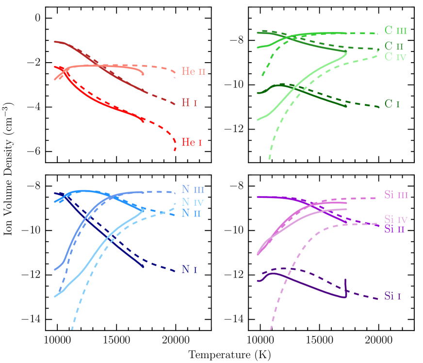
Figure 2: The temperature-density relation for a plane parallel slab of constant density gas. The dashed lines indicate the results from our model calculations, while the solid lines were calculated using the Cloudy photoionization software. In general, there is a good agreement between the two codes.

2.4 Thermal Equilibrium

In addition to ionization equilibrium, we assume that the gas is in thermal equilibrium such that the total heating rate exactly balances the total cooling rate at each radial coordinate. The heating rate includes contributions from both photoionization heating and secondary heating by primary photoelectrons. The photoionization heating rate for each chemical element at a given radius is given by:

$${\cal H}({\rm X}^{\rm q+})=n({\rm X}^{\rm q+})\int\limits_{\nu_{\rm i}}^{\infty}\!\sigma_{\rm i}(\nu)~{}J(\nu,r)~{}\frac{h\nu-h\nu_{\rm i}}{h\nu}~{}{\rm d}\nu$$ (22)

and the total heating rate is summed over all species. The cooling rate includes contributions from collisional excitation/ionization cooling, single electron and dielectronic recombination cooling, Bremsstrahlung cooling and Compton heating/cooling (see equations 12a-17 from Cen (1992) for a complete list of the adopted cooling formulae). Given the very low metallicity of the gas being probed (typically $<1/100$ solar), we have ignored metal cooling in our calculation, and do not expect this to considerably alter our conclusions.

2.5 Numerical Method

Our calculations are qualitatively similar to those presented by Kepner, Babul, & Spergel (1997) and Sternberg, McKee, & Wolfire (2002). We use an iterative procedure to solve the equations of thermal and ionization equilibrium. Each model calculation is initialised with a primordial ⁴He mass fraction ${\rm Y}_{\rm P}=0.25$, and a primordial deuterium abundance $\log\,({\rm D/H})_{\rm P}=-4.60$. We assume that the model DLAs have a metal abundance distribution that is consistent with the solar abundance pattern, scaled to a metallicity $1/1000$ solar. We then select a dark matter halo mass ($M_{200}$), and a scaling factor ($f_{200}$) to determine the total mass of baryons within the halo virial radius. The initial gas temperature is set to 20,000 K, and we assume that the gas is mostly ionized. As we discuss in Section 4, the most important factor in determining the magnitude of the D/H ionization correction is D$\leftrightarrow$H charge exchange, which does not depend on any of the above assumptions.

These initial parameter values allow us to numerically solve the integral in Eq. 7, and determine the pressure profile of the gas. Using Eq. 2.2, we can then calculate the gas density profile. The gas density profile establishes the radiation field at a given radial coordinate (Eq. 9-13). We then solve for ionization equilibrium to calculate the fractional ionization of each species, ${\cal F_{\rm X^{q+}}}$, at all radial coordinates. To increase the efficiency of our computation, we sub-iterate over the solution to the equations of ionization balance, holding the temperature and radiation field constant at each coordinate, until the relative difference of ${\cal F_{\rm X^{q+}}}$ between each sub-iteration for all species is less than $10^{-5}$.

The photoheating rate at each radial position is calculated using the values of $n({\rm X}^{\rm q+})$ determined from ${\cal F_{\rm X^{q+}}}$ and the corresponding radiation field at this position. We then estimate the temperature profile of the gas assuming thermal equilibrium. With this new temperature profile, we recalculate the integral in Eq. 7 for the pressure profile. We then iterate the procedure described above until the relative difference of ${\cal F_{\rm X^{q+}}}$ between successive iterations for all species is less than $10^{-5}$.

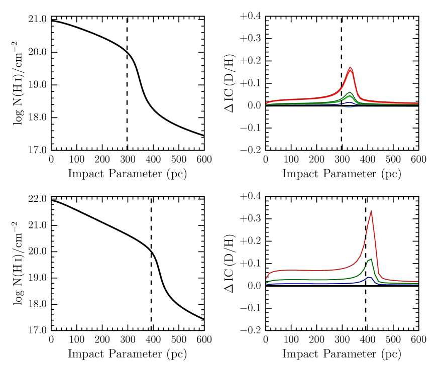
Figure 3: We performed a convergence test on two model halos to optimise the computational speed and accuracy of our calculations. The results presented in the top panels correspond to a $10^{8.4}~{}{\rm M}_{\odot}$ dark matter halo with a baryon fraction $f_{200}=1.0$ (i.e. the Universal baryon fraction), and the bottom panels present the results for a $10^{8.9}~{}{\rm M}_{\odot}$ dark matter halo with $f_{200}=0.3$. Both calculations were performed at redshift $z=3$, with an isotropic, Haardt & Madau (2012) incident radiation field. The solid black lines in the left panels display the H i column density profile of the halo. In the right panels, we illustrate the fractional change of the deuterium ionization correction between a high resolution calculation (solid black line), and various lower resolution calculations (see Eq. 24 and text for further details); the red, green, and blue curves correspond to a radial sampling, $n_{\rm r}$ = 500, 1000, and 2000 respectively. Light to dark shades of each coloured curve (almost indistinguishable over the plotted radial range) correspond to an angular sampling $n_{\mu}$ = 30, 90, and 180, respectively. The vertical dashed line in all panels corresponds to the radius where the H i column density $N({\rm H\,\textsc{i}})=10^{20}~{}{\rm cm}^{-2}$. Note that $\Delta$IC(D/H) represents the fractional change in the deuterium ionization correction (i.e. $+0.1\equiv 10$ per cent uncertainty in the value of the correction; see Eq. 24).

2.6 Model Observables

In general, information on metal-poor DLAs is restricted to a single line-of-sight to a background quasar. For a quasar that intersects a metal-poor DLA at an impact parameter $b$, with respect to the centre of the dark matter halo, the measured column density of the species X^q+ is given by

$$N_{\rm X^{\rm q+}}(b)=2\int\limits_{b}^{\infty}\!\frac{r}{\sqrt{r^{2}-b^{2}}}\,n({\rm X^{\rm q+}},r)\,{\rm d}r$$ (23)

2.7 Numerical Stability and Convergence

2.7.1 Stability

We performed a series of checks to ensure the reliability of our code. We first tested the implementation of our ionization and thermal equilibrium equations by modelling a plane parallel slab of constant density gas ($n({\rm H})=0.1~{}{\rm cm}^{-3}$) illuminated on one side by a power law radiation field ($f(\nu)\propto\nu^{\alpha}$) with index $\alpha=-1$. Our simulation was stopped once a neutral H column density of $10^{20.3}$ H i atoms cm^-2 was reached. These parameters correspond to a typical DLA, irradiated on one side by a quasar. The relationships between temperature and density for each chemical species in our calculations are shown by the dashed curves in Fig. 2. We have performed a nearly identical calculation with the Cloudy photoionization software (Ferland et al., 2013). The results from the Cloudy simulation are shown as solid lines in Fig. 2.

There is a good agreement between the two codes for all ion stages of the most abundant elements, including H, He, C, and N (as well as O, not shown). The primary disagreement between Cloudy and our code for these elements is seen for the high ionization stages at low temperatures. This difference is due to the large number of physical processes that are included in Cloudy, but are not present in our code. The most important temperature regime to correctly model corresponds to where the ion density is most abundant, since this regime tends to be the dominant contribution to the column density. For these elements, our code produces acceptable results. The temperature-density relationships for the Si ions (as well as Mg, not shown), on the other hand, show a higher level of disagreement between the two codes, particularly for the higher ion stages. This discrepancy is likely due to the exclusion of elements with a similar abundance to Si (e.g. Ne, Fe), as well as the exclusion of several physical processes included in Cloudy (discussed above) and small differences between the heating and cooling functions used by the two codes. We note, however, that there is an acceptable agreement between the two codes for the ions of interest to our study (including H i, C ii, C iii, N i, N ii, Si ii and Si iii). Specifically, the difference between our code and Cloudy for the column density ratio of successive ion stages are:

$$\log~{}N(\mathrm{C\,\textsc{iii})/N(C\,\textsc{ii}})_{\rm our~{}code}~{}-~{}\log~{}N(\mathrm{C\,\textsc{iii})/N(C\,\textsc{ii}})_{\rm cloudy}=-0.09$$

$$\log~{}N(\mathrm{N\,\textsc{ii})/N(N\,\textsc{i}})_{\rm our~{}code}~{}-~{}\log~{}N(\mathrm{N\,\textsc{ii})/N(N\,\textsc{i}})_{\rm cloudy}=+0.02$$

$$\log~{}N(\mathrm{Si\,\textsc{iii})/N(Si\,\textsc{ii}})_{\rm our~{}code}~{}-~{}\log~{}N(\mathrm{Si\,\textsc{iii})/N(Si\,\textsc{ii}})_{\rm cloudy}=+0.40$$

Therefore, as discussed above, we conclude that the Si ratio shows the highest level of disagreement between the two codes.

2.7.2 Convergence

We then performed a convergence and optimisation study, to determine the number of radial coordinates needed to accurately evaluate the numerical integrations over radius and $\cos\theta$ for the NFW geometry. We conducted two simulations: (1) A $10^{8.4}~{}{\rm M}_{\odot}$ dark matter halo with $f_{200}=1.0$ (top panels of Fig. 3); and (2) a $10^{8.9}~{}{\rm M}_{\odot}$ dark matter halo with $f_{200}=0.3$ (bottom panels of Fig. 3). Both calculations assume that the halo is exposed to an isotropic Haardt & Madau (2012) background radiation field at redshift $z=3$. The former and latter halos produce a maximum neutral hydrogen column density of $N({\rm H\,\textsc{i}})\simeq 10^{21}~{}{\rm cm}^{-2}$ and $N({\rm H\,\textsc{i}})\simeq 10^{22}~{}{\rm cm}^{-2}$ respectively, for a line-of-sight that passes directly through the centre of the halo (corresponding to $b=0$ in Eq. 23). The H i column density profiles as a function of impact parameter for these two halos are shown in the left panels of Fig. 3, where the vertical dashed line corresponds to the radius where $N({\rm H\,\textsc{i}})=10^{20}~{}{\rm cm}^{-2}$.

We began the simulations with a very fine sampling of $n_{\mu}=720$ angular coordinates over $\cos\theta$, and $n_{\rm r}=5000$ radial coordinates linearly spaced between the centre of the halo and $r_{200}$. We then explored various combinations of these samplings to optimise the efficiency of our calculations whilst maintaining numerical accuracy. Our grid spanned $n_{\mu}~{}=~{}[30,90,180]$ and $n_{\rm r}~{}=~{}[500,1000,2000]$. The right panels of Fig. 3 illustrate the results of our convergence study, where $\Delta{\rm IC(D/H})$ is the fractional change to the ionization correction for different choices of the numerical integration parameters:

$$\Delta{\rm IC(D/H})\equiv\frac{{\rm IC(D/H})_{\rm 720,5000}-{\rm IC(D/H})_{n_{\mu},n_{\rm r}}}{{\rm IC(D/H})_{720,5000}}$$ (24)

where IC(D/H) is defined below, in Eq. 25. As expected, the choice of $n_{\rm r}$ is most sensitive to the region where the neutral gas is becoming more ionized, somewhat below the classical DLA threshold of $N({\rm H\,\textsc{i}})=10^{20.3}~{}{\rm cm}^{-2}$. On the other hand, the choice of $n_{\rm\mu}$ only becomes important when $r~{}\gg~{}r_{\rm DLA}$, well beyond the radial regime of interest to this study. The optimal combination for our study is therefore $n_{\mu}=30$ angular coordinates and $n_{\rm r}=1000$ radial coordinates, which provided a deuterium ionization correction that is accurate to within $\sim 10$ per cent when $N({\rm H\,\textsc{i}})\geq 10^{20}~{}{\rm cm}^{-2}$.

3 D/H Ionization Correction

We now discuss the results from our calculations to determine the deuterium ionization correction. In what follows, we define the true value of the D/H abundance to be

$$\log_{10}{\rm D/H}=\log_{10}N({\rm D}\,\textrm{{\sc i}})/N({\rm H}\,\textrm{{\sc i}})+{\rm IC(D/H)}$$ (25)

where ${\rm IC(D/H)}$ is the deuterium ionization correction derived from our model calculations. We adopt a typical value for the ‘true’ deuterium abundance, $\log_{10}{\rm D/H}=-4.60$. We have computed a series of calculations with a simple plane parallel geometry as well as a more ‘realistic’ geometry where the gas is confined to an NFW halo.

3.1 Plane Parallel Models

The simplest geometry to consider is a uniform, plane parallel, constant volume density slab of gas, illuminated on one side. For our calculations, we have assumed the gas slab is irradiated by the Haardt & Madau (2012) radiation field at redshift $z=3$, incident normal to the surface of the slab. We computed a grid of calculations covering a range in H volume density ($-2.0\leq\log\,n_{\rm H}/{\rm cm}^{-3}\leq 2.0$, in steps of 0.5 dex) and H i column density ($19.0\leq\log\,N({\rm H\,\textsc{i}})/{\rm cm}^{-2}\leq 21.0$, in steps of 0.5 dex). The metals were assumed to be in solar relative proportion (Asplund et al., 2009), and globally scaled to a metallicity of $1/1000~{}Z_{\odot}$. The depth of the slab was increased until the desired H i column density had been reached. The depth of each simulated slab was sampled linearly by 1000 values. Note that changing the H volume density is equivalent to changing the intensity (but not the shape) of the incident radiation field.

The results of our calculations are presented in the left panel of Fig. 4, where the red, green and blue curves correspond to the column density ratios $N({\rm C\,\textsc{iii}})/N({\rm C\,\textsc{ii}})$, $N({\rm N\,\textsc{ii}})/N({\rm N\,\textsc{i}})$, and $N({\rm Si\,\textsc{iii}})/N({\rm Si\,\textsc{ii}})$ respectively. In all cases, the ionization correction for deuterium is negative for the set of H volume densities and H i column densities considered in this work. The maximum correction in our models is $-0.0015$ dex (i.e. $\sim 0.4$ per cent), corresponding to gas with a low H i column density ($N$(H i)$<10^{20}~{}{\rm cm}^{-2}$) and/or high ionization. ${\rm IC(D/H)}$ exhibits a similar dependence on the C and Si ion ratios. The deuterium ionization correction for these ions depends on the values of the ion ratio and the H i column density. On the other hand, the deuterium ionization correction determined from the N ion ratio is almost independent of the H i column density. For the range of $n_{\rm H}$ and $N$(H i) considered here, the following fitting formula can be used to estimate the ionization correction:

$$e^{{\rm IC(D/H)}}=-\sum_{m}\sum_{n}a_{nm}~{}(\log_{10}N(\textrm{H\,{\sc i}})/{\rm cm}^{-2})^{n}~{}(\log_{10}{\rm IR})^{m}$$ (26)

where IR corresponds to the column density ratio of successive ion stages (for example, IR=$N({\rm C\,\textsc{iii}})/N({\rm C\,\textsc{ii}})$, $N({\rm N\,\textsc{ii}})/N({\rm N\,\textsc{i}})$, or $N({\rm Si\,\textsc{iii}})/N({\rm Si\,\textsc{ii}})$), and the $a_{nm}$ coefficients are provided in Table 1. We caution against extrapolating these curves beyond the appropriate ranges shown in the left panel of Fig. 4.

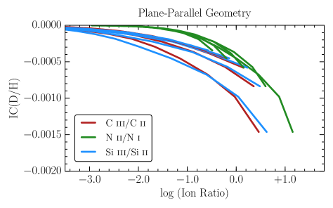
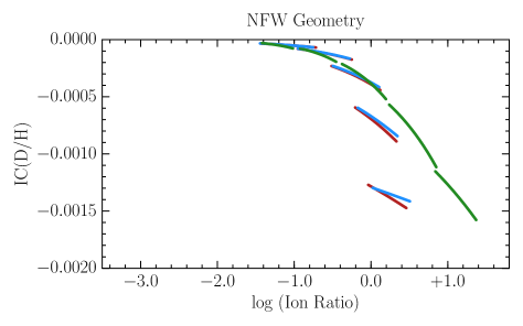
Figure 4: The deuterium ionization correction is shown for a gas cloud exposed to the Haardt & Madau (2012) background radiation field. The left panel illustrates the results for a plane parallel geometry with uniform volume density, while the right panel illustrates the correction for a gas cloud in hydrostatic equilibrium with an NFW potential. The red, green and blue curves illustrate how the D/H ionization correction depends on the C iii/C ii, N ii/N i, and Si iii/Si ii ion ratios. Each curve represents the correction at a given H i column density. There are 5 curves for each ion ratio, corresponding to H i column densities log $N$(H i)/cm${}^{-2}=19.0,19.5,20.0,20.5,{\rm and}\,21.0$. In the case of N ii/N i, the curves for different values of $N$(H i) largely overlap with one another. For each ion ratio, the curve with the most negative IC(D/H) values corresponds to a log $N$(H i)/cm${}^{-2}=19.0$; IC(D/H) becomes smaller as the H i column density increases. The curves in the left panel cover a range in H volume density ($-2.0\leq\log\,n_{\rm H}/{\rm cm}^{-3}\leq 2.0$), while the curves in the right panel consider a range in the physical properties of an NFW halo (e.g. halo mass, baryon fraction, radiation intensity; see text for further details).

Table 1: plane-parallel ionization correction coefficients

C iii/C ii
$n$	$m$
	$0$	$1$	$2$	$3$
$0$	$114.39$	$25.084$	$17.063$	$2.8237$
$1$	$-11.816$	$-2.3171$	$-1.6591$	$-0.2769$
$2$	$0.2860$	$0.05441$	$0.03993$	$0.00675$
N ii/N i
$n$	$m$
	$0$	$1$	$2$	$3$
$0$	$144.62$	$83.202$	$26.766$	$9.9952$
$1$	$-15.688$	$-8.8214$	$-2.8651$	$-0.98627$
$2$	$0.40361$	$0.23679$	$0.07629$	$0.0244$
Si iii/Si ii
$n$	$m$
	$0$	$1$	$2$	$3$
$0$	$148.77$	$48.975$	$17.508$	$2.9050$
$1$	$-15.372$	$-4.9716$	$-1.7676$	$-0.2844$
$2$	$0.3777$	$0.1277$	$0.04468$	$0.00701$

3.2 NFW Models

As shown in Section 3.1, the D/H ionization correction could become comparable to the measurement precision in the near future. It is therefore necessary to test if the ionization correction depends on the geometry of the gas. In this section, we explore a gas geometry that might represent more closely the physical state of the gas that gives rise to metal-poor DLAs, rather than a simple gas slab of uniform density. In what follows, we discuss the results from modelling metal-poor DLAs as gas in hydrostatic pressure equilibrium with the potential of a host NFW dark matter halo.

For a metal-poor DLA that is probed by the sightline to a background quasar, there are several unknown physical properties that cannot be determined directly. These include: (1) The host dark matter halo mass, $M_{200}$, of the DLA; (2) The baryon fraction, $f_{200}$, of the halo; (3) The intensity of the incident radiation field; and (4) The shape of the radiation field. Other properties, such as the redshift, turbulent Doppler parameter, and metal abundances of the DLA can be inferred from observations. We adopt typical parameter values for these quantities: $z=3$, $b_{\rm turb}=3.0~{}{\rm km~{}s}^{-1}$, and we globally scale the metals to 1/1000 $Z_{\odot}$, in solar relative proportions. To reduce the computational demand of these calculations, we only consider the Haardt & Madau (2012) radiation field shape at the appropriate redshift, and scale the intensity by a factor of either $1/3$, $1$, or $3$. As we discuss in Section 4, changing the shape of the radiation field does not effect the estimated deuterium ionization correction. We consider models that have a baryon fraction in the range $\log_{10}~{}f_{200}=-1.0,-0.5$ and 0.0. Each numerical grid was sampled with $n_{\rm r}$ = 1000 radial coordinates, and $n_{\mu}$ = 30 angular coordinates, as discussed in Section 2.7.2.

Table 2: NFW ionization correction coefficients

C iii/C ii
$n$	$m$
	$0$	$1$
$0$	$48.26$	$-156.23$
$1$	$-4.5054$	$15.377$
$2$	$0.0850$	$-0.37572$
N ii/N i
$n$	$m$
	$0$	$1$
$0$	$262.58$	$-55.013$
$1$	$-27.121$	$4.7885$
$2$	$0.67994$	$-0.0980$
Si iii/Si ii
$n$	$m$
	$0$	$1$
$0$	$74.500$	$-155.98$
$1$	$-7.1525$	$15.266$
$2$	$0.15165$	$-0.3709$

We began our calculations with a halo mass $\log_{10}M_{200}/M_{\odot}=7.0$, for each grid value of the radiation intensity and $f_{200}$. As discussed in Section 2.5, the first iteration of our numerical solution was initialised with a gas temperature of 20,000 K, and the gas was assumed to be mostly ionized. No dark matter halo with $\log_{10}M_{200}/M_{\odot}=7.0$ was able to host gas that would appear as a DLA at $z\sim 3$. We then increased the virial mass of each halo by $0.1~{}{\rm dex}$, using as input the final thermal and ionization structure that were output by the previous model. By initialising the simulations with the solution from the previous model, the computational requirement was greatly reduced. We sequentially increased the dark matter halo mass until the peak $N$(H i) of a halo had exceeded $\sim 10^{21.5}~{}{\rm cm}^{-2}$. At these H i column densities, molecular H formation (and presumably star formation) is an important factor to consider (Noterdaeme, Petitjean, & Srianand, 2015), and is not included in our modelling procedure.

Our final model suite comprises all sightlines through these dark matter halos that produce an H i column density in excess of $10^{19}~{}{\rm cm}^{-2}$. In the right panel of Fig. 4 we show the results of our NFW calculations, which are qualitatively similar to the plane parallel geometry; the D/H ionization correction is most sensitive to the column density ratio of the successive stages of metal ionization (and to a lesser extent on the H i column density). However, the ionization correction in the NFW geometry also depends on the grid of parameter values (halo mass, $f_{200}$, etc.), which introduce an uncertainty in this correction. The N ion ratio provides the most reliable correction, accurate to within $2\times 10^{-5}$ dex (6 per cent) for log $N$(H i)/cm${}^{-2}>20.0$ over the entire grid of parameter space considered here. The uncertainty is considerably worse for the C and Si ion ratios, which have a 30 per cent uncertainty in the correction over the entire range (i.e. a correction uncertainty of up to $1\times 10^{-4}$ dex when the ion ratio is near unity). For each of these ion ratios we provide fitting formulae for the ionization correction factors, in the form of Eq. 28, with the $a_{nm}$ coefficients listed in Table 2. These calculations represent the central values of the ionization correction, and should be used together with the percentage uncertainties quoted above.

4 Discussion

Our calculations with both geometries suggest that deuterium is slightly underionized relative to hydrogen in metal-poor DLAs. By disabling the individual physical processes in our code, we conclude that the dominant physical process that sets the deuterium ionization correction is D $\leftrightarrow$ H charge transfer; specifically, the negative ionization correction term is the result of the preferred (exothermic) charge transfer recombination reaction D⁺ + H${}^{0}~{}\to~{}$D⁰ + H⁺. Photoionization plays a minimal role; thus, the most important factor to determine the deuterium ionization correction in DLAs and sub-DLAs is the H volume density and the gas temperature, not the incident radiation field.

There are a few remarkable similarities and differences between the two geometries considered in this paper. The first major difference between the NFW and plane parallel models is the spread of ion ratios for a given H i column density; the NFW models exhibit a very small range in the ion ratios (typically $0.5$ dex), whereas the plane parallel models cover a much larger range (at least $5$ dex). This difference is purely a geometrical effect, since the gas density profile in the NFW geometry is more limited, yet has the advantage of being more physically motivated. Another difference between the two geometries is the value of the deuterium ionization correction using the C and Si ion ratios. The plane parallel models underpredict the ionization correction for H i column densities $\lesssim 10^{20}$ cm^-2, and overpredict the correction when $N$(H i) $\gtrsim 10^{20}$ cm^-2. The N ii/N i ion ratio, on the other hand, is nearly identical regardless of the gas geometry, and therefore offers the least geometry dependent correction.

The invariance of the N ii/N i ratio with geometry or any of the parameter space that we have explored is because the charge transfer recombination reaction N⁺ + H${}^{0}~{}\to~{}$N⁰ + H⁺ sets the N ii/N i ratio when log $N$(H i)/${\rm cm}^{-2}\gtrsim 19.5$. Therefore, $N$(N ii)/$N$(N i) $\propto$ $N$(D ii)/$N$(D i) $\propto$ $N$(H ii)/$N$(H i) for large H i column densities. On the other hand, when log $N$(H i)/${\rm cm}^{-2}\lesssim 19.5$, primary photoionization drives the determination of the N ii/N i ratio. We therefore conclude that the most suitable systems for measuring the primordial deuterium abundance are those with log $N$(H i)/${\rm cm}^{-2}\gtrsim 20.0$ for the following reasons: (1) The deuterium ionization correction factor is relatively small (typically $\lesssim 0.0005$ dex); (2) If an ionization correction needs to be applied in the future, the N ii/N i ratio should depend only on charge exchange, similarly for the D ii/D i ratio, and should be largely independent of the unknown physical properties of the system (e.g. density, shape/intensity of the incident radiation field); and (3) As discussed in Cooke et al. (2014), the Lorentzian damping wings of the H i Ly$\alpha$ absorption line, together with the multitude of weak high order Lyman series D i absorption lines, offer an determination of the $N$(D i) / $N$(H i) ratio that is largely independent of the cloud model.

Under the assumption that D $\leftrightarrow$ H charge transfer is the dominant process that sets the D/H ionization correction, we can combine Eq. 20 and Eq. 2.3 to obtain the following relation:

$$n({\rm D}^{0})=\frac{n({\rm H}^{0})\,n({\rm H})\,10^{\rm(D/H)_{\rm P}}}{n({\rm H}^{0})+n({\rm H}^{+})\exp(-42.915/T)}$$ (27)

where $({\rm D/H})_{\rm P}=-4.60$ is the assumed primordial abundance of deuterium. Eq. 27 can be applied in post-processing to more detailed photoionization calculations, such as Cloudy, that include a much larger range of physical processes than our calculations. Since N ii/N i is independent of geometry, the relationship between N ii/N i and IC(D/H) using the Cloudy photoionization software and Eq. 27 should offer the most reliable ionization correction. We therefore conclude that the following simple relation should be used to estimate the deuterium ionization correction factor:

$${\rm IC(D/H)}=-\exp(-8.2+1.2\,{\rm IR})$$ (28)

where IR $=\log_{10}N({\rm N\,\textsc{ii}})/N({\rm N\,\textsc{i}})$ and, as discussed in Section 3.2, IC(D/H) should be used with a $2\times 10^{-5}$ dex (i.e. 6 per cent) uncertainty in the ionization correction factor.

Although the deuterium ionization correction estimated herein does not significantly alter the current determination of the primordial deuterium abundance, it will become important to consider this systematic offset in the near-future. We propose that the N ii/N i ratio provides the most robust ionization correction for deuterium, since it is insensitive to the various known and unknown physical properties of metal-poor DLAs (e.g. cloud geometry, halo mass, H i column density, etc.). Unfortunately, nitrogen is notably underabundant in metal-poor DLAs (Pettini et al., 2008; Cooke et al., 2011; Pettini & Cooke, 2012b; Zafar et al., 2014); there are typically just three nitrogen atoms for every 10,000 D atoms in the most metal-poor systems. Nevertheless, measuring the N ion ratio should be a goal for future high precision surveys that aim to accurately measure the primordial abundance of deuterium in the most metal-poor DLAs.

5 Summary and Conclusions

The $N$(D i) / $N$(H i) column density ratio that is measured using quasar absorption line systems is generally assumed to be equal to the deuterium abundance (D/H). We have tested this assumption by developing a software package that calculates the relative ionization of deuterium, hydrogen, and a selection of the most abundant metal ions. Our computations are similar in spirit to the commonly used photoionization software Cloudy. The main advantage of our code, aside from including the atomic data for deuterium, is that we are able to model the density, thermal, and ionization profile of gas held in hydrostatic equilibrium with an NFW dark matter potential. On the basis of our calculations, we draw the following conclusions:

(i) For the simple case of a uniform density, plane parallel slab of gas with similar properties to DLAs, we have confirmed that our code produces comparable results as Cloudy for the ions that are used in our work.

(ii) We performed a suite of calculations using a plane parallel geometry to estimate the correction that must be applied to the measured column density ratio $N$(D i)/$N$(H i) to determine the D/H abundance. This correction is most sensitive to the relative column densities of successive stages of metal ionization and, to a lesser degree, the total H i column density.

(iii) We also calculated the deuterium ionization correction for a more realistic gas density distribution, whereby a gas cloud is confined to the potential of an NFW dark matter halo irradiated by the Haardt & Madau (2012) background. For both the plane parallel and NFW geometry, we provide fitting functions to estimate the deuterium ionization correction using either the C iii/C ii, N ii/N i, or Si iii/Si ii ion ratios and the H i column density.

(iv) The relationship between the N ii/N i ion ratio and the deuterium ionization correction is remarkable. This relationship is essentially independent of all other physical properties of our model, and provides the most accurate and reliable deuterium ionization correction. The C iii/C ii and Si iii/Si ii ion ratios, although more observationally accessible, are more dependent on both the physical conditions and the geometry of the gas.

(v) We propose that systems with log $N$(H i)/${\rm cm}^{-2}\gtrsim 20.0$ are the most suitable systems to measure the primordial D/H ratio. In this H i column density regime, charge exchange ensures that $N$(N ii)/$N$(N i) $\propto$ $N$(D ii)/$N$(D i) $\propto$ $N$(H ii)/$N$(H i), allowing a reliable ionization correction factor to be determined.

(vi) Our work provides the first quantitative analysis of the deuterium ionization correction in metal-poor DLAs, and confirms the qualitative conclusions drawn by Savin (2002): The deuterium ionization correction can be safely neglected when the D i/H i abundance ratio is measured in a DLA that is in thermal and ionization equilibrium.

The deuterium ionization correction for a typical system in the recent analysis by Cooke et al. (2014) is likely to be $\lesssim 0.1$ per cent, which is well below the current measurement uncertainty (2 per cent); the ionization correction is therefore not an important consideration at present. However, new cases of metal-poor DLAs that exhibit clean D i absorption lines are being identified, and the search for such systems will be greatly expanded with the next generation of 30+ m telescopes coming on line in the next decade. At that time, a reliable ionization correction factor for deuterium will be required, as the statistics of D/H measurements improve significantly beyond the current limited dataset.

References

- Aoki et al. (2009) Aoki W., Barklem P. S., Beers T. C., Christlieb N., Inoue S., García Pérez A. E., Norris J. E., Carollo D., 2009, ApJ, 698, 1803
- Asplund et al. (2006) Asplund M., Lambert D. L., Nissen P. E., Primas F., Smith V. V., 2006, ApJ, 644, 229
- Asplund et al. (2009) Asplund M., Grevesse N., Sauval A. J., Scott P., 2009, ARA&A, 47, 481
- Aver, Olive, & Skillman (2015) Aver E., Olive K. A., Skillman E. D., 2015, JCAP submitted, arXiv:1503.08146
- Badnell et al. (2003) Badnell N. R., et al., 2003, A&A, 406, 1151
- Badnell (2006) Badnell N. R., 2006, ApJS, 167, 334
- Cen (1992) Cen R., 1992, ApJS, 78, 341
- Cooke et al. (2011) Cooke R., Pettini M., Steidel C. C., Rudie G. C., Nissen P. E., 2011, MNRAS, 417, 1534
- Cooke, Pettini, & Murphy (2012) Cooke R., Pettini M., Murphy M. T., 2012, MNRAS, 425, 347
- Cooke et al. (2013) Cooke, R., Pettini, M., Jorgenson, R. A., et al. 2013, MNRAS, 431, 1625
- Cooke et al. (2014) Cooke R. J., Pettini M., Jorgenson R. A., Murphy M. T., Steidel C. C., 2014, ApJ, 781, 31
- Cooke, Pettini, & Jorgenson (2015) Cooke R. J., Pettini M., Jorgenson R. A., 2015, ApJ, 800, 12
- Cyburt et al. (2015) Cyburt R. H., Fields B. D., Olive K. A., Yeh T.-H., 2015, arXiv, arXiv:1505.01076
- Dekker et al. (2000) Dekker H., D’Odorico S., Kaufer A., Delabre B., Kotzlowski H., 2000, SPIE, 4008, 534
- Dere (2007) Dere K. P., 2007, A&A, 466, 771
- Ferland et al. (2013) Ferland G. J., et al., 2013, RMxAA, 49, 137
- Fields (2011) Fields B. D., 2011, ARNPS, 61, 47
- Haardt & Madau (2012) Haardt F., Madau P., 2012, ApJ, 746, 125
- Izotov, Thuan, & Guseva (2014) Izotov Y. I., Thuan T. X., Guseva N. G., 2014, MNRAS, 445, 778
- Jenkins (2013) Jenkins E. B., 2013, ApJ, 764, 25
- Kepner, Babul, & Spergel (1997) Kepner J. V., Babul A., Spergel D. N., 1997, ApJ, 487, 61
- Kingdon & Ferland (1996) Kingdon J. B., Ferland G. J., 1996, ApJS, 106, 205
- Korn et al. (2006) Korn A. J., Grundahl F., Richard O., Barklem P. S., Mashonkina L., Collet R., Piskunov N., Gustafsson B., 2006, Natur, 442, 657
- Meléndez et al. (2010) Meléndez, J., Casagrande, L., Ramírez, I., Asplund, M., & Schuster, W. J. 2010, A&A, 515, L3
- Navarro, Frenk, & White (1996) Navarro J. F., Frenk C. S., White S. D. M., 1996, ApJ, 462, 563
- Noterdaeme, Petitjean, & Srianand (2015) Noterdaeme P., Petitjean P., Srianand R., 2015, arXiv, arXiv:1505.04997
- Pettini & Cooke (2012a) Pettini M. & Cooke R., 2012a, MNRAS, 425, 2477
- Pettini & Cooke (2012b) Pettini, M., & Cooke, R. 2012b, Nuclei in the Cosmos (NIC XII), 71
- Pettini et al. (2008) Pettini M., Zych B. J., Steidel C. C., Chaffee F. H., 2008, MNRAS, 385, 2011
- Planck Collaboration et al. (2015) Planck Collaboration, et al., 2015, A&A submitted, arXiv:1502.01589
- Prada et al. (2012) Prada F., Klypin A. A., Cuesta A. J., Betancort-Rijo J. E., Primack J., 2012, MNRAS, 423, 3018
- Ricotti, Gnedin, & Shull (2002) Ricotti M., Gnedin N. Y., Shull J. M., 2002, ApJ, 575, 33
- Savin (2002) Savin D. W., 2002, ApJ, 566, 599
- Sbordone et al. (2010) Sbordone L., et al., 2010, A&A, 522, A26
- Shull & van Steenberg (1985) Shull J. M., van Steenberg M. E., 1985, ApJ, 298, 268
- Spite et al. (2015) Spite M., Spite F., Caffau E., Bonifacio P., 2015, arXiv, arXiv:1509.07809
- Sternberg, McKee, & Wolfire (2002) Sternberg A., McKee C. F., Wolfire M. G., 2002, ApJS, 143, 419
- Verner et al. (1996) Verner D. A., Ferland G. J., Korista K. T., Yakovlev D. G., 1996, ApJ, 465, 487
- Vogt et al. (1994) Vogt S. S., et al., 1994, SPIE, 2198, 362
- Zafar et al. (2014) Zafar T., Centurión M., Péroux C., Molaro P., D’Odorico V., Vladilo G., Popping A., 2014, MNRAS, 444, 744