A short survey on Lyapunov dimension for
finite dimensional dynamical systems in Euclidean space.

Abstract

Nowadays there are a number of surveys and theoretical works devoted to the Lyapunov exponents and Lyapunov dimension, however most of them are devoted to infinite dimensional systems or rely on special ergodic properties of the system. At the same time the provided illustrative examples are often finite dimensional systems and the rigorous proof of their ergodic properties can be a difficult task. Also the Lyapunov exponents and Lyapunov dimension have become so widespread and common that they are often used without references to the rigorous definitions or pioneering works.

The survey is devoted to the finite dimensional dynamical systems in Euclidean space and its aim is to explain, in a simple but rigorous way, the connection between the key works in the area: by Kaplan and Yorke (the concept of Lyapunov dimension, 1979), Douady and Oesterlé (estimation of Hausdorff dimension via the Lyapunov dimension of maps, 1980), Constantin, Eden, Foias, and Temam (estimation of Hausdorff dimension via the Lyapunov exponents and dimension of dynamical systems, 1985-90), Leonov (estimation of the Lyapunov dimension via the direct Lyapunov method, 1991), and numerical methods for the computation of Lyapunov exponents and Lyapunov dimension.

In this survey a concise overview of the classical results is presented, various definitions of Lyapunov exponents and Lyapunov dimension are discussed. An effective analytical method for the estimation of Lyapunov dimension is presented, its application to the self-excited and hidden attractors of well-known dynamical systems is demonstrated, and analytical formulas of exact Lyapunov dimension are obtained.

1 Introduction: Hausdorff dimension

The theory of topological dimension [41, 49], developed in the first half of the 20th century, is of little use in giving the scale of dimensional characteristics of attractors. The point is that the topological dimension can take integer values only. Hence the scale of dimensional characteristics compiled in this manner turns out to be quite poor. For the analysis of attractors, the Hausdorff dimension of a set is much better. This dimensional characteristic can take any nonnegative value (not greater than the topological dimension of the space), and it coincides with the topological dimension for such typical objects in Euclidean space as a smooth curve, a smooth surface, or a countable set of points.

Let us give the definition of the Hausdorff dimension and its upper estimations based on the Lyapunov exponents following mainly ([45, 27, 61, 20, 102, 31, 40, 106, 42, 10, 6, 73, 16]).

Consider a set $K\subseteq\mathbb{R}^{n}$ and numbers $d\geq 0$, $\varepsilon>0$. We cover $K$ by a countable set of balls $B_{r_{j}}$ of radius $r_{j}<\varepsilon$, and define

$$\mu_{H}(K,d,\varepsilon):=\inf\bigg{\{}\sum\limits_{j\geq 1}r_{j}^{d}|\ r_{j}\leq\varepsilon,K\subset\bigcup_{j\geq 1}B_{r_{j}}\bigg{\}},$$

where the infimum is taken over all such countable $\varepsilon$-coverings $K$. It is obvious that $\mu_{H}(K,d,\varepsilon)$ does not decrease with decreasing $\varepsilon$. Therefore there exists a limit (perhaps infinite), namely

$$\mu_{H}(K,d)=\lim\limits_{\varepsilon\to 0+0}\mu_{H}(K,d,\varepsilon)=\sup_{\varepsilon>0}\mu_{H}(K,d,\varepsilon).$$

Definition 1

The function $\mu_{H}(\cdot,d)$ is called the Hausdorff $d$-measure on $\mathbb{R}^{n}$.

For a certain set $K$, the function $\mu_{H}(K,\cdot)$ has the following property. It is possible to find $d_{cr}=d_{cr}(K)\in[0,n]$ such that

$$\begin{array}[]{l}\mu_{H}(K,d)=\infty,\ \forall d\,\in(0,d_{cr});\quad\mu_{H}(K,d)=0,\ \forall\,d>d_{cr}.\end{array}$$

We have $d_{cr}(\mathbb{R}^{n})=n$.

Definition 2

The Hausdorff dimension of the set $K$ is defined as

$$\dim_{\rm H}K:=d_{cr}(K)=\inf\{d\geq 0\mid\mu_{H}(K,d)=0\}.$$

2 Singular value function and invariant sets of maps and dynamical systems

In the seminal paper [27] Douady and Oesterlé showed how to obtain an upper estimate of the Hausdorff dimension of set $K$. To demonstrate their approach, let us consider some definitions and auxiliary results.

Let $U$ be an open subset of $\mathbb{R}^{n}$ and $\varphi:U\to\mathbb{R}^{n}$ be a continuously differentiable map. With respect to the canonical basis in $\mathbb{R}^{n}$ the function $\varphi(u)$ has the $n\times n$ Jacobian matrix

$$D\varphi(u)=D_{u}\varphi(u)=\left(\frac{\partial\varphi_{i}(u)}{\partial u_{j}}\right)_{n\times n},\quad u\in U.$$

Let $\sigma_{i}(u)=\sigma_{i}(D\varphi(u))$, $i=1,2,...,n$, be the singular values of $D\varphi(u)$ (i.e. $\sigma_{i}(u)\geq 0$ and $\sigma_{i}(u)^{2}$ are the eigenvalues of the symmetric matrix $D\varphi(u)^{*}D\varphi(u)$ with respect to their algebraic multiplicity) ordered so that $\sigma_{1}(u)\geq\cdots\geq\sigma_{n}(u)\geq 0$ for any $u\in K$. If $\sigma_{n}(u)>0$, then the unit ball $B$ is transformed by $D\varphi(u)$ into the ellipsoid $D\varphi(u)B$ and the lengths of its principal semiaxes coincide with the singular values.

Definition 3

The singular value function of $D\varphi(u)$ of order $d\in[0,n]$ at $u\in U$ is defined as

$$\omega_{d}(D\varphi(u)):=\left\{\begin{aligned} &1,&&d=0,\\ &\sigma_{1}(u)\cdots\sigma_{d}(u),&&d\in\{1,\ldots,n\},\\ &\sigma_{1}(u)\cdots\sigma_{\lfloor d\rfloor}(u)\sigma_{\lfloor d\rfloor+1}(u)^{d-\lfloor d\rfloor},&&d\in(0,1)\cup\ldots\cup(n-2,n-1),\end{aligned}\right.$$ (1)

where ${\lfloor d\rfloor}$ is the largest integer less or equal to $d$.

Remark that $|\det D\varphi(u)|=\omega_{n}(D\varphi(u))$.

Similarly, introducing the singular value function for arbitrary quadratic matrices, by the Horn inequality [39] for any two $n\times n$ matrices $A$ and $B$ and any $d\in[0,n]$ we have (see, e.g. [10, p.28])

Lemma 1

$$\omega_{d}(AC)\leq\omega_{d}(A)\omega_{d}(C).$$ (2)

Definition 4

A set $K\subset U\subseteq\mathbb{R}^{n}$ with respect to the map $\varphi$ is said to be:

1) positively invariant if $\varphi(K)\subset K,$

2) invariant if $\varphi(K)=K,$

3) and negatively invariant if $\varphi(K)\supset K,$ where $\varphi(K)=\left\{\varphi(u)~{}|~{}{u}\in K\right\}$.

Consider an autonomous differential equation

$$\dot{u}=f(u),$$ (3)

where $f:U\subseteq\mathbb{R}^{n}\to\mathbb{R}^{n}$ is a continuously differentiable vector-function. Suppose that any solution $u(t,u_{0})$ of (3) such that $u(0,u_{0})=u_{0}\in U$ exists for $t\in[0,\infty)$, is unique, and stays in $U$. Then the evolutionary operator $\varphi^{t}(u_{0}):=u(t,u_{0})$ is continuously differentiable and satisfies the semigroup property:

$$\varphi^{t+s}(u_{0})=\varphi^{t}(\varphi^{s}(u_{0})),\ \varphi^{0}(u_{0})=u_{0}\quad\forall~{}t,s\geq 0,\ \forall u_{0}\in U.$$ (4)

Thus $\{\varphi^{t}\}_{t\geq 0}$ is a smooth dynamical system in the phase space $(U,||~{}\cdot~{}||)$: $\big{(}\{\varphi^{t}\}_{t\geq 0},(U\subseteq\mathbb{R}^{n},||\cdot||)\big{)}$. Here $||u||=\sqrt{u_{1}^{2}+\cdots+u_{n}^{2}}$ is Euclidean norm of the vector ${u}=(u_{1},\ldots,u_{n})\in\mathbb{R}^{n}$. Similarly, we can consider a dynamical system generated by the difference equation

$$u(t+1)=\varphi(u(t)),\quad t=0,1,..\,,$$ (5)

where $\varphi:U\subseteq\mathbb{R}^{n}\to U$ is a continuously differentiable vector-function. Here $\varphi^{t}(u)=\underbrace{(\varphi\circ\varphi\circ\cdots\varphi)(u)}\limits_{t-{\rm times}}$, $\varphi^{0}(u)=u$, and the existence and uniqueness (in the forward-time direction) take place for all $t\geq 0$. Further $\{\varphi^{t}\}_{t\geq 0}$ denotes a smooth dynamical system with continuous or discrete time.

Definition 5

A set $K\subset U\subseteq\mathbb{R}^{n}$ with respect to the dynamical system $\{\varphi^{t}\}_{t\geq 0}$ is said to be positively invariant, invariant or negatively invariant if the corresponding property takes place with respect to the map $\varphi^{t}$ for all $t>0$.

Consider the linearizations of systems (3) and (5) along the solution $\varphi^{t}(u)$:

$$\dot{y}=J(\varphi^{t}(u))y,\quad J(u)=Df(u),\\$$ (6)

$$y(t+1)=J(\varphi^{t}(u))y(t),\quad J(u)=D\varphi(u),$$ (7)

where $J(u)$ is the $n\times n$ Jacobian matrix, all elements of which are continuous functions of $u$. Consider the fundamental matrix

$$D\varphi^{t}(u)=\big{(}y^{1}(t),...,y^{n}(t)\big{)},\quad D\varphi^{0}(u)=I,$$ (8)

which consists of linearly independent solutions $\{y^{i}(t)\}_{i=1}^{n}$ of the linearized system. An important cocycle property of fundamental matrix (8) is as follows

$$D\varphi^{t+s}(u)=D\varphi^{t}\big{(}\varphi^{s}(u)\big{)}D\varphi^{s}(u),\ \forall t,s\geq 0,\ \forall u\in U\subseteq\mathbb{R}^{n}.$$ (9)

Consider the singular values of the matrix $D\varphi^{t}(u)$ sorted by descending for each $t\in[0,+\infty)$ and $u\in U\subseteq\mathbb{R}^{n}$:

$$\sigma_{i}(t,u):=\sigma_{i}(D\varphi^{t}(u)),\ \sigma_{1}(t,u)\geq...\geq\sigma_{n}(t,u)\geq 0\quad\forall t\geq 0,u\in U\subseteq\mathbb{R}^{n}.$$ (10)

Similar to (1), we introduce the singular value function of $D\varphi^{t}(u)$ of order $d$: $\omega_{d}(D\varphi^{t}(u))$.

For a fixed $t\geq 0$ one can consider the map defined by the evolutionary operator $\varphi^{t}(u)$: $\varphi^{t}:U\subseteq\mathbb{R}^{n}\to U$.

Further we need the following auxiliary statements.

Lemma 2

From formula (1) it follows that for any $u\in U$ and $t\geq 0$ the function $d\mapsto\omega_{d}(D\varphi^{t}(u))$ is a left-continuous function.

Lemma 3

For any $d\in[0,n]$ and $t\geq 0$ the function $u\mapsto\omega_{d}(D\varphi^{t}(u))$ is continuous on $U$ (see, e.g. [35, p.554]). Therefore for a compact set $K\subset U$ and $t\geq 0$ we have

$$\sup_{u\in K}\omega_{d}(D\varphi^{t}(u))=\max_{u\in K}\omega_{d}(D\varphi^{t}(u)).$$ (11)

Proof. It follows from the continuity of the functions $u\mapsto\sigma_{i}(D\varphi(u))\ i=1,2,...,n$ on $U$. $\blacksquare$

Next, unless otherwise stated, the invariance of the set $K\subset U\subseteq\mathbb{R}^{n}$ is considered with respect to the dynamical system $\big{(}\{\varphi^{t}\}_{t\geq 0},(U\subseteq\mathbb{R}^{n},||\cdot||)\big{)}$: $\varphi^{t}(K)\!=\!K,\ \forall t\!\geq\!0.$

Lemma 4

For a compact invariant set $K$ and any $d\in[0,n]$, the function $t\mapsto\max\limits_{u\in K}\,\omega_{d}(D\varphi^{t}(u))$ is sub-exponential, i.e.

$$\max_{u\in K}\omega_{d}(D\varphi^{t+s}(u))\leq\max_{u\in K}\omega_{d}(D\varphi^{t}(u))\max_{u\in K}\omega_{d}(D\varphi^{s}(u))\quad\forall t,s\geq 0;$$ (12)

If $\max_{u\in K}\omega_{d}(D\varphi^{t}(u))>0$ for $t\geq 0$, then $\ln\max_{u\in K}\omega_{d}(D\varphi^{t+s}(u))$ is subadditive, i.e.

$$\ln\max_{u\in K}\omega_{d}(D\varphi^{t+s}(u))\leq\ln\max_{u\in K}\omega_{d}(D\varphi^{t}(u))+\ln\max_{u\in K}\omega_{d}(D\varphi^{s}(u)).$$

Proof. By (9) and (2) we get

$$\max_{u\in K}\omega_{d}(D\varphi^{t+s}(u))=\max_{u\in K}\big{(}\omega_{d}(D\varphi^{t}(\varphi^{s}(u))D\varphi^{s}(u))\big{)}\leq$$

$$\leq\max_{u\in K}\omega_{d}(D\varphi^{t}(\varphi^{s}(u)))\max_{u\in K}\omega_{d}(D\varphi^{s}(u))\leq\max_{u\in K}\omega_{d}(D\varphi^{t}(u))\max_{u\in K}\omega_{d}(D\varphi^{s}(u)).$$

$\blacksquare$

Corollary 1

For an equilibrium point $u_{eq}\equiv\varphi^{t}(u_{eq})$ we have

$$\omega_{d}(D\varphi^{t}(u_{eq}))=\big{(}\omega_{d}(D\varphi(u_{eq}))\big{)}^{t},\quad t\geq 0.$$ (13)

Corollary 2

Remark that for a compact invariant set $K$

$$\inf_{t>0}\max\limits_{u\in K}\omega_{d}(D\varphi^{t}(u))<1\Leftrightarrow\liminf_{t\to+\infty}\max\limits_{u\in K}\omega_{d}(D\varphi^{t}(u))<1.$$

In this case

$$\inf_{t>0}\max\limits_{u\in K}\omega_{d}(D\varphi^{t}(u))=\liminf_{t\to+\infty}\max\limits_{u\in K}\omega_{d}(D\varphi^{t}(u))=0.$$ (14)

Proof. Let $\inf_{t>0}\max\limits_{u\in K}\omega_{d}(D\varphi^{t}(u))=M<1.$ There are $\delta>0$ and $t_{0}=t_{0}(\delta)$ such that $\max\limits_{u\in K}\omega_{d}(D\varphi^{t_{0}}(u))\leq 1-\delta$. Thus by (12) we have for $u\in K$ and $n\geq 0$

$$0\leq\omega_{d}(D\varphi^{nt_{0}}(u))\leq\max\limits_{u\in K}\omega_{d}(D\varphi^{nt_{0}}(u))\leq(\max\limits_{u\in K}\omega_{d}(D\varphi^{t_{0}}(u)))^{n}\leq(1-\delta)^{n}\to_{n\to+\infty}0$$

and therefore $M=\liminf_{n\to+\infty}\omega_{d}(D\varphi^{nt_{0}}(u))=\liminf_{t\to+\infty}\max\limits_{u\in K}\omega_{d}(D\varphi^{t}(u))=0$. The same is true if we consider $\liminf_{t\to+\infty}\max\limits_{u\in K}\omega_{d}(D\varphi^{t}(u))<1$ first. $\blacksquare$

Corollary 3

If for a fixed $t>0$ and $d\in[0,n]$ we have $\max_{u\in K}\omega_{d}(D\varphi^{t}(u))<1$, then

$$\liminf_{t\to+\infty}\max_{u\in K}\omega_{d}(D\varphi^{t}(u))=\liminf_{t\to+\infty}\omega_{d}(D\varphi^{t}(u))=0,\quad u\in K.$$

Lemma 5

[20, p.33],[106, pp.359-360] From the sub-exponential behavior of singular value function (see (12)) on a compact invariant set $K$ it follows that

$$\inf\limits_{t>0}\big{(}\max\limits_{u\in K}\omega_{d}(D\varphi^{t}(u))\big{)}^{1/t}=\lim\limits_{t\to+\infty}\big{(}\max\limits_{u\in K}\omega_{d}(D\varphi^{t}(u))\big{)}^{1/t},\ t>0.$$ (15)

Proof. The proof of this result follows from Fekete’s lemma for the subadditive functions [47, pp.463-464] . $\blacksquare$

Corollary 4

If $\omega_{d}(D\varphi^{t}(u)>0$, then

$$\inf\limits_{t>0}\max_{u\in K}\frac{1}{t}\ln\big{(}\omega_{d}(D\varphi^{t}(u))\big{)}=\lim\limits_{t\to+\infty}\max_{u\in K}\frac{1}{t}\ln\big{(}\omega_{d}(D\varphi^{t}(u))\big{)}.$$ (16)

For a compact set $K$, $t>0$, $u\in K$, and $d\in[0,n]$ we consider two scalar functions $g_{d}(t,u)$ and $f_{d}(t,u)$. Suppose that $g_{0}(t,u)=f_{0}(t,u)\equiv c$, therefore the following expressions

$$d_{g}^{+}(t,u)=\sup\{d\in[0,n]:g_{d}(t,u)\geq c\},\quad d_{f}^{+}(t,u)=\sup\{d\in[0,n]:f_{d}(t,u)\geq c\}$$

are well defined. Also we consider

$$d_{g}^{-}(t,u)=\inf\{d\in[0,n]:g_{d}(t,u)<c\},\quad d_{f}^{-}(t,u)=\inf\{d\in[0,n]:f_{d}(t,u)<c\}.$$

Here and further if the infimum on the empty set is considered, then we assume that the infimum is equal $n$. Define

$$d_{f}^{+}(t)=\sup\{d\in[0,n]:\sup_{u\in K}f_{d}(t,u)\geq c\},\quad d_{f}^{-}(t)=\inf\{d\in[0,n]:\sup_{u\in K}f_{d}(t,u)<c\}.$$

Lemma 6

We have the following properties

P1

If for fixed $t>0$ and $u\in K$ the implication $\big{(}g_{d}(t,u)<c\Rightarrow f_{d}(t,u)<c\big{)}$ holds $\forall d\in[0,n]$, then

$$\inf\{d\in[0,n]:f_{d}(t,u)<c\}\leq\inf\{d\in[0,n]:g_{d}(t,u)<c\};$$ (17)

P2

If for fixed $t>0$ and $u\in K$ the inequality $f_{d}(t,u)\leq g_{d}(t,u)$ holds $\forall d\in[0,n]$, then

$$\inf\{d\in[0,n]:f_{d}(t,u)<c\}\leq\inf\{d\in[0,n]:g_{d}(t,u)<c\};$$ (18)

$$\sup\{d\in[0,n]:f_{d}(t,u)\geq c\}\leq\sup\{d\in[0,n]:g_{d}(t,u)\geq c\};$$ (19)

P3

If

$$\sup\{d\in[0,n]:f_{d}(t,u)\geq c\}=\inf\{d\in[0,n]:f_{d}(t,u)<c\},$$ (20)

then

$$\sup\{d\in[0,n]:\sup_{u\in K}f_{d}(t,u)\geq c\}=\sup_{u\in K}\sup\{d\in[0,n]:f_{d}(t,u)\geq c\};$$ (21)

P4

If for fixed $t>0$ the equality

$$\sup_{u\in K}f_{d}(t,u)=\max_{u\in K}f_{d}(t,u)\quad\forall d\in[0,n]$$ (22)

is valid and (20) holds, then

$$\inf\{d\in[0,n]:\sup_{u\in K}f_{d}(t,u)<c\}=\sup_{u\in K}\inf\{d\in[0,n]:f_{d}(t,u)<c\};$$ (23)

P5

$$\inf\{d\in[0,n]:\inf_{t>0}f_{d}(t,u)<c\}=\inf_{t>0}\inf\{d\in[0,n]:f_{d}(t,u)<c\}.$$ (24)

Proof.

(P1), (P2): Since in (P1) and (P2) the set of possible $d$, considered in the left-hand side of expression, involves the set of possible $d$, considered in the right-hand side of expression, we have the corresponding inequalities for the infimums of the sets. Similarly we get relation for supremums.

(P3): Since $f_{d}(t,u)\leq\sup_{u\in K}f_{d}(t,u)$, by (19) in (P2) we have $\sup_{u\in K}d_{f}^{+}(t,u)\leq d_{f}^{+}(t)$.

Let $\sup_{u\in K}d_{f}^{+}(t,u)<d_{f}^{+}(t)$ $\Rightarrow$ by (20) $\exists d_{0}\in\big{(}\sup_{u\in K}d_{f}^{+}(t,u),d_{f}^{+}(t)\big{)}:f_{d^{\prime}}(t,u)<c$ $\forall d^{\prime}\in[d_{0},n]\ \forall u\in K$ $\Rightarrow$ $d_{f}^{+}(t)\leq d_{0}$. Thus we get the contradiction.

(P4): Since $\sup_{u\in K}f_{d}(t,u)<c$ implies $f_{d}(t,u)<c$ for all $u\in K$, by (P1) we have $d_{f}^{-}(t,u)\leq d_{f}^{-}(t)$ for all $u\in K$ $\Rightarrow$ $\sup_{u\in K}d_{f}^{-}(t,u)\leq d_{f}^{-}(t)$.

Let $\sup_{u\in K}d_{f}^{-}(t,u)<d_{f}^{-}(t)$. Then $\exists d_{0}\in\big{(}\sup_{u\in K}d_{f}^{-}(t,u),\,d_{f}^{-}(t)\big{)}$. Since $d_{0}<d_{f}^{-}(t)$, we have $\sup_{u\in K}f_{d_{0}}(t,u)\geq c.$ Therefore, from condition (22), $\exists u_{0}:f_{d_{0}}(t,u_{0})\geq c$. Finally, according to condition (20), we have $d_{0}\leq\sup\{d\in[0,n]:f_{d}(t,u_{0})\geq c\}=\inf\{d\in[0,n]:f_{d}(t,u_{0})<c\}=d_{f}^{-}(t,u_{0})\leq\sup_{u\in K}d_{f}^{-}(t,u)$. Thus we get the contradiction.

(P5): Since $\inf_{t>0}f_{d}(t,u)\leq f_{d}(t,u)$, by (18) from (P2) we have $d_{f}^{-}(u)\leq d_{f}^{-}(t,u)$ and, thus, $d_{f}^{-}(u)\leq\inf_{t>0}d_{f}^{-}(t,u)$.

Let $d_{f}^{-}(u)<\inf_{t>0}d_{f}^{-}(t,u)$ $\Rightarrow$ $\exists d_{0}\in\big{[}d_{f}^{-}(u),\inf_{t>0}d_{f}(t,u)\big{)}:\inf_{t>0}f_{d_{0}}(t,u)<c$ $\Rightarrow$ $\exists t_{0}:f_{d_{0}}(t_{0},u)<c$ $\Rightarrow$ $d_{0}\geq d_{f}^{-}(t_{0},u)\geq\inf_{t>0}d_{f}^{-}(t,u)$. Thus we get the contradiction. $\blacksquare$

Theorem 1

[31, p.147, eq.3.21],[30, p.112, eq.4.19] Let $\omega_{d}(D\varphi^{t}(u))>0$. For a compact invariant set $K$ and $d\in[0,n]$ there is a point $u^{cr}=u^{cr}(d)\in K$ (it may be not unique) such that

$$\frac{1}{t}\ln\omega_{d}(D\varphi^{t}(u^{cr}(d)))\geq\limsup\limits_{t\to+\infty}\sup\limits_{u\in K}\frac{1}{t}\ln\omega_{d}(D\varphi^{t}(u))\quad\forall t>0.$$ (25)

Relation (25) is presented in [31, p.147, eq.3.21],[30, pp.114, eq.5.6] and its proof is based on the theory of positive operators [14] (see also [37]).

Corollary 5

(see, e.g. [30, pp.113-114])

$$\sup\limits_{u\in K}\limsup\limits_{t\to+\infty}\frac{1}{t}\ln\omega_{d}(D\varphi^{t}(u)) = \lim\limits_{t\to+\infty}\frac{1}{t}\ln\omega_{d}(D\varphi^{t}(u^{cr}(d)))=$$ (26)

$$= \max\limits_{u\in K}\limsup\limits_{t\to+\infty}\frac{1}{t}\ln\omega_{d}(D\varphi^{t}(u))=\limsup\limits_{t\to+\infty}\sup\limits_{u\in K}\frac{1}{t}\ln\omega_{d}(D\varphi^{t}(u)).$$

Proof. It is easy to check that (see, e.g. [20, p.31])

$$\sup\limits_{u\in K}\limsup\limits_{t\to+\infty}\frac{1}{t}\ln\omega_{d}(D\varphi^{t}(u))\leq\limsup\limits_{t\to+\infty}\sup\limits_{u\in K}\frac{1}{t}\ln\omega_{d}(D\varphi^{t}(u)).$$ (27)

Thus, taking into account (25), we get (26). $\blacksquare$

3 Lyapunov dimension of maps

The concept of the Lyapunov dimension had been suggested in the seminal paper by Kaplan and Yorke [45] and later it was rigorously developed in a number of papers (see, e.g. [34, 20]).

The following two definitions are inspirited by Douady–Oesterlé [27].

Definition 6

The (local) Lyapunov dimension of a continuously differentiable map $\varphi:U\subseteq\mathbb{R}^{n}\to\mathbb{R}^{n}$ at the point $u\in U$ is defined as

$$d_{\rm L}(\varphi,u):=\sup\{d\in[0,n]:\omega_{d}(D\varphi(u))\geq 1\}.$$

For any $u\in U$ this value is well-defined since $\omega_{0}(D\varphi(u))\equiv 1$.

By Lemma 2 we get

$$d_{\rm L}(\varphi,u)=\max\{d\in[0,n]:\ \omega_{d}(D\varphi(u))\geq 1\}.$$ (28)

Additionally, since the singular values in (1) are ordered by decreasing, we have

$$d_{\rm L}(\varphi,u)=\max\{d\in[0,n]:\ \omega_{d}(D\varphi(u))\geq 1\}=\inf\{d\in[0,n]:\ \omega_{d}(D\varphi(u))<1\}$$ (29)

if the infimum exists (i.e. there exists $d\in(0,n]$ such that $\omega_{d}(D\varphi(u))<1$). Here and further in the similar constructions if the infimum does not exist, we assume that the infimum and considered dimension are taken equal to $n$.

Definition 7

The Lyapunov dimension of a continuously differentiable map $\varphi:U\subseteq\mathbb{R}^{n}\to\mathbb{R}^{n}$ of the compact set $K\subset U\subseteq\mathbb{R}^{n}$ is defined as

$$d_{\rm L}(\varphi,K):=\sup\limits_{u\in K}d_{\rm L}(\varphi,u)=\sup\limits_{u\in K}\sup\{d\in[0,n]:\omega_{d}(D\varphi(u))\geq 1\}.$$

Remark that by Lemma 6 (property (21)) and Lemma 3 we have

$$d_{\rm L}(\varphi,K)=\sup\limits_{u\in K}\sup\{d\in[0,n]:\omega_{d}(D\varphi(u))\geq 1\}=\sup\{d\in[0,n]:\max\limits_{u\in K}\omega_{d}(D\varphi(u))\geq 1\}.$$ (30)

Additionally, by (29) and Lemma 6 (property (23)), we have

$$d_{\rm L}(\varphi,K)=\sup\limits_{u\in K}\inf\{d\in[0,n]:\ \omega_{d}(D\varphi(u))<1\}=\inf\{d\in[0,n]:\ \max\limits_{u\in K}\omega_{d}(D\varphi(u))<1\}$$ (31)

if the infimum exists (i.e. there exists $d\in(0,n]$ such that $\max\limits_{u\in K}\omega_{d}(D\varphi(u))<1$).

Theorem 2

(Douady–Oesterlé, [27, p.1135]; see also [106, p.369],[102, p.239],[10, p.332]) If the continuously differentiable map $\varphi:U\subseteq\mathbb{R}^{n}\to\mathbb{R}^{n}$ has a negatively invariant or invariant compact set $K\subset U$, i.e.

$$\varphi(K)\supseteq K,$$

then

$$\dim_{\rm H}K\leq d_{\rm L}(\varphi,K).$$

Remark that under the assumptions of Theorem 2 if $\omega_{d}(D\varphi(u))<1$ for some $d\leq 1$, then $\dim_{\rm H}K=0$ (see, e.g. [106, p.371]). Thus, taking into account Lemma 3, we have

Lemma 7

(see, e.g. [35, p.554]) The functions $u\mapsto d_{\rm L}(\varphi,u)$ is continuous on $U$ except at a point $u$, which satisfies $\sigma_{1}(D\varphi(u))=1$, where it is still upper semi-continuous.

Corollary 6

By the Weierstrass extreme value theorem for the upper semi-continuous functions, there exists a critical point $u_{\rm L}$ (it may be not unique) such that

$$\sup_{u\in K}d_{\rm L}(\varphi,u)=\max_{u\in K}d_{\rm L}(\varphi,u)=d_{\rm L}(\varphi,u_{\rm L}).$$ (32)

For an invariant compact set $K$ of the dynamical system $\big{(}\{\varphi^{t}\}_{t\geq 0},(U\subseteq\mathbb{R}^{n},||\cdot||)\big{)}$ one may consider for a fixed $t$ the evolutionary operator $\varphi^{t}(u)$, then

$$\varphi^{t}(K)=K$$

and the corresponding Lyapunov dimension (finite time Lyapunov dimension)

$$d_{\rm L}(\varphi^{t},K) = \sup\limits_{u\in K}d_{\rm L}(\varphi^{t},u)=\inf\{d\in[0,n]:\max\limits_{u\in K}\omega_{d}(D\varphi^{t}(u))<1\}.$$ (33)

• If for a nonempty compact set $K\subset U\subseteq\mathbb{R}^{n}$ it is considered the identical map $\varphi={\rm id}$, then $D\varphi(u)=I$ and by the definition of the Lyapunov dimension we have $d_{\rm L}({\rm id},K)=n.$ Remark that for $t=0$ we have $\varphi^{0}={\rm id}$ and $d_{\rm L}(\varphi^{0},K)=n$, thus we further consider $t>0$.

Remark 1

For the numerical estimations of dimension, the following remark is important: for any $t>0$ the equality (14) for a compact invariant set $K$ implies the existence of $s=s(t)>0$ such that

$$d_{\rm L}(\varphi^{t+s},K)\leq d_{\rm L}(\varphi^{t},K).$$ (34)

While in the computations we can consider only finite time $t\leq T$ and evolutionary operator $\varphi^{T}(u)$, from a theoretical point of view, it is interesting to study the limit behavior of dynamical system $\{\varphi^{t}\}_{t\geq 0}$ as $t\to+\infty$. Next, unless otherwise stated, $K\subset U\subseteq\mathbb{R}^{n}$ denotes a compact invariant set with respect to the dynamical system $\big{(}\{\varphi^{t}\}_{t\geq 0},(U\subseteq\mathbb{R}^{n},||\cdot||)\big{)}$: $\varphi^{t}(K)\!=\!K,\ t\!>\!0.$

4 Lyapunov dimensions of dynamical system

According to the Douady-Oesterlé theorem it is natural to give the following generalization of Definition 7 for dynamical systems.

Definition 8

The Lyapunov dimension of the dynamical system $\{\varphi^{t}\}_{t\geq 0}$ with respect to a compact invariant set $K$ is defined as

$$d_{\rm L}(\{\varphi^{t}\}_{t\geq 0},K):=\inf_{t>0}d_{\rm L}(\varphi^{t},K)=\inf_{t>0}\sup\{d\in[0,n]:\max\limits_{u\in K}\omega_{d}(D\varphi^{t}(u))\geq 1\}.$$ (35)

By Theorem 2 we have

$$\dim_{\rm H}K\leq d_{\rm L}(\{\varphi^{t}\}_{t\geq 0},K)\leq d_{\rm L}(\varphi^{t},K).$$ (36)

By (33) and Lemma 6 (property (24)) we have

$$d_{\rm L}(\{\varphi^{t}\}_{t\geq 0},K)=\inf_{t>0}d_{\rm L}(\varphi^{t},K)=\inf\{d\in[0,n]:\inf_{t>0}\max\limits_{u\in K}\omega_{d}(D\varphi^{t}(u))<1\}$$ (37)

and, finally, by (14) we have (see also [28, p.65])

$$d_{\rm L}(\{\varphi^{t}\}_{t\geq 0},K)=\inf_{t>0}d_{\rm L}(\varphi^{t},K)=\inf\{d\in[0,n]:\liminf_{t\to+\infty}\max\limits_{u\in K}\omega_{d}(D\varphi^{t}(u))=0\}.$$ (38)

It is interesting to consider a critical point $u_{\rm L}(T)\in K$ such that the supremum of the local finite time Lyapunov dimension $d_{\rm L}(\varphi^{T},u)$ is achieved at this point

Proposition 1

Suppose that for a certain $t=T>0$ the supremum of the local finite time Lyapunov dimensions $d_{\rm L}(\varphi^{T},u)$ is achieved at one of the equilibria points:

$$d_{\rm L}(\varphi^{T},u^{cr}_{eq})=\sup_{u\in K}d_{\rm L}(\varphi^{T},u),\quad\varphi^{t}(u^{cr}_{eq})\equiv u^{cr}_{eq}.$$ (39)

Then

$$\dim_{\rm H}K\leq d_{\rm L}(\varphi^{T},u^{cr}_{eq})=d_{\rm L}(\{\varphi^{t}\}_{t\geq 0},K)=d_{\rm L}(\varphi^{T},K).$$ (40)

Proof. From (13) we have

$$\omega_{d}(D\varphi^{t}(u^{cr}_{eq}))=\big{(}\omega_{d}(D\varphi(u^{cr}_{eq}))\big{)}^{t},\quad t\geq 0.$$

Therefore

$$\big{(}\omega_{d}(D\varphi^{T}(u^{cr}_{eq}))<1\big{)}\Leftrightarrow\big{(}\omega_{d}(D\varphi(u^{cr}_{eq}))<1\big{)}\Leftrightarrow\big{(}\omega_{d}(D\varphi^{t}(u^{cr}_{eq}))<1,\ \forall t>0\big{)}$$

and

$$\big{(}\liminf\limits_{t\to+\infty}\max\limits_{u\in K}\omega_{d}(D\varphi^{t}(u))<1\big{)}\Rightarrow\big{(}\liminf\limits_{t\to+\infty}\omega_{d}(D\varphi^{t}(u^{cr}_{eq}))<1\big{)}\Leftrightarrow\big{(}\omega_{d}(D\varphi^{T}(u^{cr}_{eq}))<1\big{)}.$$

By Lemma 6 (property (17)) we obtain

$$\inf\{d\in[0,n]:\omega_{d}(D\varphi^{T}(u^{cr}_{eq}))<1\}=d_{\rm L}(\varphi^{T},u^{cr}_{eq})\leq d_{\rm L}(\{\varphi^{t}\}_{t\geq 0},K).$$

Finally, by from (36) we get the assertion of the proposition. $\blacksquare$

Further, to consider $\ln\omega_{d}(D\varphi^{t}(u))$, we suppose that $\det J(u)\neq 0$ $\forall u\in U$ and thus

$$\sigma_{i}(t,u)>0,\quad i=1,\ldots,n.$$ (41)

The following definitions of Lyapunov dimension are inspirited by Constantin, Foias, Temam [20, p.31,Remark 3.1., ii)] and Eden [30, p.114] .

Definition 9

The (global) Lyapunov dimension of the dynamical system $\{\varphi^{t}\}_{t\geq 0}$ with respect to a compact invariant set $K$ is defined as

$$d_{\rm L}^{\rm E}(\{\varphi^{t}\}_{t\geq 0},K):=\,\inf\{d\in[0,n]:\lim\limits_{t\to+\infty}\max\limits_{u\in K}\frac{1}{t}\ln\omega_{d}(D\varphi^{t}(u))<0\}.$$ (42)

Correctness of the definition follows from (16).

By (41) we have $\big{(}\liminf\limits_{t\to+\infty}\max_{u\in K}(\omega_{d}(D\varphi^{t}(u)))<1\Leftrightarrow\liminf\limits_{t\to+\infty}\max_{u\in K}\ln(\omega_{d}(D\varphi^{t}(u)))<0\big{)}$ and $\bigg{(}\liminf\limits_{t\to+\infty}\max_{u\in K}\frac{1}{t}\ln\big{(}\omega_{d}(D\varphi^{t}(u))\big{)}<0\Rightarrow\liminf\limits_{t\to+\infty}\max_{u\in K}\ln(\omega_{d}(D\varphi^{t}(u)))<0\bigg{)}.$ Thus, taking into account (38) and (16), by Lemma 6 (property (17)) we have

$$d_{\rm L}(\{\varphi^{t}\}_{t\geq 0},K) = \inf\{d\in[0,n]:\liminf\limits_{t\to+\infty}\max\limits_{u\in K}\ln\omega_{d}(D\varphi^{t}(u))<0\}\leq$$ (43)

$$\leq \inf\{d\in[0,n]:\lim\limits_{t\to+\infty}\max\limits_{u\in K}\frac{1}{t}\ln\omega_{d}(D\varphi^{t}(u))<0\}=d_{\rm L}^{\rm E}(\{\varphi^{t}\}_{t\geq 0},K).$$

Since for fixed $t>0$ and $d\in[0,n]$

$$\bigg{(}1>\max_{u\in K}\big{(}\omega_{d}(D\varphi^{t}(u))\big{)}\bigg{)}\Rightarrow\bigg{(}0>\max_{u\in K}\frac{1}{t}\ln\omega_{d}(D\varphi^{t}(u))\geq\lim\limits_{t\to+\infty}\max_{u\in K}\frac{1}{t}\ln\omega_{d}(D\varphi^{t}(u))\bigg{)},$$

by Lemma 6 (property (17)) and (36) we have

Proposition 2

$$\dim_{\rm H}(K)\leq d_{\rm L}(\{\varphi^{t}\}_{t\geq 0},K)\leq d_{\rm L}^{\rm E}(\{\varphi^{t}\}_{t\geq 0},K)\leq d_{\rm L}(\varphi^{t},K)\ \ \ \forall t>0.$$ (44)

Corollary 7

Taking $\inf_{t>0}$ in (44), we obtain

$$d_{\rm L}(\{\varphi^{t}\}_{t\geq 0},K)=d_{\rm L}^{\rm E}(\{\varphi^{t}\}_{t\geq 0},K).$$ (45)

Definition 10

The local Lyapunov dimension of the dynamical system $\{\varphi^{t}\}_{t\geq 0}$ at the point $u$ is defined as

$$d_{\rm L}^{\rm E}(\{\varphi^{t}\}_{t\geq 0},u):=\inf\{d\in[0,n]:\limsup\limits_{t\to+\infty}\frac{1}{t}\ln\omega_{d}(D\varphi^{t}(u))<0\}.$$ (46)

By (26) and Lemma 6 (property (23)) we have

$$\sup\limits_{u\in K}\inf\{d\in[0,n]:\limsup\limits_{t\to+\infty}\frac{1}{t}\ln\omega_{d}(D\varphi^{t}(u))<0\}=\inf\{d\in[0,n]:\sup\limits_{u\in K}\limsup\limits_{t\to+\infty}\frac{1}{t}\ln\omega_{d}(D\varphi^{t}(u))<0\}$$ (47)

Therefore, by (27) and Lemma 6 (property (18)) we get

$$\sup\limits_{u\in K}d_{\rm L}^{\rm E}(\{\varphi^{t}\}_{t\geq 0},u) = \sup\limits_{u\in K}\inf\{d\in[0,n]:\limsup\limits_{t\to+\infty}\frac{1}{t}\ln\omega_{d}(D\varphi^{t}(u))<0\}=$$ (48)

$$= \inf\{d\in[0,n]:\sup\limits_{u\in K}\limsup\limits_{t\to+\infty}\frac{1}{t}\ln\omega_{d}(D\varphi^{t}(u))<0\}\leq$$

$$\leq \inf\{d\in[0,n]:\limsup\limits_{t\to+\infty}\sup\limits_{u\in K}\frac{1}{t}\ln\omega_{d}(D\varphi^{t}(u))<0\}=d_{\rm L}^{\rm E}(\{\varphi^{t}\}_{t\geq 0},K).$$

Proposition 3

If there is a critical equilibrium point $u^{cr}_{eq}$ such that (40) is valid, then

$$d_{\rm L}(\varphi^{T},u^{cr}_{eq})=d_{\rm L}^{\rm E}(\{\varphi^{t}\}_{t\geq 0},u^{cr}_{eq})=\sup_{u\in K}d_{\rm L}^{\rm E}(\{\varphi^{t}\}_{t\geq 0},K)$$

and from (44) it follows

$$\dim_{\rm H}(K)\leq d_{\rm L}(\{\varphi^{t}\}_{t\geq 0},K)=d_{\rm L}^{\rm E}(\{\varphi^{t}\}_{t\geq 0},K)=d_{\rm L}^{\rm E}(\{\varphi^{t}\}_{t\geq 0},u^{cr}_{eq})=d_{\rm L}(\varphi^{T},K).$$ (49)

In this case for the estimation of the Hausdorff dimension by (49) we need only the Douady-Oesterlé theorem (see Theorem 2). In the general case the existence of a critical point $u^{\rm E}_{\rm L}$ (it may be not unique) such that

$$d_{\rm L}^{\rm E}(\{\varphi^{t}\}_{t\geq 0},u^{\rm E}_{\rm L})=\sup\limits_{u\in K}d_{\rm L}^{\rm E}(\{\varphi^{t}\}_{t\geq 0},u)=d_{\rm L}^{\rm E}(\{\varphi^{t}\}_{t\geq 0},K)$$ (50)

follows from (26) and the so-called Eden conjecture is that $u^{\rm E}_{\rm L}$ corresponds to an equilibrium point or to a periodic orbit ([28, p.98, Question 1.]).

Finally, from (44) and (48) we have

Theorem 3

$$\dim_{\rm H}(K)\leq d_{\rm L}(\{\varphi^{t}\}_{t\geq 0},K)=d_{\rm L}^{\rm E}(\{\varphi^{t}\}_{t\geq 0},K)=\sup_{u\in K}d_{\rm L}^{\rm E}(\{\varphi^{t}\}_{t\geq 0},u)\leq d_{\rm L}(\varphi^{t},K)=\sup\limits_{u\in K}d_{\rm L}(\varphi^{t},u).$$ (51)

4.1 Lyapunov exponents: various definitions

Definition 11

The Lyapunov exponent functions of singular values (also called finite-time Lyapunov exponents [1]) of the dynamical system $\big{(}\{\varphi^{t}\}_{t\geq 0},(U\subseteq\mathbb{R}^{n},||\cdot||)\big{)}$ at the point $u\in U$ are denoted by

$$\operatorname{\nu}_{i}(t,u)=\operatorname{\nu}_{i}(D\varphi^{t}(u)),\quad\ i=1,2,...,n,$$

$$\operatorname{\nu}_{1}(t,u)\geq\cdots\geq\operatorname{\nu}_{n}(t,u),\ \forall t>0,$$

and defined as

$$\operatorname{\nu}_{i}(t,u):=\frac{1}{t}\ln\sigma_{i}(t,u).$$

Definition 12

The Lyapunov exponents (LEs) of singular values of the dynamical system $\{\varphi^{t}\}_{t\geq 0}$ at the point $u$ are defined (see, e.g. [87],[20, p.29,eq.3.26]) as

$$\operatorname{\nu}_{i}(u):=\limsup\limits_{t\to+\infty}\operatorname{\nu}_{i}(t,u)=\limsup\limits_{t\to+\infty}\frac{1}{t}\ln(\sigma_{i}(t,u)),\quad i=1,2,..,n.$$

Often $\operatorname{\nu}_{i}(u)$ are called upper LEs and denoted as $\overline{\operatorname{\nu}}_{i}(u)$, while $\underline{\operatorname{\nu}}_{\,i}(u):=\liminf\limits_{t\to+\infty}\operatorname{\nu}_{k}(t,u)$ are called lower LEs. Remark that the Lyapunov exponents of singular values are the same for any fundamental matrices of the linearized systems (6) or (7)

Proposition 4

(see, e.g. [55]) For the matrix $D\varphi^{t}(u)P$, where $P$ is a nonsingular $n\times n$ matrix (i.e. $\det P\neq 0$), one has

$$\lim\limits_{t\to+\infty}\bigg{(}\operatorname{\nu}_{i}(D\varphi^{t}(u))-\operatorname{\nu}_{i}(D\varphi^{t}(u)P)\bigg{)}=0,\quad i=1,2,...,n.$$

Definition 13

The Lyapunov exponent functions of the fundamental matrix columns $(y^{1}(t,u),...,y^{n}(t,u))=D\varphi^{t}(u)$

$$\operatorname{\nu^{L}}_{i}(t,u)=\operatorname{\nu^{L}}_{i}(D\varphi^{t}(u)),\ i=1,2,...,n,\ u\in U$$

are defined as

$$\operatorname{\nu^{L}}_{i}(t,u):=\frac{1}{t}\ln||y^{i}(t,u)||.$$

The ordered Lyapunov exponent functions of the fundamental matrix columns at the point $u$ (also called finite-time Lyapunov characteristic exponents) are given by the ordered set (for all $t>0$) of $\operatorname{\nu^{L}}_{i}(t,u)$:

$$\operatorname{\nu^{L}}^{o}_{1}(t,u)\geq\cdots\geq\operatorname{\nu^{L}}^{o}_{n}(t,u),\ \forall t\geq 0.$$

Definition 14

The Lyapunov exponents of the fundamental matrix columns are defined (see [83]) as

$$\operatorname{\nu^{L}}_{i}(u):=\limsup\limits_{t\to+\infty}\operatorname{\nu^{L}}^{o}_{i}(t,u),\quad i=1,2,..,n.$$

Remark 2

The Lyapunov exponents of fundamental matrix columns may be different for different fundamental matrices in contrast to the definition of Lyapunov exponents of singular values (see, e.g. Proposition 4). To get the set of all possible values of Lyapunov exponents of fundamental matrix columns (the set with the minimal sum of values), one has to consider the so-called normal fundamental matrices (see [83],[76]).

Definition 15

The relative Lyapunov exponents of singular value functions of the dynamical system $\{\varphi^{t}\}_{t\geq 0}$ at the point $u$ are defined (see, e.g. [87]) as

$$\operatorname{\widetilde{\nu}}_{1}(u) := \limsup_{t\to+\infty}(\operatorname{\nu}_{1}(t,u)),$$

$$\operatorname{\widetilde{\nu}}_{i+1}(u) := \limsup_{t\to+\infty}(\operatorname{\nu}_{1}(t,u)+\cdots+\operatorname{\nu}_{i+1}(t,u))-$$

$$- \limsup_{t\to+\infty}(\operatorname{\nu}_{1}(t,u)+\cdots+\operatorname{\nu}_{i}(t,u)),\ i=1,...,n-1.$$

For $k=1,2,..,n$ we have

$$\operatorname{\widetilde{\nu}}_{1}(u)+\cdots+\operatorname{\widetilde{\nu}}_{k}(u)=\limsup_{t\to+\infty}(\operatorname{\nu}_{1}(t,u)+\cdots+\operatorname{\nu}_{k}(t,u)),$$

$$\underline{\operatorname{\nu}}_{\,k}(u)\leq\operatorname{\widetilde{\nu}}_{k}(u) = \limsup\limits_{t\to+\infty}\sum\limits_{i=1}^{k}\operatorname{\nu}_{i}(t,u)-\limsup\limits_{t\to+\infty}\sum\limits_{i=1}^{k-1}\operatorname{\nu}_{i}(t,u)\leq$$

$$\leq \limsup\limits_{t\to+\infty}\operatorname{\nu}_{k}(t,u)=\operatorname{\nu}_{k}(u).$$

From the Courant-Fischer theorem [39] it follows (see, e.g. [5]) that

$$\operatorname{\nu}_{i}(t,u)\leq\operatorname{\nu^{L}}_{i}(t,u),\ \forall t\geq 0,\ \forall u\in U\quad i=1,2,..,n.$$ (52)

Definition 16

[19, 20] The relative global (or uniform) Lyapunov exponents of singular value functions of the dynamical system $\{\varphi^{t}\}_{t\geq 0}$ with respect to the compact invariant set $K\subset U$ are defined as

$$\operatorname{\widetilde{\nu}}_{1}(K) := \limsup_{t\to+\infty}\sup_{u\in K}\operatorname{\nu}_{1}(t,u),$$

$$\operatorname{\widetilde{\nu}}_{i+1}(K) := \limsup_{t\to+\infty}\sup_{u\in K}\big{(}\operatorname{\nu}_{1}(t,u)+\cdots+\operatorname{\nu}_{i+1}(t,u)\big{)}-$$

$$- \limsup_{t\to+\infty}\sup_{u\in K}\big{(}\operatorname{\nu}_{1}(t,u)+\cdots+\operatorname{\nu}_{i}(t,u)\big{)},\ i=1,...,n-1.$$

For $i=1,2,...,n$ we have

$$\operatorname{\widetilde{\nu}}_{1}(K)+\cdots+\operatorname{\widetilde{\nu}}_{i}(K)=\limsup_{t\to+\infty}\sup_{u\in K}\big{(}\operatorname{\nu}_{1}(t,u)+\cdots+\operatorname{\nu}_{i}(t,u)\big{)}.$$

By (15) and (11) we get (see, e.g. [106, pp.360-361])

$$\operatorname{\widetilde{\nu}}_{1}(K) = \lim_{t\to+\infty}\max_{u\in K}\operatorname{\nu}_{1}(t,u),$$

$$\operatorname{\widetilde{\nu}}_{i+1}(K) = \lim_{t\to+\infty}\max_{u\in K}\big{(}\operatorname{\nu}_{1}(t,u)+\cdots+\operatorname{\nu}_{i+1}(t,u)\big{)}-$$

$$- \lim_{t\to+\infty}\max_{u\in K}\big{(}\operatorname{\nu}_{1}(t,u)+\cdots+\operatorname{\nu}_{i}(t,u)\big{)},\ i=1,...,n-1.$$

From (27) (see, e.g. [28, p.49], [31, p.146]) for $u\in K$ we obtain the following inequality

$$\operatorname{\widetilde{\nu}}_{1}(u)+\cdots+\operatorname{\widetilde{\nu}}_{i}(u)\leq\operatorname{\widetilde{\nu}}_{1}(K)+\cdots+\operatorname{\widetilde{\nu}}_{i}(K),\ i=1,2,...,n.$$ (53)

At the same time, according to (26), there exists $u^{cr}(m)\in K$ (it may be not unique) such that the above expressions in (53) coincide [29, 28, 31]:

$$\operatorname{\widetilde{\nu}}_{1}(K)+\cdots+\operatorname{\widetilde{\nu}}_{m}(K)=\operatorname{\widetilde{\nu}}_{1}(u^{cr}(m))+\cdots+\operatorname{\widetilde{\nu}}_{m}(u^{cr}(m))=$$ (54)

$$\qquad=\max_{u\in K}\big{(}\operatorname{\widetilde{\nu}}_{1}(u)+\cdots+\operatorname{\widetilde{\nu}}_{m}(u)\big{)}.$$

Various characteristics of chaotic behavior are based on Lyapunov exponents (e.g., LEs are used in the Kaplan-Yorke formula of the Lyapunov dimension and the sum of positive LEs may be used [84, 90] as the characteristic of Kolmogorov-Sinai entropy rate [46, 101]). The properties of Lyapunov exponents and their various generalizations are studied, e.g., in [83, 12, 87, 90, 2, 48, 56, 76, 6, 43, 22, 55, 63].

The existence of different definitions of LEs, computational methods, and related assumptions led to the appeal: ”Whatever you call your exponents, please state clearly how are they being computed” [21].

4.2 Kaplan-Yorke formula of the Lyapunov dimension

Kaplan-Yorke formula with respect to the finite time Lyapunov exponents

Consider the dynamical system $\big{(}\{\varphi^{t}\}_{t\geq 0},(U\subseteq\mathbb{R}^{n},||\cdot||)\big{)}$. For $t>0$ we have

$$\frac{1}{t}\ln(\omega_{d}(D\varphi^{t}(u)))=\left\{\begin{aligned} &0,&&d=0,\\ &\sum_{i=1}^{\lfloor d\rfloor}\operatorname{\nu}_{i}(t,u),&&d=\lfloor d\rfloor\in\{1,\ldots,n\},\\ &\sum_{i=1}^{\lfloor d\rfloor}\operatorname{\nu}_{i}(t,u)+({d-\lfloor d\rfloor})\operatorname{\nu}_{\lfloor d\rfloor+1}(t,u),&&d\in(0,n).\\ \end{aligned}\right.$$ (55)

If $\ln(\omega_{n}(D\varphi^{t}(u)))\leq 0$ for fixed $t>0$ and point $u\in K$, then by (29) for $d(t,u):=d_{\rm L}(\varphi^{t},u)$ we have

$$\frac{1}{t}\ln(\omega_{d(t,u)}(D\varphi^{t}(u)))=0,\quad\frac{1}{t}\ln(\omega_{d(t,u)+\delta}(D\varphi^{t}(u)))<0\quad\forall\delta\in(0,n-d(t,u)].$$ (56)

Let for $t>0$

$$j(t,u)=j\big{(}\{\operatorname{\nu}_{i}(t,u)\}_{1}^{n}\big{)}:=\lfloor d(t,u)\rfloor\in\{0,..,n\},$$

$$s(t,u)=s\big{(}\{\operatorname{\nu}_{i}(t,u)\}_{1}^{n}\big{)}:=d(t,u)-j(t,u)\in[0,1).$$

Then for $j(t,u)\leq n-1$ from (56) it follows that

$$\sum\limits_{i=1}^{j(t,u)}\operatorname{\nu}_{i}(t,u)\geq 0,\quad\sum\limits_{i=1}^{j(t,u)+1}\operatorname{\nu}_{i}(t,u)<0.$$ (57)

We have

$$\frac{1}{t}\ln(\omega_{d(t,u)}(D\varphi^{t}(u)))=\frac{1}{t}\ln\big{(}(\omega_{j(t,u)}(D\varphi^{t}(u)))^{(1-s(t,u))}(\omega_{j(t,u)+1}(D\varphi^{t}(u)))^{s(t,u)}\big{)}=$$

$$=(1-s(t,u))\sum\limits_{i=1}^{j(t,u)}\operatorname{\nu}_{k}(t,u)+s(t,u)\sum\limits_{i=1}^{j(t,u)+1}\operatorname{\nu}_{k}(t,u)=0.$$

Therefore

$$s(t,u)=\left\{\begin{aligned} &\dfrac{\operatorname{\nu}_{1}(t,u)+\cdots+\operatorname{\nu}_{j(t,u)}(t,u)}{|\operatorname{\nu}_{j(t,u)+1}(t,u)|}<1,&j(t,u)\in\{1,\ldots,n-1\},\\ &0,&j(t,u)=0\mbox{\ or\ }j(t,u)=n.\end{aligned}\right.$$

The expression

$$d_{\rm L}^{\rm KY}(\{\operatorname{\nu}_{i}(t,u)\}_{1}^{n}):=j(t,u)+\dfrac{\operatorname{\nu}_{1}(t,u)+\cdots+\operatorname{\nu}_{j(t,u)}(t,u)}{|\operatorname{\nu}_{j(t,u)+1}(t,u)|}$$ (58)

corresponds to the Kaplan-Yorke formula [45] with respect to the finite time Lyapunov exponents, i.e. the ordered set $\{\operatorname{\nu}_{i}(t,u)\}_{1}^{n}$. The idea of $d_{\rm L}^{\rm KY}$ construction may be used with other types of Lyapunov exponents (see below).

Further we assume that the relation $s(t,u)=0$ for $j(t,u)=0$ and $j(t,u)=n$ follows from the first expression for $s(t,u)$. Since $\frac{1}{t}\ln(\omega_{d(t,u)}(D\varphi^{t}(u)))\leq 0\Leftrightarrow\omega_{d(t,u)}(D\varphi^{t}(u))\leq 1$ for $t>0$, from (33) we have

Proposition 5

$$d_{\rm L}(\varphi^{t},K)=\sup_{u\in K}d_{\rm L}(\varphi^{t},u)=\sup_{u\in K}d_{\rm L}^{\rm KY}(\{\operatorname{\nu}_{i}(t,u)\}_{1}^{n})=\sup_{u\in K}\left(j(t,u)+\dfrac{\operatorname{\nu}_{1}(t,u)+\cdots+\operatorname{\nu}_{j(t,u)}(t,u)}{|\operatorname{\nu}_{j(t,u)+1}(t,u)|}\right).$$ (59)

While in computing we can consider only finite time $t\leq T$, from a theoretical point of view, it may be interesting to study the limit behavior of $\sup_{u\in K}d_{\rm L}^{\rm KY}(\{\operatorname{\nu}_{i}(t,u)\}_{1}^{n})$ as $t\to+\infty$.

Kaplan-Yorke formula with respect to the relative global Lyapunov exponents of singular value functions

Let

$$j=j\big{(}\{\operatorname{\widetilde{\nu}}_{i}(K)\}_{1}^{n}\big{)}:=\max\{m\in\{0,\ldots,n\}:\ \sum\limits_{i=1}^{m}\operatorname{\widetilde{\nu}}_{i}(K)\geq 0\},\quad$$

$$s=s\big{(}\{\operatorname{\widetilde{\nu}}_{i}(K)\}_{1}^{n}\big{)}:=\left\{\begin{aligned} &0\leq\frac{\operatorname{\widetilde{\nu}}_{1}(K)+\cdots+\operatorname{\widetilde{\nu}}_{j}(K)}{|\operatorname{\widetilde{\nu}}_{j+1}(K)|}<1,&j\in\{1,\ldots,n-1\},\\ &0,&j=0\mbox{\ or\ }j=n.\end{aligned}\right.$$

The expression $d_{\rm L}^{\rm KY}(\{\operatorname{\widetilde{\nu}}_{i}(K)\}_{1}^{n}):=j+\frac{\operatorname{\widetilde{\nu}}_{1}(K)+\cdots+\operatorname{\widetilde{\nu}}_{j}(K)}{|\operatorname{\widetilde{\nu}}_{j+1}(K)|}$ is the Kaplan-Yorke formula of Lyapunov dimension with respect to the relative global Lyapunov exponents of singular value functions. Then

$$\lim_{t\to+\infty}\max_{u\in K}\frac{1}{t}\ln\big{(}\omega_{j+s}(D\varphi^{t}(u))\big{)}=\lim_{t\to+\infty}\max_{u\in K}\left(\sum\limits_{i=1}^{j}\operatorname{\nu}_{i}(t,u)+s\operatorname{\nu}_{j+1}(t,u)\right)=$$

$$=\lim_{t\to+\infty}\max_{u\in K}\left((1-s)\sum\limits_{i=1}^{j}\operatorname{\nu}_{i}(t,u)+s\sum\limits_{i=1}^{j+1}\operatorname{\nu}_{i}(t,u)\right)\leq$$

$$(\mbox{since, in general, the maximums may be achieved at different points $u$})$$

$$\leq\lim_{t\to+\infty}\max_{u\in K}(1-s)\sum\limits_{i=1}^{j}\operatorname{\nu}_{i}(t,u)+\lim_{t\to+\infty}\max_{u\in K}s\sum\limits_{i=1}^{j+1}\operatorname{\nu}_{i}(t,u)=$$

$$=(1-s)\lim\limits_{t\to+\infty}\max_{u\in K}\sum\limits_{i=1}^{j}\operatorname{\nu}_{i}(t,u)+s\lim\limits_{t\to+\infty}\max_{u\in K}\sum\limits_{i=1}^{j+1}\operatorname{\nu}_{i}(t,u)=0.$$

Thus, for any $\overline{s}:\ s<\overline{s}<1$, $\lim\limits_{t\to+\infty}\max\limits_{u\in K}\frac{1}{t}\ln(\omega_{j+\overline{s}}(D\varphi^{t}(u)))<0$ and from Definition 9 we have

Proposition 6

(see, e.g. [20, pp.30-31])

$$d_{\rm L}^{\rm E}(\{\varphi^{t}\}_{t\geq 0},K)\leq d_{\rm L}^{\rm KY}(\{\operatorname{\widetilde{\nu}}_{i}(K)\}_{1}^{n})$$

Under some conditions we can obtain the equality.

Corollary 8

If critical points $u^{cr}(j)$ and $u^{cr}(j+1)$ from (26) coincide, i.e. $u^{cr}=u^{cr}(j)=u^{cr}(j+1)$, then

$$\lim\limits_{t\to+\infty}\sum\limits_{k=1}^{j}\operatorname{\nu}_{k}(t,u^{cr})=\lim\limits_{t\to+\infty}\max_{u\in K}\sum\limits_{k=1}^{j}\operatorname{\nu}_{k}(t,u),$$ (60)

$$\lim\limits_{t\to+\infty}\sum\limits_{k=1}^{j+1}\operatorname{\nu}_{k}(t,u^{cr})=\lim\limits_{t\to+\infty}\max_{u\in K}\sum\limits_{k=1}^{j+1}\operatorname{\nu}_{k}(t,u),$$

and

$$d_{\rm L}(\{\varphi^{t}\}_{t\geq 0},K)=d_{\rm L}^{\rm KY}(\{\operatorname{\widetilde{\nu}}_{i}(K)\}_{1}^{n}).$$

In [35, p.565] the systems, having property (60), are called “typical systems”.

Kaplan-Yorke formula with respect to relative Lyapunov exponents of singular value functions

Let

$$j(u)=j\big{(}\{\operatorname{\widetilde{\nu}}_{i}(u)\}_{1}^{n}\big{)}:=\max\{m\in\{0,\ldots,n\}:\sum\limits_{i=1}^{m}\operatorname{\widetilde{\nu}}_{i}(u)\geq 0\}$$

$$s(u)=s\big{(}\{\operatorname{\widetilde{\nu}}_{i}(u)\}_{1}^{n}\big{)}:=\left\{\begin{aligned} &0\leq\frac{\operatorname{\widetilde{\nu}}_{1}(u)+\cdots+\operatorname{\widetilde{\nu}}_{j(u)}(u)}{|\operatorname{\widetilde{\nu}}_{j(u)+1}(u)|}<1,&j(u)\in\{1,\ldots,n-1\},\\ &0,&j(u)=0\mbox{\ or\ }j(u)=n.\end{aligned}\right.$$

The expression $d_{\rm L}^{\rm KY}(\{\operatorname{\widetilde{\nu}}_{i}(u)\}_{1}^{n}):=j(u)+\frac{\operatorname{\widetilde{\nu}}_{1}(u)+\cdots+\operatorname{\widetilde{\nu}}_{j(u)}(u)}{|\operatorname{\widetilde{\nu}}_{j(u)+1}(u)|}$ is the Kaplan-Yorke formula of Lyapunov dimension with respect to the relative Lyapunov exponents of singular value functions. We have

$$\limsup\limits_{t\to+\infty}\frac{1}{t}\ln\big{(}\omega_{j(u)+s(u)}(D\varphi^{t}(u))\big{)}=\limsup_{t\to+\infty}\left(\sum\limits_{i=1}^{j(u)}\operatorname{\nu}_{i}(t,u)+s(u)\operatorname{\nu}_{j(u)+1}(t,u)\right)=$$ (61)

$$=\limsup_{t\to+\infty}\left((1-s(u))\sum\limits_{i=1}^{j(u)}\operatorname{\nu}_{i}(t,u)+s(u)\sum\limits_{i=1}^{j(u)+1}\operatorname{\nu}_{i}(t,u)\right)\leq$$

$$\leq\limsup_{t\to+\infty}(1-s(u))\sum\limits_{i=1}^{j(u)}\operatorname{\nu}_{i}(t,u)+\limsup_{t\to+\infty}s(u)\sum\limits_{i=1}^{j(u)+1}\operatorname{\nu}_{i}(t,u)=$$

$$=(1-s(u))\limsup\limits_{t\to+\infty}\sum\limits_{i=1}^{j(u)}\operatorname{\nu}_{i}(t,u)+s(u)\limsup\limits_{t\to+\infty}\sum\limits_{i=1}^{j(u)+1}\operatorname{\nu}_{i}(t,u)=0.$$

Thus, for any $j(u)<n$ and $\overline{s}:\ s(u)<\overline{s}<1$, $\limsup\limits_{t\to+\infty}\frac{1}{t}\ln\big{(}\omega_{j(u)+\overline{s}}(D\varphi^{t}(u))\big{)}<0$ and from Definition 10 we have

Proposition 7

$$\sup_{u\in K}d_{\rm L}(\{\varphi^{t}\}_{t\geq 0},u)\leq\sup_{u\in K}d_{\rm L}^{\rm KY}(\{\operatorname{\widetilde{\nu}}_{i}(u)\}_{1}^{n})=\sup_{u\in K}\left(j(u)+\frac{\operatorname{\widetilde{\nu}}_{1}(u)+\cdots+\operatorname{\widetilde{\nu}}_{j(u)}(u)}{|\operatorname{\widetilde{\nu}}_{j(u)+1}(u)|}\right).$$

Proposition 8

(see, e.g. [28, p.60])

$$\sup_{u\in K}(d_{\rm L}^{\rm KY}(\{\operatorname{\widetilde{\nu}}_{i}(u)\}_{1}^{n}))\leq d_{\rm L}^{\rm KY}(\{\operatorname{\widetilde{\nu}}_{i}(K)\}_{1}^{n}).$$ (62)

Proof. The assertion follows from the relation (see [28, p.60])

$$\sup_{u\in K}j\big{(}\{\operatorname{\widetilde{\nu}}_{i}(u)\}_{1}^{n}\big{)}=j\big{(}\{\operatorname{\widetilde{\nu}}_{i}(K)\}_{1}^{n}\big{)}$$ (63)

and inequality (53). $\blacksquare$

Remark that there are examples in which inequality (62) is strict (see, e.g. [28, pp.49-51,62-63]).

Kaplan-Yorke formula with respect to the Lyapunov exponents of singular values

Let (see, e.g. [20, pp.32-34])

$$j(u)=j\big{(}\{\operatorname{\nu}_{i}(u)\}_{1}^{n}\big{)}:=\max\{m\in\{0,\ldots,n\}:\sum\limits_{i=1}^{m}\operatorname{\nu}_{i}(u)\geq 0\},$$

$$s(u)=s\big{(}\{\operatorname{\nu}_{i}(u)\}_{1}^{n}\big{)}:=\left\{\begin{aligned} &0\leq\frac{\operatorname{\nu}_{1}(u)+\cdots+\operatorname{\nu}_{j(u)}(u)}{|\operatorname{\nu}_{j(u)+1}(u)|}<1,&j(u)\in\{1,\ldots,n-1\},\\ &0,&\!\!\!\!\!\!\!\!\!\!\!\!\!\!\!\!\!\!\!\!\!\!\!\!\!\!\!\!j(u)=0\mbox{\ or\ }j(u)=n.\end{aligned}\right.$$

The expression $d_{\rm L}^{\rm KY}(\{\operatorname{\nu}_{i}(u)\}_{1}^{n}):=j(u)+\frac{\operatorname{\nu}_{1}(u)+\cdots+\operatorname{\nu}_{j(u)}(u)}{|\operatorname{\nu}_{j(u)+1}(u)|}$ is the Kaplan-Yorke formula of Lyapunov dimension with respect to the Lyapunov exponents of singular values.

Then

$$\limsup\limits_{t\to+\infty}\frac{1}{t}\ln\big{(}\omega_{j(u)+s(u)}(D\varphi^{t}(u))\big{)}\leq(1-s(u))\limsup\limits_{t\to+\infty}\sum\limits_{i=1}^{j(u)}\operatorname{\nu}_{i}(t,u)+s(u)\limsup\limits_{t\to+\infty}\sum\limits_{i=1}^{j(u)+1}\operatorname{\nu}_{i}(t,u)\leq$$

$$\leq(1-s(u))\sum\limits_{i=1}^{j(u)}\operatorname{\nu}_{i}(u)+s(u)\sum\limits_{i=1}^{j(u)+1}\operatorname{\nu}_{i}(u)=0.$$

For $j(u)<n$ and any $\overline{s}:\ s(u)<\overline{s}<1$, $\limsup\limits_{t\to+\infty}\frac{1}{t}\ln\big{(}\omega_{j(u)+\overline{s}}(D\varphi^{t}(u))\big{)}<0$ and from Definition 10 we have

Proposition 9

$$\sup_{u\in K}d_{\rm L}(\{\varphi^{t}\}_{t\geq 0},u)\leq\sup_{u\in K}d_{\rm L}^{\rm KY}(\{\operatorname{\nu}_{i}(u)\}_{1}^{n})=\sup_{u\in K}\left(j(u)+\frac{\operatorname{\nu}_{1}(u)+\cdots+\operatorname{\nu}_{j(u)}(u)}{|\operatorname{\nu}_{j(u)+1}(u)|}\right).$$

Kaplan-Yorke formula with respect to the Lyapunov exponents of fundamental matrix columns

Let

$$j(u)=j\big{(}\{\operatorname{\nu^{L}}_{i}(u)\}_{1}^{n}\big{)}:=\max\{m\in\{0,\ldots,n\}:\sum\limits_{k=1}^{m}\operatorname{\nu^{L}}_{k}(u)\geq 0\},$$

$$s(u)=s\big{(}\{\operatorname{\nu^{L}}_{i}(u)\}_{1}^{n}\big{)}:=\left\{\begin{aligned} &0\leq\frac{\operatorname{\nu^{L}}_{1}(u)+\cdots+\operatorname{\nu^{L}}_{j(u)}(u)}{|\operatorname{\nu^{L}}_{j(u)+1}(u)|}<1,&j(u)\in\{1,\ldots,n-1\},\\ &0,&\!\!\!\!\!\!\!\!\!\!\!\!\!\!\!\!\!\!\!\!\!\!\!\!\!\!\!\!j(u)=0\mbox{\ or\ }j(u)=n.\end{aligned}\right.$$

The expression $d_{\rm L}^{\rm KY}(\{\operatorname{\nu^{L}}_{i}(u)\}_{1}^{n}):=j(u)+\frac{\operatorname{\nu^{L}}_{1}(u)+\cdots+\operatorname{\nu^{L}}_{j(u)}(u)}{|\operatorname{\nu^{L}}_{j(u)+1}(u)|}$ is the Kaplan-Yorke formula of Lyapunov dimension with respect to the Lyapunov exponents of fundamental matrix columns.

Then, similar to (61), by (52) we obtain

$$\limsup\limits_{t\to+\infty}\frac{1}{t}\ln\big{(}\omega_{j(u)+s(u)}(D\varphi^{t}(u))\big{)}\leq$$

$$\leq(1-s(u))\sum\limits_{i=1}^{j(u)}\operatorname{\nu^{L}}_{i}(u)+s(u)\sum\limits_{i=1}^{j(u)+1}\operatorname{\nu^{L}}_{i}(u)=0.$$

Thus, for $j(u)<n$ and any $\overline{s}:\ s(u)<\overline{s}<1$, $\limsup\limits_{t\to+\infty}\frac{1}{t}\ln\big{(}\omega_{j(u)+\overline{s}}(D\varphi^{t}(u))\big{)}<0$ and from Definition 10 we get

Proposition 10

$$\sup_{u\in K}d_{\rm L}(\{\varphi^{t}\}_{t\geq 0},u)\leq\sup_{u\in K}d_{\rm L}^{\rm KY}(\{\operatorname{\nu^{L}}_{i}(u)\}_{1}^{n})=\sup_{u\in K}\left(j(u)+\frac{\operatorname{\nu^{L}}_{1}(u)+\cdots+\operatorname{\nu^{L}}_{j(u)}(u)}{|\operatorname{\nu^{L}}_{j(u)+1}(u)|}\right).$$

Computation by the Kaplan-Yorke formulas

For a given invariant set $K$ and a given point $u_{0}\in K$ there are two essential questions related to the computation of Lyapunov exponents and the use of the Kaplan-Yorke formulas of local Lyapunov dimension $\sup_{u\in K}d_{\rm L}^{\rm KY}(\{\operatorname{\nu}_{i}(u)\}_{1}^{n})$ and $\sup_{u\in K}d_{\rm L}^{\rm KY}(\{\operatorname{\widetilde{\nu}}_{i}(u)\}_{1}^{n})$:

(a) $\limsup\limits_{t\to+\infty}\operatorname{\nu}_{i}(t,u_{0})\,?\!=\,\lim\limits_{t\to+\infty}\operatorname{\nu}_{i}(t,u_{0})$  or  $\limsup\limits_{t\to+\infty}(\sum\limits_{1}^{i}\operatorname{\nu}_{i}(t,u))\,?\!=\,\lim\limits_{t\to+\infty}(\sum\limits_{1}^{m}\operatorname{\nu}_{i}(t,u))$

(b) if the above limits do not exist, then

$\sup_{u\in K}d_{\rm L}^{\rm KY}(\{\operatorname{\nu}_{m}(u)\}_{1}^{n})\,?\!=\,\sup_{u\in K\backslash\{\varphi^{t}(u_{0}),t\geq 0\}}d_{\rm L}^{\rm KY}(\{\operatorname{\nu}_{i}(u)\}_{1}^{n})$

or

$\sup_{u\in K}d_{\rm L}^{\rm KY}(\{\operatorname{\widetilde{\nu}}_{i}(u)\}_{1}^{n})\,?\!=\,\sup_{u\in K\backslash\{\varphi^{t}(u_{0}),t\geq 0\}}d_{\rm L}^{\rm KY}(\{\operatorname{\widetilde{\nu}}_{i}(u)\}_{1}^{n})$.

In order to get rigorously the positive answer to these questions, from a theoretical point of view, one may use various ergodic properties of the dynamical system $\{\varphi^{t}\}_{t\geq 0}$ (see, Oseledec [87], Ledrappier [61], and some auxiliary results in [8, 24]). However, from a practical point of view, the rigorous use of the above results is a challenging task (e.g. even for the well-studied Lorenz system) and hardly can be done effectively in the general case (see, e.g. the corresponding discussions in [7],[21, p.118],[89],[110, p.9] and the works on the Perron effects of the largest Lyapunov exponent sign reversals [76, 56]). For an example of the effective rigorous use of the ergodic theory for the estimation of the Hausdorff and Lyapunov dimensions see, e.g. [95].

Thus, in the general case, from a practical point of view, one cannot rely on the above relations (a) and (b) and shall use $\limsup_{t\to+\infty}$ in the definitions of local Lyapunov exponents and the corresponding formulas for the Lyapunov dimension (see, e.g. Temam [106]).

However, if $u_{0}$ is an equilibrium point, then the expression ”$\limsup_{t\to+\infty}$” in Definitions 12, 14, and 15 can be replaced by ”$\lim_{t\to+\infty}$” and we have

Lemma 8

Let $\varphi^{t}(u_{0})$ be a stationary point, i.e. $\varphi^{t}(u_{0})\equiv u_{0}$. Then for $i=1,2,...,n$ we have

$$\lim\limits_{t\to+\infty}\operatorname{\nu}_{i}(t,u_{0})=\operatorname{\nu}_{i}(u_{0})=\operatorname{\widetilde{\nu}}_{i}(u_{0})=\operatorname{\nu^{L}}_{i}(u_{0}).$$

Thus, for $j=j\big{(}\{\operatorname{\widetilde{\nu}}_{i}(K)\}_{1}^{n}\big{)}$, we get

Proposition 11

If critical points in (50) and (60) coincide with an equilibrium point $u^{cr}_{eq}$, i.e $\varphi^{t}(u^{cr}_{eq})\equiv u^{cr}_{eq}=u^{cr}_{\rm L}\equiv u^{cr}(j)=u^{cr}(j+1)$, then

$$d_{\rm L}(\{\varphi^{t}\}_{t\geq 0},u^{cr}_{eq})=d_{\rm L}(\{\varphi^{t}\}_{t\geq 0},K)=d_{\rm L}^{\rm KY}(\{\operatorname{\widetilde{\nu}}_{i}(K)\}_{1}^{n})$$

and

$$d_{\rm L}(\{\varphi^{t}\}_{t\geq 0},u^{cr}_{eq})=\sup_{u\in K}d_{\rm L}^{\rm KY}(\{\operatorname{\widetilde{\nu}}_{i}(u)\}_{1}^{n})=\sup_{u\in K}d_{\rm L}^{\rm KY}(\{\operatorname{\nu}_{i}(u)\}_{1}^{n})=\sup_{u\in K}d_{\rm L}^{\rm KY}(\{\operatorname{\nu^{L}}_{i}(u)\}_{1}^{n})=$$

$$=\lim\limits_{t\to+\infty}\max_{u\in K}d_{\rm L}^{\rm KY}(\{\operatorname{\nu}_{i}(t,u)\}_{1}^{n})$$

If $u^{cr}_{\rm L}=u^{cr}(j)=u^{cr}(j+1)$ belongs to a periodic orbit with period $T$, then the same reasoning can be applied for $(\varphi^{T})^{t}$.

The last section of this survey is devoted to the examples in which the maximum of the local Lyapunov dimension achieves at an equilibrium point.

Taking into account the existence of different definitions of Lyapunov dimension and related formulas and following [21], we recommend that whatever you call your Lyapunov dimension, please state clearly how is it being computed.

5 Analytical estimates of the Lyapunov dimension and its invariance with respect to diffeomorphisms

Along with widely used numerical methods for estimating and computing the Lyapunov dimension (see, e.g. MATLAB realizations of the methods based on QR and SVD decompositions in [58, 67]) there is an effective analytical approach, proposed by G.A.Leonov in 1991 [71] (see also [74, 62, 10, 72, 73, 78, 67]). The Leonov method is based on the direct Lyapunov method with special Lyapunov-like functions. The advantage of this method is that it allows one to estimate the Lyapunov dimension of invariant set without localization of the set in the phase space and in many cases get effectively exact Lyapunov dimension formula [62, 70, 69, 78, 65, 63, 64, 75].

Following [51], next the invariance of Lyapunov dimension with respect to diffeomorphisms and its relation with the Leonov method are discussed. An analog of Leonov method for discrete time dynamical systems is suggested.

While topological dimensions are invariant with respect to Lipschitz homeomorphisms, the Hausdorff dimension is invariant with respect to Lipschitz diffeomorphisms and noninteger Hausdorff dimension is not invariant with respect to homeomorphisms [41]. Since the Lyapunov dimension is used as an upper estimate of Hausdorff dimension, the question arises whether the Lyapunov dimension is invariant under diffeomorphisms (see, e.g. [88, 50]).

Consider the dynamical system $\big{(}\{\varphi^{t}\}_{t\geq 0},(U\subseteq\mathbb{R}^{n},||\cdot||)\big{)}$ under the change of coordinates $w=h(u)$, where $h:U\subseteq\mathbb{R}^{n}\to\mathbb{R}^{n}$ is a diffeomorphism. In this case the semi-orbit $\gamma^{+}(u)=\{\varphi^{t}(u),t\geq 0\}$ is mapped to the semi-orbit defined by $\varphi_{h}^{t}(w)=\varphi_{h}^{t}(h(u))=h(\varphi^{t}(u))$, the dynamical system $\big{(}\{\varphi^{t}\}_{t\geq 0},(U\subseteq\mathbb{R}^{n},||\cdot||)\big{)}$ is transformed to the dynamical system $\big{(}\{\varphi_{h}^{t}\}_{t\geq 0},(h(U)\subseteq\mathbb{R}^{n},||\cdot||)\big{)}$, and a compact set $K\subset U$ invariant with respect to $\{\varphi^{t}\}_{t\geq 0}$ is mapped to the compact set $h(K)\subset h(U)$ invariant with respect to $\{\varphi_{h}^{t}\}_{t\geq 0}$. Here

$$D_{w}\varphi_{h}^{t}(w)=D_{w}\big{(}h(\varphi^{t}(h^{-1}(w)))\big{)}=D_{u}h(\varphi^{t}(h^{-1}(w)))D_{u}\varphi^{t}(h^{-1}(w))D_{w}h^{-1}(w),$$

$$D_{u}\big{(}\varphi_{h}^{t}(h(u))\big{)}=D_{w}\varphi_{h}^{t}(h(u))D_{u}h(u)=D_{u}\big{(}h(\varphi^{t}(u))\big{)}=D_{u}h(\varphi^{t}(u))D_{u}\varphi^{t}(u).$$

Therefore

$$D_{w}h^{-1}(w)=\big{(}D_{u}h(u)\big{)}^{-1}$$

and

$$D\varphi_{h}^{t}(w)=Dh(\varphi^{t}(u))D\varphi^{t}(u)\big{(}Dh(u)\big{)}^{-1}.$$ (64)

If $u\in K$, then $\varphi^{t}(u)$ and $\varphi_{h}^{t}(h(u))$ define bounded semi-orbits. Remark that $Dh$ and $(Dh)^{-1}$ are continuous and, thus, $Dh(\varphi^{t}(u))$ and $(Dh(\varphi^{t}(u)))^{-1}$ are bounded in $t$. From (11) it follows that for any $d\in[0,n]$ there is a constant $c=c(d)\geq 1$ such that for any $t\geq 0$

$$\max_{u\in K}\omega_{d}\big{(}Dh(u)\big{)}\leq c,\quad\max_{u\in K}\omega_{d}\big{(}(Dh(u))^{-1}\big{)}\leq c,\quad t\geq 0.$$ (65)

Lemma 9

If for a fixed $t>0$ there exist diffeomorphism $h:U\subseteq\mathbb{R}^{n}\to\mathbb{R}^{n}$ and $d\in[0,n]$ such that the estimation

$$\max_{w\in h(K)}\omega_{d}\big{(}D\varphi_{h}^{t}(w)\big{)}=\max_{u\in K}\omega_{d}\bigg{(}Dh(\varphi^{t}(u))D\varphi^{t}(u)\big{(}Dh(u)\big{)}^{-1}\bigg{)}<1$$ (66)

is valid, then for $u\in K$

$$\liminf\limits_{t\to+\infty}\bigg{(}\omega_{d}\big{(}D\varphi^{t}(u)\big{)}-\omega_{d}\big{(}D\varphi_{h}^{t}(h(u))\big{)}\bigg{)}=0$$

and

$$\liminf\limits_{t\to+\infty}\omega_{d}\big{(}D\varphi_{h}^{t}(h(u))\big{)}=\liminf\limits_{t\to+\infty}\omega_{d}\big{(}D\varphi^{t}(u)\big{)}=0.$$

Proof. Applying (2) to (64), we get

$$\omega_{d}\big{(}D\varphi_{h}^{t}(h(u))\big{)}\leq\omega_{d}\big{(}Dh(\varphi^{t}(u))\big{)}\omega_{d}\big{(}D\varphi^{t}(u)\big{)}\omega_{d}\big{(}\big{(}Dh(u)\big{)}^{-1}\big{)}.$$

By (65) we obtain

$$\omega_{d}\big{(}D\varphi_{h}^{t}(h(u))\big{)}\leq c^{2}\omega_{d}\big{(}D\varphi^{t}(u)\big{)}.$$

Similarly

$$\omega_{d}\big{(}D\varphi^{t}(u)\big{)}\leq\omega_{d}\big{(}\big{(}Dh(\varphi^{t}(u))\big{)}^{-1}\big{)}\omega_{d}\big{(}D\varphi_{h}^{t}(h(u))\big{)}\omega_{d}\big{(}Dh(u)\big{)}$$

and

$$\omega_{d}\big{(}D\varphi^{t}(u)\big{)}\leq c^{2}\omega_{d}\big{(}D\varphi_{h}^{t}(h(u))\big{)}.$$

Therefore for any $d\in[0,n]$, $t\geq 0$, and $u\in K$

$$c^{-2}\omega_{d}\big{(}D\varphi_{h}^{t}(h(u))\big{)}\leq\omega_{d}\big{(}D\varphi^{t}(u)\big{)}\leq c^{2}\omega_{d}\big{(}D\varphi_{h}^{t}(h(u))\big{)}$$ (67)

and

$$(c^{-2}-1)\omega_{d}\big{(}D\varphi_{h}^{t}(h(u))\big{)}\leq\omega_{d}\big{(}D\varphi^{t}(u)\big{)}-\omega_{d}\big{(}D\varphi_{h}^{t}(h(u))\big{)}\leq(c^{2}-1)\omega_{d}\big{(}D\varphi_{h}^{t}(h(u))\big{)}.$$

If for a fixed $t\geq 0$ there is $d\in[0,n]$ such that $\sup_{u\in K}\omega_{d}\big{(}D\varphi_{h}^{t}(h(u))\big{)}<1$, then by (LABEL:liminf) we have

$$\liminf\limits_{t\to+\infty}\omega_{d}\big{(}D\varphi_{h}^{t}(h(u))\big{)}=0$$

and

$$0\leq\liminf\limits_{t\to+\infty}\left(\omega_{d}\big{(}D\varphi^{t}(u)\big{)}-\omega_{d}\big{(}D\varphi_{h}^{t}(h(u))\big{)}\right)\leq 0.$$

$\blacksquare$

Corollary 9

(see, e.g. [52]) For $u\in K$ we have

$$\lim\limits_{t\to+\infty}\bigg{(}\operatorname{\nu}_{i}\big{(}D\varphi_{h}^{t}(h(u))\big{)}-\operatorname{\nu}_{i}\big{(}D\varphi^{t}(u)\big{)}\bigg{)}=0,\quad\quad i=1,2,..,n$$

and, therefore,

$$\limsup\limits_{t\to+\infty}\operatorname{\nu}_{i}\big{(}D\varphi_{h}^{t}(h(u))\big{)}=\limsup\limits_{t\to+\infty}\operatorname{\nu}_{i}\big{(}D\varphi^{t}(u)\big{)},\quad\quad i=1,2,..,n.$$

Proof. For $t>0$ from (67) we get

$$\frac{1}{t}\ln c^{-2}+\frac{1}{t}\ln\omega_{d}\big{(}D\varphi_{h}^{t}(h(u))\big{)}\leq\frac{1}{t}\ln\omega_{d}\big{(}D\varphi^{t}(u)\big{)}\leq\frac{1}{t}\ln c^{2}+\frac{1}{t}\ln\omega_{d}\big{(}D\varphi_{h}^{t}(h(u))\big{)}.$$ (68)

Thus for the integer $d=m$ we have

$$\lim\limits_{t\to+\infty}\left(\frac{1}{t}\ln\omega_{m}\big{(}D\varphi^{t}(u)\big{)}-\frac{1}{t}\ln\omega_{m}\big{(}D\varphi_{h}^{t}(h(u))\big{)}\right)=\lim\limits_{t\to+\infty}\left(\sum_{i=1}^{m}\operatorname{\nu}_{i}\big{(}D\varphi^{t}(u)\big{)}-\sum_{i=1}^{m}\operatorname{\nu}_{i}\big{(}D\varphi_{h}^{t}(h(u))\big{)}\right)=0.$$

$\blacksquare$

The above statements are rigorous reformulation from [52, 63] and implies the following

Proposition 12

The Lyapunov dimension of the dynamical system $\{\varphi^{t}\}_{t\geq 0}$ with respect to the compact invariant set $K$ is invariant with respect to any diffeomorphism $h:U\subseteq\mathbb{R}^{n}\to\mathbb{R}^{n}$, i.e.

$$d_{\rm L}(\{\varphi^{t}\}_{t\geq 0},K)=d_{\rm L}(\{\varphi_{h}^{t}\}_{t\geq 0},h(K)).$$ (69)

Proof. Lemma 9 implies that if $\max_{w\in h(K)}\omega_{d}\big{(}D\varphi_{h}^{t}(w)\big{)}<1$ for a fixed $t>0$ and $d\in[0,n]$, then there exists $T>t$ such that

$$\max_{u\in K}\omega_{d}\big{(}D\varphi^{T}(u)\big{)}<1$$ (70)

and vice verse. Thus the set of $d$, over which $\inf_{t>0}$ is taken in (33), is the same for $D\varphi^{t}(u)$ and $D\varphi_{h}^{t}(w)$ and, therefore,

$$\inf_{t>0}\inf\{d\in[0,n]:\max\limits_{u\in K}\omega_{d}(D\varphi^{t}(u))<1\}=\inf_{t>0}\inf\{d\in[0,n]:\max\limits_{w\in h(K)}\omega_{d}(D\varphi_{h}^{t}(w))<1\}.$$

$\blacksquare$

Corollary 10

Suppose $H(u)$ is a $\,n\times n$ matrix, the elements of which are scalar continuous functions of $u$ and $\det H(u)\neq 0$ for $u\in K$. If for a fixed $t>0$ there is $d\in(0,n]$ such that

$$\max_{w\in h(K)}\omega_{d}\big{(}D\varphi_{h}^{t}(w)\big{)}=\max_{u\in K}\omega_{d}\bigg{(}H(\varphi^{t}(u))D\varphi^{t}(u)\big{(}H(u)\big{)}^{-1}\bigg{)}<1,$$ (71)

then by (66) with $H(u)$ instead of $Dh(u)$, (69) and (70) for sufficiently large $t=T>0$ we have

$$\dim_{\rm H}K\leq d_{\rm L}(\{\varphi^{t}\}_{t\geq 0},K)\leq d_{\rm L}(\varphi^{T},K)\leq d.$$

If it is considered $H(u)=p(u)S$, where $p(u):U\subseteq\mathbb{R}^{n}\to\mathbb{R}^{1}$ is a continuous positive scalar function and $S$ is a nonsingular $n\times n$ matrix, then condition (71) takes the form

$$\sup_{u\in K}\omega_{d}\bigg{(}H(\varphi^{t}(u))D\varphi^{t}(u)\big{(}H(u)\big{)}^{-1}\bigg{)}=\sup_{u\in K}\bigg{(}\big{(}p(\varphi^{t}(u))p(u)^{-1}\big{)}^{d}\omega_{d}\big{(}SD\varphi^{t}(u)S^{-1}\big{)}\bigg{)}<1.$$ (72)

Consider now the Leonov method of analytical estimation of the Lyapunov dimension and its relation with the invariance of Lyapunov dimension with respect to diffeomorphisms. Following [71, 62], we consider the special class of diffeomorphisms such that $Dh(u)=p(u)S$, where $p(u):U\subseteq\mathbb{R}^{n}\to\mathbb{R}^{1}$ is a continuous scalar function and $S$ is a nonsingular $n\times n$ matrix. As it is shown below the multiplier of the type $p(\varphi^{t}(u))(p(u))^{-1}$ in (72) plays the role of Lyapunov-like functions.

Let us apply the linear change of variables $w=h(u)=Su$ with a nonsingular $n\times n$ matrix $S$. Then $\varphi^{t}(u_{0})=u(t,u_{0})$ is transformed into $\varphi_{S}^{t}(w_{0})$:

$$\varphi_{S}^{t}(w_{0})=w(t,w_{0})=S\varphi^{t}(u_{0})=Su(t,S^{-1}w_{0}).$$

Consider the transformed systems (3) and (5)

$$\dot{w}=Sf(S^{-1}w)\mbox{\ or \ }w(t+1)=S\varphi(S^{-1}w(t))$$

and their linearizations along the solution $\varphi_{S}^{t}(w_{0})=w(t,w_{0})=S\varphi^{t}(u_{0})$:

$$\dot{v}=J_{S}(w(t,w_{0}))v\mbox{\ \ \it or \ \ }v(t+1)=J_{S}(w(t,w_{0}))v(t),$$ (73)

$$J_{S}(w(t,w_{0}))=S\,J(S^{-1}w(t,w_{0}))\,S^{-1}=S\,J(u(t,u_{0}))\,S^{-1}.$$

For the corresponding fundamental matrices we have $D\varphi_{S}^{t}(w)=SD\varphi^{t}(u)S^{-1}$.

First we consider continuous time dynamical system. Let $\lambda_{i}(u_{0},S)=\lambda_{i}(S\varphi^{t}(u_{0}))$, $i=1,2,...,n$, be eigenvalues of the symmetrized Jacobian matrix

$$\frac{1}{2}\left(SJ(u(t,u_{0}))S^{-1}+(SJ(u(t,u_{0}))S^{-1})^{*}\right)=\frac{1}{2}\left(J_{S}(w(t,w_{0}))+J_{S}(w(t,w_{0}))^{*}\right),$$ (74)

ordered so that $\lambda_{1}(u_{0},S)\geq\cdots\geq\lambda_{n}(u_{0},S)$ for any $u_{0}\in U$. The following theorem is rigorous reformulation of results from [62, 72, 73].

Theorem 4

Let $d=(j+s)\in[1,n]$, where integer $j=\lfloor d\rfloor\in\{1,\ldots,n\}$ and real $s=(d-\lfloor d)\rfloor\in[0,1)$. If there are a differentiable scalar function $V(u):U\subseteq\mathbb{R}^{n}\to\mathbb{R}^{1}$ and a nonsingular $n\times n$ matrix $S$ such that

$$\sup_{u\in K}\big{(}\lambda_{1}(u,S)+\cdots+\lambda_{j}(u,S)+s\lambda_{j+1}(u,S)+\dot{V}(u)\big{)}<0,$$ (75)

where $\dot{V}(u)=({\rm grad}(V))^{*}f(u)$, then

$$\dim_{\rm H}K\leq d_{\rm L}(\{\varphi^{t}\}_{t\geq 0},K)\leq d_{\rm L}(\varphi^{T},K)\leq j+s$$

for sufficiently large $T>0$.

Proof. From the following relations (see Liouville’s formula and, e.g., [72, p.102])

$$\omega_{j+s}\big{(}SD\varphi^{t}(u)S^{-1}\big{)}=\exp\left(\int_{0}^{t}\lambda_{1}(S\varphi^{\tau}(u))+\cdots+\lambda_{j}(S\varphi^{\tau}(u))+s\lambda_{j+1}(S\varphi^{\tau}(u))d\tau\right)$$ (76)

and

$$\big{(}p(\varphi^{t}(u))p(u)^{-1}\big{)}^{j+s}=\exp\big{(}V(\varphi^{t}(u))-V(u)\big{)}=\exp\left(\int_{0}^{t}\dot{V}(\varphi^{\tau}(u))d\tau\right)$$

we get

$$\big{(}p(\varphi^{t}(u))p(u)^{-1}\big{)}^{j+s}\omega_{j+s}\big{(}SD\varphi^{t}(u)S^{-1}\big{)}\leq$$ (77)

$$\qquad\leq\exp\left(\int_{0}^{t}\big{(}\lambda_{1}(S\varphi^{\tau}(u))+\cdots+\lambda_{j}(S\varphi^{\tau}(u))+s\lambda_{j+1}(S\varphi^{\tau}(u))+\dot{V}(\varphi^{\tau}(u))\big{)}d\tau\right).$$

Since $\varphi^{t}(u)\in K$ for any $u\in K$, for $t>0$ by (75) we have

$$\max_{u\in K}\bigg{(}\big{(}p(\varphi^{t}(u))p(u)^{-1}\big{)}^{j+s}\omega_{j+s}\big{(}SD\varphi^{t}(u)S^{-1}\big{)}\bigg{)}<1,\quad t>0.$$

Therefore by Corollary 10 with $H(u)=p(u)S$, where $p(u)=\left(e^{V(u)}\right)^{\frac{1}{d}}$, we get the assertion of the theorem. $\blacksquare$

Now consider discrete time dynamical system. Let $\lambda_{i}(u_{0},S)=\lambda_{i}(S\varphi^{t}(u_{0}))$, $i=1,2,...,n$, be positive square roots of the eigenvalues of the symmetrized Jacobian matrix

$$\left((SJ(u(t,u_{0}))S^{-1})^{*}SJ(u(t,u_{0}))S^{-1}\right)=\left(J_{S}(w(t,w_{0}))^{*}J_{S}(w(t,w_{0}))\right),$$ (78)

ordered so that $\lambda_{1}(u_{0},S)\geq\cdots\geq\lambda_{n}(u_{0},S)$ for any $u_{0}\in U$.

Theorem 5

[50] Let $d=(j+s)\in[1,n]$, where integer $j=\lfloor d\rfloor\in\{1,\ldots,n\}$ and real $s=(d-\lfloor d)\rfloor\in[0,1)$. If there is a scalar continuous function $V(u):U\subseteq\mathbb{R}^{n}\to\mathbb{R}^{1}$ and a nonsingular $n\times n$ matrix $S$ such that

$$\sup_{u\in K}\bigg{(}\ln\lambda_{1}(u,S)+\cdots+\ln\lambda_{j}(u,S)+s\ln\lambda_{j+1}(u,S)+\big{(}V(\varphi(u))-V(u)\big{)}\bigg{)}<0,$$ (79)

then

$$\dim_{\rm H}K\leq d_{\rm L}(\{\varphi^{t}\}_{t\geq 0},K)\leq d_{\rm L}(\varphi^{T},K)\leq j+s$$

for sufficiently large $T>0$.

Proof. By (2) for $D\varphi_{S}^{t}(w)=SD\varphi^{t}(u)S^{-1}=\prod\limits_{\tau=0}^{t-1}\big{(}S\,J(u(\tau,u_{0}))\,S^{-1}\big{)}$ we have

$$\omega_{j+s}\big{(}SD\varphi^{t}(u)S^{-1}\big{)}\leq\prod_{\tau=0}^{t-1}\omega_{j+s}\big{(}S\,J(u(\tau,u_{0}))\,S^{-1}\big{)}.$$ (80)

Therefore by the discrete analog of (76) we have

$$\omega_{j+s}\big{(}SD\varphi^{t}(u)S^{-1}\big{)}\leq\prod_{\tau=0}^{t-1}\lambda_{1}(S\varphi^{\tau}(u))\cdots\lambda_{j}(S\varphi^{\tau}(u))\big{(}\lambda_{j+1}(S\varphi^{\tau}(u))\big{)}^{s}.$$ (81)

By the relation

$$\big{(}p(\varphi^{t}(u))p(u)^{-1}\big{)}^{j+s}=\exp\big{(}V(\varphi^{t}(u))-V(u)\big{)}=\exp\bigg{(}\sum_{\tau=0}^{t-1}V(\varphi^{\tau+1}(u))-V(\varphi^{\tau}(u))\bigg{)}$$

and we get

$$\ln\big{(}p(\varphi^{t}(u))p(u)^{-1}\big{)}^{j+s}+\ln\omega_{j+s}\big{(}SD\varphi^{t}(u)S^{-1}\big{)}\leq$$

$$\qquad\leq\sum_{\tau=0}^{t-1}\bigg{(}\ln\lambda_{1}(S\varphi^{\tau}(u))+\cdots+\ln\lambda_{j}(S\varphi^{\tau}(u))+s\ln\lambda_{j+1}(S\varphi^{\tau}(u))+V(\varphi(\varphi^{\tau}(u)))-V(\varphi^{\tau}(u))\bigg{)}.$$

Since $\varphi^{t}(u)\in K$ for any $u\in K$, by (79) and Corollary 10 with $H(u)=p(u)S$, where $p(u)=\left(e^{V(u)}\right)^{\frac{1}{d}}$, we get the assertion of the theorem. $\blacksquare$

From (40) we have

Corollary 11

If at an equilibrium point $u^{cr}_{eq}\equiv\varphi^{t}(u^{cr}_{eq})$ for a certain $t>0$ the relation

$$d_{\rm L}(\varphi^{t},u^{cr}_{eq})=j+s$$

holds, then for any invariant set $K\ni u^{cr}_{eq}$ we get analytical formula of exact Lyapunov dimension

$$\dim_{\rm H}K=d_{\rm L}(\{\varphi^{t}\}_{t\geq 0},K)=d_{\rm L}(\{\varphi^{t}\}_{t\geq 0},u^{cr}_{eq})=j+s.$$

Remark that in the above approach we need only the Douady-Oesterlé theorem (see Theorem 2) and do not use the results on the Lyapunov dimension developed by Eden, Constantin, Foias, Temam in [20, 31] (see (42),(46), Propositions 6 and 7).

In [9, 93] it is demonstrated, how a technique similar to the above can be effectively applied to derive constructive upper bounds of the topological entropy of dynamical systems.

For the study of continuous time dynamical system in $\mathbb{R}^{3}$ the following result is useful. Consider a certain open set $K_{\varepsilon}\subset U\subseteq\mathbb{R}^{n}$, which is diffeomorphic to a ball, whose boundary $\partial\overline{K_{\varepsilon}}$ is transversal to the vectors $f(u)$, $u\in\partial\overline{K_{\varepsilon}}$. Let the set $K_{\varepsilon}$ be a positively invariant for the solutions of system (3).

Theorem 6

(see, [71, 72]] Suppose a continuously differentiable function $V(u)$ and a non-degenerate matrix $S$ exist such that

$$\lambda_{1}(u,S)+\lambda_{2}(u,S)+\dot{V}(u)<0,\,\,\forall\,u\in K_{\varepsilon}.$$ (82)

Then any solution of system (3) with the initial data $u_{0}\in K_{\varepsilon}$ tends to the stationary set as $t\to+\infty$.

6 Analytical formulas of exact Lyapunov dimension for well-known dynamical systems

Next we consider examples in which the critical point, corresponding to the maximum of the local Lyapunov dimension, is one of the equilibrium points (see (49)). Let us consider several examples of smooth dynamical systems generated by difference and differential equations (for an example of PDE see, e.g. [26]). In these examples we assume the existence of invariant set $K$ in which the corresponding dynamical system $\{\varphi^{t}\}_{t\geq 0}$ is defined, and use the compact notation $d_{\rm L}(K)$ for the Lyapunov dimension instead of (35).

6.1 Henon map

Consider the Henon map $F\colon\mathbb{R}^{2}\to\mathbb{R}^{2}$

$$\left(\begin{array}[]{l}x\\ y\end{array}\right)\to\left(\begin{array}[]{l}a+by-x^{2}\\ x\end{array}\right),$$ (83)

where $a>0$, $b\in(0,1)$ are the parameters of mapping. The stationary points $(x_{\pm},x_{\pm})$ of this map are the following

$$\begin{array}[]{l}x_{+}=\frac{1}{2}\,\left[b-1+\sqrt{(b-1)^{2}+4a}\ \right],\\[10.0pt] x_{-}=\frac{1}{2}\,\left[b-1-\sqrt{(b-1)^{2}+4a}\ \right].\end{array}$$

Theorem 7

[62] For a bounded invariant set $K\ni(x_{-},x_{-})$ with respect to (83) we have

$$d_{\rm L}(K)=1+\frac{1}{1-\ln b/\ln\sigma_{1}(x_{-})},$$

where

$$\sigma_{1}(x_{-})=\sqrt{x_{-}^{2}+b}-x_{-}.$$

6.2 Lorenz system

Consider the classical Lorenz system suggested in [82]:

$$\left\{\begin{aligned} &\dot{x}=\sigma(y-x),\\ &\dot{y}=rx-y-xz,\\ &\dot{z}=-bz+xy,\end{aligned}\right.$$ (84)

where

$$\sigma>0,\ r>0,\ b>0$$

because of their physical meaning (e.g., $b=4(1+a^{2})^{-1}$ is positive and bounded).

Since the system is dissipative and generates a dynamical system $\{\varphi^{t}\}_{t\geq 0}$ (to verify this, it is sufficiently to consider the Lyapunov function $V(x,y,z)=\frac{1}{2}(x^{2}+y^{2}+(z-r-\sigma)^{2})$; see, e.g., [82, 10]), it possesses a global attractor [15, 10].

Theorem 8

[64] Assume that the following inequalities

$$r-1>0,$$ (85)

$$r-1\geq\frac{b(b+\sigma-1)^{2}-4\sigma(b+\sigma b-b^{2})}{3\sigma^{2}}$$ (86)

are satisfied. Suppose that one of the following two conditions holds:

• $$\sigma^{2}(r-1)(b-4)\leq 4\sigma(\sigma b+b-b^{2})-b(b+\sigma-1)^{2};$$ (87)

• there are two distinct real roots of equations

  $$\begin{split}(2\sigma-b+\gamma)^{2}\left(b(b+\sigma-1)^{2}-4\sigma(\sigma b+b-b^{2})+\sigma^{2}(r-1)(b-4)\right)+\\ +4b\gamma(\sigma+1)\left(b(b+\sigma-1)^{2}-4\sigma(\sigma b+b-b^{2})-3\sigma^{2}(r-1)\right)=0\end{split}$$ (88)

  and

  $$\left\{\begin{gathered}\sigma^{2}(r-1)(b-4)>4\sigma(\sigma b+b-b^{2})-b(b+\sigma-1)^{2}\hfill,\\ \gamma^{(II)}>0\hfill\\ \end{gathered}\right.\hfill\\$$ (89)

  where $\gamma^{(II)}$ is the greater root of equation (88).

In this case we have:

1. If

   $$(b-\sigma)(b-1)<\sigma r<(b+1)(b+\sigma),$$ (90)

   then any bounded on $[0;+\infty)$ solution of system (84) tends to a certain equilibrium as $t\to+\infty$.

2. If

   $$\sigma r>(b+1)(b+\sigma),$$ (91)

   then for a bounded invariant set $K\ni(0,0,0)$

   $$d_{\rm L}(K)=3-\frac{2(\sigma+b+1)}{\sigma+1+\sqrt{(\sigma-1)^{2}+4\sigma r}}.$$ (92)

   If $(0,0,0)\notin K$, then the right-hand side of (92) is an upper bound of $d_{\rm L}(\{\varphi^{t}\}_{t\geq 0},K)$.

The existence of analytical formula for the exact Lyapunov dimension of the Lorenz system with classical parameters is known (see, e.g. [68]) as the Eden conjecture on the Lorenz system (see [29, p.411,Question 3.],[28, p.98, Question 2.], [30]).

Remark 3

It can be easily checked numerically that if all three equilibria are hyperbolic (see the theorem in [69]), then the conditions of Theorem 8 are satisfied. For example, for the standard parameters $\sigma=10$ and $b=\frac{8}{3}$ formula (92) is valid for $r>\frac{209}{45}$.

6.3 Glukhovsky-Dolzhansky system

Consider a system, suggested by Glukhovsky and Dolghansky [36]

$$\begin{cases}\dot{x}$ = $-\sigma x+z+a_{0}yz,\\ \dot{y}$ = $R-y-xz,\\ \dot{z}$ = $-z+xy,\end{cases}$$ (93)

where $\sigma$, $R$, $a_{0}$ are positive numbers (here $u=(x,y,x)$). By the change of variables

$$(x,y,z)\rightarrow(x,R-\frac{\sigma}{a_{0}R+1}z,\frac{\sigma}{a_{0}R+1}y)$$ (94)

system (93) becomes

$$\begin{cases}\dot{x}$ = $-\sigma x+\sigma y-\frac{a_{0}\sigma^{2}}{(a_{0}R+1)^{2}}yz,\\ \dot{y}$ = $\frac{R}{\sigma}(a_{0}R+1)x-y-xz,\\ \dot{z}$ = $-z+xy.\end{cases}$$ (95)

System (95) is a generalization of Lorenz system (84) and can be written as

$$\begin{cases}\dot{x}$ = $\sigma(y-x)-Ayz\\ \dot{y}$ = $rx-y-xz\\ \dot{z}$ = $-bz+xy,\end{cases}$$ (96)

where

$$\quad A=\frac{a_{0}\sigma^{2}}{(a_{0}R+1)^{2}},\quad r=\frac{R}{\sigma}(a_{0}R+1),\quad b=1.$$ (97)

Theorem 9

[75] If

1. $\sigma=Ar$, $4\sigma r>(b+1)(b+\sigma)$
   or

2. $b=1$, $r>2$, and

   $$\begin{cases}\sigma>\frac{-3+2\sqrt{3}}{3}\,Ar,&\text{ if }\quad 2<r\leq 4,\\ \sigma\in\left(\frac{-3+2\sqrt{3}}{3}\,Ar,\,\frac{3r+2\sqrt{r(2r+1)}}{r-4}\,Ar\right),&\text{ if }\quad r>4,\end{cases}$$

then for a bounded invariant set $K\ni(0,0,0)$ of system (96) with $b=1$ or $\sigma=Ar$ we have

$$d_{\rm L}(K)=3-\frac{2(\sigma+2)}{\sigma+1+\sqrt{(\sigma-1)^{2}+4\sigma r}},$$ (98)

If $(0,0,0)\notin K$, then the right-hand side of the above relation is an upper bound of $d_{\rm L}(\{\varphi^{t}\}_{t\geq 0},K)$.

Note that this formula coincides with the formula for the classical Lorenz system [73]. Remark that system (93) is dissipative and possesses a global attractor (see, e.g. [67]).

6.4 Yang and Tigan systems

Consider the Yang system [109]:

$$\left\{\begin{aligned} &\dot{x}=\sigma(y-x),\\ &\dot{y}=rx-xz,\\ &\dot{z}=-bz+xy,\end{aligned}\right.$$ (99)

where $\sigma>0,b>0$, and $r$ is a real number. Consider also the T-system (Tigan system) [107]:

$$\left\{\begin{aligned} &\dot{x}=a(y-x),\\ &\dot{y}=(c-a)x-axz,\\ &\dot{z}=-bz+xy.\end{aligned}\right.$$ (100)

By the transformation $(x,y,z)\rightarrow(\frac{x}{\sqrt{a}},\frac{y}{\sqrt{a}},\frac{z}{a})$ the Tigan system takes the form of the Yang system with parameters $\sigma=a,r=c-a$.

Theorem 10

[65]

1. Assume $r=0$ and the following inequalities $b(\sigma-b)>0$, $\sigma-\frac{(\sigma+b)^{2}}{4(\sigma-b)}\geq 0$ are satisfied. Then any bounded on $[0;+\infty)$ solution of system (99) tends to a certain equilibrium as $t\to+\infty$.

2. Assume $r<0$ and $r\sigma+b(\sigma-b)>0$. Then any bounded on $[0;+\infty)$ solution of system (99) tends to a certain equilibrium as $t\to+\infty$.

3. Assume $r>0$ and there are two distinct real roots $\gamma^{(II)}>\gamma^{(I)}$ of equation

   $$4br\sigma^{2}(\gamma+2\sigma-b)^{2}+16\sigma b\gamma(r\sigma^{2}+b(\sigma+b)^{2}-4\sigma(\sigma r+\sigma b-b^{2}))=0$$ (101)

   such that $\gamma^{(II)}>0$.

   In this case

   1. if

      $$b(b-\sigma)<r\sigma<b(\sigma+b),$$

      then any bounded on $[0;+\infty)$ solution of system (99) tends to a certain equilibrium as $t\to+\infty$.

   2. if

      $$r\sigma>b(\sigma+b),$$ (102)

      then

      $$d_{\rm L}(K)=3-\frac{2(\sigma+b)}{\sigma+\sqrt{{\sigma}^{2}+4\sigma r}},$$ (103)

      where $K\ni(0,0,0)$ is a bounded invariant set of system (99). If $(0,0,0)\notin K$, then the right-hand side of the above relation is an upper bound of $d_{\rm L}(\{\varphi^{t}\}_{t\geq 0},K)$.

6.5 Shimizu-Morioka system

Consider the Shimizu-Morioka system [100] of the form

$$\dot{x}=y,$$ (104)

$$\dot{y}=x-\lambda y-xz,$$

$$\dot{z}=-\alpha z+x^{2},$$

where $\alpha,\lambda$ are positive parameters.

Using the diffeomorphism

$$\left(\begin{array}[]{l}x\\ y\\ z\end{array}\right)\to\left(\begin{array}[]{l}x\\ y\\ z-\frac{x^{2}}{2}\end{array}\right),$$ (105)

system (104) can be reduced to the following system

$$\dot{x}=y,$$ (106)

$$\dot{y}=x-\lambda y-xz+\frac{x^{3}}{2},$$

$$\dot{z}=-\alpha z+xy+\Bigl{(}1+\frac{\alpha}{2}\Bigr{)}x^{2},$$

where $\alpha,\lambda$ are the positive parameters of system (104). We say that system (106) is a transformed Shimizu-Morioka system.

Theorem 11

[63] Suppose, $K$ is a bounded invariant set of system (106): $(0,0,0)\in K$, and the following relations

$$\lambda-4\leq\sqrt{10+\frac{3}{\alpha}-13\alpha},\lambda<\frac{1}{\alpha}-\alpha,4-\lambda\leq\sqrt{\frac{8+15\alpha-8{\alpha}^{2}-24{\alpha}^{3}}{2\alpha(\alpha+1)}}$$ (107)

are satisfied. Then

$$d_{\rm L}(K)=3-\frac{2(\lambda+\alpha)}{\lambda+\sqrt{4+{\lambda}^{2}}}.$$ (108)

If $(0,0,0)\notin K$, then the right-hand side of relation (108) is an upper bound of $d_{\rm L}(\{\varphi^{t}\}_{t\geq 0},K)$.

In the proof there are used the Lyapunov function of the form

$$V(x,y,z)=\frac{1-s}{4\sqrt{4+\lambda^{2}}}\vartheta,$$

where

$$\vartheta=\mu_{1}(2y^{2}-2xy-x^{4}+2x^{2}z)+\mu_{2}x^{2}-\frac{4}{\alpha}z+\mu_{3}(z^{2}-x^{2}z+\frac{x^{4}}{4}+xy)+\mu_{4}(z^{2}+y^{2}-\frac{x^{4}}{4}-x^{2}),$$

and the nonsingular matrix

$$S=\begin{pmatrix}-\frac{1}{k}&0&0\\ \lambda-\alpha&1&0\\ 0&0&1\end{pmatrix}.$$

7 Attractors of dynamical systems

Compact invariant sets of dynamical systems are related with the notions of attractors (see, e.g. [59, 60, 4, 18, 106, 15, 10, 72]). Consider dynamical system $\big{(}\{\varphi^{t}\}_{t\geq 0},(U\subseteq\mathbb{R}^{n},||\cdot||)\big{)}$.

Property 1

An invariant set $K\subset U\subseteq\mathbb{R}^{n}$ is said to be locally attractive if for a certain $\varepsilon$-neighborhood of the set $K$: $K_{\varepsilon}\subseteq U$,

$$\lim_{t\to+\infty}\rho(K,\varphi^{t}(u))=0,\quad\forall~{}u\in K_{\varepsilon}.$$

Here $\rho(K,{u})$ is the distance from the point ${u}$ to the set $K$, defined as

$$\rho(K,{u})=\inf_{{w}\in K}||{w}-{u}||,$$

and $K_{\varepsilon}$ is the set of points ${u}$ for which $\rho(K,{u})<\varepsilon$.

Property 2

An invariant set $K\subset U\subseteq\mathbb{R}^{n}$ is said to be globally attractive if

$$\lim_{t\to+\infty}\rho(K,\varphi^{t}(u))=0,\quad\forall~{}u\in U.$$

Property 3

An invariant set $K\subset U\subseteq\mathbb{R}^{n}$ is said to be uniformly locally attractive with respect to the dynamical system $\{\varphi^{t}\}_{t\geq 0}$ if for a certain $\varepsilon$-neighborhood $K_{\varepsilon}\subseteq U$, any number $\delta>0$, and any bounded set $B\subseteq U\subseteq\mathbb{R}^{n}$, there exists a number $t(\delta,B)>0$ such that

$$\varphi^{t}(B\cap K_{\varepsilon})\subset K_{\delta},\quad\forall~{}t\geq t(\delta,B).$$

Here

$$\varphi^{t}(B\cap K_{\varepsilon})=\left\{\varphi^{t}({u}_{0})~{}|~{}{u}_{0}\in B\cap K_{\varepsilon}\right\}.$$

Property 4

Invariant set $K\subset U\subseteq\mathbb{R}^{n}$ is said to be uniformly globally attractive with respect to the dynamical system $\{\varphi^{t}\}_{t\geq 0}$ if for any number $\delta>0$ and any bounded set $B\subseteq U\subseteq\mathbb{R}^{n}$ there exists a number $t(\delta,B)>0$ such that

$$\varphi^{t}(B)\subset K_{\delta},\quad\forall~{}t\geq t(\delta,B).$$

Definition 17

For a dynamical system, a bounded closed invariant set $K$ is

1. an attractor if it is a locally attractive set (i.e., it satisfies Property 1);

2. a global attractor if it is a globally attractive set (i.e., it satisfies Property 2);

3. a B-attractor if it is a uniformly locally attractive set (i.e., it satisfies Property 3); or

4. a global B-attractor if it is a uniformly globally attractive set (i.e., it satisfies Property 4).

Remark 4

In the above definition we assume the closedness for the sake of uniqueness. The reason is that the closure of a locally attractive invariant set $K$ is also a locally attractive invariant set (for example, consider an attractor with excluded one of the embedded unstable periodic orbits). Note that if a dynamical system is defined for negative $t$, then a locally attractive invariant set contains only whole trajectories, i.e. if $u_{0}\in K$, then $\varphi^{t}(u_{0})\in K$ for $t\in\mathbb{R}$ (see [15]).

Remark 5

The definition under consideration implies that a global B-attractor is also a global attractor (and an attractor). Consequently, it is rational to introduce the notion of a minimal global attractor (and a minimal attractor) [18, 15]. This is the minimal bounded closed invariant set that possesses Property 2 (or Property 1, i.e. minimal local attractor is an attractor, which cannot be represented as a union of local attractors). Further, ”global attractor” means ”minimal global attractor”.

Definition 18

For an attractor $K$, the basin of attraction is the set $\beta(K)\subseteq U\subseteq\mathbb{R}^{n}$ of all $u_{0}\in U$ such that

$$\lim_{t\to+\infty}\rho(K,\varphi^{t}(u_{0}))=0.$$

7.1 Computation of attractors and Lyapunov dimension

The study of a dynamical system typically begins with an analysis of the equilibria, which are easily found numerically or analytically. Therefore, from a computational perspective, it is natural to suggest the following classification of attractors, which is based on the simplicity of finding their basins of attraction in the phase space:

Definition 19

[79, 80, 77, 67] An attractor is called a self-excited attractor if its basin of attraction intersects with any open neighborhood of a stationary state (an equilibrium), otherwise it is called a hidden attractor.

Self-excited attractor in a system can be found using the standard computational procedure, i.e. by constructing a solution using initial data from a small neighborhood of the equilibrium, observing how it is attracted and, thus, visualizes the attractor. For example, in the Lorenz system (84) with classical parameters $\sigma=10,\beta=8/3,\rho=28$ there is a chaotic attractor, which is self-excited with respect to all three equilibria and could have been found using the standard computational procedure with initial data in vicinity of any of the equilibria (see Fig. 1).

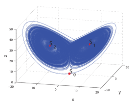
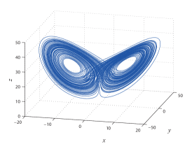
Figure 1: Numerical visualization of self-excited chaotic attractor in the Lorenz system. Global B-attractor (left subfigure), $d_{\rm L}(K)=\sup_{u\in K}d_{\rm L}(u)=d_{\rm L}(S_{0})=2.4013$ according to (92); global attractor (right subfigure), $d_{\rm L}(K)\approx 2.0565$ by numerical computation. Parameters: $r=28$, $\sigma=10$, $b=8/3$.

Here it is possible to check numerically that for the considered parameters the local attractor is a global attractor (i.e. there are no other attractors in the phase space). In this case the global B-attractor involves the chaotic local attractor, three unstable equilibria and their unstable manifolds attracted to the chaotic local attractor.

However it is known that for other values of parameters, e.g. $\sigma=10,\beta=8/3,\rho=24.5$ [103], the chaotic local attractor in the Lorenz system may be self-excited with respect to the zero unstable equilibrium only. In this case there are three coexisting minimal local attractors (see Fig. 2): chaotic local attractor and two trivial local attractors — stable equilibria $S_{1,2}$.

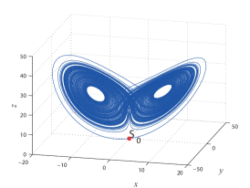
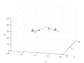
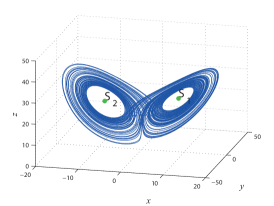
Figure 2: Numerical visualization of self-excited chaotic local attractor in the Lorenz system. Local B-attractor involves self-excited chaotic local attractor, unstable zero equilibrium and its unstable manifold attracted to the chaotic local attractor (left subfigure), $d_{\rm L}(K)=\sup_{u\in K}d_{\rm L}(u)=d_{\rm L}(S_{0})=2.3727$ according to (92). Trajectories with the initial data $(\pm 1.3276,\mp 9.7014,28.7491)$ tend to trivial local attractors — equilibria $S_{2,1}$ (middle subfigure), $d_{\rm L}(S_{2,1})=1.9989$. Global attractor is the union of three coexisting local attractors: self-excited chaotic local attractor and two trivial local attractors (right subfigure), $d_{\rm L}(K)\approx 2.0489$ by numerical computation. Parameters: $r=24.5$, $\sigma=10$, $b=8/3$.

Self-excited attractors in a multistable system can be found using the standard computational procedure, whereas there is no standard way of predicting the existence of hidden attractors in a system.

While the multistability is a property of system, the self-excited and hidden properties are the properties of attractor and its basin. For example, hidden attractors are attractors in systems with no equilibria or with only one stable equilibrium (a special case of multistability and coexistence of attractors).

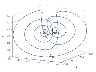
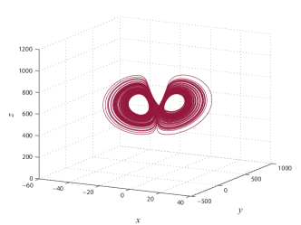
Figure 3: Numerical visualization of local B-attractor and hidden local attractor in the Glukhovsky-Dolghansky system. Local B-attractor involves outgoing separatrix (blue) of the saddle $S_{0}$ (red) attracted to the stable equilibria $S_{1,2}$ (green) (left subfigure). Hidden local attractor (magenta, $d_{\rm L}(K)\approx 2.1322$ by numerical computation) coexists with local B-attractor ($d_{\rm L}(K)=\sup_{u\in K}d_{\rm L}(u)=d_{\rm L}(S_{0})=2.8917$ by (98)). Global B-attractor involves the local B-attractor and the hidden local attractor.

In general, there is no straightforward way of predicting the existence or coexistence of hidden attractors in a system (see, e.g. [57, 79, 80, 77, 53, 67, 66, 54, 23, 51]). A numerical search of hidden attractors by evolutionary algorithms is discussed in [112, 113]. Recent examples of hidden attractors can be found in The European Physical Journal Special Topics: Multistability: Uncovering Hidden Attractors, 2015 (see [98, 11, 44, 114, 94, 97, 33, 81, 32, 104, 91, 108, 99]).

For example, in the Glukhovsky-Dolghansky system and the corresponding generalized Lorenz system (96) with parameters $r=700,a=0.0052,\sigma=ra,b=1$ a hidden chaotic local attractor can be found [66, 67] (see Fig. 3).

Remark that if a system is proved to be dissipative (i.e. it is possible to determine an absorbing bounded domain in the phase space such that all trajectories enter this domain within a finite time), then all self-excited or hidden local attractors of the system are inside this absorbing bounded domain and can be found numerically. However, in general, the determination of the number and mutual disposition of chaotic minimal local attractors in the phase space for a system may be a challenging problem [78] (see, e.g. the corresponding well-known problem for two-dimensional polynomial systems — the second part of 16th Hilbert problem on the number and mutual disposition of limit cycles [38]). Thus the advantage of the analytical method for the Lyapunov dimension estimation, suggested in Theorem 4, is that it is useful not only for the dissipative systems (see, e.g. estimation of the Lyapunov dimension for one of the Rossler systems [74]) but also allows one to estimate the Lyapunov dimension of invariant set without localization of the set in the phase space.

Remark that, from a computational perspective, it is not feasible to numerically check Property 1 for all initial states of the phase space of a dynamical system. A natural generalization of the notion of an attractor is the consideration of the weaker attraction requirements: almost everywhere or on a set of positive measure (see, e.g., [85]). See also trajectory attractors [96, 13, 17]. In numerical computations, to distinguish an artificial computer generated chaos from a real behavior of the system, one can consider the shadowing property of the system (see, e.g., the survey in [92]).

We can typically see an attractor (or global attractor) in numerical experiments. The notion of a B-attractor is mostly used in the theory of dimensions, where we consider invariant sets covered by balls. The uniform attraction requirement in Property 3 implies that a global B-attractor involves a set of stationary points $\mathcal{S}$ and the corresponding unstable manifolds $W^{u}(\mathcal{S})=\left\{{u}_{0}\in\mathbb{R}^{n}~{}|~{}\lim_{t\to-\infty}\rho(\mathcal{S},\varphi^{t}(u_{0}))=0\right\}$ (see, e.g., [18, 15]). The same is true for B-attractor if the considered neighborhood $K_{\varepsilon}$ in Property 3 contains some of the stationary points from $\mathcal{S}$. This allows one to get analytical estimations of the Lyapunov dimension for B-attractors and even formulas since the local Lyapunov dimension at a stationary point can be easily obtained analytically (but this does not help for chaotic minimal local attractors, hidden B-attractors since they do not involve any stationary points).

From a computational perspective, numerical check of Property 3 is also difficult. Therefore, if the basin of attraction involves unstable manifolds of equilibria, then computing the minimal attractor and the unstable manifolds that are attracted to it may be regarded as an approximation of minimal B-attractor. For example, consider the visualization of the classical Lorenz attractor from the neighborhood of the zero saddle equilibria. Note that a minimal global attractor involves the set $\mathcal{S}$ and its basin of attraction involves the set $W^{u}(\mathcal{S})$.

For the computation of the Lyapunov dimension of an attractor $A$ we consider a sufficiently large time $T$ and a sufficiently dense grid of points $A_{\rm grid}$ on the attractor, compute the local Lyapunov dimensions by the corresponding Kaplan-Yorke formula $d_{\rm L}^{\rm KY}(\{\operatorname{\nu}_{i}(T,u)\}_{1}^{n})$, and take maximum on the grid: $\max_{u\in A_{\rm grid}}d_{\rm L}^{\rm KY}(\{\operatorname{\nu}_{i}(T,u)\}_{1}^{n})$.

Since numerically we can check only that all points of the grid belong to the basin of attraction, the following remak is useful. Let a point $u_{0}$ belongs to the basin of attraction of attractor $A$. Consider the union of the semi-orbit $\gamma^{+}(u_{0})=\{\varphi^{t}(u_{0}),t\geq 0\}$ and attractor $A$: $K(u_{0})=A\cup\gamma^{+}(u_{0})$. According to the definition of the basin of attraction, $\omega$-limit set of $\varphi^{t}(u_{0})$ belong to $A$, thus the set $K(u_{0})$ is compact and invariant. Since $A\supseteq K(\varphi^{t}(u_{0}))\supseteq K(u_{0})$, we have

$$d_{\rm L}(\varphi^{t},A)=\max_{u\in A}d_{\rm L}(\varphi^{t},u)\leq\max_{u\in K(\varphi^{t}(u_{0}))}d_{\rm L}(\varphi^{t},u)\leq\max_{u\in K(u_{0})}d_{\rm L}(\varphi^{t},u).$$

Since $\rho\big{(}K(u_{0}),K(\varphi^{t}(u_{0}))\big{)}\to 0$ for $t\to+\infty$, from the properties of decreasing (34) and continuity (Lemma 3), it follows that

$$d_{\rm L}=\liminf_{t\to+\infty}\max_{u\in K(\varphi^{t}(u_{0}))}d_{\rm L}(\varphi^{t},u).$$

8 Computation of the finite-time Lyapunov exponents and dimension in MATLAB

The singular value decomposition (SVD) of a fundamental matrix $D\varphi^{t}(u_{0})$ has the from

$$D\varphi^{t}(u_{0})={\rm U}(t,u_{0}){\rm\Sigma}(t,u_{0}){\rm V}^{T}(t,u_{0}):\quad{\rm U}(t,u_{0})^{T}{\rm U}(t,u_{0})\equiv I\equiv{\rm V}(t,u_{0})^{T}{\rm V}(t,u_{0}),$$

where ${\rm\Sigma}(t)=\text{\rm diag}\{\sigma_{1}(t,u_{0}),...,\sigma_{n}(t,u_{0})\}$ is a diagonal matrix with positive real diagonal entries — singular values. We now give a MATLAB implementation [67] of the discrete SVD method for computing finite-time Lyapunov exponents $\{\operatorname{\nu}_{i}(t,u_{0})\}_{1}^{n}$ based on the product SVD algorithm (see, e.g., [105, 25]). For the computation of the Lyapunov dimension of an attractor by the considered code one has to consider a sufficiently large time $T$ and a grid of points on the attractor $K_{\rm grid}$, compute the local Lyapunov dimensions by the corresponding Kaplan-Yorke formula $d_{\rm L}^{\rm KY}(\{\operatorname{\nu}_{i}(T,u)\}_{1}^{n})$ (see, e.g. [58]), and takes maximum on the grid: $\max_{u\in K_{\rm grid}}d_{\rm L}^{\rm KY}(\{\operatorname{\nu}_{i}(T,u)\}_{1}^{n}).$

Listing 1: productSVD.m – product SVD algorithm

⬇

1function [U, R, V] = productSVD(initFactorization, nIterations)

2% Parameters:

3% initFactorization - the array contains factor matrices of the

4% fundamental matrix X, such that:

5% X = initFactorization(:,:,1) * ... * initFactorization(:,:,end);

6% nIterations - the number of iterations in the product SVD algorithm.

7

8% dimOde - dimension of the ODEs, nFactors - the number of factor matrices

9[~, dimOde, nFactors] = size(initFactorization);

10

11% A - 2d array of matrices storing the factor matrices at each iteration

12A = zeros(dimOde, dimOde, nFactors, nIterations);

13A(:, :, :, 1) = initFactorization;

14

15% Q - array of matrices storing orhogonal matrices of the QR decomposition

16Q = zeros(dimOde, dimOde, nFactors+1);

17

18% U, V - orthogonal matrices in the SVD decomposition

19U = eye(dimOde); V = eye(dimOde);

20

21% R - array of upper triangular factor matrices, such that after

22% the last iteration \Sigma = R(:,:,1) * ... * R(:,:,end)

23R = zeros(dimOde, dimOde, nFactors);

24

25% Main loop

26for iIteration = 1 : nIterations

27 Q(:, :, nFactors + 1) = eye(dimOde, dimOde);

28 for jFactor = nFactors : -1 : 1

29 C = A(:, :, jFactor, iIteration) * Q(:, :, jFactor+1);

30 [Q(:, :, jFactor), R(:, :, jFactor)] = qr(C);

31 for kCoord = 1 : dimOde

32 if R(kCoord, kCoord, jFactor) < 0

33 R(kCoord, :, jFactor) = -1 * R(kCoord, :, jFactor);

34 Q(:, kCoord, jFactor) = -1 * Q(:, kCoord, jFactor);

35 end;

36 end;

37 end;

38

39 if mod(iIteration, 2) == 1

40 U = U * Q(:, :, 1);

41 else

42 V = V * Q(:, :, 1);

43 end

44

45 for jFactor = 1 : nFactors

46 A(:, :, jFactor, iIteration + 1) = R(:, :, nFactors-jFactor+1)’;

47 end

48end

49

50end

Listing 2: computeLEs.m – computation of the Lyapunov exponents

⬇

1function LEs = computeLEs(extOde, initPoint, tStep, ...

2 nFactors, nSvdIterations, odeSolverOptions)

3% Parameters:

4% extOde - extended ODE system (system of ODEs + var. eq.);

5% initPoint - initial point;

6% tStep - time-step in the factorization procedure;

7% nFactors - number of factor matrices in the factorization procedure;

8% nSvdIterations - number of iterations in the product SVD algoritm;

9% odeSolverOptions - solver options (sover = ode45);

10

11% Dimension of the ODE :

12dimOde = length(initPoint);

13

14% Dimension of the extended ODE (ODE + Var. Eq.):

15dimExtOde = dimOde * (dimOde + 1);

16

17tBegin = 0; tEnd = tStep;

18tSpan = [tBegin, tEnd];

19initFundMatrix = eye(dimOde);

20initCond = [initPoint(:); initFundMatrix(:)];

21

22X = zeros(dimOde, dimOde, nFactors);

23

24% Main loop : factorization of the fundamental matrix

25for iFactor = 1 : nFactors

26 [~, extOdeSolution] = ode45(extOde, tSpan, initCond, odeSolverOptions);

27

28 X(:, :, iFactor) = reshape(...

29 extOdeSolution(end, (dimOde + 1) : dimExtOde), ...

30 dimOde, dimOde);

31 currInitPoint = extOdeSolution(end, 1 : dimOde);

32 currInitFundMatrix = eye(dimOde);

33

34 tBegin = tBegin + tStep;

35 tEnd = tEnd + tStep;

36 tSpan = [tBegin, tEnd];

37 initCond = [currInitPoint(:); currInitFundMatrix(:)];

38end

39

40% Product SVD of factorization X of the fundamental matrix

41[~, R, ~] = productSVD(X, nSvdIterations);

42

43% Computation of the Lyapunov exponents

44LEs = zeros(1, dimOde);

45for jFactor = 1 : nFactors

46 LEs = LEs + log(diag(R(:, :, jFactor))’);

47end;

48finalTime = tStep * nFactors;

49LEs = LEs / finalTime;

50

51end

Listing 3: lyapunovDim.m – computation of the Lyapunov dimension

⬇

1function LD = lyapunovDim( LEs )

2% For the given array of finite-time Lyapunov exponents at a point the function

3% computes the local Lyapunov dimension by the Kaplan-Yorke formula.

4

5% Parameters:

6% LEs - array of the finite-time Lyapunov exponents.

7

8% Initialization of the local Lyapunov dimension:

9LD = 0;

10

11% Number of LEs :

12nLEs = length(LEs);

13

14% Sorted LEs :

15sortedLEs = sort(LEs, ’descend’);

16

17% Main loop :

18leSum = sortedLEs(1);

19if ( sortedLEs(1) > 0 )

20 for i = 1 : nLEs-1

21 if sortedLEs(i+1) ~= 0

22 LD = i + leSum / abs( sortedLEs(i+1) );

23 leSum = leSum + sortedLEs(i+1);

24 if leSum < 0

25 break;

26 end

27 end

28 end

29end

30end

Listing 4: genLorenzSyst.m – generalized Lorenz system (96) along with the variational equation

⬇

1function OUT = genLorenzSyst(t, x, r, sigma, b, a)

2

3% Generalized Lorenz system with

4% parameters: r sigma b a

5

6OUT(1) = sigma*(x(2) - x(1)) - a*x(2)*x(3);

7OUT(2) = r*x(1) - x(2) - x(1)*x(3);

8OUT(3) = -b*x(3) + x(1)*x(2);

9

10% Jacobian at the point [x(1), x(2), x(3)]

11J = [-sigma, sigma-a*x(3), -a*x(2);

12 r-x(3), -1, -x(1);

13 x(2), x(1), -b];

14

15X = [x(4), x(7), x(10);

16 x(5), x(8), x(11);

17 x(6), x(9), x(12)];

18

19% Variational equation

20OUT(4:12) = J*X;

Listing 5: main.m – computation of the Lyapunov exponents and local Lyapunov dimension for the hidden attractor of generalized Lorenz system (96)

⬇

1function main

2

3% Parameters of generalized Lorenz system

4% that correspond to the hidden attractor

5r = 700; sigma = 4; b = 1; a = 0.0052;

6

7% Initial point for the trajectory which visualizes the hidden attractor

8x0 = [-14.551336132013954 -173.86811769236883 718.92035664071227];

9

10tStep = 0.1;

11nFactors = 10000;

12nSvdIterations = 3;

13

14% ODE solver parameters

15acc = 1e-8; RelTol = acc; AbsTol = acc; InitialStep = acc/10;

16odeSolverOptions = odeset(’RelTol’, RelTol, ’AbsTol’, AbsTol, ...

17 ’InitialStep’, InitialStep, ’NormControl’, ’on’);

18

19LEs = computeLEs(@(t, x) genLorenzSyst(t, x, r, sigma, b, a), ...

20 x0, tStep, nFactors, nSvdIterations, odeSolverOptions);

21

22fprintf(’Lyapunov exponents: %6.4f, %6.4f, %6.4f\n’, LEs);

23

24LD = lyapunovDim(LEs);

25

26fprintf(’Lyapunov dimension: %6.4f\n’, LD);

27

28end

Conclusions

In this survey for finite dimensional dynamical systems in Euclidean space we have tried to discuss rigorously the connection between the works by Kaplan and Yorke (the concept of Lyapunov dimension, 1979), Douady and Oesterlé (estimation of Hausdorff dimension via the Lyapunov dimension of maps, 1980), Constantin, Eden, Foias, and Temam (estimation of Hausdorff dimension via the Lyapunov exponents and dimension of dynamical systems, 1985-90), Leonov (estimation of the Lyapunov dimension via the direct Lyapunov method, 1991), and numerical methods for the computation of Lyapunov exponents and Lyapunov dimension. Remark that in the numerical estimations we can consider only finite time and get finite-time Lyapunov exponents, thus we have discussed the justification of Kaplan-Yorke formula with respect to finite-time Lyapunov exponent, by the Douady–Oesterlé theorem for maps. For various self-excited and hidden attractors of well-known dynamical systems, the numerical values, analytical estimations and formulas of the Lyapunov dimension are given.

References

- Abarbanel et al., [1991] Abarbanel, H., Brown, R., and Kennel, M. (1991). Variation of Lyapunov exponents on a strange attractor. Journal of Nonlinear Science, 1(2):175–199.
- Adrianova, [1998] Adrianova, L. Y. (1998). Introduction to Linear systems of Differential Equations. American Mathematical Society, Providence, Rhode Island.
- Aleksandrov and Pasynkov, [1973] Aleksandrov, P. and Pasynkov, B. (1973). Introduction to Dimension Theory (in Russian). Nauka, Moscow.
- Babin and Vishik, [1992] Babin, A. V. and Vishik, M. I. (1992). Attractors of Evolution Equations. North-Holland, Amsterdam.
- Barabanov, [2005] Barabanov, E. (2005). Singular exponents and properness criteria for linear differential systems. Differential Equations, 41:151–162.
- Barreira and Gelfert, [2011] Barreira, L. and Gelfert, K. (2011). Dimension estimates in smooth dynamics: a survey of recent results. Ergodic Theory and Dynamical Systems, 31:641–671.
- Barreira and Schmeling, [2000] Barreira, L. and Schmeling, J. (2000). Sets of “Non-typical” points have full topological entropy and full Hausdorff dimension. Israel Journal of Mathematics, 116(1):29–70.
- Bogoliubov and Krylov, [1937] Bogoliubov, N. and Krylov, N. (1937). La theorie generalie de la mesure dans son application a l’etude de systemes dynamiques de la mecanique non-lineaire. Ann. Math. II (in French) (Annals of Mathematics), 38(1):65–113.
- Boichenko and Leonov, [1998] Boichenko, V. and Leonov, G. (1998). Lyapunov’s direct method in estimates of topological entropy. Journal of Mathematical Sciences, 91(6):3370–3379.
- Boichenko et al., [2005] Boichenko, V. A., Leonov, G. A., and Reitmann, V. (2005). Dimension Theory for Ordinary Differential Equations. Teubner, Stuttgart.
- Brezetskyi et al., [2015] Brezetskyi, S., Dudkowski, D., and Kapitaniak, T. (2015). Rare and hidden attractors in van der Pol-Duffing oscillators. European Physical Journal: Special Topics, 224(8):1459–1467.
- Bylov et al., [1966] Bylov, B. E., Vinograd, R. E., Grobman, D. M., and Nemytskii, V. V. (1966). Theory of characteristic exponents and its applications to problems of stability (in Russian). Nauka, Moscow.
- Chepyzhov and Vishik, [2002] Chepyzhov, V. and Vishik, M. (2002). Attractors for equations of mathematical physics. American Mathematical Society, Providence, Rhode Island.
- Choquet and Foias, [1975] Choquet, G. and Foias, C. (1975). Solution d’un probleme sur les iteres d’un operateur positif sur et proprietes de moyennes associees. Annales de l’institut Fourier (in French), 25(3-4):109–129.
- Chueshov, [2002] Chueshov, I. (2002). Introduction to the Theory of Infinite-dimensional Dissipative Systems. Electronic library of mathematics. ACTA.
- Chueshov, [2015] Chueshov, I. (2015). Dynamics of Quasi-Stable Dissipative Systems. Springer.
- Chueshov and Siegmund, [2005] Chueshov, I. and Siegmund, S. (2005). On dimension and metric properties of trajectory attractors. Journal of Dynamics and Differential Equations, 17(4):621–641.
- Chueshov, [1993] Chueshov, I. D. (1993). Global attractors in the nonlinear problems of mathematical physics. Russian Mathematical Surveys, 48(3):135–162.
- Constantin and Foias, [1985] Constantin, P. and Foias, C. (1985). Global Lyapunov exponents, Kaplan-Yorke formulas and the dimension of the attractors for 2D Navier-Stokes equations. Communications on Pure and Applied Mathematics, 38(1):1–27.
- Constantin et al., [1985] Constantin, P., Foias, C., and Temam, R. (1985). Attractors representing turbulent flows. Memoirs of the American Mathematical Society, 53(314).
- Cvitanović et al., [2012] Cvitanović, P., Artuso, R., Mainieri, R., Tanner, G., and Vattay, G. (2012). Chaos: Classical and Quantum. Niels Bohr Institute, Copenhagen. http://ChaosBook.org.
- Czornik et al., [2013] Czornik, A., Nawrat, A., and Niezabitowski, M. (2013). Lyapunov exponents for discrete time-varying systems. Studies in Computational Intelligence, 440:29–44.
- Danca et al., [2016] Danca, M.-F., Feckan, M., Kuznetsov, N., and Chen, G. (2016). Looking more closely at the Rabinovich-Fabrikant system. International Journal of Bifurcation and Chaos, 26(02). art. num. 1650038.
- Dellnitz and Junge, [2002] Dellnitz, M. and Junge, O. (2002). Set oriented numerical methods for dynamical systems. In Handbook of Dynamical Systems, volume 2, pages 221–264. Elsevier Science.
- Dieci and Elia, [2008] Dieci, L. and Elia, C. (2008). SVD algorithms to approximate spectra of dynamical systems. Mathematics and Computers in Simulation, 79(4):1235–1254.
- Doering et al., [1987] Doering, C., Gibbon, J., Holm, D., and Nicolaenko, B. (1987). Exact Lyapunov dimension of the universal attractor for the complex Ginzburg-Landau equation. Phys. Rev. Lett., 59:2911–2914.
- Douady and Oesterle, [1980] Douady, A. and Oesterle, J. (1980). Dimension de Hausdorff des attracteurs. C.R. Acad. Sci. Paris, Ser. A. (in French), 290(24):1135–1138.
- [28] Eden, A. (1989a). An abstract theory of L-exponents with applications to dimension analysis (PhD thesis). Indiana University.
- [29] Eden, A. (1989b). Local Lyapunov exponents and a local estimate of Hausdorff dimension. ESAIM: Mathematical Modelling and Numerical Analysis - Modelisation Mathematique et Analyse Numerique, 23(3):405–413.
- Eden, [1990] Eden, A. (1990). Local estimates for the Hausdorff dimension of an attractor. Journal of Mathematical Analysis and Applications, 150(1):100–119.
- Eden et al., [1991] Eden, A., Foias, C., and Temam, R. (1991). Local and global Lyapunov exponents. Journal of Dynamics and Differential Equations, 3(1):133–177. [Preprint No. 8804, The Institute for Applied Mathematics and Scientific Computing, Indiana University, 1988].
- Feng et al., [2015] Feng, Y., Pu, J., and Wei, Z. (2015). Switched generalized function projective synchronization of two hyperchaotic systems with hidden attractors. European Physical Journal: Special Topics, 224(8):1593–1604.
- Feng and Wei, [2015] Feng, Y. and Wei, Z. (2015). Delayed feedback control and bifurcation analysis of the generalized Sprott B system with hidden attractors. European Physical Journal: Special Topics, 224(8):1619–1636.
- Frederickson et al., [1983] Frederickson, P., Kaplan, J., Yorke, E., and Yorke, J. (1983). The Liapunov dimension of strange attractors. Journal of Differential Equations, 49(2):185–207.
- Gelfert, [2003] Gelfert, K. (2003). Maximum local Lyapunov dimension bounds the box dimension. Direct proof for invariant sets on Riemannian manifolds. Z. Anal. Anwend., 22:553–568.
- Glukhovskii and Dolzhanskii, [1980] Glukhovskii, A. B. and Dolzhanskii, F. V. (1980). Three-component geostrophic model of convection in a rotating fluid. Academy of Sciences, USSR, Izvestiya, Atmospheric and Oceanic Physics (in Russian), 16:311–318.
- Gundlach and Steinkamp, [2000] Gundlach, V. and Steinkamp, O. (2000). Products of random rectangular matrices. Mathematische Nachrichten, 212(1):51–76.
- Hilbert, [1902] Hilbert, D. (1901-1902). Mathematical problems. Bull. Amer. Math. Soc., (8):437–479.
- Horn and Johnson, [1994] Horn, R. and Johnson, C. (1994). Topics in Matrix Analysis. Cambridge University Press, Cambridge.
- Hunt, [1996] Hunt, B. (1996). Maximum local Lyapunov dimension bounds the box dimension of chaotic attractors. Nonlinearity, 9(4):845–852.
- Hurewicz and Wallman, [1941] Hurewicz, W. and Wallman, H. (1941). Dimension Theory. Princeton University Press, Princeton.
- Ilyashenko and Li, [1999] Ilyashenko, Y. and Li, W. (1999). Nonlocal Bifurcations. American Mathematical Society, Rhode Island.
- Izobov, [2012] Izobov, N. A. (2012). Lyapunov exponents and stability. Cambridge Scientific Publischers, Cambridge.
- Jafari et al., [2015] Jafari, S., Sprott, J., and Nazarimehr, F. (2015). Recent new examples of hidden attractors. European Physical Journal: Special Topics, 224(8):1469–1476.
- Kaplan and Yorke, [1979] Kaplan, J. L. and Yorke, J. A. (1979). Chaotic behavior of multidimensional difference equations. In Functional Differential Equations and Approximations of Fixed Points, pages 204–227. Springer, Berlin.
- Kolmogorov, [1959] Kolmogorov, A. (1959). On entropy per unit time as a metric invariant of automorphisms. Dokl. Akad. Nauk SSSR (In Russian), 124(4):754–755.
- Kuczma and Gilányi, [2009] Kuczma, M. and Gilányi, A. (2009). An Introduction to the Theory of Functional Equations and Inequalities: Cauchy’s Equation and Jensen’s Inequality. Birkhäuser Basel.
- Kunze and Kupper, [2001] Kunze, M. and Kupper, T. (2001). Non-smooth dynamical systems: An overview. In Ergodic Theory, Analysis, and Efficient Simulation of Dynamical Systems, pages 431–452. Springer.
- Kuratowski, [1966] Kuratowski, K. (1966). Topology. Academic press, New York.
- [50] Kuznetsov, N. (2016a). Estimation of Lyapunov dimension via the Leonov method. arXiv. http://arxiv.org/pdf/1602.05410v1.pdf.
- [51] Kuznetsov, N. (2016b). Hidden attractors in fundamental problems and engineering models. A short survey. Lecture Notes in Electrical Engineering, 371:13–25. (plenary lecture at AETA 2015: Recent Advances in Electrical Engineering and Related Sciences).
- Kuznetsov et al., [2016] Kuznetsov, N., Alexeeva, T., and Leonov, G. (2016). Invariance of Lyapunov exponents and Lyapunov dimension for regular and irregular linearizations. Nonlinear Dynamics. (arXiv e-prints 1410.2016v2, 2014).
- Kuznetsov and Leonov, [2014] Kuznetsov, N. and Leonov, G. (2014). Hidden attractors in dynamical systems: systems with no equilibria, multistability and coexisting attractors. IFAC Proceedings Volumes (IFAC-PapersOnline), 19:5445–5454.
- Kuznetsov et al., [2015] Kuznetsov, N., Leonov, G. A., and Mokaev, T. N. (2015). Hidden attractor in the Rabinovich system. arXiv:1504.04723v1. http://arxiv.org/pdf/1504.04723v1.pdf.
- [55] Kuznetsov, N. V., Alexeeva, T., and Leonov, G. A. (2014a). Invariance of Lyapunov characteristic exponents, Lyapunov exponents, and Lyapunov dimension for regular and non-regular linearizations. arXiv:1410.2016v2. (accepted to Nonlinear Dynamics).
- Kuznetsov and Leonov, [2005] Kuznetsov, N. V. and Leonov, G. A. (2005). On stability by the first approximation for discrete systems. In 2005 International Conference on Physics and Control, PhysCon 2005, volume Proceedings Volume 2005, pages 596–599. IEEE.
- Kuznetsov et al., [2010] Kuznetsov, N. V., Leonov, G. A., and Vagaitsev, V. I. (2010). Analytical-numerical method for attractor localization of generalized Chua’s system. IFAC Proceedings Volumes (IFAC-PapersOnline), 4(1):29–33.
- [58] Kuznetsov, N. V., Mokaev, T. N., and Vasilyev, P. A. (2014b). Numerical justification of Leonov conjecture on Lyapunov dimension of Rossler attractor. Commun Nonlinear Sci Numer Simulat, 19:1027–1034.
- Ladyzhenskaya, [1987] Ladyzhenskaya, O. (1987). Determination of minimal global attractors for the Navier-Stokes equations and other partial differential equations. Russian Mathematical Surveys, 42(6):25–60.
- Ladyzhenskaya, [1991] Ladyzhenskaya, O. A. (1991). Attractors for semi-groups and evolution equations. Cambridge University Press.
- Ledrappier, [1981] Ledrappier, F. (1981). Some relations between dimension and Lyapounov exponents. Communications in Mathematical Physics, 81(2):229–238.
- Leonov, [2002] Leonov, G. (2002). Lyapunov dimension formulas for Henon and Lorenz attractors. St.Petersburg Mathematical Journal, 13(3):453–464.
- [63] Leonov, G., Alexeeva, T., and Kuznetsov, N. (2015a). Analytic exact upper bound for the Lyapunov dimension of the Shimizu-Morioka system. Entropy, 17(7):5101.
- [64] Leonov, G., Kuznetsov, N., Korzhemanova, N., and Kusakin, D. (2015b). The Lyapunov dimension formula for the global attractor of the Lorenz system. arXiv, http://arxiv.org/pdf/1508.07498v1.pdf.
- [65] Leonov, G., Kuznetsov, N., Korzhemanova, N., and Kusakin, D. (2015c). Lyapunov dimension formula of attractors in the Tigan and Yang systems. arXiv:1510.01492v1, http://arxiv.org/pdf/1510.01492v1.pdf.
- [66] Leonov, G., Kuznetsov, N., and Mokaev, T. (2015d). Hidden attractor and homoclinic orbit in Lorenz-like system describing convective fluid motion in rotating cavity. Communications in Nonlinear Science and Numerical Simulation, 28:166–174.
- [67] Leonov, G., Kuznetsov, N., and Mokaev, T. (2015e). Homoclinic orbits, and self-excited and hidden attractors in a Lorenz-like system describing convective fluid motion. Eur. Phys. J. Special Topics, 224(8):1421–1458.
- Leonov and Lyashko, [1993] Leonov, G. and Lyashko, S. (1993). Eden’s hypothesis for a Lorentz system. Vestnik St. Petersburg University: Mathematics, 26(3):15–18. [Transl. from Russian. Vestnik Sankt-Peterburgskogo Universiteta. Ser 1. Matematika, 26(3), 14-16].
- [69] Leonov, G., Pogromsky, A., and Starkov, K. (2012a). Erratum to ”The dimension formula for the Lorenz attractor” [Phys. Lett. A 375 (8) (2011) 1179]. Physics Letters A, 376(45):3472 – 3474.
- Leonov and Poltinnikova, [2005] Leonov, G. and Poltinnikova, M. (2005). On the Lyapunov dimension of the attractor of Chirikov dissipative mapping. AMS Translations. Proceedings of St.Petersburg Mathematical Society. Vol. X, 224:15–28.
- Leonov, [1991] Leonov, G. A. (1991). On estimations of Hausdorff dimension of attractors. Vestnik St. Petersburg University: Mathematics, 24(3):38–41. [Transl from Russian. Vestnik Leningradskogo Universiteta. Mathematika, 24(3), 1991, pp. 41-44].
- Leonov, [2008] Leonov, G. A. (2008). Strange attractors and classical stability theory. St.Petersburg University Press, St.Petersburg.
- Leonov, [2012] Leonov, G. A. (2012). Lyapunov functions in the attractors dimension theory. Journal of Applied Mathematics and Mechanics, 76(2):129–141.
- Leonov and Boichenko, [1992] Leonov, G. A. and Boichenko, V. A. (1992). Lyapunov’s direct method in the estimation of the Hausdorff dimension of attractors. Acta Applicandae Mathematicae, 26(1):1–60.
- [75] Leonov, G. A., Kuznetsov, N., and Mokaev, T. N. (2015f). The Lyapunov dimension formula of self-excited and hidden attractors in the Glukhovsky-Dolzhansky system. arXiv:1509.09161. http://arxiv.org/pdf/1509.09161v1.pdf.
- Leonov and Kuznetsov, [2007] Leonov, G. A. and Kuznetsov, N. V. (2007). Time-varying linearization and the Perron effects. International Journal of Bifurcation and Chaos, 17(4):1079–1107.
- Leonov and Kuznetsov, [2013] Leonov, G. A. and Kuznetsov, N. V. (2013). Hidden attractors in dynamical systems. From hidden oscillations in Hilbert-Kolmogorov, Aizerman, and Kalman problems to hidden chaotic attractors in Chua circuits. International Journal of Bifurcation and Chaos, 23(1). art. no. 1330002.
- Leonov and Kuznetsov, [2015] Leonov, G. A. and Kuznetsov, N. V. (2015). On differences and similarities in the analysis of Lorenz, Chen, and Lu systems. Applied Mathematics and Computation, 256:334–343.
- Leonov et al., [2011] Leonov, G. A., Kuznetsov, N. V., and Vagaitsev, V. I. (2011). Localization of hidden Chua’s attractors. Physics Letters A, 375(23):2230–2233.
- [80] Leonov, G. A., Kuznetsov, N. V., and Vagaitsev, V. I. (2012b). Hidden attractor in smooth Chua systems. Physica D: Nonlinear Phenomena, 241(18):1482–1486.
- Li et al., [2015] Li, C., Hu, W., Sprott, J., and Wang, X. (2015). Multistability in symmetric chaotic systems. European Physical Journal: Special Topics, 224(8):1493–1506.
- Lorenz, [1963] Lorenz, E. N. (1963). Deterministic nonperiodic flow. J. Atmos. Sci., 20(2):130–141.
- Lyapunov, [1892] Lyapunov, A. M. (1892). The General Problem of the Stability of Motion (in Russian). Kharkov. [English transl. Academic Press, NY, 1966].
- Millionschikov, [1976] Millionschikov, V. M. (1976). A formula for the entropy of smooth dynamical systems. Differencial’nye Uravenija (in Russian), 12(12):2188–2192, 2300.
- Milnor, [2006] Milnor, J. (2006). Attractor. Scholarpedia, 1(11). doi:10.4249/scholarpedia.1815.
- Noack and Reitmann, [1996] Noack, A. and Reitmann, V. (1996). Hausdorff dimension estimates for invariant sets of time-dependent vector fields. Z. Anal. Anwend., 15:457–473.
- Oseledec, [1968] Oseledec, V. (1968). Multiplicative ergodic theorem: Characteristic Lyapunov exponents of dynamical systems. In Transactions of the Moscow Mathematical Society, volume 19, pages 179–210.
- Ott et al., [1984] Ott, E., Withers, W., and Yorke, J. (1984). Is the dimension of chaotic attractors invariant under coordinate changes? Journal of Statistical Physics, 36(5-6):687–697.
- Ott and Yorke, [2008] Ott, W. and Yorke, J. (2008). When Lyapunov exponents fail to exist. Phys. Rev. E, 78:056203.
- Pesin, [1977] Pesin, Y. (1977). Characteristic Lyapunov exponents and smooth ergodic theory. Russian Mathematical Surveys, 32(4):55–114.
- Pham et al., [2015] Pham, V., Vaidyanathan, S., Volos, C., and Jafari, S. (2015). Hidden attractors in a chaotic system with an exponential nonlinear term. European Physical Journal: Special Topics, 224(8):1507–1517.
- Pilyugin, [2011] Pilyugin, S. (2011). Theory of pseudo-orbit shadowing in dynamical systems. Differential Equations, 47(13):1929–1938.
- Pogromsky and Matveev, [2011] Pogromsky, A. Y. and Matveev, A. S. (2011). Estimation of topological entropy via the direct Lyapunov method. Nonlinearity, 24(7):1937.
- Saha et al., [2015] Saha, P., Saha, D., Ray, A., and Chowdhury, A. (2015). Memristive non-linear system and hidden attractor. European Physical Journal: Special Topics, 224(8):1563–1574.
- Schmeling, [1998] Schmeling, J. (1998). A dimension formula for endomorphisms – the Belykh family. Ergodic Theory and Dynamical Systems, 18:1283–1309.
- Sell, [1996] Sell, G. R. (1996). Global attractors for the three-dimensional Navier-Stokes equations. Journal of Dynamics and Differential Equations, 8(1):1–33.
- Semenov et al., [2015] Semenov, V., Korneev, I., Arinushkin, P., Strelkova, G., Vadivasova, T., and Anishchenko, V. (2015). Numerical and experimental studies of attractors in memristor-based Chua’s oscillator with a line of equilibria. Noise-induced effects. European Physical Journal: Special Topics, 224(8):1553–1561.
- Shahzad et al., [2015] Shahzad, M., Pham, V.-T., Ahmad, M., Jafari, S., and Hadaeghi, F. (2015). Synchronization and circuit design of a chaotic system with coexisting hidden attractors. European Physical Journal: Special Topics, 224(8):1637–1652.
- Sharma et al., [2015] Sharma, P., Shrimali, M., Prasad, A., Kuznetsov, N., and Leonov, G. (2015). Control of multistability in hidden attractors. Eur. Phys. J. Special Topics, 224(8):1485–1491.
- Shimizu and Morioka, [1980] Shimizu, T. and Morioka, N. (1980). On the bifurcation of a symmetric limit cycle to an asymmetric one in a simple model. Physics Letters A, 76(3-4):201 – 204.
- Sinai, [1959] Sinai, Y. (1959). On the notion of entropy of dynamical systems. Dokl. Akad. Nauk SSSR (In Russian), 124(4):768–771.
- Smith, [1986] Smith, R. (1986). Some application of Hausdorff dimension inequalities for ordinary differential equation. Proc. Royal Society Edinburg, 104A:235–259.
- Sparrow, [1982] Sparrow, C. (1982). The Lorenz Equations: Bifurcations, Chaos, and Strange Attractors. Applied Mathematical Sciences. Springer New York.
- Sprott, [2015] Sprott, J. (2015). Strange attractors with various equilibrium types. European Physical Journal: Special Topics, 224(8):1409–1419.
- Stewart, [1997] Stewart, D. E. (1997). A new algorithm for the SVD of a long product of matrices and the stability of products. Electronic Transactions on Numerical Analysis, 5:29–47.
- Temam, [1997] Temam, R. (1997). Infinite-dimensional Dynamical Systems in Mechanics and Physics. Springer-Verlag, New York, 2nd edition.
- Tigan and Opris, [2008] Tigan, G. and Opris, D. (2008). Analysis of a 3d chaotic system. Chaos, Solitons & Fractals, 36(5):1315–1319.
- Vaidyanathan et al., [2015] Vaidyanathan, S., Pham, V.-T., and Volos, C. (2015). A 5-D hyperchaotic Rikitake dynamo system with hidden attractors. European Physical Journal: Special Topics, 224(8):1575–1592.
- Yang and Chen, [2008] Yang, Q. and Chen, G. (2008). A chaotic system with one saddle and two stable node-foci. International Journal of Bifurcation and Chaos, 18:1393–1414.
- Young, [2013] Young, L.-S. (2013). Mathematical theory of Lyapunov exponents. Journal of Physics A: Mathematical and Theoretical, 46(25):254001.
- Zakrzhevsky et al., [2007] Zakrzhevsky, M., Schukin, I., and Yevstignejev, V. (2007). Scientific Proc. Riga Technical Univ. Transp. Engin., 6:79.
- Zelinka, [2015] Zelinka, I. (2015). A survey on evolutionary algorithms dynamics and its complexity – Mutual relations, past, present and future. Swarm and Evolutionary Computation, 25:2–14.
- Zelinka, [2016] Zelinka, I. (2016). Evolutionary identification of hidden chaotic attractors. Engineering Applications of Artificial Intelligence, 50:159–167. 10.1016/j.engappai.2015.12.002.
- Zhusubaliyev et al., [2015] Zhusubaliyev, Z., Mosekilde, E., Churilov, A., and Medvedev, A. (2015). Multistability and hidden attractors in an impulsive Goodwin oscillator with time delay. European Physical Journal: Special Topics, 224(8):1519–1539.