Matter-Sector Lorentz Violation in Binary Pulsars

Abstract

Violations of local Lorentz invariance in the gravitationally coupled matter sector have yet to be sought in strong-gravity systems. We present the implications of matter-sector Lorentz violation for orbital perturbations in pulsar systems and show that the analysis of pulsar data can provide sensitivities to these effects that exceed the current reach of solar system and laboratory tests by several orders of magnitude.

I Introduction

Since the discovery of pulsars hewish and the observation of binary-pulsar systems ht , pulsars have been used to test many aspects of our current best theory of the gravitational field, General Relativity (GR) stairs . When coupled to the Standard Model (SM) of particle physics, the combination of GR and the SM provides a remarkable description of observed phenomena, including the physics of pulsar systems. Despite this success, observational and theoretical puzzles remain, including the lack of a satisfactory quantum-consistent theory at the Planck scale.

Testing local Lorentz invariance is a popular approach to the search for new physics reviews , including possible signals of Planck-scale physics ks . The gravitational Standard-Model Extension (SME) ck ; akgrav provides a comprehensive, systematic, effective field-theory-based framework in which to search for Lorentz violation. The SME can be thought of as an expansion about known physics in Lorentz-violating operators of increasing mass dimension contracted with coefficients for Lorentz violation that control the amount of Lorentz violation in the theory. Many theoretical lvpn ; smethg and experimental shao ; he15 ; smeexpg studies have been performed in the context of the minimal case of operators of mass dimension 3 and 4 in the pure-gravity sector and analysis has now been extended beyond the minimal case theoretically smethnm and experimentally smeexpnm . The theoretical development of the gravitationally coupled matter sector lvgap ; akjtprl has also lead to considerable experimental work he15 ; matterexpt .

Over 1000 constraints on SME coefficients for Lorentz violation have now been achieved in a wide variety of observations and experiments data , some of which have already been achieved via the analysis of pulsar systems. The violations of angular-momentum conservation that accompany Lorentz violation have been exploited in the analysis of pulsar rotation rates brettpuls . The phenomenology of minimal Lorentz violation in the gravitational field was considered in early work on the gravitational sector lvpn and constraints were considered est . Shao has now performed a detailed analysis based on gravity-sector phenomenology that has lead to the best existing sensitivities to minimal gravity-sector coefficients for Lorentz violation shao . Pulsar kicks associated with Lorentz-violating neutrino physics have also been considered lamb . Considerable work has also been done on the special case of isotropic Lorentz violation, or preferred-frame effects iso , and gravitational radiation in pulsar systems wnt has been used to search for Lorentz violation radpuls . The prospects for further improvements in many of these pulsar-related tests using the Square Kilometre Array (SKA) ska are impressive.

Though much work has been done on Lorentz-violating effects in the gravitational field in the context of pulsar systems, the interaction of matter with the gravitational field also has implications for the physics of gravitational systems. This fact can be used to search for Lorentz violation in the matter sector lvgap , including coefficients for Lorentz violation that are unobservable in nongravitational experiments akjtprl . In this work, we extend the investigation of Lorentz violation in pulsar systems to include the effects of Lorentz violation in matter-gravity couplings. In doing so, we propose the first tests of matter-sector Lorentz violation in strong-gravity systems and demonstrate that the analysis of pulsar systems can extend the experimental and observational sensitivity data ; lvgap ; akjtprl ; he15 ; matterexpt to the associated coefficients for Lorentz violation by several orders of magnitude. The search for matter-sector Lorentz violation also involves effective Weak Equivalence Principle violation, and sensitivity to this effect can be obtained via the proposed pulsar analysis.

This paper is organized as follows. In Sec. II we review the relevant theory for the analysis of matter-sector Lorentz violation in gravitational systems, and set up the relevant coordinates and notion for our analysis. The leading effects of Lorentz violation in matter-gravity couplings on binary-pulsar systems can be though of as arising via two basic mechanisms. We consider these in turn in Secs. III and IV, which address secular changes in the orbit of the pulsar system and effects on the propagation of the pulses respectively. Section IV also offers some discussion of the sensitivities to Lorentz violation that might be achieved through application of the results to existing pulsar data. In the final section we summarize the key results of the paper. Conventions, including the labeling of post-Newtonian orders, are those of Refs. lvpn ; lvgap ,

II Basics

The description of binary-pulsar systems is in general complicated by strong-field effects in regions close to the pulsar and companion. However, the systems can be modeled effectively with a post-Newtonian description provided average orbital distances are large compared with the radius of the bodies involved. One approach to such a description is the construction of a modified Einstein-Infeld-Hoffman (EIH) Lagrangian will . While an EIH approach to the SME is generically of interest, a simplified approach based on a point mass approximation for the bodies involved was used in extracting the key features associated with Lorentz violation in the minimal pure-gravity sector of the SME lvpn , and the current constraints on the associated coefficients were found with this approach shao . This section provides the theoretical basics for extending this analysis to include matter-sector effects.

II.1 SME matter sector

The relevant theory for the analysis to follow is a special case of the gravitationally coupled SME introduced in Ref. akgrav and analyzed in detail for post-Newtonian systems in Ref. lvgap . Here we briefly review the basic theory before discussing its application to pulsar systems. The reader is referred to Ref. lvgap for additional detail.

At the level of the field theory of a massive Dirac fermion, the action involving spin-independent coefficient fields for Lorentz violation $\displaystyle a_{\mu}$, $\displaystyle c_{\mu\nu}$, and $\displaystyle e_{\mu}$ takes the form

$$S_{\psi}=\int d^{4}x({\textstyle{1\over 2}}iee^{\mu}_{{\phantom{\mu}}a}\overline{\psi}\Gamma^{a}\stackrel{{\scriptstyle\leftrightarrow}}{{D_{\mu}}}\psi-e\overline{\psi}M\psi),$$ (1)

where the symbols $\displaystyle\Gamma^{a}$ and $\displaystyle M$ contain the following in the present limit:

$$\displaystyle\Gamma^{a} \displaystyle= \displaystyle\gamma^{a}-c_{\mu\nu}e^{\nu a}e^{\mu}_{{\phantom{\mu}}b}\gamma^{b}-e_{\mu}e^{\mu a}$$ (2)

and

$$M=m+a_{\mu}e^{\mu}_{{\phantom{\mu}}a}\gamma^{a}.$$ (3)

The first term of Eq. (2) leads to the usual Lorentz-invariant kinetic term for the Dirac field $\displaystyle\psi$, and the first term of Eq. (3) leads to a Lorentz-invariant mass $\displaystyle m$. Here $\displaystyle e_{\mu}^{{\phantom{\mu}}a}$ is the vierbein, and $\displaystyle e$ is its determinant. The coefficient fields are in general particle-species dependent, differing for protons, neutrons, and electrons in a consideration of ordinary matter. The fields $\displaystyle a_{\mu}$ and $\displaystyle e_{\mu}$ always appear in the combination $\displaystyle(a_{\rm{eff}})_{\mu}=a_{\mu}+me_{\mu}$ in the analysis to follow.

At leading order in Lorentz violation, the point-particle action corresponding to (1) can be written

$$S_{u}=\int d\lambda\left(-m\sqrt{-(g_{\mu\nu}+2c_{\mu\nu})u^{\mu}u^{\nu}}-(a_{\rm eff})_{\mu}u^{\mu}\right),$$ (4)

where $\displaystyle\lambda$ is a path parameter and $\displaystyle u^{\mu}=dx^{\mu}/d\lambda$. Proper time is defined by $\displaystyle d\tau=\sqrt{-g_{\mu\nu}dx^{\mu}dx^{\nu}}$. The analysis to follow will involve macroscopic bodies such as stars that consist of many fermions. The leading effects of matter-sector Lorentz violation on a macroscopic body can be achieved via the replacements

$$\displaystyle m \displaystyle\rightarrow \displaystyle\sum_{w}N^{w}m^{w}$$

$$\displaystyle c_{\mu\nu} \displaystyle\rightarrow \displaystyle{{\sum_{w}N^{w}m^{w}(c^{w})_{\mu\nu}}\over{\sum_{w}N^{w}m^{w}}}$$

$$\displaystyle(a_{\rm{eff}})_{\mu} \displaystyle\rightarrow \displaystyle\sum_{w}N^{w}(a^{w}_{\rm{eff}})_{\mu}.$$ (5)

Here sums over $\displaystyle w$ are over particle species, $\displaystyle N^{w}$ denotes the number of particles of type $\displaystyle w$ in the body, and $\displaystyle m^{w}$ denotes the mass of particle species $\displaystyle w$. With this approach, the pulsar and companion are modeled as point objects coupled to matter-sector Lorentz violation based on their respective particle-species content.

Explicit Lorentz violation is typically incompatible with Riemann geometry akgrav ; rbbid . Hence we consider the coefficient fields as dynamical fields that spontaneously break Lorentz symmetry via nonzero vacuum expectation values. To provide a consistent treatment, we also consider fluctuations about that vacuum value. In Ref. lvgap the nature of the fluctuations for the coefficient fields of interest here were established generally in terms of the metric fluctuation $\displaystyle h_{\mu\nu}$ and the vacuum values or coefficients for Lorentz violation $\displaystyle(\overline{a}{}_{\rm{eff}})_{\mu}$ and $\displaystyle\overline{c}{}_{\mu\nu}$ for asymptotically flat spacetimes. In keeping with standard practice in flat spacetime, the coefficients for Lorentz violation are taken to satisfy $\displaystyle\partial_{\alpha}(\overline{a}{}_{\rm{eff}})_{\mu}=0$ and $\displaystyle\partial_{\alpha}\overline{c}{}_{\mu\nu}=0$ in asymptotically inertial Cartesian coordinates. The coefficients $\displaystyle(\overline{a}{}_{\rm{eff}})_{\mu}$ and $\displaystyle\overline{c}{}_{\mu\nu}$ can then be identified with the coefficients for Lorentz violation explored in Minkowski spacetime. To define the vacuum values consistently with the Minkowski spacetime SME, a constant $\displaystyle\alpha$ that characterizes couplings in the underlying theory was introduced that appears in front of the $\displaystyle(\overline{a}{}_{\rm{eff}})_{\mu}$ coefficients in gravitational studies lvgap .

As in the gravity sector, the coefficient for Lorentz violation appearing here, along with the masses and the gravitational constant, are interpreted as effective quantities by analogy with the EIH approach. Note however that other aspects of a full EIH approach including tidal forces, multipole moments, and possible strong-field effects lie beyond the present scope.

In the framework outlined above it is found lvgap that the Lorentz-violating contributions to the metric fluctuation relevant for an analysis at third post-Newtonian order take the form

$$\displaystyle h_{00} \displaystyle\supset \displaystyle{{2}\over{m}}[m\overline{c}{}_{00}+2\alpha(\overline{a}{}_{\rm{eff}})_{0}]U$$

$$\displaystyle+{{2}\over{m}}[2m\overline{c}{}_{(j0)}+\alpha(\overline{a}{}_{\rm{eff}})_{j}]V^{j}-{{2}\over{m}}\alpha(\overline{a}{}_{\rm{eff}})_{j}W^{j},$$

$$\displaystyle h_{0j} \displaystyle\supset \displaystyle{{1}\over{m}}[\alpha(\overline{a}{}_{\rm{eff}})_{j}U+\alpha(\overline{a}{}_{\rm{eff}})_{k}U^{jk}]$$ (6)

in harmonic coordinates. Here the replacements (5) can be used to obtain the metric fluctuation associated with a composite source and $\displaystyle U$, $\displaystyle U^{jk}$, $\displaystyle V^{j}$, and $\displaystyle W^{j}$ are post-Newtonian potentials defined as

$$\displaystyle U \displaystyle= \displaystyle G_{N}\int d^{3}x^{\prime}{{\rho(\vec{x}^{\prime},t)}\over{|\vec{x}-\vec{x}^{\prime}|}},$$ (7)

$$\displaystyle U^{jk} \displaystyle= \displaystyle G_{N}\int d^{3}x^{\prime}{{\rho(\vec{x}^{\prime},t)(\vec{x}-\vec{x}^{\prime})^{j}(\vec{x}-\vec{x}^{\prime})^{k}}\over{|\vec{x}-\vec{x}^{\prime}|^{3}}},$$

$$\displaystyle V^{j} \displaystyle= \displaystyle G_{N}\int d^{3}x^{\prime}{{\rho(\vec{x}^{\prime},t)(v^{\rm S})^{j}(\vec{x}^{\prime},t)}\over{|\vec{x}-\vec{x}^{\prime}|}},$$

$$\displaystyle W^{j} \displaystyle= \displaystyle G_{N}\int d^{3}x^{\prime}{{\rho(\vec{x}^{\prime},t)(v^{\rm S})_{k}(\vec{x}^{\prime},t)(\vec{x}-\vec{x}^{\prime})^{j}(\vec{x}-\vec{x}^{\prime})^{k}}\over{|\vec{x}-\vec{x}^{\prime}|^{3}}}.$$

Here $\displaystyle\rho(\vec{x}^{\prime},t)$ and $\displaystyle(v^{\rm S})_{k}$ are the density and velocity of the source respectively in the relevant asymptotically inertial frame. Further analysis lvgap reveals that the relative acceleration of a pair of bodies, here a pulsar and its companion, interacting gravitationally can be written

$$\displaystyle{{d^{2}r^{j}}\over{dt^{2}}} \displaystyle= \displaystyle-{{G}\over{r^{3}}}\sum_{w}\Big{[}M+2n^{w}_{3}\alpha(\overline{a}{}^{w}_{\rm{eff}})_{0}r^{j}+n^{w}_{1}m^{w}\overline{c}{}^{w}_{00}r^{j}$$ (8)

$$\displaystyle-2\eta^{jk}n^{w}_{7}m^{w}\overline{c}{}^{w}_{(kl)}r^{l}+2n^{w}_{2}\alpha(\overline{a}{}^{w}_{\rm{eff}})_{k}\eta^{jk}v_{l}r^{l}$$

$$\displaystyle-2n^{w}_{2}\alpha(\overline{a}{}^{w}_{\rm{eff}})_{k}v^{k}r^{j}-2n^{w}_{6}m^{w}\overline{c}{}^{w}_{(0k)}v^{k}r^{j}$$

$$\displaystyle+2\eta^{jk}(n^{w}_{6}-2n^{w}_{8})m^{w}\overline{c}{}^{w}_{(0k)}v_{l}r^{l}$$

$$\displaystyle-2n^{w}_{8}m^{w}\overline{c}{}^{w}_{(0k)}v^{j}r^{k}\Big{]},$$

to third post-Newtonian order and leading order in the coefficients for Lorentz violation. Work here in the linearized limit implies that indices may be raised and lowered with the Minkowski metric $\displaystyle\eta_{\mu\nu}$. The relative position vector $\displaystyle\vec{r}=\vec{r}_{1}-\vec{r}_{2}$, where subscripts 1 and 2 denote the pulsar and companion respectively, and $\displaystyle\vec{v}=\vec{v}_{1}-\vec{v}_{2}$ is its coordinate-time derivative. The system mass is $\displaystyle M=m_{1}+m_{2}$, $\displaystyle G$ is Newton’s constant, and the material-dependent factors $\displaystyle n_{i}^{w}$ are defined as follows:

$$\displaystyle n^{w}_{1} \displaystyle= \displaystyle N^{w}_{1}+N^{w}_{2},$$

$$\displaystyle n^{w}_{2} \displaystyle= \displaystyle N^{w}_{1}-N^{w}_{2},$$

$$\displaystyle n^{w}_{3} \displaystyle= \displaystyle M\left({{N^{w}_{1}}\over{m_{1}}}+{{N^{w}_{2}}\over{m_{2}}}\right),$$

$$\displaystyle n^{w}_{4} \displaystyle= \displaystyle M\left({{N^{w}_{2}}\over{m_{2}}}-{{N^{w}_{1}}\over{m_{1}}}\right),$$

$$\displaystyle n^{w}_{5} \displaystyle= \displaystyle{{1}\over{M}}(m_{1}N^{w}_{2}+m_{2}N^{w}_{1}),$$

$$\displaystyle n^{w}_{6} \displaystyle= \displaystyle{{1}\over{M}}\left(m_{1}N^{w}_{2}-m_{2}N^{w}_{1}\right),$$

$$\displaystyle n^{w}_{7} \displaystyle= \displaystyle{{m_{2}}\over{m_{1}}}N^{w}_{1}+{{m_{1}}\over{m_{2}}}N^{w}_{2},$$

$$\displaystyle n^{w}_{8} \displaystyle= \displaystyle{{1}\over{M}}\left({{m^{2}_{2}}\over{m_{1}}}N^{w}_{1}-{{m^{2}_{1}}\over{m_{2}}}N^{w}_{2}\right).$$ (9)

In many studies of modified gravity in pulsar systems, the origin of the coordinates $\displaystyle(t,x^{j})$ are taken to coincide with the conventional Newtonian center of mass of the system, which is sufficient in many cases. For example, in the parameterized post-Newtonian formalism, deviations that arise at post-Newtonian order 2 and beyond are neglected in a typical analysis will . In the presence of anisotropic Lorentz violation, the form of the conserved momentum and hence the form of the center of mass is modified in such a way that corrections to the center of mass typically arise at lower post-Newtonian order. Here we take the origin of the coordinates $\displaystyle(t,x^{j})$ to coincide with the modified center of mass. Consequences of the modified center of mass play a role in the analysis of Sec. IV and the details are developed there. Relations between the frame $\displaystyle(t,x^{j})$ and the Sun-centered frame used for reporting SME sensitivities data are provided in Sec. V E 5 of Ref. lvpn .

II.2 Keplerian Characterization

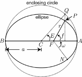
Figure 1: Variables describing the elliptical orbit. Figure reproduced from Ref. lvpn .

The standard keplerian characterization of an elliptical orbit is used in the orbital analysis of binary-pulsar systems to follow. The conventions are those of Ref. lvpn . Here we present the essential definitions of the parameters describing the orbit, and set up a relevant coordinate system for the analysis.

Some quantities helpful in developing the definitions to follow are shown in Fig. 1. The focus of the ellipse is labeled F. The point P located a coordinate distance $\displaystyle r$ from the focus indicates the location of the pulsar at coordinate time $\displaystyle t$. The semimajor axis of length $\displaystyle a$ lies between points B and C and between points A and C. The angle AFP is the true anomaly denoted $\displaystyle f$. The eccentric anomaly $\displaystyle E$ is defined by the angle ACQ, where Q is located at the intersection of the enclosing circle and a line perpendicular to the major axis passing through P. The angle $\displaystyle\omega$ is from the line of ascending nodes FN to the major axis.

The analysis to follow makes use of the general solution of the elliptic two-body problem. The notation $\displaystyle n$ is used for the orbital frequency and the period is defined as usual $\displaystyle P_{b}=2\pi/n$. The solution is generally characterized by six constants known as orbital elements: the semimajor axis $\displaystyle a$, the eccentricity $\displaystyle e$, the inclination of the orbit $\displaystyle i$, the longitude of the ascending node $\displaystyle\Omega$, the angle $\displaystyle\omega$ introduced above, and the mean anomaly $\displaystyle l_{0}$ at the epoch $\displaystyle t=t_{0}$ related to the eccentric anomaly $\displaystyle E$ via

$$E-e\sin E=l_{0}+n(t-t_{0}).$$ (10)

Further details can be found in Refs. lvpn ; osc .

Figure 2: Elliptical orbits in the post-Newtonian frame of the binary pulsar. Figure reproduced from Ref. lvpn .

The orbital elements $\displaystyle i$, $\displaystyle\Omega$, $\displaystyle\omega$ specify the orientation of the orbit in the reference coordinate system as shown in Fig. 2. It is also convenient to define a set of unit vectors that specify the orientation of the orbit. A typical choice defines $\displaystyle\vec{k}$ normal to the plane of the orbit, $\displaystyle\vec{P}$ pointing from the focus to the periastron, and $\displaystyle\vec{Q}=\vec{k}\times\vec{P}$. The relation between these vectors and the basis of the reference coordinate system $\displaystyle{\bf e}_{j}$ is then

$$\displaystyle\vec{P} \displaystyle= \displaystyle(\cos\Omega\cos\omega-\cos i\sin\Omega\sin\omega)\vec{e}_{1}$$

$$\displaystyle+(\sin\Omega\cos\omega+\cos i\cos\Omega\sin\omega)\vec{e}_{2}$$

$$\displaystyle+\sin i\sin\omega\vec{e}_{3},$$

$$\displaystyle\vec{Q} \displaystyle= \displaystyle-(\cos\Omega\sin\omega+\cos i\sin\Omega\cos\omega)\vec{e}_{1}$$

$$\displaystyle+(\cos i\cos\Omega\cos\omega-\sin\Omega\sin\omega)\vec{e}_{2}$$

$$\displaystyle+\sin i\cos\omega\vec{e}_{3},$$

$$\displaystyle\vec{k} \displaystyle= \displaystyle\sin i\sin\Omega\vec{e}_{1}-\sin i\cos\Omega\vec{e}_{2}$$ (11)

$$\displaystyle+\cos i\vec{e}_{3}.$$

With these definitions, the unperturbed orbit can be written

$$\displaystyle\vec{r} \displaystyle= \displaystyle{{a(1-e^{2})}\over{1+e\cos f}}(\vec{P}\cos f+\vec{Q}\sin f).$$ (12)

III Secular Changes

Nonzero coefficients for Lorentz violation $\displaystyle(\bar{a}_{\rm{eff}})_{\mu}$ and $\displaystyle\bar{c}_{\mu v}$ affect the pulsar and the companion’s relative motion and therefore modify the original Newtonian elliptical orbit. This section characterizes these effects by obtaining the secular changes in the six orbital elements $\displaystyle a,e,l_{0},i,\Omega,\omega$ generated by the coefficients for Lorentz violation.

To proceed, we adopted the method of osculating elements lvpn ; osc , which is a standard method that treats the relative motion of the pulsar and its companion as instantaneously part of an unperturbed elliptical orbit. Here this unperturbed orbit solves the equation

$${{d^{2}r^{j}}\over{dt^{2}}}=-{{GM\lambda}\over{r^{3}}}r^{j},$$ (13)

where

$$\displaystyle\lambda=1+{{1}\over{M}}\sum_{w}n_{1}^{w}m^{w}\overline{c}{}^{w}_{00}+{{2}\over{M}}\sum_{w}n_{3}^{w}\left(\bar{a}^{w}_{\rm eff}\right)_{0}.$$ (14)

The relation between the orbital frequency $\displaystyle n$ and the semimajor axis $\displaystyle a$ then takes the form

$$n^{2}a^{3}=GM\lambda.$$ (15)

Note that the combination of coefficients $\displaystyle\lambda$ appears as an effective contribution to $\displaystyle GM$ and is unobservable via the analysis of a single system.

Perturbations to the orbit are then characterized by a gradual time-evolution of the ellipse, with the six orbital elements now being functions of time. The perturbing acceleration can now be defined as the difference between the full modified acceleration (8) and the central acceleration (13). The result takes the form

$$\displaystyle\mathrm{a}^{\prime j}={{d^{2}r^{j}}\over{dt^{2}}}-{{d^{2}r^{j}_{0}}\over{dt^{2}}}={{G}\over{r^{2}}}\Big{(}A^{j}_{\phantom{j}l}\hat{r}^{l}+B^{j}v_{l}\hat{r}^{l}+C^{k}v_{k}\hat{r}^{j}$$

$$\displaystyle+{{1}\over{2}}(B^{k}+C^{k})\hat{r}_{k}v^{j}\Big{)},$$ (16)

where we classify the combinations of $\displaystyle(\overline{a}{}_{\rm{eff}})_{\mu}$ and $\displaystyle\overline{c}{}_{\mu\nu}$ into 3 kinds, namely $\displaystyle A^{j}_{\phantom{j}l}$, $\displaystyle B^{j}$, and $\displaystyle C^{j}$, according to their relations with $\displaystyle\vec{v}$ and $\displaystyle\vec{r}$ in (8). Specifically,

$$\displaystyle A^{j}_{\phantom{j}l} \displaystyle= \displaystyle\sum_{w}2\eta^{jk}n_{7}^{w}m^{w}\overline{c}{}^{w}_{\left(kl\right)}$$

$$\displaystyle B^{j} \displaystyle= \displaystyle-\sum_{w}2\eta^{jk}\Big{(}n_{2}^{w}\alpha\left(\bar{a}_{\rm eff}^{w}\right)_{k}$$

$$\displaystyle+\left(n_{6}^{w}-2n_{8}^{w}\right)m^{w}\overline{c}{}^{w}_{\left(0k\right)}\Big{)}$$

$$\displaystyle C^{j} \displaystyle= \displaystyle\sum_{w}2\eta^{jk}\Big{(}n_{2}^{w}\alpha\left(\bar{a}_{\rm eff}^{w}\right)_{k}+n_{6}^{w}m^{w}\overline{c}{}^{w}_{\left(0k\right)}\Big{)}.$$ (17)

Following the method of osculating elements osc then requires the following steps. The relative position $\displaystyle\vec{r}$ from Eq. (12) along with its coordinate-time derivative $\displaystyle\vec{v}$ are inserted into the perturbing acceleration (16). The relevant projections of the perturbing acceleration are then used to extract the variations in the orbital elements. The variations are averaged over an orbit via integration over the true anomaly $\displaystyle f$. For the secular variation in the semimajor axis and the eccentricity we find

$$\displaystyle\Big{\langle}{{da}\over{dt}}\Big{\rangle} \displaystyle= \displaystyle 0$$

$$\displaystyle\Big{\langle}{{de}\over{dt}}\Big{\rangle} \displaystyle= \displaystyle{{n}\over{M}}\left(1-e^{2}\right)^{1/2}\Big{(}{{e^{2}-2\varepsilon}\over{e^{3}}}A_{PQ}+{{na\varepsilon}\over{e^{2}}}B_{P}\Big{)},\phantom{aa}$$ (18)

where $\displaystyle\varepsilon=1-(1-e^{2})^{1/2}$ is the eccentricity function. The secular changes in the orbital elements related to the orientation of the ellipse are given by

$$\displaystyle\Big{\langle}{{di}\over{dt}}\Big{\rangle}= \displaystyle{{n}\over{M\left(1-e^{2}\right)^{1/2}}}\Big{(}{{\varepsilon}\over{e^{2}}}A_{kP}\cos\omega-{{e^{2}-\varepsilon}\over{e^{2}}}A_{kQ}\sin\omega$$

$$\displaystyle-{{n\varepsilon a}\over{e}}B_{k}\sin\omega\Big{)}$$

$$\displaystyle\Big{\langle}{{d\Omega}\over{dt}}\Big{\rangle}= \displaystyle{{n\sin i}\over{M\left(1-e^{2}\right)^{1/2}}}\Big{(}{{\varepsilon}\over{e^{2}}}A_{kP}\sin\omega+{{e^{2}-\varepsilon}\over{e^{2}}}A_{kQ}\cos\omega$$

$$\displaystyle+{{n\varepsilon a}\over{e}}B_{k}\cos\omega\Big{)}$$

$$\displaystyle\Big{\langle}{{d\omega}\over{dt}}\Big{\rangle}= \displaystyle-{{n}\over{M\tan i\left(1-e^{2}\right)^{1/2}}}\Big{(}{{\varepsilon}\over{e^{2}}}A_{kP}\sin\omega+$$ (19)

$$\displaystyle{{e^{2}-\varepsilon}\over{e^{2}}}A_{kQ}\cos\omega+{{n\varepsilon a}\over{e}}B_{k}\cos\omega\Big{)}$$

$$\displaystyle+{{n}\over{M}}\Big{[}{{e^{2}-2\varepsilon}\over{2e^{4}}}\left(A_{QQ}-A_{PP}\right)$$

$$\displaystyle\phantom{+{{n}\over{M}}\Big{[}}+{{na\left(e^{2}-\varepsilon\right)}\over{e^{3}\left(1-e^{2}\right)^{1/2}}}B_{Q}\Big{]},$$

while secular evolution of the mean anomaly at the epoch takes the form

$$\displaystyle\Big{\langle}{{dl_{0}}\over{dt}}\Big{\rangle} \displaystyle= \displaystyle-{{n}\over{M}}\Big{[}{{(e^{2}-2\varepsilon)\left(1-e^{2}\right)^{1/2}}\over{2e^{4}}}\left(A_{QQ}-A_{PP}\right)$$ (20)

$$\displaystyle+{{na\left(e^{2}-\varepsilon\right)}\over{e^{3}}}B_{Q}+{{2\varepsilon}\over{e^{2}}}A_{PP}+{{2(e^{2}-\varepsilon)}\over{e^{2}}}A_{QQ}$$

$$\displaystyle+{{3na\varepsilon}\over{e}}\left(B_{Q}+C_{Q}\right)\Big{]}.$$

Notice that these results are not limited to binary-pulsar systems but could be applied in any two-body celestial system. The application of these results to searches for Lorentz violation in binary pulsars is considered in the following sections.

Before concluding our development of secular changes in pulsar systems, we note that secular changes in the spin of solitary pulsars also arises in the presence of matter-sector coefficients for Lorentz violation. The effect can be attributed to the violations of angular-momentum conservation that accompany Lorentz violation. Following the derivation in Ref. Spin , we find

$$\Omega_{k}^{prec}=-{{2\pi}\over{mP}}\sum_{w}N^{w}m^{w}\overline{c}{}^{w}_{jk}\hat{S}^{j}$$ (21)

for the spin-precession frequency of a solitary pulsar at second post-Newtonian order. Here $\displaystyle P$ is the spin period, $\displaystyle m$ is the mass of the spinning body, and $\displaystyle\hat{S}$ is the unit vector pointing along the spin direction. Since spin precession can also be extracted from the pulse data, it is then also possible to measure the matter-sector coefficients for Lorentz violation in the context of solitary pulsars as well as other spinning bodies. This idea has already been used in the context of searches for changes in the magnitude of the angular velocity of pulsars to place constraints on combinations of $\displaystyle(\overline{c}{}^{n})_{jk}$ brettpuls .

IV Timing formula

The secular changes in the orbit of the pulsar system are observable through the rate at which pulses are received at Earth. To complete the prediction, the secular changes in the nature of the orbit should be combined with other curved-spacetime effects on the pulse rate. Here we consider such effects in developing a timing formula to be used in conjunction with the orbital elements above.

We begin by considering the trajectory of a photon traveling from the pulsar to Earth. The trajectory is determined by the null condition $\displaystyle ds^{2}=0$ where the relevant metric is obtained from (6). The same simplifications used in the gravity sector lvpn hold here. Time-delay effects associated with the pulsar itself can be disregarded in this analysis since they result in a constant shift. Time-delay effects from the companion, which could be obtained via the general analysis of time delay in the matter sector lvgap , are negligibly small in the present context. Effects of solar-system bodies and the motion of the detector are omitted for simplicity. With this, the photon trajectory reduces to the simple relation

$$t_{\rm arr}-t_{\rm em}=|\vec{r}_{E}-\vec{r}_{1}|,$$ (22)

where $\displaystyle\vec{r}_{E}$ is the location of Earth, $\displaystyle t_{\rm em}$ is the coordinate time of emission by the pulsar, and $\displaystyle t_{\rm arr}$ is the coordinate time of arrival at Earth.

Contact must then be made with the proper time of emission. This can be done through consideration of the relation between the proper-time interval measured by an ideal clock at the surface of the pulsar and the coordinate-time interval obtained from the metric (6)

$$\displaystyle d\tau=dt[1-kU-{\textstyle{1\over 2}}\vec{v}_{1}^{2}].$$ (23)

Here $\displaystyle\vec{v}_{1}$ is the velocity of the pulsar. The potential in (23) includes contributions from both the pulsar and its companion evaluated along the trajectory of the clock $\displaystyle U={{Gm_{2}}\over{r}}+U_{1}$. The contribution $\displaystyle U_{1}$ from the pulsar generates an unobservable constant shift and will be neglected in what follows. As a result, $\displaystyle k$ can be taken as the isotropic combination of SME coefficients

$$\displaystyle k=1+{{1}\over{m_{2}}}\sum_{w}N_{2}^{w}m^{w}\overline{c}{}^{w}_{00}+{{2}\over{m_{2}}}\sum_{w}N_{2}^{w}\left(\bar{a}_{\rm eff}^{w}\right)_{0}.$$ (24)

The velocity of the pulsar $\displaystyle\vec{v}_{1}$ can be obtained from the relative velocity $\displaystyle\vec{v}$ through the modified version of conservation of momentum at second post-Newtonian order along with our coordinate choices. The total momentum of the system takes the form

$$\displaystyle(p_{\rm Tot})_{j} \displaystyle= \displaystyle m_{1}(\delta_{jk}+\overline{c}{}^{1}_{00}\delta_{jk}+2\bar{c}^{1}_{jk})(v_{1})_{k}$$ (25)

$$\displaystyle+m_{2}(\delta_{jk}+\overline{c}{}^{2}_{00}\delta_{jk}+2\bar{c}^{2}_{jk})(v_{2})_{k}$$

$$\displaystyle+(p_{a})_{j}+(p_{c})_{j}+(p_{s})_{j}+\ldots,$$

where a superscript $\displaystyle 1$ indicates the coefficients for the pulsar and $\displaystyle 2$ indicates the coefficients for its companion, which can be expanded in terms of the species content of the bodies via Eq. (5). The additional terms

$$\displaystyle(p_{a})_{j} \displaystyle= \displaystyle{{2G\alpha}\over{r}}\left(m_{1}(\overline{a}{}^{2}_{\rm{eff}})_{j}+m_{2}(\overline{a}{}^{1}_{\rm{eff}})_{j}\right)$$

$$\displaystyle(p_{c})_{j} \displaystyle= \displaystyle{{m_{1}m_{2}^{2}}\over{M^{2}}}\left(\overline{c}{}^{1}_{0j}v^{2}+2\overline{c}{}^{1}_{0k}v_{k}v_{j}\right)+{{2Gm_{1}m_{2}}\over{r}}\overline{c}{}^{1}_{0j}$$ (26)

$$\displaystyle+(1\leftrightarrow 2)$$

denote contributions at post-Newtonian order three that are relevant for our subsequent analysis. We note in passing that a similar order three contribution exists associated with gravity-sector coefficient $\displaystyle\overline{s}{}^{\mu\nu}$:

$$(p_{s})_{j}={{Gm_{1}m_{2}}\over{r}}\left(3\overline{s}{}_{0j}+\overline{s}{}_{0k}\hat{r}_{k}\hat{r}_{j}\right).$$ (27)

Our choice of frame is fixed by the condition $\displaystyle(p_{\rm Tot})_{j}=0$.

We then integrate (23) to obtain the desired relation between the coordinate time of emission and the proper time of emission. The integration is facilitated by a change variables from coordinate time to the eccentric anomaly $\displaystyle E$, which is related to the true anomaly $\displaystyle f$ by

$$\displaystyle\tan{{f}\over{2}}=\left({{1+e}\over{1-e}}\right)^{1/2}\tan{{E}\over{2}}.$$ (28)

Replacing $\displaystyle r$ in (23) using (12) along with (28), we can then perform integration over $\displaystyle E$, which yields, up to constants,

$$\displaystyle\tau= \displaystyle\hskip-8.0ptt-{{kGm_{2}P_{b}}\over{2\pi a}}E-{{\lambda Gm_{2}^{2}P_{b}}\over{2M\pi a}}E-\sum_{w}{{Gm_{1}m_{2}m^{w}n_{4}^{w}P_{b}}\over{M^{2}\pi a}}$$ (29)

$$\displaystyle\times\Big{[}{{m_{2}\overline{c}{}^{w}_{00}}\over{M}}E-2{{\overline{c}{}^{w}_{PP}-\left(1-e^{2}\right)\overline{c}{}^{w}_{QQ}}\over{e^{2}}}E$$

$$\displaystyle+\left(\overline{c}{}^{w}_{PP}-\overline{c}{}^{w}_{QQ}\right)\mathcal{K}_{1}\left(E\right)-\overline{c}{}^{w}_{PQ}\mathcal{K}_{2}\left(E\right)\Big{]}.$$

Subscripts $\displaystyle P$, $\displaystyle Q$ and $\displaystyle k$ on the coefficients for Lorentz violation indicate projections along the directions $\displaystyle\vec{P}$ , $\displaystyle\vec{Q}$ and $\displaystyle\vec{k}$. For example, $\displaystyle\overline{c}{}^{w}_{P}=-\overline{c}{}^{w}_{0j}P_{j}$. The functions $\displaystyle\mathcal{K}_{1}$ and $\displaystyle\mathcal{K}_{2}$ appearing in (14) are given by

$$\displaystyle\mathcal{K}_{1}\left(E\right) \displaystyle= \displaystyle{{2\left(1-e^{2}\right)^{1/2}}\over{e^{2}}}\arctan\left[\left({{1+e}\over{1-e}}\right)^{1/2}\tan{\textstyle{{1}\over{2}}}E\right]$$

$$\displaystyle\mathcal{K}_{2}\left(E\right) \displaystyle= \displaystyle{{2\left(1-e^{2}\right)^{1/2}}\over{e^{2}}}\Big{[}e\cos E+\ln\left(1-e\cos E\right)\Big{]}.$$ (30)

The constant in Eq. (10) is fixed via the choice $\displaystyle E-e\sin E=n(t_{\rm arr}-r_{E})$.

The desired relation between the proper time of emission and the time of arrival is then obtained by combining Eq. (29) with Eq. (22) yielding

$$\displaystyle\tau \displaystyle= \displaystyle t_{\rm arr}-{\cal A}(\cos E-e)-{\cal B}\sin E$$ (31)

$$\displaystyle-{{2\pi aa_{1}e}\over{P_{b}}}\left(k+{\textstyle{{m_{2}}\over{M}}}\lambda\right)\sin E$$

$$\displaystyle-{{2\pi}\over{P_{b}}}{{({\cal A}\sin E-{\cal B}\cos E)}\over{(1-e\cos E)}}[{\cal A}(\cos E-e)+{\cal B}\sin E]$$

$$\displaystyle-\sum_{w}{{Gm_{1}m_{2}m^{w}n_{4}^{w}P_{b}}\over{M^{2}\pi a}}\Big{[}{{em_{2}\overline{c}{}^{w}_{00}}\over{M}}\sin E$$

$$\displaystyle-2{{\overline{c}{}^{w}_{PP}-\left(1-e^{2}\right)\overline{c}{}^{w}_{QQ}}\over{e}}\sin E+\left(\overline{c}{}^{w}_{PP}-\overline{c}{}^{w}_{QQ}\right){\cal K}_{1}(E)$$

$$\displaystyle-\overline{c}{}^{w}_{PQ}{\cal K}_{2}(E)\Big{]}+\tau_{{\rm CM}a}+\tau_{{\rm CM}c}.$$

Here $\displaystyle{\cal A}$ and $\displaystyle{\cal B}$ are the combinations

$$\displaystyle{\cal A} \displaystyle= \displaystyle a_{1}\sin i\sin\omega,$$

$$\displaystyle{\cal B} \displaystyle= \displaystyle\sqrt{(1-e^{2})}~{}a_{1}\sin i\cos\omega,$$ (32)

and $\displaystyle a_{1}=am_{2}/M$. Note that with the exception of Eq. (3), the coefficients for Lorentz violation $\displaystyle a_{\mu}$ appears in the combination $\displaystyle(a_{\rm{eff}})_{\mu}$ throughout this work. Hence conflict between these two standard uses of a lower index on an object $\displaystyle a$ is avoided. In obtaining Eq. (31), our choice of origin as the modified center of mass is used to fix $\displaystyle\vec{r}_{1}$. Explicitly our choice corresponds to the requirement

$$\int(p_{\rm Tot})_{j}dt=0.$$ (33)

The contributions $\displaystyle\tau_{{\rm CM}a}$ and $\displaystyle\tau_{{\rm CM}c}$ are a result of the Lorentz violating contributions to the momentum associated with the $\displaystyle(\overline{a}{}_{\rm{eff}})_{\mu}$ and $\displaystyle\overline{c}{}_{\mu\nu}$ coefficients respectively. The contribution associated with $\displaystyle(\overline{a}{}_{\rm{eff}})_{\mu}$ takes the form

$$\displaystyle\tau_{{\rm CM}a} \displaystyle= \displaystyle-{{4\pi ae}\over{P_{b}m_{2}}}\sum_{w}n^{w}_{5}\alpha\sin E\Big{[}(a^{w}_{\rm{eff}})_{P}{\cal A}$$

$$\displaystyle\hskip 20.0pt+(a^{w}_{\rm{eff}})_{Q}{{{\cal B}}\over{\sqrt{1-e^{2}}}}+(a^{w}_{\rm{eff}})_{k}a_{1}\cos\omega\Big{]},$$

while $\displaystyle\overline{c}{}_{\mu\nu}$ contributes

$$\displaystyle\tau_{{\rm CM}c}\hskip-8.0pt \displaystyle=-\sum_{w}{{2m_{1}m^{w}n^{w}_{4}}\over{M^{2}}}[\Xi^{w}(\cos E-e)+\Sigma^{w}\sin E]$$ (35)

$$\displaystyle-\sum_{w}{{4\pi m_{1}m^{w}n^{w}_{4}}\over{P_{b}M^{2}}}$$

$$\displaystyle\times\Big{[}{{{\cal A}(\cos E-e)+{\cal B}\sin E}\over{1-e\cos E}}\left(\Xi^{w}\sin E-\Sigma^{w}\cos E\right)$$

$$\displaystyle\hskip 5.0pt+{{{\cal A}\sin E-{\cal B}\cos E}\over{1-e\cos E}}\left(\Xi^{w}(\cos E-e)+\Sigma^{w}\sin E\right)\Big{]}$$

$$\displaystyle+\sum_{w}{{4\pi am_{1}m^{w}}\over{P_{b}M^{2}}}\Big{[}(n^{w}_{3}+2n^{w}_{7})\Upsilon^{w}e\sin E$$

$$\displaystyle\hskip 5.0pt+{\textstyle{1\over 2}}n^{w}_{7}\Big{(}\overline{c}{}^{w}_{Q}{\cal A}+\overline{c}{}^{w}_{p}{{{\cal B}}\over{\sqrt{1-e^{2}}}}\Big{)}{\cal K}_{2}(E)$$

$$\displaystyle\hskip 5.0pt+n^{w}_{7}\Big{(}\overline{c}{}^{w}_{P}{\cal A}-\overline{c}{}^{w}_{Q}{{{\cal B}}\over{\sqrt{1-e^{2}}}}\Big{)}({\cal K}_{1}(E)-{\textstyle{{2}\over{e}}}\sin E)\Big{]}.$$

Here $\displaystyle\Xi^{w}$ and $\displaystyle\Sigma^{w}$ are defined as

$$\displaystyle\Xi^{w} \displaystyle= \displaystyle({\textstyle{1\over 2}}\overline{c}{}^{w}_{00}+\overline{c}{}^{w}_{PP}){\cal A}+\overline{c}{}^{w}_{PQ}{{{\cal B}}\over{\sqrt{1-e^{2}}}}+\overline{c}{}^{w}_{Pk}a_{1}\cos i$$

$$\displaystyle\Sigma^{w} \displaystyle= \displaystyle\overline{c}{}^{w}_{QP}{\cal A}\sqrt{1-e^{2}}+({\textstyle{1\over 2}}\overline{c}{}^{w}_{00}+\overline{c}{}^{w}_{QQ}){\cal B}+\overline{c}{}^{w}_{Qk}a_{1}\cos i$$

$$\displaystyle\Upsilon^{w} \displaystyle= \displaystyle\overline{c}{}^{w}_{P}{\cal A}+\overline{c}{}^{w}_{Q}{{{\cal B}}\over{\sqrt{1-e^{2}}}}+\overline{c}{}^{w}_{k}a_{1}\cos i.$$ (36)

We note that the result of including this effect in the gravity sector would generate the additional contribution

$$\displaystyle\tau_{{\rm CM}s} \displaystyle= \displaystyle-{{2\pi am_{1}}\over{P_{b}M}}\Big{[}3e\overline{s}{}_{k}a_{1}\cos i\sin E$$ (37)

$$\displaystyle+\overline{s}{}_{P}\Big{(}{\cal A}{{(1+3e^{2})\sin E}\over{e}}+{\cal A}{\cal F}_{1}(E)+{\cal B}{\cal F}_{2}(E)\Big{)}$$

$$\displaystyle-{{\overline{s}{}_{Q}}\over{\sqrt{1-e^{2}}}}\Big{(}{\cal B}{{(1-4e^{2})\sin E}\over{e}}-{\cal B}{\cal F}_{1}(E)$$

$$\displaystyle\phantom{-{{\overline{s}{}_{Q}}\over{\sqrt{1-e^{2}}}}\Big{(}}-(1-e^{2}){\cal A}{\cal F}_{2}(E)\Big{)}\Big{]}$$

in the arrival time relation for the gravity sector, Eq. (180) of Ref. lvpn . The functions $\displaystyle{\cal F}_{1}(E)$ and $\displaystyle{\cal F}_{2}(E)$ are provided as Eq. (178) of Ref. lvpn .

The results of this section, used in conjunction with the evolution of the orbital elements could then be used to search for matter-sector Lorentz violation in pulsar timing data. A direct search could be done by inserting Eq. (31) into a model for the emission of pulses as a function of the proper time at the surface of the pulsar $\displaystyle\tau$. This would provide an equation for the received pulses as a function of arrival time that could be fit to the observational data. Limits can also be placed through the statistical analysis of existing fits to a number of pulsar systems shao , such as fits performed in the parametrized post-Keplerian formalism ppk .

Crude estimates of the sensitivities that might be obtained via pulsar systems can be seen by comparing the results of Shao’s recent analysis of the pure-gravity sector shao with existing sensitivities to $\displaystyle(\overline{a}{}_{\rm{eff}})_{\mu}$ and $\displaystyle\overline{c}{}_{\mu\nu}$ data . For example, Shao finds sensitivity to $\displaystyle\overline{s}{}^{TJ}$ at the $\displaystyle 10^{-8}$ level. Based on the similarity in the equations, sensitivity to $\displaystyle(\overline{a}{}_{\rm{eff}})_{J}$ at a similar level might be expected, which would amount to an improvement of about 3 orders of magnitude over existing constraints. It should also be emphasized that in the matter sector, different systems having different compositions offer different sensitivities. For example, a neutron star-white dwarf system is sensitive to a different linear combination of coefficients than a double neutron star system. If the existence of more exotic stars is confirmed, such as strange stars, these systems may offer unique sensitivities to the associated coefficients. The prospects noted here are likely to be further enhanced by anticipated observational improvements in the coming years.

V Summary

In this work we have derived the effects of matter-sector Lorentz violation on both the motion of binary-pulsar systems and the pulses traveling from them via a post-Newtonian treatment. The Lorentz-violating corrections to the relative motion of the pulsar and companion are developed in Sec. III via the method of osculating elements. Equations (18)-(20) provided the secular changes to the orbital elements resulting from this analysis. These results can then be used in conjunction with the modifications to the timing formula developed in Sec. IV, where the central result is the relation between the proper time of pulse emission and the time of arrival (31). In obtaining this result, we consider the effects of Lorentz-violating corrections to the conserved momentum (25) in pulsar systems.

Analysis of existing pulsar-timing data using the results presented here will provide the first consideration of Lorentz violation in matter-gravity couplings in strong-gravity systems, and will yield significant sensitivity improvements over existing solar system and laboratory sensitivities. Matter-sector Lorentz violation is in general accompanied by particle-species dependent effects, making measurements in systems involving different types of bodies of significant interest. The use of existing data can provided about 3 orders of magnitude improvement over existing measurements from other systems. Going forward, prospects for additional improvement via observational advances are excellent.

References

- (1) A. Hewish, S.J. Bell, J.D.H. Pilkington, P.F. Scott, and R.A. Collins, R.A., Nature 217, 709 (1968).
- (2) R.A. Hulse and J.H. Taylor, Astrophys. J. 195, L51 (1975).
- (3) For reviews, see I.H. Stairs, Living Rev. Relativity 6, 5 (2003); R.N. Manchester, Int. J. Mod. Phys. D 24, 1530018 (2015).
- (4) For recent reviews, see J.D. Tasson, Rep. Prog. Phys. 77, 062901 (2014), S. Liberati, Class. Quant. Grav. 30 133001 (2013).
- (5) V.A. Kostelecký and S. Samuel, Phys. Rev. D 39, 683 (1989).
- (6) D. Colladay and V.A. Kostelecký, Phys. Rev. D 55, 6760 (1997); Phys. Rev. D 58, 116002 (1998).
- (7) V.A. Kostelecký, Phys. Rev. D 69, 105009 (2004).
- (8) Q.G. Bailey and V.A. Kostelecký, Phys. Rev. D 74, 045001 (2006).
- (9) M.D. Seifert, Phys. Rev. D 79, 124012 (2009); Phys. Rev. D 81, 065010 (2010); B. Altschul, Q.G. Bailey, and V.A. Kostelecký, Phys. Rev. D 81, 065028 (2010); Q.G. Bailey and R. Tso, Phys. Rev. D 84, 085025 (2011); Y. Bonder, Phys. Rev. D 91, 125002 (2015).
- (10) L. Shao, Phys. Rev. D 90, 122009 (2014); Phys. Rev. Lett. 112, 111103 (2014).
- (11) A. Hees, Q.G. Bailey, C. Le Poncin-Lafitte, A. Bourgoin, A. Rivoldini, B. Lamine, F. Meynadier, C. Guerlin, and P. Wolf, arXiv:1508.03478.
- (12) J.B.R. Battat, J.F. Chandler, and C.W. Stubbs, Phys. Rev. Lett. 99, 241103 (2007); H. Müller et al., Phys. Rev. Lett. 100, 031101 (2008); K.-Y. Chung et al., Phys. Rev. D 80, 016002 (2009); D. Bennett, V. Skavysh, and J. Long, in V.A. Kostelecký, ed., CPT and Lorentz Symmetry V, World Scientific, Singapore 2011; L. Iorio, Class. Quant. Grav. 29, 175007 (2012); Q.G. Bailey, R.D. Everett, and J.M. Overduin, Phys. Rev. D 88, 102001 (2013).
- (13) Q. Bailey, V.A. Kostelecký, and R. Xu, Phys. Rev. D 91, 022006 (2015); V.A. Kostelecký and J.D. Tasson, Phys. Lett. B 749, 551 (2015).
- (14) J.C. Long and V.A. Kostelecký, Phys. Rev. D 91, 092003 (2015); C.-G. Shao, Y.-J. Tan, W.-H. Tan, S.-Q. Yang, J. Luo, and M.E. Tobar, Phys. Rev. D 91, 102007 (2015); C.-G. Shao et al., in preparation.
- (15) V.A. Kostelecký, and J.D. Tasson, Phys. Rev. D 83, 016013 (2011).
- (16) V.A. Kostelecký, and J.D. Tasson, Phys. Rev. Lett. 102, 010402 (2009).
- (17) H. Panjwani, L. Carbone, and C.C. Speake, in V.A. Kostelecký, ed., CPT and Lorentz Symmetry V, World Scientific, Singapore, 2011; J.D. Tasson, Phys. Rev. D 86, 124021 (2012); M.A. Hohensee, H. Müller, and R.B. Wiringa, Phys. Rev. Lett. 111, 151102 (2013); M.A. Hohensee et al., Phys. Rev. Lett. 106, 151102 (2011).
- (18) Data Tables for Lorentz and CPT Violation, V.A. Kostelecký and N. Russell, 2015 edition, arXiv:0801.0287v8.
- (19) B. Altschul, Phys. Rev. D 75, 023001 (2007).
- (20) Y. Xie, Res. Astron. Astrophys. 13, 1 (2013).
- (21) G. Lambiase, Phys. Rev. D 71 065005 (2005).
- (22) C.M. Will, Living Rev. Relativity 17, 4 (2014); T. Damour and G. Esposito-Farèse, Class. Quantum Grav. 9, 2093 (1992); I.H. Stairs, et al., ApJ 632, 1060 (2005); L. Shao and N. Wex, Class. Quantum Grav. 29, 215018 (2012); L. Shao et al., Class. Quantum Grav. 30, 165019 (2013); B.Z. Foster, Phys. Rev. D 76, 084033 (2007); N. Wex and M. Kramer, Mon. Not. R. Astron. Soc. 380, 455 (2007).
- (23) J.H. Taylor, L.A. Fowler, and P.M. McCulloch, Nature 277, 437 (1979); J.M. Weisberg, D.J. Nice, and J.H. Taylor, Astrophys. J. 722, 1030 (2010).
- (24) K. Yagi, D. Blas, N. Yunes, and E. Barausse, Phys. Rev. Lett. 112, 161101 (2014).
- (25) L. Shao, et al., PoS AASKA14 042 (2014).
- (26) C.M. Will, Theory and Experiment in Gravitational Physics, Cambridge University Press, Cambridge, England, 1993.
- (27) R. Bluhm, Phys. Rev. D 91, 065034 (2015).
- (28) V.A. Brumberg, Essential Relativistic Celestial Mechanics. Adam Hilger, London (1991).
- (29) K. Nordtvedt, Astrophys. J. 320, 871 (1987).
- (30) T. Damour and J.H. Taylor, Phys. Rev. D 45, 1840 (1992).