Formulae in noncommutative Hodge theory
Abstract
Abstract: We prove that the cyclic homology of a saturated category admits the structure of a ‘polarized variation of Hodge structures’, building heavily on the work of many authors: the main point of the paper is to present complete proofs, and also explicit formulae for all of the relevant structures. This forms part of a project of Ganatra, Perutz and the author, to prove that homological mirror symmetry implies enumerative mirror symmetry.
1 Introduction
1.1 Calabi–Yau mirror symmetry
Mirror symmetry predicts the existence of certain ‘mirror’ pairs of Calabi–Yau Kähler manifolds, and , so that the Gromov–Witten invariants of can be extracted from certain Hodge-theoretic invariants of .111We only consider genus-zero Gromov–Witten invariants in this paper. The first thrilling application of mirror symmetry was the prediction of the number of rational curves, in all degrees, on the quintic threefold , in terms of the Hodge theory of a mirror manifold [CdlOGP91]. This prediction for the quintic, together with many more examples of mirror symmetry, was later mathematically verified [Giv96, LLY97].
The most conceptually satisfying way of formulating the mirror relationship between numerical invariants of and is as an isomorphism of variations of Hodge structures () [Mor93]. A over a complex manifold consists of a holomorphic vector bundle , equipped with a filtration by holomorphic subbundles, and a flat connection satisfying the condition known as Griffiths transverality.222This is more precisely referred to as a complex variation of Hodge structures. We introduce the Kähler moduli space , which parametrizes deformations of the Kähler form on , and the complex moduli space , which parametrizes deformations of the complex structure on . The Gromov–Witten theory of gets packaged into the -model , which lives over the Kähler moduli space: . The Hodge theory on deformations of gets packaged into the -model , which lives over the complex moduli space: . Hodge-theoretic mirror symmetry then predicts an isomorphism , covering an isomorphism called the mirror map. Enumerative mirror symmetry, i.e., the explicit formulae relating the numerical invariants, can be deduced from this isomorphism of (see, e.g., [CK99]).
Kontsevich proposed a generalization of Hodge-theoretic mirror symmetry called homological mirror symmetry [Kon95]. It predicts a quasi-equivalence of categories , where is the split-closed derived Fukaya category of , and is a enhancement of the bounded derived category of coherent sheaves on . More precisely, one should think of these as families of categories, parametrized by the Kähler and complex moduli spaces respectively; and the quasi-equivalence matches the Fukaya category living over a point in Kähler moduli space with the derived category living over the corresponding point in complex moduli space, where the correspondence between moduli spaces is given by the same mirror map as before.
Kontsevich also predicted that homological should imply Hodge-theoretic mirror symmetry. This was subsequently made more precise [Bar02, KKP08, Cos09]. The expectation is that the cyclic homology of a family of saturated categories carries the structure of a ; the cyclic homology of the Fukaya category is isomorphic to ; and the cyclic homology of the bounded derived category of coherent sheaves is isomorphic to . Therefore, the equivalence of categories implies the isomorphism of .
This paper forms part of a project of the author, joint with Ganatra and Perutz, to carry out this program. Theorem 1.4 implies roughly that the cyclic homology of a family of saturated -graded categories carries the structure of a , and this structure is functorial under functors; we also give explicit formulae for all of the relevant structures. Ganatra [Gana] has defined a map from the cyclic homology of the Fukaya category to the -model ; this map is shown to respect the structure in [GPSa], using the formulae in the present paper; and the map is shown to be an isomorphism in [GPSb]. The corresponding comparison theorem for the -model is known to experts, although not everything is written in the literature; modulo this -model comparison theorem, the proof is complete.
We refer to [GPSb] for precise statements of the results. One corollary of them is a new proof of the mirror symmetry predictions for Gromov–Witten invariants of the quintic, as a consequence of the proof of homological mirror symmetry for the quintic [She15]. The -model comparison theorem has been established in this specific case by Tu [Tu].
1.2 Fano mirror symmetry
Although mirror symmetry was originally formulated for mirror pairs of Calabi–Yau Kähler manifolds , it admits a generalization in which is allowed to be Fano. In this case the mirror is no longer a manifold, but rather a ‘Landau–Ginzburg model’ , which means a variety equipped with a function . The Gromov–Witten invariants of are related to the singularity theory of [Giv95].
Once again, the relation between the numerical invariants can be expressed in terms of an isomorphism ; however, the structures getting identified are now variations of semi-infinite Hodge structures (). This notion was introduced by Barannikov [Bar01], but the study of the -model associated to goes back to Saito [Sai83].
In Section 2 we define the notion of a graded . The following notions are equivalent:
| -graded | |||
| -graded |
We refer to [GPSb, Lemma 2.7] for a precise statement and proof of the latter equivalence, which is a version of the ‘Rees correspondence’ between filtered bundles over and equivariant bundles over [Sim97]. Thus, Hodge-theoretic mirror symmetry can always be formulated as an isomorphism of graded ; in the Fano case the grading group is , and in the Calabi–Yau case it is . For the rest of the paper, ‘’ will always mean ‘graded ’, with the grading group implicit.
Homological mirror symmetry admits a generalization to the Fano case: roughly, it predicts a quasi-equivalence of -graded categories , where the latter is the category of matrix factorizations of [Orl04]. One expects that it should imply Hodge-theoretic mirror symmetry, by a similar argument to the Calabi–Yau case, but with replaced by .
Our Theorem 1.4 implies roughly that the cyclic homology of a family of saturated -graded categories, which satisfies the degeneration property, carries the structure of a -graded . The case is the one relevant to Fano mirror symmetry, and the case is the one relevant to Calabi–Yau mirror symmetry. In the latter case the degeneration property holds automatically, by Kaledin’s proof [Kal17] of Kontsevich–Soibelman’s degeneration conjecture [KS08, Conjecture 9.1.2]. In particular, our result implies that the cyclic homology of a family of saturated -graded categories carries the structure of a -graded , which we recall is equivalent to a (we stated this version of the result in the previous section). We remark that the grading group does not enter into the proof of Theorem 1.4: the cases of relevance to Fano and Calabi–Yau mirror symmetry are handled uniformly.
1.3 Standing notation
Let be fields. We will write , and .
We fix a grading group throughout: more precisely, we fix a ‘grading datum’ in the sense of [She15], which is an abelian group together with homomorphisms whose composition is non-zero. All of our structures are -graded; when we talk about an element of degree , we really mean its degree is the image of under the map ; and when we write a Koszul-type sign , it means that the image of the -degree of , under the map , is .
The two most relevant grading data are and ; working with the former is equivalent to working with ordinary -gradings, while working with the latter is equivalent to working with ordinary -gradings.
We define to be the graded ring of formal power series in a formal variable of degree , and the graded ring of formal Laurent series. For any or , we denote
To be precise, (respectively, ) is the degreewise completion of (respectively, ) with respect to the -adic filtration. If the morphism is not injective then this includes infinite sums of powers of , but if the morphism is injective then the completion has no effect because all powers of have different degrees. Thus contains ‘semi-infinite’ sums of powers of in the -graded case; hence Barannikov’s terminology.
Finally, if , we denote .
1.4 Main result
We define various flavours of in Section 2. To give an idea of what they mean, let us explain roughly what they correspond to under the Rees correspondence, in the -graded case:
-
•
An unpolarized pre- over corresponds to an -module equipped with a filtration and flat connection satisfying Griffiths transversality.
-
•
An unpolarized is an unpolarized pre- such that the -module is a finite-rank vector bundle.
-
•
A polarization for an unpolarized pre- is a covariantly constant pairing such that for , and for some called the weight; a polarized pre- is a pre- equipped with a polarization.
-
•
A polarized is a polarized pre-, such that the -module is a finite-rank vector bundle, and the pairing is non-degenerate.
Note that a polarized/unpolarized is the same thing as a polarized/unpolarized pre- satisfying additional properties, rather than equipped with additional data.
Our main results concern the Hochschild invariants of categories:
Let be a -linear graded category. Then:
-
1.
Its negative cyclic homology , endowed with the Getzler–Gauss–Manin connection [Get93], carries the structure of an unpolarized pre- over .
- 2.
-
3.
These structures are Morita invariant.
-
4.
If is saturated and its noncommutative Hodge-to-de Rham spectral sequence degenerates, then the polarized pre- is in fact a polarized .
A conjecture of Kontsevich and Soibelmann [KS08, Conjecture 9.1.2] says that the noncommutative Hodge-to-de Rham spectral sequence degenerates for any saturated . The conjecture has been proved by Kaledin in the case that is -graded [Kal17] (see also [Mat]); so far as the author is aware it remains open if is, for example, -graded.
Katzarkov–Kontsevich–Pantev conjecture that the of Theorem 1.4 can be endowed with a natural -structure (see [KKP08, Section 2.2.6], and also [Bla16]).
Let us comment on the originality of Theorem 1.4. We believe our contribution ranges from ‘writing down explicit formulae for known structures with uniform sign conventions, as a handy reference’ at the low end, to ‘checking that these structures have certain natural (but slightly tricky-to-prove) compatibilities’ at the high end. To be precise:
-
•
Our proof of the Morita invariance of the Getzler–Gauss–Manin connection is new.
-
•
Shklyarov’s construction of the higher residue pairing for categories [Shk16] immediately gives the construction for categories, because any category is quasi-equivalent to a category via the Yoneda embedding. On the other hand, for an category whose morphism spaces are finite-dimensional on the chain level, work of Costello [Cos07] and Konstevich–Soibelman [KS08] implies that there should be an explicit formula for the pairing. We write down the formula and prove that it is equivalent to Shklyarov’s definition (see Proposition 64). Our proof is motivated by Shklyarov’s [Shk16, Proposition 2.6].
-
•
Using the explicit formula for the higher residue pairing, we establish that it is covariantly constant with respect to the Getzler–Gauss–Manin connection: we believe that this result is also new (a related result was proven by Shklyarov in [Shk16], but that was for a different version of Getzler’s connection, namely the one in the -direction rather than in the direction of the base).
Now we give a guide, to help the reader find the proofs of the different parts of Theorem 1.4. Part (1) is proved in Section 3. Part (2) is proved in two parts: covariant constancy of the higher residue pairing, with respect to the Getzler–Gauss–Manin connection, is proved in Corollary 67; and symmetry of the higher residue pairing (which is the only part that requires the weak proper Calabi–Yau structure) is proved in Lemma 70. The tools to prove part (3) are developed in Section 4; Morita invariance of negative cyclic homology and the Getzler–Gauss–Manin connection are proved in Corollary 33, and Morita invariance of the higher residue pairing is proved in Proposition 62. Part (4) is proved in Theorem 72.
The paper involves a lot of long formulae composing multilinear operations in complicated ways, with non-trivial sign factors. We explain a graphical notation for these composition rules in Appendix C, which allows one to check various identities, with signs, in an efficient way; and we draw the graphical notation for some of the trickiest signs that appear in the paper. We omit the proofs of some identities that become trivial using the graphical notation, however we have tried very hard to write down explicitly the correct signs for every operation we define.
Acknowledgments.
I would like to thank Sheel Ganatra and Tim Perutz, my collaborators on the larger project of which this paper is a part (see [GPSb, PSa, PSb, GPSa]). The material in this paper was originally intended to form a background section to one of the papers in that series, but it turned out to be so long, and in such a different direction, that it made sense to split it off. Conversations with Ganatra and Perutz, and their suggestions, were extremely helpful in completing the paper. I am also very grateful to Paul Seidel for helpful conversations about the Mukai pairing. I thank Lino Amorim and Junwu Tu for pointing out some sign errors in a previous version. I thank the anonymous referee for helpful suggestions. While working on this project I was partially supported by the National Science Foundation through Grant number DMS-1310604, and under agreement number DMS-1128155. Any opinions, findings and conclusions or recommendations expressed in this material are those of the author and do not necessarily reflect the views of the National Science Foundation. I was also partially supported by a Royal Society University Research Fellowship. I am also grateful to the IAS and the Instituto Superior Técnico for hospitality while working on this project.
2 Variations of semi-infinite Hodge structures: definitions
Variations of semi-infinite Hodge structures () were introduced in [Bar01]. Here we recall the basic definitions, following [CIT09, Section 2.2] and [Gro11, Chapter 2]. We break with certain conventions in the literature, for which we apologize. We point out the places where our conventions differ as we go along.
Recall our standing notation: we fix a grading datum , and fields , and define , .
2.1 Pre-
Definition 1.
An unpolarized pre- over consists of a graded -module , equipped with a flat connection333More precisely, there is a map , such that is -linear in , additive in , satisfying (Leibniz rule) (flatness) of degree .
Definition 2.
A polarization for a pre- is a pairing
of degree , additive in both inputs, and satisfying
| (sesquilinearity) | ||||
| (covariant constance) | ||||
| (symmetry) |
where is called the weight.
It is not usually assumed that a polarization must have degree : we prefer to shift whatever pre- we are considering so that this is the case. In this paper, polarizations will arise from Shklyarov’s higher residue pairing on cyclic homology, which has degree with respect to the standard grading.
Definition 3.
A morphism of pre- is a degree- morphism of -modules which respects the connections, and, if the pre- are polarized, satisfies .
2.2
Definition 4.
An unpolarized is an unpolarized pre- such that is a free -module of finite rank.
Definition 5.
A polarization for a is a polarization for the underlying pre-, which is furthermore non-degenerate: i.e., the pairing of -vector spaces
induced by is non-degenerate.
A morphism of (polarized or unpolarized) is the same thing as a morphism of the underlying pre-.
What we call a ‘-graded polarized ’ is usually simply called a , in particular, the polarization is part of the structure. However, the notion of an unpolarized has applications in mirror symmetry so it seems useful to make the distinction.
An unpolarized -graded is equivalent to a vector bundle over the -scheme , equipped with a filtration and flat connection satisfying Griffiths transversality [GPSb, Lemma 2.7]; in the application to mirror symmetry we take . The most relevant choice of for the application to mirror symmetry is . One can think of as a ‘formal punctured disc’. Geometrically, one thinks of this formal punctured disc as mapping into the Kähler/complex moduli space, with the limit corresponding to a ‘large volume’/‘large complex structure’ limit point of the moduli space. We consider the pullback of the relevant structures (, categories) to . We shall define a ‘family of categories parametrized by ’ to be a -linear category. Thus Theorem 1.4 constructs a over from a family of categories parametrized by .
2.3 Euler gradings
We have assumed that our are graded, in the sense that is a direct sum of its graded pieces. A different notion of ‘graded ’ is used in the literature [Bar01, CIT09], which we will instead refer to as an ‘Euler-graded ’. We depart from the standard terminology in this way to avoid confusion regarding the usual terminology for categories. Namely, if is a graded category (in the usual sense), which is saturated and whose noncommutative Hodge-to-de Rham spectral sequence degenerates, then Theorem 1.4 constructs a graded in our sense; it does not construct an Euler-graded .
Definition 6.
An Euler grading on a pre- is a -linear endomorphism , such that there is a vector field (called the Euler vector field) satisfying
A morphism of Euler-graded pre- is required to satisfy .
Example 2.1.
An -graded pre- admits an Euler grading, by setting . The Euler vector field is the graded derivation defined by the same formula as , multiplied by .
For any Euler-graded pre-, we can extend the connection to a flat connection that is also defined in the -direction, by setting .
One can also extract an Euler graded from an category , if one assumes that the category itself comes with an ‘Euler grading’. Namely, one assumes that there is an Euler vector field on the coefficient field , and that is a -graded -linear category. Then an Euler grading on is a map on the morphism spaces of the category, compatible with the Euler vector field as in Definition 6, and such that the structure maps satisfy
Our proof of Theorem 1.4 applies to the -graded category , to produce -graded Hochschild invariants: and one easily checks that, if comes with an Euler grading, then all of the Hochschild invariants admit Euler gradings, compatible with all structures. This is relevant when one studies mirror symmetry for Fano varieties, but not in the Calabi–Yau case. We will not comment further on it in this paper.
3 Hochschild invariants of categories
3.1 categories
Definition 7.
A -linear category consists of: a set of objects ; for each pair of objects, a graded -vector space , equipped with a differential of degree ; composition maps
of degree , which we denote by , satisfying
| (1) | ||||
| (2) |
and there exists a unit for all , satisfying and
| (3) |
Example 3.1.
Let be a graded -algebra. There is a category whose objects are cochain complexes of -modules; it is defined by
Definition 8.
Let be a category; we define the opposite category with the same set of objects, by setting
3.2 categories
We follow the sign conventions of [Get93] and [Sei08a]. A pre- category consists of a set of objects, and a graded -vector space for each pair of objects , .
We define the convenient notation
For a generator of , we define
We define the Hochschild cochains of length :
We then define the Hochschild cochain complex
(more precisely, the completion of the direct sum in the category of graded vector spaces, with respect to the filtration by length ). It admits the Gerstenhaber product:
An structure on is an element satisfying and .
The cohomology category is a graded -linear category with the same objects,
We will assume that our categories are cohomologically unital, i.e., admits units.
We recall that an functor consists of a map on the level of objects, together with maps
satisfying
| (4) |
Definition 9.
If is a category, we define an category with the same set of objects:
If is a functor, we define an functor by setting and .
Definition 10.
If is an category, we define the opposite category . It has the same objects as , and morphism spaces . We have an isomorphism sending , defined by
This isomorphism preserves the Gerstenhaber product, in the sense that . Thus we can define the structure maps on to be equal to .
If is a cohomological unit in , then is a cohomological unit in .
This is a different definition of the opposite category from that given in [Sei08b, Section 1a] (i.e., the two definitions give non-equivalent categories in general). It was verified in [She, Appendix B] that there is an isomorphism for the exact Fukaya category . We take this as evidence that this definition of the opposite category is most relevant for Fukaya categories. We thank Seidel for drawing our attention to this difference.
3.3 Hochschild cohomology
We define the Gerstenhaber bracket on :
It is a graded Lie bracket. We define the Hochschild differential by . Because , is a differential, i.e., . Its cohomology is called the Hochschild cohomology, .
For , we define by
| (5) | ||||
By [Get93, Proposition 1.7], the operations define an structure on . In particular, the Yoneda product on , defined on the cochain level by
| (6) |
makes into a graded associative algebra. Together with the Gerstenhaber bracket, this makes Hochschild cohomology into a Gerstenhaber algebra.
We have an isomorphism of algebras , sending .
We now define the Kodaira–Spencer map, which is closely related to the Kaledin class [Kal07, Lun10]. We make a choice of -basis for each morphism space . We write each structure map in this basis, as a matrix with entries in . We obtain a Hochschild cochain by acting with the derivation on the entries of the matrix for . This Hochschild cochain is closed (as one sees by applying to the equations for ), so we may define
We will prove in Corollary 30 that the Kodaira–Spencer map is independent of the choice of -bases for the morphisms spaces.
3.4 Hochschild homology
We define the Hochschild chain complex
We denote generators by . For such a generator, we define the sign
(the only difference between and is that the former starts at , the latter starts at ).
We define an operation on by
Notation 11.
We define the Hochschild differential by
| (7) |
It is a differential, and its cohomology is called the Hochschild homology, .
The convention for Hochschild homology of a category (see, e.g., [Shk12, Equation (2.1)]) coincides with ours, i.e., there is a natural identification of cochain complexes
Definition 12.
There is an isomorphism of cochain complexes
Definition 12 is compatible with the corresponding map for categories, in the sense that for any category , the following diagram commutes up to an overall sign :
Here, the horizontal maps are the tautological identifications (see Remark 3.4), the left vertical arrow is the map defined, e.g., in [Shk12, Proposition 4.5], and the right vertical arrow is the map defined in Definition 12, composed with the isomorphism induced by the isomorphism of Remark 3.2.
For , we define the operations444 Getzler denotes by .
| (8) |
Example 3.2.
We write out an example:
| (9) |
By [Get93, Theorem 1.9], the operations (with ) equip with the structure of an left-module over the algebra . In particular, is a graded left -module, with the module structure given on the level of cohomology by .
Lemma 13.
If is an functor, there is a chain map
3.5 Cyclic homology
If is an category, we define a new category , by
We define for all , and , leaving all other structure maps unchanged. Then is a strictly unital category, with strict units .
There is a strict isomorphism , which sends for all , but sends .
If is an functor, then we can extend to an functor by setting and for all . We define the subcomplex of degenerate elements, generated by such that for some , together with the length-zero chains . We define the non-unital Hochschild chain complex, . When is cohomologically unital, the composition of the natural maps
is a quasi-isomorphism (compare [Lod92, Section 1.4]).
Now define Connes’ differential by
| (10) |
It has degree , and satisfies and . Therefore, for any graded -module , where has degree , we obtain a graded cochain complex .
The tautological identification of Hochschild complexes for a category, and for its version (Remark 3.4) equates the version of Connes’ differential (with conventions as in [Shk16, Section 2.2]) with the version (10).
Definition 14.
We recall the automorphism of which sends , where . If and are -modules, we call a map sesquilinear if
Given a sesquilinear automorphism of , also denoted , we obtain an isomorphism of cochain complexes
by sending . Thus, although Getzler uses the convention that the cyclic differential is in [Get93], every formula he writes can be translated into our conventions by setting .
The isomorphism of Definition 12 extends to an isomorphism which intertwines with . This is a consequence of Remark 3.5: insertion of in corresponds to insertion of in .
As a consequence of the previous two remarks, for any -module equipped with a sesquilinear automorphism, we obtain a sesquilinear isomorphism of cochain complexes
| (11) | |||||
If a graded -module admits, furthermore, an exhaustive decreasing filtration , such that multiplication by increases the filtration: , then the cochain complex admits an exhaustive decreasing filtration ; so we can take the completion of this filtration in the category of graded cochain complexes, to obtain a new filtered cochain complex . The cohomology of this cochain complex will also acquire a filtration, which we call the Hodge filtration and denote by . The corresponding spectral sequence has page
| (12) |
Lemma 15.
If is a map such that and , then we obtain a map of filtered cochain complexes:
If is a quasi-isomorphism, then is a quasi-isomorphism.
Proof 3.3.
The existence of is clear. Because respects filtrations, it induces a map between the corresponding spectral sequences (13); because is a quasi-isomorphism, the map is an isomorphism on the page. Therefore, because the filtrations are exhaustive and complete, is a quasi-isomorphism by the Eilenberg–Moore comparison theorem [Wei94, Theorem 5.5.11].
Definition 16.
The following examples are of particular interest:
-
•
, with filtration . We denote
and its cohomology by . This is called the negative cyclic homology.
-
•
, with the same filtration. We denote
and its cohomology by . This is called the periodic cyclic homology.
-
•
, with the same filtration. We denote
and its cohomology by . This is called the positive cyclic homology.
As a consequence of Remark 3.5, there is a sesquilinear isomorphism
defined by , and similarly for and .
Lemma 17.
If is an functor, then the map satisfies
In particular, it induces a map , and similarly for and .
As a consequence of Lemma 15, we have:
Corollary 18.
If an functor induces an isomorphism , then it also induces an isomorphism , and similarly for and .
3.6 The Getzler–Gauss–Manin connection
Example 3.4.
Note that . We also write out another example:
| (14) |
Definition 19.
In writing the expressions ‘’ and ‘’, it is implicit that we have chosen a -basis for each morphism space . So really we should write ‘’, where denotes the choice of these bases; however we will prove (Corollary 21) that is independent of the choice of on the level of cohomology, so can be removed from the notation.
Observe that induces a linear map . This map is given by on the level of cohomology, in analogy with the associated graded of the Gauss–Manin connection with respect to the Hodge filtration (see, e.g., [Voi07, Theorem 10.4]).
Getzler shows that , so gives a well-defined map on the level of cohomology. It is clear from the formula that it is a connection. Getzler also shows that is flat: more precisely, he writes down an explicit contracting homotopy for (see [Get93, Theorem 3.3]), so the connection is flat in the sense of Definition 1.
Theorem 20.
Suppose that and are categories, equipped with a choice of -bases for the morphism spaces of , and for the morphism spaces of . If is an functor, then the induced map respects the Getzler–Gauss–Manin connection, in the sense that
on the level of cohomology.
Proof 3.5.
See Appendix B.
Corollary 21.
The Getzler–Gauss–Manin connection is independent of the choice of bases , on the level of cohomology.
Proof 3.6.
Follows from Theorem 20, taking to be the identity functor.
4 Morita invariance
4.1 Morita equivalence
We recall some material about bimodules from [Sei08a, Section 2]. If and are categories, we denote by the category of graded, -linear, cohomologically unital bimodules. Recall: morphisms are ‘pre-homomorphisms’ of bimodules; the differential is given by [Sei08a, Equation (2.8)]; composition is given by [Sei08a, Equation (2.9)].
Recall that if , and are categories, and is an bimodule, then there is an induced functor
| (15) |
If and is the diagonal bimodule, then the functor is quasi-isomorphic to the identity functor.
Definition 22.
and are Morita equivalent if there exists a bimodule , and a bimodule , and quasi-isomorphisms of bimodules
In this situation, the functor (15) is a quasi-equivalence.
We now recall that, given functors for , and a bimodule , we can define the pullback bimodule (see [Ganb, Section 2.8]). We prove the following result in Appendix A:
Lemma 23 (= Lemma 74).
If is a cohomologically full and faithful functor, and is split-generated by the image of , then and define a Morita equivalence between and .
Now, let denote the triangulated split-closure of (denoted ‘’ in [Sei08b, Section 4c]). The following result is well-known:
Theorem 24.
and are Morita equivalent if and only if and are quasi-equivalent.
4.2 Hochschild cohomology
Generalizing [Ganb, Equation (2.200)] slightly, we have the following:
Lemma 25.
There are homomorphisms666We recall that is a category, and is the corresponding category, in accordance with Definition 9.
| (16) |
with given by the formula
| (17) |
and given by the formula
| (18) |
Proof 4.2.
The homomorphism equations are a consequence of the bimodule equations for .
Lemma 26.
If defines a Morita equivalence between and , then and are quasi-isomorphisms. In particular, induces an algebra isomorphism .
Proof 4.3.
It suffices to prove that the chain maps and are quasi-isomorphisms. We start by observing that the following diagram of chain maps commutes up to homotopy:
| (19) |
Indeed, the homotopy is given by
We now observe that is a quasi-isomorphism by [Ganb, Proposition 2.5]. is a quasi-isomorphism because it is quasi-isomorphic to the identity functor. is a quasi-isomorphism because defines a Morita equivalence. Therefore, the chain map is a quasi-isomorphism, by commutativity of the diagram. The proof that is a quasi-isomorphism is analogous.
Lemma 27.
The isomorphism , induced by the diagonal bimodule, is the identity. In particular, is graded commutative (cf. [Ger63]).
Proof 4.4.
It suffices to check that the chain maps
are chain-homotopic (Remark 3.2 explains the minus sign). Indeed, the homotopy is given by
Corollary 28.
A Morita equivalence between and induces an isomorphism of graded -algebras
| (20) |
Proposition 29.
The isomorphism (20) respects Kodaira–Spencer maps.
Proof 4.5.
Let be a bimodule which defines a Morita equivalence between and , and let us choose a basis for the morphisms spaces of , and . Given a derivation , we have
as follows by applying to the bimodule equations for . Therefore on the level of cohomology, and the result follows.
Taking and , we obtain:
Corollary 30.
The class does not depend on the choice of -bases for the morphism spaces of .
4.3 Hochschild homology
We recall the notion of cyclic tensor product of bimodules, from [Sei08a, Section 5]. If are categories, and a bimodule for , we can form the cyclic tensor product . It is a chain complex with underlying vector space
and differential as in [Sei08a, Equation (5.1)]. As a particular case, we have the identification .
Lemma 31.
A Morita equivalence between and induces an isomorphism of graded vector spaces
| (21) |
Proof 4.6.
Let be a bimodule and a bimodule which define a Morita equivalence between and . Then we have a chain of quasi-isomorphisms
The isomorphism (21) respects the module structure over Hochschild cohomology.
Lemma 32.
Proof 4.7.
The key point is to check that the maps given by
| (22) |
and
| (23) |
are chain homotopic. The chain homotopy is given by
Corollary 33.
and are Morita invariants. So is the Getzler–Gauss–Manin connection.
Proof 4.8.
Suppose and are Morita equivalent. It follows by Theorem 24 that we have functors
Each of these induces a map on Hochschild and cyclic homology, by Lemmas 13 and 17. Furthermore, the maps on Hochschild homology coincide with the corresponding maps (21), by Lemma 32; so they are isomorphisms, by Lemma 31. Therefore, the induced maps on cyclic homology are isomorphisms, by Corollary 18: furthermore, they respect the Getzler–Gauss–Manin connections, by Theorem 20.
5 Pairings on Hochschild and cyclic homology
5.1 The Mukai pairing for categories
Let be a -linear category. We recall a construction due to Shklyarov [Shk12].
There is a natural notion of tensor product of -linear categories, and there is a Künneth quasi-isomorphism of Hochschild chain complexes [Shk12, Theorem 2.8]
| (24) |
If and are categories, then a bimodule consists of the following data: for each pair , a graded -vector space equipped with a differential of degree ; left-module maps
and right-module maps
satisfying the obvious analogues of associativity (1), the Leibniz rule (2) and unitality (3).
A bimodule is equivalent to a functor . On the level of objects, the functor sends . To define the functor on the level of morphisms, we first define, for any ,
Similarly, for any , we define
We then define the functor on the level of morphisms: .
By functoriality of Hochschild homology, a bimodule induces a chain map
Pre-composing this with the Künneth quasi-isomorphism (24) gives another chain map, which induces a map on cohomology
| (25) |
Now we consider the full sub-category , whose objects are the cochain complexes with finite-dimensional cohomology. There is an obvious functor given by including the full subcategory with the single object . This induces an isomorphism
| (26) |
whose inverse is called the ‘Feigin–Losev–Shoikhet trace’ in [Shk12]:
| (27) |
Definition 34.
We call a bimodule proper if for all . A proper bimodule induces a pairing
If is a proper category, we call the pairing
the Mukai pairing. Shklyarov shows that the Mukai pairing is Morita invariant.
Lemma 35.
Let denote the full subcategory whose objects are the finite-dimensional cochain complexes. There is a chain map
where ‘’ on the first line denotes the supertrace.777 If is a graded -vector space, and an endomorphism, we define as follows: write as a sum of components , then . It induces a map ; this coincides with the composition
Proof 5.1.
One easily verifies that is a chain map. The inclusion is a quasi-equivalence, so induces an isomorphism of Hochschild homologies. It is obvious that is left-inverse to the map induced by the inclusion (26), and the result follows.
Shklyarov derives the following formula for : if and , then
| (28) |
Here, denotes the sum of all -shuffles of the elements in the square brackets, with the associated Koszul signs (where interchanging with introduces a sign ). To clarify: the symbols ‘’ and ‘’ in (28) are regarded as morphisms in the category .
5.2 multifunctors
The notion of tensor product of categories is rather involved [Amo16]. Nevertheless there is a relatively straightforward notion of -functor , which forms a substitute for the notion of an functor , and suffices for many purposes. We give the definition, following [Lyu15].
Definition 36.
Let and be categories. An -functor consists of a map , together with -linear maps
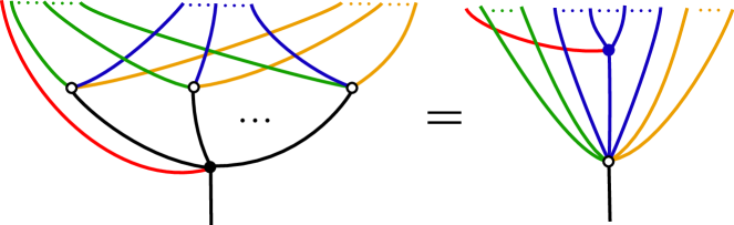
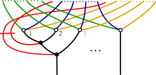
of degree , such that , and satisfying the -functor relations (a visual representation of which is given in Figure 1):
| (29) |
The sign is the Koszul sign obtained by commuting (equipped with degree ) to the front of the expression (where each is equipped with its reduced degree ). We henceforth adopt the convention, in expressions involving multifunctors, that is the Koszul sign associated to re-ordering the inputs in the expression so that they appear in the order (still equipping the with their reduced degrees).
If is strictly unital (with units denoted ), we say that is strictly unital in the th entry if
Lemma 37.
An -functor induces a functor
(the tensor product on the left is defined by considering each as a category with trivial differential – in particular the composition involves the Koszul sign rule). The action on objects is obvious, and on morphisms it sends
If is strictly unital in all entries, then this functor is unital.
Proof 5.2.
The components of define functors for each , which induce functors by taking cohomology. It now suffices to check that elements in (distinct) images of these functors supercommute, which is a consequence of the following -functor relation, written in the case to avoid notational clutter:
| (30) |
The unitality part of the claim is straightforward.
Example 5.3.
Let be categories, and their tensor product category. Then there is an -functor
and all other vanishing.
Definition 38.
Suppose that we have multifunctors for , and . We define the composition
It acts on objects in the obvious way, and on morphisms by analogy with composition of functors:
| (31) |
The check that the maps satisfy the multifunctor equations is straightforward. It is also easy to check that composition is ‘associative’ in the obvious sense.
Lemma 39.
Let and be -linear categories, and the category of bimodules. There is an tri-functor
defined on the level of objects by
and on the level of morphisms as follows:
-
•
For , we define
to be the morphism which sends
-
•
For , we define
to be the morphism which sends
is strictly unital in its first entry.
Lemma 40.
Let and be functors. Then there is a functor
It is given on the level of objects by defining to be the bimodule with
| (32) |
It is given on the level of morphisms by mapping the bimodule pre-homomorphism to the bimodule pre-homomorphism , given by the same formula (32), but with ‘’ replaced by ‘’.
Lemma 41.
Let and be functors, and denote by
the tri-functor introduced in Lemma 39, for . Then we have an equality
of tri-functors .
Lemma 42.
Suppose that are categories, is the category corresponding to a category , and is an -functor. Then there is an induced chain map
| (33) |
To clarify the notation: the first term is obtained by taking terms, and combining them with applications of into a single term. The overbraces signify that we sum over all cyclic permutations of the inputs such that lands underneath the overbrace labelled . As usual, is the Koszul sign associated to re-ordering the inputs : this includes the Koszul signs associated with the cyclic re-ordering associated with the overbrace notation, exactly as in Section 3.4. The other contribution to the overall sign is
Lemma 43.
5.3 The Mukai pairing for bimodules
Definition 45.
If is an object of a cohomologically unital category , then the cohomological unit defines a Hochschild cycle; we call the corresponding class in Hochschild homology the Chern character of , and denote it .
Lemma 46.
If and are quasi-isomorphic objects of , then .
Proof 5.4.
Let and be inverse isomorphisms. Then
so
so the classes and are cohomologous.
Definition 47.
Definition 47 is compatible with the corresponding notion in the world (25). To see how, we must first say how to turn a bimodule into an bimodule:
Definition 48.
Let and be -linear categories, and a bimodule. We define an bimodule with ,
If is the diagonal bimodule, then is tautologically isomorphic to the diagonal bimodule (as defined in [Sei08a, Equation (2.20)]).
Lemma 49.
If and are categories, and is a bimodule, then the diagram
commutes. Here, the top arrow is the tautological isomorphism , tensored with the isomorphism induced by the isomorphism of Remark 3.2.
Proof 5.5.
The diagram commutes on the level of cochain complexes: this follows by comparing Shklyarov’s formula (28) with our own definition.
Definition 50.
Proposition 51.
Let and be proper categories which are Morita equivalent. Then the isomorphism of Lemma 31 respects Mukai pairings.
Proof 5.6.
By Theorem 24, it suffices to consider the case that the Morita equivalence is induced by a functor which is cohomologically full and faithful and whose image split-generates. We will argue that
The first equality follows by combining Lemma 41 with Lemma 43. To prove the second we observe that, because is cohomologically full and faithful, is quasi-isomorphic to in (cf. the proof of Lemma 74). Hence, by Lemma 46, their Chern characters coincide, so the second equality is obvious from Definition 47. Composing with the Feigin–Losev–Shoikhet trace completes the proof.
Proposition 52.
Proof 5.7.
Proposition 53.
If is an category with finite-dimensional -spaces (i.e., finite-dimensional on the cochain level, not just on the cohomology level), then the Mukai pairing is induced by the following chain-level map: if and , then
| (35) | ||||
To clarify (35): if the expression is not composable in , we set the summand to be . ‘’ represents an element in the corresponding -space of .
Proof 5.8.
Example 5.9.
We recall that an category is called smooth (or homologically smooth) if the diagonal bimodule is perfect, i.e., split-generated by tensor products of Yoneda modules (see [KS08]). An category which is proper and smooth is called saturated.
Proposition 54.
If is saturated, then the Mukai pairing is non-degenerate.
5.4 Higher residue pairing on categories
We recall the definition of the higher residue pairing given in [Shk16]. If and are categories, then there is a Künneth map of cochain complexes, extending (24):
| (36) |
and similarly for the other versions of cyclic homology (see [Shk16, Proposition 2.5]). This map induces an isomorphism on periodic cyclic homology, but need not induce an isomorphism on negative cyclic homology.
As before, a bimodule induces a functor ; composing this with the Künneth map (36) yields a map
| (37) |
Because the inclusion induces a quasi-isomorphism of Hochschild chain complexes, it also induces a quasi-isomorphism of cyclic homology complexes, by Corollary 18. We therefore obtain a quasi-isomorphism . We know that (c.f. [Lod92, (2.1.12)]), so we obtain an isomorphism on the level of cohomology:
| (38) |
the ‘cyclic Feigin–Losev–Shoikhet trace’ (and similarly for periodic cyclic homology, where the map is to , and positive cyclic homology, where the map is to ).
The -linear extension of the map defined in Lemma 35 defines a chain map
The same argument as given in the proof of Lemma 35 shows that the induced map on the level of cohomology coincides with the map
Definition 55.
If is a proper category, we define the higher residue pairing, which is the pairing
The pairing is sesquilinear. We obtain similar pairings on and .
Because the Künneth quasi-isomorphism for negative cyclic homology (36) extends that for Hochschild homology (24), and because the cyclic Feigin–Losev–Shoikhet trace (38) extends the non-cyclic version (27), the higher residue pairing extends the Mukai pairing, in the sense that
where on the left-hand side, is the map setting , and on the right-hand side, is the map induced on Hochschild complexes.
5.5 Higher residue pairing for bimodules
Definition 56.
Let be an tri-functor, where . We define a -linear map
as a sum of three maps: . For , , , we define
| (39) |
where is Koszul sign associated to re-ordering the inputs as before (ignoring ), and is the Koszul sign associated to commuting (equipped with sign ) to the front of the expression, where all have degree , all have their reduced degrees, and has degree .
We define
| (40) |
We define
| (41) |
Lemma 57.
Proof 5.11.
Definition 58.
As in Definition 45, any object of an category has an associated ‘cyclic Chern character’ (similarly for periodic and positive versions). Quasi-isomorphic objects have the same cyclic Chern character. If is strictly unital, the Chern character has a particularly simple cochain-level representative. Namely, in the presence of strict units, we can define the Connes differential (and all other operations we have considered so far) using the strict units in place of . This gives the unital cyclic complex . In the unital cyclic complex, is represented on the cochain level by the length- cycle .
We do not give a proof of the assertions made in Definition 58, but they are standard: in fact, one can show that depends only on the class of (cf. [Sei, Lemma 8.4]).
Definition 59.
Lemma 60.
Definition 59 is compatible with the corresponding definition in the world, i.e., the following diagram commutes:
Here, the horizontal arrows are the tautological identifications (or the isomorphism induced by the the isomorphism of Remark 3.2, in the case of ). The left vertical map is the map (37), and the right vertical map is the map introduced in Definition 59.
Proof 5.12.
The diagram commutes on the level of cochain complexes.
Definition 61.
Let be a proper category. We define the higher residue pairing
| (42) |
where is the diagonal bimodule, is as in Definition 59, denotes the cyclic Feigin–Losev–Shoikhet trace (which we can apply because is proper), and is the image of under the isomorphism of Remark 3.5. The higher residue pairing is -sesquilinear.
Proposition 62 (Morita invariance of higher residue pairing).
Let and be proper categories, which are Morita equivalent. Then the isomorphism of Corollary 33 respects higher residue pairings.
Proof 5.13.
The proof follows that of Proposition 51 closely.
Proposition 63.
Proposition 64.
If is an category with finite-dimensional -spaces (i.e., finite-dimensional on the cochain level, not just on the cohomology level), then the higher residue pairing is induced by a chain-level map, given by extending the formula (35) -sesquilinearly.
Proof 5.15.
Observe that is strictly unital, so we have the explicit representing cycle for , as explained in Definition 58. We now observe that , so on the chain level we have
Now observe that never outputs a term of length (see Definition 56), so on the chain level. The proof now follows from that of Proposition 53.
5.6 The higher residue pairing is covariantly constant
Definition 65.
Let be a -linear category with finite-dimensional -spaces, together with a choice of basis for each -space (which we recall is necessary to make sense of expressions like ‘’). For each derivation , we define a -sesquilinear map
as a sum of three terms: . For and , we define
| (43) |
| (44) |
| (45) |
Lemma 66.
We have
as -sesquilinear maps from .
Corollary 67.
Let be a proper -linear category. Then the higher residue pairing is covariantly constant with respect to the Getzler–Gauss–Manin connection: i.e., for any , we have
as -sesquilinear maps from .
Proof 5.16.
By the homological perturbation lemma, any category is quasi-isomorphic to a minimal category (i.e., one with ). We have , and the isomorphism respects connections (Theorem 20) and higher residue pairings (Proposition 62), so it suffices to prove the result for . Because is proper, will have finite-dimensional -spaces, so its higher residue pairing is covariantly constant by Lemma 66.
5.7 Symmetry
Let be a bimodule. We recall the definition of the shift, , which is a bimodule with (see [Sei08a, Equation (2.10)]).
Lemma 68.
Let be a proper bimodule. Then
Proof 5.17.
We may assume that and are categories, and a proper bimodule. We recall that corresponds to a functor , and that Shklyarov [Shk12] defines to be the map induced by this functor on Hochschild homology, composed with the Künneth isomorphism. It is clear that corresponds to the composition of functors , where is the shift functor. It now suffices to check that , where is the map induced by the functor . Because the inclusion is a quasi-equivalence, it suffices by Lemma 35 to prove that on . This is clear from the definition of the supertrace.
We also recall the linear dual bimodule, , which is a bimodule with (see, e.g., [Sei17, Equation (2.11)]).
Lemma 69.
Let be a proper bimodule. Then
Proof 5.18.
Once again, we may assume that , and are , and regard as a functor. The proof combines four pieces. First, let denote the following composition of functors:
where the first functor sends and ‘’ denotes the functor that dualizes cochain complexes. One easily verifies that this is compatible with the definition, in the sense that .
Second, for any functor , one easily checks that (we apply this to ).
Third, one checks that the following diagram commutes:
where the horizontal arrows are the Künneth maps [Shk12, Section 2.4], the left vertical arrow combines the isomorphism of [Shk12, Equation (4.8)] (and similarly for ) with the Koszul isomorphism , and the right vertical arrow is induced by the isomorphism composed with the map induced by the isomorphism of categories, .
Fourth, one checks that . As in the proof of Lemma 68, it suffices to prove that ; and this reduces to the obvious fact that the trace of the dual of a matrix coincides with the trace of the original matrix. Combining the four pieces gives the result.
We recall that an -dimensional weak proper Calabi–Yau structure on an category is a quasi-isomorphism (see [Sei08b, Section 12j], as well as [Tra08] and [She16, Section A.5], where it is called an ‘-inner product’).
Lemma 70.
If admits an -dimensional weak proper Calabi–Yau structure, then the Mukai pairing on satisfies:
Similarly for the higher residue pairing.
Proof 5.19.
5.8 Hodge-to-de Rham degeneration
Definition 71.
Suppose that is saturated. We say that satisfies the degeneration hypothesis if the spectral sequence (13) induced by the Hodge filtration on degenerates at the page.
A conjecture of Kontsevich and Soibelman [KS08, Conjecture 9.1.2] asserts that all saturated categories satisfy the degeneration hypothesis. It has been proved by Kaledin [Kal17] (see also [Mat]), in the case that is -graded.
Proof 5.20.
Any category is quasi-equivalent to a category, via the Yoneda embedding; so let us assume without loss of generality that is . Then is finite-dimensional and the Mukai pairing is non-degenerate, by [Shk12, Theorem 1.4]; it follows that the polarization given by the higher residue pairing is non-degenerate.
As an immediate consequence, the spectral sequence (13) induced by the Hodge filtration on any of is automatically bounded (by the degree bound on ) and regular (by finite-dimensionality); because the Hodge filtration is complete and exhaustive, the complete convergence theorem [Wei94, Theorem 5.5.10] implies that the spectral sequence converges to its cohomology. Hence, has finite rank.
Appendix A Morita equivalence
In this Appendix we provide proofs of some well-known results relating to Morita equivalence of categories.
Lemma 73.
Let be a homomorphism of bimodules. Let and be subsets which split-generate and respectively. If the map
| (46) |
is a quasi-isomorphism for all , then is a quasi-isomorphism.
Proof A.1.
Denote by the set of objects such that (46) is a quasi-isomorphism for all . This set contains by hypothesis, and it is straightforward to show that it is closed under forming cones and direct summands; therefore it is all of because split-generates. Now repeat the argument for the set of objects such that (46) is a quasi-isomorphism for all .
Lemma 74 (=Lemma 23).
If is a cohomologically full and faithful functor, and is split-generated by the image of , then and define a Morita equivalence between and .
Proof A.2.
Tensor products of bimodules respect pullbacks in the following sense: If are functors for , then there is a morphism of bimodules
| (47) |
It is given by the formula
(no higher maps). If is the identity functor, it is clear from the formula that (47) is the identity. It follows immediately that . Now there is a natural morphism , given by contracting all terms with . This morphism is clearly a quasi-isomorphism when is cohomologically full and faithful. Therefore, as required.
It remains to prove that . From (47), we obtain a morphism of bimodules
| (48) |
So it remains to prove that this morphism is a quasi-isomorphism of bimodules. The linear term of (48) is the map
| (49) |
given by the formula
| (50) |
We now prove that (49) is a quasi-isomorphism in the special case that and . To do this, we observe that the following diagram commutes up to homotopy:
| (51) |
The left vertical map sends
(compare [Ganb, Equation (2.240)]). The bottom horizontal map is precisely the map (49). The diagram commutes up to the homotopy given by
using the functor equations for . Furthermore, the top horizontal arrow is a quasi-isomorphism (it is the first term in the quasi-isomorphism ); the right vertical arrow is a quasi-isomorphism (because is cohomologically full and faithful); the left vertical arrow is a quasi-isomorphism, by a comparison argument for the spectral sequences induced by the obvious length filtrations, again using the fact that is cohomologically full and faithful. It follows that the bottom map is a quasi-isomorphism. So (49) is a quasi-isomorphism when and are in the image of .
Theorem 75.
If and are Morita equivalent, then and are quasi-equivalent.
Proof A.3.
This is a consequence of [Sta18, Proposition 13.34.6], which is due to [TT90] and [Nee92] (see also [Kel06, Theorem 3.4]). Namely, we consider the category of right -modules: its cohomological category is a triangulated category, which admits arbitrary coproducts and is compactly generated by the Yoneda modules. We call an object of compact if the corresponding object of the triangulated category is compact in the usual sense. Then, the subcategory of compact objects of is precisely the triangulated split-closure of the image of the Yoneda embedding, by the above-mentioned theorem. We refer to it as : it is quasi-equivalent to by the uniqueness of triangulated split-closures [Sei08b, Lemma 4.7].
Now suppose and are Morita equivalent. Then we have a quasi-equivalence , given by tensoring with the Morita bimodule. As a consequence, the respective subcategories of compact objects, and , are quasi-equivalent: hence and are quasi-equivalent.
Appendix B Functoriality of the Getzler–Gauss–Manin connection
The aim of this appendix is to prove Theorem 20.
Lemma 76.
Let be an functor. Define by
| (52) |
and
| (53) |
Define . Then
for all . In particular, on the level of cohomology,
Proof B.1.
By the functor equation,
| (54) |
for all . Pre-compose this relation with the map , defined by
One obtains
| (55) |
where
| (56) |
| (57) |
| (58) |
| (59) |
| (60) |
| (61) |
By the relations , we find that
| (62) |
where
| (63) |
| (64) |
| (65) |
| (66) |
By differentiating the functor equation, we find that
| (67) |
where
| (68) |
| (69) |
We now compute that
| (70) |
all other terms cancel by the functor equations (note: here, ‘’ simply denotes composition of functions, not Gerstenhaber product). We similarly compute that
| (71) |
(we must apply the functor equation to obtain the terms and ).
Theorem 77.
Proof B.2.
Define by
Let be defined by . We will prove that
| (72) |
from which the result follows.
It suffices to prove (72) for , by -linearity. We separate it into powers of : it is clear that the term vanishes for all except . The component of (72) says
| (73) |
which holds by Lemma 76. The component of (72) says
| (74) |
First, by differentiating the functor equation, we obtain the relation
| (75) |
where
| (76) |
| (77) |
| (78) |
| (79) |
Now, we compute each pair of terms in (74) separately. We compute
| (80) |
where
| (81) |
| (82) |
Next, we compute
| (83) |
where
| (84) |
| (85) |
(all other terms cancel by the functor equations). Next, we compute
| (86) |
where
| (87) |
(all other terms cancel by the functor equations). Next, we compute
| (88) |
and
| (89) |
Next, we compute
| (90) |
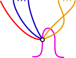
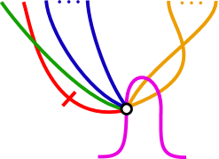
Appendix C Graphical sign convention
In this appendix we explain a convenient notation for checking formulae in algebra, including the signs and gradings.
C.1 The idea
The idea is to represent compositions of multilinear operations by a diagram as in Figure 1, which we call a sign diagram. The inputs will always be at the top of the diagram, and the outputs at the bottom. Strands in the diagram are allowed to cross, but no three strands should meet at a point.
Each strand in the diagram is oriented (from input to output), and carries a degree. By convention, strands which correspond to morphisms in our category will carry their reduced degree, . Also by convention, the sum of the degrees of the edges coming into each vertex must be equal to the sum of the degrees going out. This convention forces us to add a red strand coming into each vertex, carrying the degree of the corresponding operation (we omit it when the degree is zero). This is the case, for example, for the operations , which have degree with respect to the reduced degree.
To any sign diagram , we associate a sign , as follows: to each crossing of strands, we associate the product of the degrees of those strands (the Koszul sign associated to commuting the corresponding two variables). Then is the sum of these signs, over all crossings in the diagram.
Definition 78.
We say two sign diagrams are isotopic if they are related by a sequence of moves of the following two types: moving a strand over a crossing; and moving a strand over a vertex.
Lemma 79.
If sign diagrams and are isotopic, then .
Proof C.1.
It is trivial that moving a strand over a crossing does not change the sign. When one moves a strand over a vertex, the sign does not change because of the assumption that the sum of the degrees going into the vertex is equal to the sum of the degrees going out.
If we assign multilinear operations to the vertices in our sign diagram, then the sign diagram gives us a prescription for composing the operations: by convention, this composition gets multiplied by the sign associated to the sign diagram. By Lemma 79, isotopic sign diagrams give the same sign, and they also obviously give the same composition of operations: so they represent the same composed operation.
C.2 Sign diagrams for operations in this paper
In this section we give the sign diagrams associated to some of the more complicated formulae in this paper.
References
- [Amo16] Lino Amorim, Tensor product of filtered -algebras, J. Pure Appl. Algebra 220 (2016), no. 12, 3984–4016. MR 3517566
- [AT] Lino Amorim and Junwu Tu, Categorical primitive forms of Calabi–Yau -categories with semi-simple cohomology, Preprint, available at arXiv:1909.05319.
- [Bar01] Serguei Barannikov, Quantum periods. I. Semi-infinite variations of Hodge structures, Internat. Math. Res. Notices (2001), no. 23, 1243–1264. MR 1866443
- [Bar02] , Non-commutative periods and mirror symmetry in higher dimensions, Comm. Math. Phys. 228 (2002), no. 2, 281–325. MR 1911737
- [Bla16] Anthony Blanc, Topological K-theory of complex noncommutative spaces, Compos. Math. 152 (2016), no. 3, 489–555. MR 3477639
- [CdlOGP91] Philip Candelas, Xenia de la Ossa, Paul Green, and Linda Parkes, A pair of Calabi-Yau manifolds as an exactly soluble superconformal theory, Nuclear Physics B 359 (1991), no. 1, 21–74.
- [CIT09] Tom Coates, Hiroshi Iritani, and Hsian-Hua Tseng, Wall-crossings in toric Gromov-Witten theory I: crepant examples, Geometry & Topology 13 (2009), no. 5, 2675–2744.
- [CK99] David Cox and Sheldon Katz, Mirror Symmetry and Algebraic Geometry, American Mathematical Society, 1999.
- [Cos07] Kevin Costello, Topological conformal field theories and Calabi-Yau categories, Advances in Mathematics 210 (2007), no. 1, 165–214.
- [Cos09] , The partition function of a topological field theory, J. Topol. 2 (2009), no. 4, 779–822. MR 2574744
- [Gana] Sheel Ganatra, Cyclic homology, -equivariant Floer cohomology, and Calabi-Yau structures, Preprint, available from https://sheelganatra.com/circle_action/circle_action.pdf.
- [Ganb] , Symplectic Cohomology and Duality for the Wrapped Fukaya Category, Preprint, available at arXiv:1304.7312.
- [Ger63] Murray Gerstenhaber, The cohomology structure of an associative ring, Ann. of Math. (2) 78 (1963), 267–288. MR 0161898
- [Get93] Ezra Getzler, Cartan homotopy formulas and the Gauss-Manin connection in cyclic homology, Israel Math. Conf. Proc. 7 (1993), 1–12.
- [Giv95] Alexander Givental, Homological geometry and mirror symmetry, Proceedings of the International Congress of Mathematicians, Vol. 1, 2 (Zürich, 1994), Birkhäuser, Basel, 1995, pp. 472–480. MR 1403947
- [Giv96] , Equivariant Gromov-Witten invariants, Int. Math. Res. Not. 1996 (1996), no. 13, 613–663.
- [GPSa] Sheel Ganatra, Timothy Perutz, and Nick Sheridan, The cyclic open–closed map and noncommutative Hodge structures, In progress.
- [GPSb] , Mirror symmetry: from categories to curve counts, Preprint, available at arXiv:1510.03839.
- [Gro11] Mark Gross, Tropical geometry and mirror symmetry, CBMS Regional Conference Series in Mathematics, 114. American Mathematical Society, Providence RI, 2011.
- [Kal07] Dmitry Kaledin, Some remarks on formality in families, Mosc. Math. J. 7 (2007), no. 766, 643–652.
- [Kal17] , Spectral sequences for cyclic homology, Algebra, geometry, and physics in the 21st century, Progr. Math., vol. 324, Birkhäuser/Springer, Cham, 2017, pp. 99–129. MR 3702384
- [Kel06] Bernhard Keller, On differential graded categories, International Congress of Mathematicians. Vol. II, Eur. Math. Soc., Zürich, 2006, pp. 151–190.
- [KKP08] Ludmil Katzarkov, Maxim Kontsevich, and Tony Pantev, Hodge theoretic aspects of mirror symmetry, From Hodge theory to integrability and TQFT tt*-geometry, Proc. Sympos. Pure Math. 78 (2008), 87–174.
- [Kon95] Maxim Kontsevich, Homological algebra of mirror symmetry, Proceedings of the International Congress of Mathematicians, Vol. 1, 2 (Zürich, 1994), Birkhäuser, Basel, 1995, pp. 120–139. MR 1403918
- [KS08] Maxim Kontsevich and Yan Soibelman, Notes on A-infinity algebras, A-infinity categories and non-commutative geometry. I, Homological Mirror Symmetry: New Developments and Perspectives, Lecture Notes in Physics, vol. 757, Springer, 2008, pp. 153–219.
- [LLY97] Bong Lian, Kefeng Liu, and Shing-Tung Yau, Mirror Principle I, Asian Journal of Mathematics 1 (1997), no. 4, 729–763.
- [Lod92] Jean-Louis Loday, Cyclic homology, Grundlehren der Mathematischen Wissenschaften [Fundamental Principles of Mathematical Sciences], vol. 301, Springer-Verlag, Berlin, 1992, Appendix E by María O. Ronco. MR 1217970
- [Lun10] Valery Lunts, Formality of DG algebras (after Kaledin), J. Algebra 323 (2010), no. 4, 878–898. MR 2578584
- [Lyu15] Volodymyr Lyubashenko, -morphisms with several entries, Theory Appl. Categ. 30 (2015), Paper No. 45, 1501–1551. MR 3421458
- [Mat] Akhil Mathew, Kaledin’s degeneration theorem and topological Hochschild homology, Preprint, available at arXiv:1710.09045.
- [Mor93] David Morrison, Mirror symmetry and rational curves on quintic threefolds: A guide for mathematicians, Journal of the American Mathematical Society 6 (1993), no. 1, 223–247.
- [Nee92] Amnon Neemann, The connection between the K-theory localization theorem of Thomason, Trobaugh and Yao and the smashing subcategories of Bousfield and Ravenel, Annales Scientifiques de L’E.N.S. (4) 25 (1992), no. 5, 547–566.
- [Orl04] Dmitri Orlov, Triangulated categories of singularities and D-branes in Landau–Ginzburg models, Proc. Steklov Inst. Math. 246 (2004), 227–248.
- [PSa] Timothy Perutz and Nick Sheridan, Automatic split-generation for the Fukaya category, Preprint, available at arXiv:1510.03848.
- [PSb] , Foundations of the relative Fukaya category, In preparation.
- [Sai83] Kyoji Saito, Period mapping associated to a primitive form, Publ. Res. Inst. Math. Sci. 19 (1983), no. 3, 1231–1264. MR 723468
- [Sei] Paul Seidel, Lectures on Categorical Dynamics and Symplectic Topology, Available from http://www-math.mit.edu/~seidel/.
- [Sei08a] , subalgebras and natural transformations, Homology, Homotopy Appl. 10 (2008), no. 2, 83–114.
- [Sei08b] , Fukaya categories and Picard-Lefschetz theory, Zurich Lectures in Advanced Mathematics, European Mathematical Society (EMS), Zürich, 2008. MR 2441780
- [Sei17] , Fukaya -structures associated to Lefschetz fibrations. II, Algebra, geometry, and physics in the 21st century, Progr. Math., vol. 324, Birkhäuser/Springer, Cham, 2017, pp. 295–364. MR 3727564
- [She] Nick Sheridan, Versality of the relative Fukaya category, Preprint, available at arXiv:1709.07874.
- [She15] , Homological mirror symmetry for Calabi-Yau hypersurfaces in projective space, Invent. Math. 199 (2015), no. 1, 1–186.
- [She16] , On the Fukaya category of a Fano hypersurface in projective space, Publ. Math. Inst. Hautes Études Sci. 124 (2016), 165–317. MR 3578916
- [Shk12] Dmytro Shklyarov, Hirzebruch–Riemann–Roch-type formula for DG algebras, Proc. Lond. Math. Soc. 106 (2012), no. 1, 1–32.
- [Shk16] , Matrix factorizations and higher residue pairings, Adv. Math. 292 (2016), 181–209. MR 3464022
- [Sim97] Carlos Simpson, The Hodge filtration on nonabelian cohomology, Algebraic geometry—Santa Cruz 1995, Proc. Sympos. Pure Math., vol. 62, Amer. Math. Soc., Providence, RI, 1997, pp. 217–281. MR 1492538
- [Sta18] The Stacks Project Authors, Stacks Project, https://stacks.math.columbia.edu, 2018.
- [Tra08] Thomas Tradler, Infinity-inner-products on A-infinity-algebras, J. Homotopy Relat. Struct. 3 (2008), no. 1, 245–271.
- [TT90] Robert Thomason and Thomas Trobaugh, Higher algebraic -theory of schemes and of derived categories, The Grothendieck Festschrift, Vol. III, Progr. Math., vol. 88, Birkhäuser Boston, Boston, MA, 1990, pp. 247–435. MR 1106918
- [Tu] Junwu Tu, Categorical Saito theory, II: Landau-Ginzburg orbifolds, Preprint, available at arXiv:1910.00037.
- [Voi07] Claire Voisin, Hodge theory and complex algebraic geometry. II, english ed., Cambridge Studies in Advanced Mathematics, vol. 77, Cambridge University Press, Cambridge, 2007, Translated from the French by Leila Schneps. MR 2449178
- [Wei94] Charles Weibel, An introduction to homological algebra, Cambridge University Press, Cambridge Studies in Advanced Mathematics, 38, 1994.