TraMoS IV: Discarding the Quick Orbital Decay Hypothesis for OGLE-TR-113b

Abstract

In the context of the TraMoS project we present nine new transit observations of the exoplanet OGLE-TR-113b observed with the Gemini South, Magellan Baade, Danish-1.54m and SOAR telescopes. We perform a homogeneous analysis of these new transits together with ten literature transits to probe into the potential detection of an orbital decay for this planet reported by Adams et al. (2010). Our new observations extend the transit monitoring baseline for this system by 6 years, to a total of more than 13 years. With our timing analysis we obtained a $\dot{P}=-1.0\pm 6.0$ ms yr^-1, which rejects previous hints of a larger orbital decay for OGLE-TR-113b. With our updated value of $\dot{P}$ we can discard tidal quality factors of $Q_{\star}<10^{5}$ for its host star. Additionally, we calculate a 1$\sigma$ dispersion of the Transit Timing Variations (TTVs) of 42 seconds over the 13 years baseline, which discards additional planets in the system more massive than $0.5-3.0~{}M_{\oplus}$ in 1:2, 5:3, 2:1 and 3:1 Mean Motion Resonances with OGLE-TR-113b. Finally, with the joint analysis of the 19 light curves we update transit parameters, such as the relative semi-major axis $a/R_{s}=6.44^{+0.04}_{-0.05}$, the planet-to-star radius ratio $R_{p}/R_{s}=0.14436^{+0.00096}_{-0.00088}$, and constrains its orbital inclination to $i=89.27^{+0.51}_{-0.68}$ degrees.

1 Introduction

OGLE-TR-113b was one of the first discovered transiting exoplanets, reported by Udalski et al. (2002) as a planet candidate orbiting a V = 16.1 K-dwarf star, and later confirmed by Bouchy et al. (2004) and Konacki et al. (2004) via radial velocity follow-up campaigns. With a mass of 1.23 $M_{\rm Jup}$ and a radius of 1.09 $R_{\rm Jup}$ (Southworth, 2012), OGLE-TR-113b is a hot Jupiter orbiting its host star once every 1.43 days. Due to the proximity to its host star, OGLE-TR-113b is potentially an interesting target for orbital decay by tidal dissipation studies (see e.g. Sasselov, 2003; Pätzold et al., 2004; Carone & Pätzold, 2007; Levrard et al., 2009; Matsumura et al., 2010; Penev & Sasselov, 2011; Penev et al., 2012), in which it is predicted that the orbital separation between the star and the planet will continue to shrink – in spite of orbital circularization – as long as the orbital motion of the planet is faster than the stellar rotation rate. In those cases, the planet’s orbital decay will continue until the planet reaches the stellar Roche radius limit of the system and falls into the star (see e.g. Levrard et al., 2009).

Although the orbital decay of exoplanets is a topic that has received increasing attention over the past decade, estimations of the expected timescales of this effect remain largely unconstrained because of the currently limited understanding and measurements of tidal dissipation mechanisms in both planets and stars. Because of this lack of understanding, tidal quality factors, which are a measure of the star or planet’s distorstion due to tidal effects and drive the efficiency of the orbital time decay, are generally allowed to adopt a wide range of values, between $Q_{\star}=10^{4}$ – $10^{10}$ (see e.g. Pätzold et al., 2004; Matsumura et al., 2010).

Directly measuring the orbital decay of a close-in, short period, exoplanet would enable the first empirical test to current tidal stability and dynamical models of these objects. A way to detect that orbital decay is via long-term monitoring campaigns of transiting exoplanets in search for small and steady transit timing variations (TTVs; see e.g. Miralda-Escudé, 2002; Holman & Murray, 2005; Agol et al., 2005), which would show the transits occurring systematically closer in time over timescales of several years.

Adams et al. (2010), hereafter A10, reported the tentative detection of an orbital period decay of $\dot{P}=-60\pm 15$ ms yr^-1 for OGLE-TR-113b, but the authors acknowledged that more observations were needed to confirm their claim. That period decay rate could be reproduced by a relatively small tidal quality factor for the star of $Q_{\star}\sim 10^{3}-10^{4}$ (Birkby et al., 2014), which is close to the theoretical lowest estimate for this parameter. Additionally, Penev et al. (2012) concluded that the population of currently known planets is inconsistent at the 99$\%$ level with $Q_{\star}>10^{7}$.

OGLE-TR-113b is one of the targets we have been monitoring in our Transit Monitoring in the South (TraMoS) project, which includes observations from the 1-m telescope at CTIO, SOAR and Gemini South telescopes at Cerro Pachón Observatory (Hoyer et al., 2012). TraMoS, which has been underway since 2008, is dedidacted to searching for transit timing variations of known planets to unveil additional planets in those systems and, therefore, their architecture. Other planetary systems we have published as part of TraMoS are OGLE-TR-111b WASP-5b and WASP-4b (see Hoyer et al., 2011, 2012, 2013).

In this work we present eight new transit light curves of OGLE-TR-113b from TraMoS, observed with Gemini South, SOAR and Danish-1.54m telescopes, and a new transit light curve obtained with the same instrumental setup used by A10 on Magellan. We combine those new light curves with all available literature light curves to perform a new study of transit timing variations for this system. In Section 2 we describe the observations. Section 3 describes the data analysis and light curve fitting. Sections 4 and 5 describe the timing analysis and mass limits for unseen perturbers, and we present our conclusions in Section 6.

Epoch	Date Obs.	Instrument /	Filter	Average	Airmass range	# points
	(yyyymmdd)	Telescope		Cadence (s)
192	20060104	GMOS/Gemini-S	g’	75 / 330	2.34 - 1.18	120
946	20081219	GMOS/Gemini-S	g’	54	2.07 - 1.29	180
953	20081229	GMOS/Gemini-S	g’	54	1.67 - 1.21	206
969	20090121	GMOS/Gemini-S	g’	54	1.65 - 1.20	213
990	20090220	GMOS/Gemini-S	i’	44	1.19 - 1.31	284
992	20090223	GMOS/Gemini-S	i’	49	1.58 - 1.17	381
1471	20110110	MagIC-e2V/Magellan	i’	62	1.47 - 1.19	241
2530	20150306	DFOSC/Danish-1.54m	R	144	1.19 - 1.99	161
2585	20150624	SOI/SOAR	I	57	1.18 - 1.92	239

Table 1: Description of each of the nine new transit observations presented in this work.

2 Observations and Photometry

We observed OGLE-TR-113b during nine transit epochs between 2006 and 2015. The first six transits were observed with the Gemini Multi-Object Spectrograph (GMOS-S) instrument on the 8.1m Gemini South Telescope (programs ID: GS-2005B-Q-9, GS-2008B-Q-11, GS-2009A-Q-16 and GS-2010A-Q-36). GMOS-S in imaging mode has a pixel scale of 0.073 $arcsec/pixel$ and a Field-of-View (FoV) of 330$\times$300 $arcsec^{2}$. However, for these observations we used a Region of Interest (RoI) which includes only the central 1024 rows, reducing the readout time of the detector to only $\sim$47 seconds. The FoV of the RoI is 75 $\times$ 168 $arcsec^{2}$, which given the relatively crowded field of OGLE-TR-113b, contains enough comparison stars to perform precise differential photometry. In addition, the high resolution of the pixels minimizes blends.

The transit on 2006-01-04 ($E=192$, where we use as $E=0$ the transit of 2005-04-04 from Gillon et al. (2006) described below), was observed alternating between the GMOS g’(G0325) and GMOS i’ (G0327) filters with exposures of 30 seconds each. Unfortunately, the GMOS i’ images were saturated and are not included in this work. The next three transits were observed in the GMOS g’(G0325) filter and the last two epochs were observed with the GMOS i’ (G0327) filter. Each observation lasted between 3.1 to 5.4 hours, and included the full transit and out of eclipse baseline. The dates and other specific details of each transit observation are summarized in Table 1.

The transit of 2011-01-10 was observed with the MagIC-e2v camera on the 6.5m Baade Telescope at Las Campanas Observatory, and with the same setup described in A10. MagIC-e2v has a FoV of 38$\times$38 $arcsec^{2}$, with a resolution of 0.037 $arcsec/pixel$. The frame transfer mode of MagIC-e2v provides a readout of 0.003 seconds per frame, which highly surpasses the readout of conventional cameras, such as GMOS-S. The observations were done in unbinned mode, with a Sloan i’ filter, and an exposure time of 30 seconds per frame. The observations lasted 4.1 hours, and include the full transit and out of transit baseline.

The 2015-03-06 transit was observed using the DFOSC (Danish Faint Object Spectrograph and Camera) camera on the 1.54m Danish Telescope at ESO La Silla Observatory. DFOSC has a field of view of 13.7’$\times$13.7’ at a plate scale of 0.396 $arcsec/pixel$. We used unbinned mode, with the $Bessel~{}R$ filter and an exposure time of 100 seconds.

The last transit, 2015-06-24, was obtained with SOI (SOAR Optical Imager) on the 4.1m Southern Astrophysical Research (SOAR) Telescope at Cerro Pachón Observatory. SOI is a mini-mosaic of two E2V 2k$\times$4k CCDs with a FoV of 5.26’$\times$5.26’ and a pixel scale of 0.077 $arcsec/pixel$. We used a $Bessel~{}I$ filter and an exposure time of 45 seconds per frame in the 2x2 binned mode. At the end of the night the sky was covered by clouds which prevented observations of the egress and after-the-transit baseline.

To reduce the data, in the case of GMOS-S we used the processed images delivered by the Gemini telescope reduction pipeline. In the case of the MagIC-e2v, DFOSC and SOI data, we bias-corrected and flatfielded the images using standard IRAF routines.

The reduced images were ran through a custom, python-based pipeline developed for TraMoS. This pipeline performs aperture photometry of the target and a set of reference stars and combines them to create differential light curves, free of most Earth atmospheric effects. The aperture radius, sky annulus, and reference stars are determined iteratively by the pipeline, as those that produce the smallest dispersion of the out-of-transit light curves. In some datasets, where the seeing variations during the night are large, the pipeline allows for different values of the aperture and sky annulus throughout the night. The light curves of each of the nine new transits, which still contain some systematics effects that need to be modelled (see Section 3), are shown in Figure 1 along with the literature light curves described below.

2.1 Literature Light Curves

In our analysis we also included ten literature light curves: two light curves in R band collected on April 4 and 14 2005 UT (Gillon et al., 2006), a V band light curve collected on April 11 2005 UT (Pietrukowicz et al., 2010; Diaz et al., 2007), a light curve in K band observed on March 18 2006 UT (Snellen & Covino, 2007), and six light curves observed between January 30 2007 UT and May 10 2009 UT reported by A10. We used the compilation of all these light curves by A10.

3 Light Curve Modelling

We modelled our nine new transit light curves simultaneously with the literature light curves using the Transit Analysis Package (TAP v2.104, Gazak et al., 2012) Like in A10, we did not fit the Konacki et al. (2004) light curve, since it is the result of phase folded data from the OGLE survey over several transit epochs. Instead, we adopted their reported midtime of transit and used that value in parts of the TTV analysis described in Section 4.

We fit all the other light curves for the transits central time, $T_{c}$, the planet-to-star radius ratio ($R_{p}/R_{s}$), the orbital inclination ($i$), and a quadratic limb darkening law, with $u_{1}$ and $u_{2}$ as the linear and quadratic limb darkening coefficients. We also fit a linear function of the flux vs time ($Y_{int}$ and $Y_{slope}$) in order to remove systematics in the light curves, which are mostly produced by changes in the airmass during the observations. The amount of correlated and uncorrelated noise is also estimated in each light curve using the wavelet-based method proposed by Carter & Winn (2009), where the noise parameters, $\sigma_{w}$ (for the white noise) and $\sigma_{r}$ (for the correlated noise), are fitted from the light curves assuming the correlated noise follows a power spectral density varying as $1/f$.

We fixed the values of the orbital eccentricity, $e$, and longitude of periastron, $\omega$, to zero, and we adopted a fixed orbital period for the system of $P=1.43247425$  days from A10.

Having several transit epochs is advantageous to refine the values of some of the system’s parameters, such as $i$, $R_{p}/R_{s}$, and $a/R_{p}$. Therefore, we fit for those parameters using all the light curves, simultaneously, while letting $T_{c}$ vary individually for each transit. We found that we cannot produce reliable limb darkening fits on individual light curves. The fits also had problems distinguishing between very similar filters, e.g. between the Gemini $i^{\prime}$ and the MagIC $i^{\prime}$ filters, or the Gemini $g^{\prime}$ and $V$ filters. We got around this problem by fitting both limb darkening coefficients ($u_{1}$ and $u_{2}$) simultaneously for all the same filter light curves, i.e. $i^{\prime}$, $g^{\prime}$, $R$ and $K$, where we assumed that the limb darkening coefficients for similar filters were the same. Furthemore, based on Csizmadia et al. (2012), we do not fix the limb darkening coefficients to theoretical predictions but leave them as free parameters. The limb darkening coefficients obtained from the joint analysis of each filter are summarized in Table 2.

We ran 10 different MCMC chains of $10^{5}$ links each, discarding the first $10\%$ to avoid any bias introduced by initial values of the fitted parameters. Our fits yield refined values for $i$, $R_{p}/R_{s}$, and $a/R_{p}$, which are summarized in Table 2. In Table 3 we show the central time obtained for each transit. The raw transit light curves are shown in Figure 1, together with their best model fits. All the data are available online in tables including the times and normalized fluxes of each transit; Table 4 shows an excerpt of those tables.

We note in the $E=1471$ light curve a signature that can be attributed to star spot occultations of the planet during the transit. The transits $E=192$, $793$ and $992$ also show bumps in the light curves during transit but with very low amplitudes. Moreover, A10 reported that the bump in the $E=793$ light curve was produced by a rapid seeing variation. The large time span between these detections prevents us from carrying out a more detailed study of the rotational period of the star.

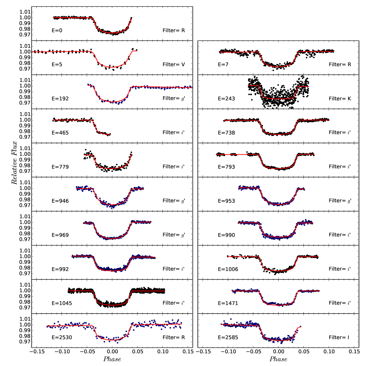
Figure 1: Transit light curves of OGLE-TR-113b. The nine transits presented in this work (blue points) are shown with the ten literature light curves (black points). Each transit is labeled with its respective epoch and filter. The transit models obtained with TAP are shown with the red solid lines.

Simultaneous Fitted Parameters
$a/R_{s}$	$6.44^{+0.04}_{-0.05}$
$(R_{p}/R_{s})$	$0.14436^{+0.00096}_{-0.00088}$
$i$ (deg)	$89.27^{+0.51}_{-0.68}$
Limb Darkening	$u_{1}$	$u_{2}$
R	$0.67^{+0.15}_{-0.18}$	$-0.03^{+0.29}_{-0.25}$
$g$’, V	$0.733^{+0.094}_{-0.089}$	$0.14^{+0.14}_{-0.15}$
K	$0.20^{+0.25}_{-0.15}$	$0.09^{+0.29}_{-0.33}$
$i$’ , I	$0.299^{+0.061}_{-0.055}$	$0.43^{+0.10}_{-0.12}$

Table 2: Results of the joint fit of the 19 transits of OGLE-TR-113b.

Epoch	residuals	$T_{c}-2450000.$	(O-C)	(O-C)
	(ppm)	(BJDTDB)	lineal (s)	quad (s)
-795	–	2325.79897${}^{+0.00082}_{-0.00082}$	-38	-32
0	$0.0013$	3464.61725 ${}^{+0.00027}_{-0.00026}$	15	16
5	$0.0019$	3471.77859 ${}^{+0.00042}_{-0.00041}$	-75	-73
7	$0.0027$	3474.64382 ${}^{+0.00058}_{-0.00057}$	-51	-49
192	$0.0017$	3739.65294 ${}^{+0.00052}_{-0.00053}$	56	57
243	$0.0087$	3812.70856 ${}^{+0.00060}_{-0.00061}$	4	5
465	$0.0014$	4130.71840 ${}^{+0.00055}_{-0.00054}$	36	37
738	$0.0013$	4521.78374 ${}^{+0.00023}_{-0.00023}$	6	6
779	$0.0029$	4580.51525 ${}^{+0.00051}_{-0.00052}$	9	9
793	$0.0010$	4600.56977 ${}^{+0.00014}_{-0.00014}$	-3	-3
946	$0.0020$	4819.73961 ${}^{+0.00040}_{-0.00040}$	97	98
953	$0.0014$	4829.76632 ${}^{+0.00030}_{-0.00032}$	44	44
969	$0.0011$	4852.68574 ${}^{+0.00026}_{-0.00024}$	28	29
990	$0.0018$	4882.76777 ${}^{+0.00023}_{-0.00023}$	33	33
992	$0.0016$	4885.63248 ${}^{+0.00029}_{-0.00030}$	12	13
1006	$0.0017$	4905.68710 ${}^{+0.00033}_{-0.00032}$	10	10
1045	$0.0017$	4961.55291 ${}^{+0.00017}_{-0.00017}$	-53	-52
1471	$0.0013$	5571.78736 ${}^{+0.00027}_{-0.00026}$	-46	-45
2530	$0.0034$	7088.77895 ${}^{+0.00056}_{-0.00058}$	-3	4
2585	$0.0025$	7167.56574 ${}^{+0.00058}_{-0.00058}$	54	62

Table 3: Central times of the transits of OGLE-TR-113b obtained from the light curve fitting with TAP and its residuals from the timing analysis.

Exp. Midtime	Normalized	Modelled	Residuals
($BJD_{TDB}$)	Raw Flux	Flux
$E=192$
2453739.605173	1.003039	1.001438	0.001601
2453739.606043	1.001873	1.001420	0.000453
2453739.609924	1.002305	1.001340	0.000965
$...$	$...$	$...$	$...$

Table 4: Raw light curves of the nine transits of OGLE-TR-113b presented in this work. We also included the best fitted model with TAP. Full table is available in the online journal.

4 Transit Timing Analysis

To ensure a uniform timing analysis for all transits, we converted the time stamp in each new light curve frame to Barycentric Julian Days in the Barycentric Dynamical Time standard system ($BJD_{TDB}$), as suggested by Eastman et al. (2010), before modeling the light curves. For the literature light curves we used the times provided by A10, already converted to $BJD_{TDB}$.

We derived an $Observed$ $minus$ $Calculated$ $(O-C)$ diagram for the 19 modelled transits and the midtime reported by Konacki et al. (2004) for the transit on $E=-795$, using the constant period ephemeris equation from A10, which has the form:

$$T_{c}=T_{0}[BJD_{TDB}]+P*E,$$ (1)

where $T_{c}$ is the predicted central time of transit in a given epoch $E$, $T_{0}$ is the reference time of transit, and $P$ the orbital period. The values of $T_{0}$ and $P$ adopted in this case are $T_{0}=2453464.61762~{}BJD_{TDB}$ and $P=1.43247425$ days.

It is clear that the central times of the 20 transits do not follow this ephemeris which can be due to accumulated uncertainty over time on the parameters of the fit. Therefore, in an attempt to correct for those accumulated uncertainties, we perform a new weighted linear fit to the transit midtimes. This correction yields the following new ephemeris equation:

$$T_{c}=2453464.61708(14)[BJD_{TDB}]+1.43247506(14)*E,$$ (2)

where the parameters and their $1\sigma$ uncertainties are drawn from their posterior probability distribution obtained from a MCMC analysis performed with the emcee sampler implemented by Foreman-Mackey et al. (2013). After correcting the ephemeris for this new linear equation we obtain the timing residuals shown in the Figure 2. The red-hatched region represents the $\pm 1\sigma$ limits of the linear function. This new linear fit has a reduced chi-squared of $\chi^{2}_{red}=2.3$ and a Bayesian Information Criterion ($BIC$) of 48, while the dispersion of the timing residuals is $RMS=42$ seconds.

Using the central times of 11 transits, A10 noticed a hint of an orbital decay for OGLE-TR-113b of $\dot{P}=-60\pm 15$ ms yr^-1. The corrected version of the changing period function suggested by A10 (priv. communication) is represented by the dashed-line in Figure 2. To check if this variation is still detected in our extended dataset we fit our central times for the 20 transit epochs for a linearly changing-period of the form (using the same notation from A10):

$$T_{c}=T_{0}[BJD_{TDB}]+P*E+\delta P*E(E-1)/2,$$ (3)

where $\delta P$ represents the variation of the orbital period per epoch ($P=P_{0}+\delta P*E$). The quadratic fit is represented by solid curve in Figure 2. Due to the low amplitude of the quadratic term of the fit, the timing residuals of this fit are very similar to the linear case. The $\pm 1\sigma$ error of the quadratic function is represented by the gray region of Figure 2.

We obtain a $\delta P=(-0.5\pm 2.5)\times 10^{-10}$ days, which is fully consistent with a constant orbital period ($\delta P=0$) in contrast with the value reported by A10 of $\delta P=(-2.74\pm 0.66)\times 10^{-9}$ days. The dispersion of the midtimes residuals of this quadratic fit is almost identical to the linear case ($RMS=41$ s) and with marginal differences in the statistical indexes ($\chi^{2}_{red}=2.5$ and $BIC=51$). In addition, when we examine the change in period per year, we obtain $\dot{P}=-1.0\pm 6.0$ ms yr^-1, which is significantly smaller than the rate observed before.

As mentioned, the midtime of Konacki et al. (2004) epoch is the result of a combination of several low cadence light curves and therefore is not well suited for timing analysis. Thus, we explore the influence of this midtime in our ephemeris fits by repeating our analysis without this epoch. We observed no major differences in the results of the weighted fits by excluding the $E=-795$ transit, e.g., the quadratic term is consistent with zero ($\delta P=(0.2\pm 2.8)\times 10^{-10}$ days).

Additionally, we find no evidence of periodic variations in the timing residuals of the linear fit. We also use the Anderson-Darling test (Anderson & Darling, 1954) to probe if the residuals of the linear fit are drawn from a Normal distribution. According to this test, the residuals sample comes from a normal distribution with 85$\%$ of confidence.

Finally, we investigate the robustness of our results by exploring the significance of the findings reported in A10 using our midtimes. We therefore, re-estimate equation 3 using only our values of $T_{c}$ from the literature transits, i.e. the light curves in A10. We obtain a $\dot{P}=-44\pm 21$ ms yr^-1 which is smaller but fully consistent with the value obtained by A10. It is clear that by adding our new transits in the O-C diagram, extending the system monitoring time span from 6 to more than 13 years, the quadratic term is much less significant than the one obtained with only the transits up to 2009 ($E\sim 1000$).

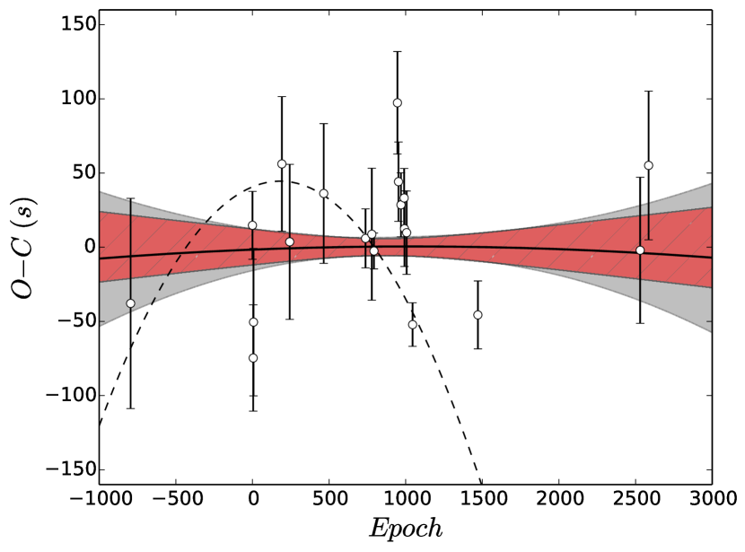
Figure 2: Updated Observed minus Calculated diagram for the transit midtimes of OGLE-TR-113b using a constant period ephemeris (eq. 2). The $\pm 1\sigma$ errors of the linear ephemeris is represented by the red-hatched region. The RMS of the residuals is 42 seconds. The linearly changing period ephemeris (eq. 3) is represented by the solid black line and its $\pm 1\sigma$ errors by the gray region. The dashed line represents the corrected changing period function reported by Adams et al. 2010.

Fit	Period	$T_{0}$	$\delta P$	$\dot{P}$	$\chi^{2}$	$\chi^{2}_{red}$	$BIC$	$RMS$
	(days)	(BJDTDB)	($\times 10^{-10}$ days)	($ms~{}yr^{-1}$)				(seconds)
Linear	1.43247506(14)	2453464.61708(14)	–	–	42	2.3	48	42
Quadratic	1.43247510(28)	2453464.61706(16)	$-0.5\pm 2.5$	$-1.0\pm 6.0$	42	2.5	51	41

Table 5: Results of the linear and quadratic fits of the transit times of OGLE-TR-113b.

5 Perturber Mass Limits

Using the limits imposed by our TTV analysis ($RMS=42$ seconds) we investigate the mass of additional perturbing bodies in the system, which could produce the observed dispersion in the transit midtimes. For this, we use the Mercury integrator code (Chambers, 1999) to generate a set of dynamical simulations of the OGLE-TR-113 system. We use circular and coplanar orbits and set the physical properties of the star and OGLE-TR-113b to the values listed in Table 2. The initial orbit of the perturber was calculated from Kepler’s third law by using an orbital period in the range $P_{per}=0.1-4.5P_{tran}$ in steps of $0.05$ or $0.005~{}P_{tran}$ when more resolution was needed, e.g. near Mean Motion Resonances (MMRs). $P_{tran}$ is the OGLE-TR-113b orbital period derived in this work. The perturber mass varied from $0.1$ to $1500$ $M_{\oplus}$; this variation depends on the calculated TTV (see below). We let the system evolve for 15 years but we save transit times only after the first 3 years to avoid any perturbation induced by initial conditions. For each simulation we imposed the condition that the calculated period of the transiting planet did not deviate more than $60$ seconds from the real period of OGLE-TR-113b. If the deviation was larger then the initial conditions of the transiting planet’s orbit for that specific simulation were changed in order to obtain the desired orbital period. Usually small changes in the initial location of the planet were necessary. Then, for each simulation the $RMS$ of the TTVs was calculated, increasing the perturber mass until an $RMS=45$ seconds was reached. Close to this mass level, we ran again the simulations using a mass step of $0.1$ or $1.0$ $M_{\oplus}$, depending on the required precision. The results of these dynamical simulations are shown in Figure 3. By using the limits of our timing analysis we discard perturbers with masses larger than 0.5 and 0.9 $M_{\oplus}$ near the 1:2 and 5:3 MMRs, 1.2 $M_{\oplus}$ near the 2:1 MMR and 3.0 $M_{\oplus}$ near the 3:1 MMR. While we agree with the mass limits placed by A10 in the 1:2 and 2:1 MMRs, our 5:3 and 3:1 MMR limits are almost one order of magnitude more strict.

Figure 3: Mass as a function of its orbital period of a hypothetical perturber in the OGLE-TR-113 system. The gray strip and vertical lines represent the instability region of the system and the location of the principal Mean Motion Resonances, respectively.

6 Conclusions

We have observed nine new transits of OGLE-TR-113b as part of TraMoS project extending the time span of the observations from 6 years to over 13 years. By performing a simultaneous timing analysis of these transits and literature transits we tested the tentative detection of orbital period decay for this planet reported by Adams et al. (2010).

Our timing analysis of 20 transit epochs discards the presence of a linearly changing period of OGLE-TR-113b. We obtain a $\delta P=(-0.5\pm 2.5)\times 10^{-10}$ days which is fully consistent with a constant orbital period for OGLE-TR-113b. Our updated $\dot{P}=-1.0\pm 6.0$ ms yr^-1 is about 1 order of magnitude smaller than the value reported by A10 and consistent with zero.

For a large sample of Kepler planet hosts, Penev et al. (2012) set a strong limit on the tidal quality factor of $Q_{\star}\geq 10^{7}$. In the case of OGLE-TR-113b, using a $1\sigma$ value based on our measured orbital decay, i.e. $\dot{P}=-7.0$ ms yr^-1, stellar and planetary masses from Southworth (2012), and eqs. 5 and 7 from Birkby et al. (2014) we obtain $Q_{\star}\sim 2.6\times 10^{4}$ for this sytem. Those values of $Q_{\star}$ imply a $T_{shift}=157$ seconds after 13.2 years, which is clearly not observed in the $O-C$ diagram in Figure 2. Using $\dot{P}=-1.0$ ms yr^-1, we obtain $Q_{\star}\sim 1.8\times 10^{5}$ and a $T_{shift}$ of $22$ seconds, which is fully consistent with the RMS of the timing residuals. Therefore, based on our timing analysis we can discard $Q_{\star}<10^{5}$. A time shift of 100 seconds is expected in 7 more years (i.e. in a total of 20 years of monitoring) if $Q_{\star}\sim 10^{5}$ and $\dot{P}$ is of only a few ms yr^-1. Only a 10 seconds shift is expected if $Q_{\star}\sim 10^{6}$ instead. Additionally, based also on the timing analysis of the transits, we can place strict constraints on the mass of additional bodies in the system. We discard planets with masses larger than 0.5, 0.9, 1.2 and 3.0 $M_{\oplus}$ near the 1:2, 5:3, 2:1 and 3:1 MMRs. Finally, with the homogeneous analysis of these data and the literature transits, we update the physical properties of this system.

7 Acknowledgements

We thank the anonymous referee for the useful comments that helped to improve the quality of the manuscript and R. Alonso for helpful discussion.

Based on observations obtained at the Gemini Observatory, which is operated by the Association of Universities for Research in Astronomy, Inc., under a cooperative agreement with the NSF on behalf of the Gemini partnership: the National Science Foundation (United States), the National Research Council (Canada), CONICYT (Chile), the Australian Research Council (Australia), Ministério da Ciência, Tecnologia e Inovação (Brazil) and Ministerio de Ciencia, Tecnología e Innovación Productiva (Argentina).

Based on observations obtained at the Southern Astrophysical Research (SOAR) telescope, which is a joint project of the Ministério da Ciência, Tecnologia, e Inovação (MCTI) da República Federativa do Brasil, the U.S. National Optical Astronomy Observatory (NOAO), the University of North Carolina at Chapel Hill (UNC), and Michigan State University (MSU).

S.H. acknowledges financial support from the Spanish Ministry of Economy and Competitiveness (MINECO) under the 2011 Severo Ochoa Program SEV-2011-0187. PR acknowledges Fondecyt #1120299, Anillo ACT1120. DM is supported by the Millennium Institute of Astropysics MAS from the Ministry of Economy ICM grant P07-021-F. PR and DM are also supported by the BASAL CATA Center for Astrophysics and Associated Technologies PFB-06.

References

- Adams et al. (2010) Adams E. R., López-Morales M., Elliot J. L., Seager S., Osip D. J., 2010, ApJ, 721, 1829
- Agol et al. (2005) Agol E., Steffen J., Sari R., Clarkson W., 2005, MNRAS, 359, 567
- Anderson & Darling (1954) Anderson T. W., Darling D. A., 1954, JASA, 49, 765
- Birkby et al. (2014) Birkby J. L. et al., 2014, MNRAS, 440, 1470
- Bouchy et al. (2004) Bouchy F., Pont F., Santos N. C., Melo C., Mayor M., Queloz D., Udry S., 2004, A&A, 421, L13
- Carone & Pätzold (2007) Carone L., Pätzold M., 2007, P&SS, 55, 643
- Carter & Winn (2009) Carter J. A., Winn J. N., 2009, ApJ, 704, 51
- Chambers (1999) Chambers J. E., 1999, MNRAS, 304, 793
- Csizmadia et al. (2012) Csizmadia S., Pasternacki T., Dreyer C., Cabrera J., Erikson A., Rauer H., 2012, A&A, 549, A9
- Diaz et al. (2007) Diaz R. F. et al., 2007, ApJ, 660, 850
- Eastman et al. (2010) Eastman J., Siverd R., Gaudi B. S., 2010, PASP, 122, 935
- Foreman-Mackey et al. (2013) Foreman-Mackey D., Hogg D. W., Lang D., Goodman J., 2013, PASP, 125, 306
- Gazak et al. (2012) Gazak J. Z., Johnson J. A., Tonry J., Dragomir D., Eastman J., Mann A. W., Agol E., 2012, Adv.Astron., 2012, 30
- Gillon et al. (2006) Gillon M., Pont F., Moutou C., Bouchy F., Courbin F., Sohy S., Magain P., 2006, A&A, 459, 249
- Holman & Murray (2005) Holman M. J., Murray N. W., 2005, Science, 307, 1288
- Hoyer et al. (2013) Hoyer S. et al., 2013, MNRAS, 434, 46
- Hoyer et al. (2012) Hoyer S., Rojo P., López-Morales M., 2012, ApJ, 748, 22
- Hoyer et al. (2011) Hoyer S., Rojo P., López-Morales M., Díaz R. F., Chambers J., Minniti D., 2011, ApJ, 733, 53
- Konacki et al. (2004) Konacki M. et al., 2004, ApJL, 609, L37
- Levrard et al. (2009) Levrard B., Winisdoerffer C., Chabrier G., 2009, ApJL, 692, L 9
- Matsumura et al. (2010) Matsumura S., Peale S. J., Rasio F. A., 2010, ApJ, 725, 1995
- Miralda-Escudé (2002) Miralda-Escudé J., 2002, ApJ, 564, 1019
- Pätzold et al. (2004) Pätzold M., Carone L., Rauer H., 2004, A&A, 427, 1075
- Penev et al. (2012) Penev K., Jackson B., Spada F., Thom N., 2012, ApJ, 751, 96
- Penev & Sasselov (2011) Penev K., Sasselov D., 2011, ApJ, 731, 67
- Pietrukowicz et al. (2010) Pietrukowicz P. et al., 2010, A&A, 509, A4
- Sasselov (2003) Sasselov D. D., 2003, ApJ, 596, 1327
- Snellen & Covino (2007) Snellen I. A. G., Covino E., 2007, MNRAS, 375, 307
- Southworth (2012) Southworth J., 2012, MNRAS, 426, 1291
- Udalski et al. (2002) Udalski A., Szewczyk O., Zebrun K., Pietrzynski G., Szymanski M., Kubiak M., Soszynski I., Wyrzykowski L., 2002, ACA, 52, 317