Interacting spin-orbit-coupled spin-1 Bose-Einstein condensates

Abstract

The recent experimental realization of spin-orbit (SO) coupling for spin-1 ultracold atoms opens an interesting avenue for exploring SO-coupling-related physics in large-spin systems, which is generally unattainable in electronic materials. In this paper, we study the effects of interactions between atoms on the ground states and collective excitations of SO-coupled spin-1 Bose-Einstein condensates (BECs) in the presence of a spin-tensor potential. We find that ferromagnetic interaction between atoms can induce a stripe phase exhibiting in-phase or out-of-phase modulating patterns between spin-tensor and zero-spin-component density waves. We characterize the phase transitions between different phases using the spin-tensor density as well as the collective dipole motion of the BEC. We show that there exists a double maxon-roton structure in the Bogoliubov-excitation spectrum, attributed to the three band minima of the SO-coupled spin-1 BEC.

I Introduction

Ultracold atoms have become a versatile platform for exploring quantum matter in the presence of a variety of gauge fields Dalibard2011 ; Galitski2013 ; Goldman2014 . One important breakthrough in this direction is the recent experimental synthesis of coupling between a particle’s spin and linear momentum, or spin-orbit (SO) coupling, for pseudo-spin-half ultracold atoms Lin2011 ; Zhang2012b ; Qu2013a ; Olson2014 ; Hamner2014 ; Wang2012 ; Cheuk2012 ; Williams2013 ; Huang2015 via the light–atom interaction Higbie2002 ; Spielman2009 . Such synthetic SO coupling emulates the Rashba and Dresselhaus SO coupling for electrons in solids that plays a crucial role for many condensed-matter phenomena Xiao2010 ; Qi2011 . Because of the coupled spin and momentum, many interesting and exotic SO-coupling-related phenomena have been theoretically proposed and experimentally observed Stanescu2008 ; Wang2010 ; Wu2011 ; Ho2011 ; Zhang2012a ; Hu2012 ; Ozawa2012 ; Li2012a ; Gong2011 ; Hu2011 ; Yu2011 ; Qu2013b ; Zhang2013b ; Lin14 .

While electrons have spin-half, pseudospin of atoms, defined by their hyperfine states, could have higher spins. For instance, spin-1 Bose-Einstein condensates (BECs) have been widely studied in ultracold atomic gases Ho1998 ; Ohmi1998 ; Stenger1998 ; Stamper-Kurn2013 . In this context, the recent experimental realization of SO coupling for spin-1 BECs through Raman coupling among three hyperfine states Campbell2015 (see Fig. 1) or with the use of a gradient magnetic field Luo2015 provides an interesting avenue for exploring SO-coupling-related physics in high-spin systems. In the experiment of Ref. Campbell2015 , the SO coupling is generated together with tunable transverse-Zeeman and spin-tensor potentials. While the transverse-Zeeman potential plays the same role as in the spin-half system Higbie2002 ; Spielman2009 —to topologically change the band structure by opening a gap, the spin-tensor potential has fundamentally different rotation properties and acts only in spin-1 (or higher-spin) space. Therefore, the system enables exploration of spin-tensor-related physics in the SO-coupled superfluid. The interplay between SO coupling and both potentials leads to a rich single-particle band structure Lan2014 , which characterizes quantum phases with itinerant magnetism and different types of phase transitions that have been experimentally observed Campbell2015 . However, interaction effects on both ground state phase diagrams and collective excitations in such spin-1 system have been largely unexplored.

In this paper, we study the effects of density-density and spin-spin interactions, two natural elements in spinor BECs Ho1998 , on the ground-state phase diagrams and elementary excitations. Our results are based on the variational-wavefunction approach and numerical simulation of Gross-Pitaevskii equation (GPE), which agree with each other. The main results are as follows:

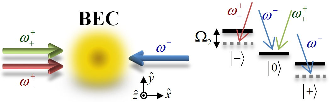
Figure 1: (Color online) Left: The scheme to generate SO coupling in a spin-1 BEC with three Raman lasers. Right: Raman transitions between three hyperfine states with detuning $\Omega_{2}$, which controls the spin-tensor potential.

(1) The ground-state phase diagrams are obtained for different parameters. Particularly, there exists an interaction-induced stripe phase exhibiting in-phase or out-of-phase modulations between spin-tensor and zero-spin-component density waves. The size of the stripe-phase region is proportional to the ferromagnetic interaction. The stripe phase is the coherent superposition of components from three band minima and possesses both crystalline and superfluid properties, resembling the supersolid phases Pomeau1994 .

(2) The phase transitions (transition order and change of properties) are characterized using the spin-tensor density, the time-of-flight momentum distribution, and the period of collective dipole motions of the system.

(3) We reveal rich roton phenomena in the Bogoliubov-excitation spectrum, including symmetric/asymmetric double-roton structures and the roton gap closing at the stripe-phase boundary. Such double-roton structures have not been found in widely studied superfluids such as liquid ⁴He Ozeri2005 ; Leggett2006 , BECs with long range interactions Lahaye2009 ; Mottl2012 , and SO-coupled spin-half BECs Khamehchi2014 ; Ji2015 ; Ha2015 , which possess single-roton excitations.

II Model and Hamiltonian

As illustrated in Fig. 1, we consider the experimental scheme of Ref. Campbell2015 , which employs three Raman lasers with wave vector $k_{\mathrm{R}}$ to generate SO coupling in a spin-1 BEC. The pair of counterpropagating beams $\omega_{-}$ and $\omega_{+}^{+}$ ($\omega_{-}^{+}$) induces a two-photon Raman transition between two atomic hyperfine states $|0\rangle$ and $|+\rangle$ ($|-\rangle$) and imparts 2$k_{\mathrm{R}}$ recoil momentum to the atoms. Following similar discussion and modeling for the system at the single-particle level in Refs. Campbell2015 ; Lan2014 ; Campbell2015b , we consider the noninteracting Hamiltonian in pseudo-spin-1 basis $\Psi={\left({\begin{array}[]{ccc}{\psi_{+}}&{\psi_{0}}&{\psi_{-}}\end{array}}\right)^{T}}$ as

$$\tilde{H}_{0}=-\frac{{{\hbar^{2}}{\nabla^{2}}}}{{2m}}+{{\mathbf{\tilde{\Omega}}}_{\mathbf{1}}}(x)\cdot\mathbf{F}+{{\tilde{\Omega}}_{2}}F_{z}^{2},$$ (1)

where an effective magnetic field ${{\mathbf{\tilde{\Omega}}}_{\mathbf{1}}}(x)={{\tilde{\Omega}}_{1}}[\cos(2k_{\mathrm{R}}x)\hat{x}-\sin(2k_{\mathrm{R}}x)\hat{y}]$, associated with the beam intensity, couples to the hyperfine states represented by spin-1 Pauli matrices $\mathbf{F}={\left({\begin{array}[]{ccc}{F_{x},}&{F_{y},}&{F_{z}}\end{array}}\right)}$, $\tilde{\Omega}_{2}$ is an effective detuning for $|\pm\rangle$ (hence taking a spin-tensor form $F_{z}^{2}$), and $m$ is the atomic mass. Since ${{\mathbf{\tilde{\Omega}}}_{\mathbf{1}}}(x)$ has effects only in the spatial $x$ direction, one can assume that the ground-state wavefunction in the $y$ and $z$ directions remains the case without it. After unitary transformation $\psi_{\pm}\rightarrow\psi_{\pm}e^{\pm 2ik_{\mathrm{R}}x}$ and integration over $y$ and $z$ degrees of freedom, we obtain a Hamiltonian in momentum and energy units $\hbar k_{\mathrm{R}}$ and $\hbar^{2}k_{\mathrm{R}}^{2}/2m$, respectively, as

$$H_{0}=-\partial_{x}^{2}-4i{\partial_{x}}\otimes{F_{z}}+({\Omega_{2}}+4)F_{z}^{2}+{\Omega_{1}}{F_{x}},$$ (2)

where $\Omega_{1,2}$ are dimensionless variables controlling the transverse-Zeeman and spin-tensor potentials, respectively. The term $-i\partial_{x}\otimes F_{z}=p_{x}\otimes F_{z}$ represents the spin–linear-momentum coupling.

The ground-state properties of $H_{0}$ can be characterized by considering the minima in the lowest energy band,

$${E_{k}}={k^{2}}-\sqrt[{}^{3}]{{A}_{k}^{\prime}/54}-{A_{k}}\sqrt[{}^{3}]{2/(27{{\ A_{k}^{\prime}}})}+2{A_{0}/3},$$ (3)

where $A_{0}=\Omega_{2}+4$, ${A_{k}}=48{k^{2}}+A_{0}^{2}+3\Omega_{1}^{2}$, and ${A_{k}^{\prime}}={A_{0}}{A_{k}^{\prime\prime}}+\sqrt{-4A_{k}^{3}+{A_{0}^{2}}{{A_{k}^{\prime\prime}}^{2}}}$ with ${A_{k}^{\prime\prime}}=-288{k^{2}}+2A_{0}^{2}+9\Omega_{1}^{2}$. The structure of $E_{k}$ can exhibit (A) one local minimum at $k=0$ [right inset in Fig. 2 (a)], (B) two at $k=\pm k_{0}\neq 0$ (bottom inset), or (C) three at $k=0,\pm k_{0}$ (top two insets) as $\Omega_{1,2}$ vary. The ground state always stays at $k=0$ in the region $\Omega_{2}>0$ and can undergo a phase transition between $0$ and $\pm k_{0}$ in $\Omega_{2}\leq 0$. Along the phase boundary in the $\Omega_{1}$-$\Omega_{2}$ plane, there is a triple point $(\Omega_{1}^{\ast},\Omega_{2}^{\ast})$ that separates two types of transitions: a first-order transition in $\Omega_{1}<\Omega_{1}^{\ast}$ upon which structure (C) remains and $k$ suddenly jumps (top two insets) and a second-order transition upon which the structure evolves between (A) and (B) and $k$ continuously changes (bottom two insets). The boundaries of first-order and second-order transitions meet the conditions $E_{0}=E_{\pm k_{0}}$ and $\partial_{k}^{2}E_{0}=0$, respectively, which represent a monotonically decreasing curve in the $\Omega_{1}$-$\Omega_{2}$ plane. The triple point takes place at the merging of the three local minima $\pm k_{0}\rightarrow 0$ of structure (C), which gives $(\Omega_{1}^{\ast},\Omega_{2}^{\ast})=(4.805,-1.666)$ and a flat low-energy behavior $E_{k}\sim 0.0165k^{6}$ Triple_point .

III Variational calculation

For a realistic BEC, the energy density of the system can be expressed as

$$\varepsilon=\frac{1}{V}\int{dx{\Psi^{{\dagger}}}\left[{{H_{0}}+\frac{{c_{0}}}{2}{\Psi^{{\dagger}}}\Psi+\frac{{c_{2}}}{2}\left({{\Psi^{{\dagger}}}\mathbf{F}\Psi}\right)\cdot\mathbf{F}}\right]\Psi},$$ (4)

where $V$ is the system volume and $c_{0,2}$ describe density-density and spin-spin interaction strengths. The wave function is normalized as $V^{-1}\int{dx{\Psi^{{\dagger}}}\Psi}=1$ such that $c_{0,2}$ are proportional to the particle density $N/V$. Note that $c_{0,2}$ could also be tuned through Feshbach resonances Chin10 . To obtain the ground state, we adopt a variational ansatz,

$$\Psi=\left|{C_{0}}\right|{\chi_{0}}+\sum\nolimits_{s=\pm}{\left|{C_{s}}\right|{\chi_{s}}{e^{is(kx+{\alpha_{s}})}}},$$ (5)

where the spin components are of the form ${\chi_{-}}(\theta,\phi)={\left({\begin{array}[]{ccc}{\cos\theta\cos\phi}&{\ -\sin\theta}&{\cos\theta\sin\phi}\end{array}}\right)^{T}}$, ${\chi_{0}}={\chi_{-}}(\frac{\pi}{2}-\theta^{\prime},\frac{\pi}{4})$, and ${\chi_{+}}={\chi_{-}}(\theta,\frac{\pi}{2}-\phi)$. The normalization condition gives $\sum\nolimits_{s=0,\pm}{{{\left|{C_{s}}\right|}^{2}}}=1$. Inserting Eq. (5) into Eq. (4), we obtain $\varepsilon$ as a functional of seven variational parameters $k$, $|C_{\pm}|$, $\theta$, $\theta^{\prime}$, $\phi$, and $\alpha=\alpha_{-}-\alpha_{+}$ (see Appendix A), which are generally different from their single-particle values Lan2014 ; Natu2015 . The ground state is computed through the minimization of $\varepsilon$. We also calculate the ground state by solving the GPE using imaginary time evolution and find good agreement between both methods.

In terms of the variational variables, we obtain the spin polarization $\left\langle{F_{z}}\right\rangle=({\left|{C_{+}}\right|^{2}}-{\left|{C_{-}}\right|^{2}}){\cos^{2}}\theta\cos 2\phi$ and spin tensor $\left\langle{F_{z}^{2}}\right\rangle=({\left|{C_{+}}\right|^{2}}+{\left|{C_{-}}\right|^{2}})\cos^{2}\theta+{\left|{C_{0}}\right|^{2}}{\sin^{2}}\theta^{\prime}$, which are directly related to the spin-resolved density profiles ${V^{-1}}\int{dx({{\rho_{+}}\mp{\rho_{-}}})}$ with $\rho_{s}=|\psi_{s}|^{2}$, respectively, and can hence be measured in the time-of-flight experiment. The minimization of energy with respect to $k$, i.e., $\partial\varepsilon/\partial k=0$, leads to the ground-state spin polarization associated with momentum $\langle{F_{z}}\rangle=-\frac{k}{2}({\left|{C_{+}}\right|^{2}}-{\left|{C_{-}}\right|^{2}})$, which is a result of SO coupling.

IV Interacting phase diagram

The variational ansatz characterizes three quantum phases: (I) the uniform phase with a constant wavefunction at $k=0$, and hence $\langle{F_{z}}\rangle=0$; (II) the plane-wave phase with $k\neq 0$, one of $|C_{\pm}|$ equal to $1$, and hence $\langle{F_{z}}\rangle\neq 0$; and (III) the stripe phase with $k\neq 0$ and at least two of $|C_{0,\pm}|$ are not $0$. The plane-wave phase has two degenerate states with opposite momentum and hence opposite spin polarization. Below we present only the positively polarized plane-wave state for convenience. The stripe phase exhibits spatial density modulation $\rho(x)=\sum\nolimits_{s=0,\pm}\rho_{s}$ with periods determined by the superposition of the uniform and plane-wave states. The transition between phases is first order (second order) if $\frac{\partial\varepsilon}{\partial\Omega_{2}}=\langle F_{z}^{2}\rangle$ ($\frac{\partial^{2}\varepsilon}{\partial\Omega_{2}^{2}}=\frac{\partial\langle F_{z}^{2}\rangle}{\partial\Omega_{2}}$) Hellmann-Feynman displays discontinuity as $\Omega_{2}$ varies across the phase boundary. Another polarization $\langle F_{x}\rangle=\frac{\partial\varepsilon}{\partial\Omega_{1}}$ can also indicate the type of phase transitions but is less experimentally accessible. Note that the behavior of $\langle F_{z}\rangle$ is not directly related to the energy derivatives in the $\Omega_{1}$-$\Omega_{2}$ plane. In fact it can not tell the transition involving the stripe phase, as we will show later.

Figure 2(a) shows the ground-state phase diagram in the $\Omega_{1}$-$\Omega_{2}$ plane at $(c_{0},c_{2})=(5,-0.1)$. Outside the small framed region, we find that such small spin-spin interaction $c_{2}$ has little effects on the phase diagram. The quantum phases and phase transitions can still be well described by the single-particle energy band (see insets), except that the system always stays in one of the minima given the degeneracy due to the density-density interaction $c_{0}$, in contrast to the noninteracting ground state, which can be arbitrary superposition of degenerate minima. As a result, the boundaries of first-order (solid curve) and second-order (dashed) transitions between the uniform (I) and plane-wave (II) phases as well as the place of triple point (star sign) show indiscernible difference from the noninteracting case. When $c_{2}$ becomes stronger to $-2$, it enlarges region II but does not qualitatively change the I–II boundary.

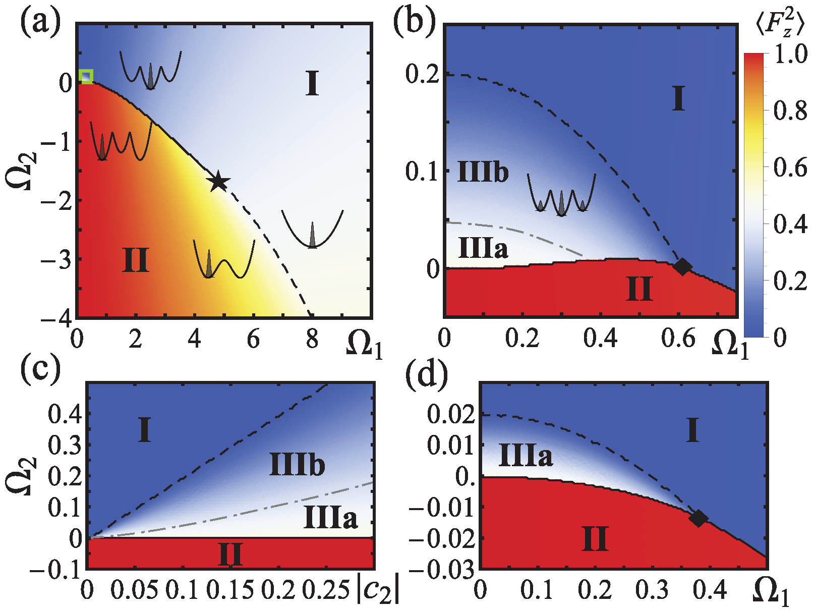
Figure 2: (Color online) (a) Ground-state phase diagram in the $\Omega_{1}$-$\Omega_{2}$ plane for $(c_{0},c_{2})=(5,-0.1)$. (b) Closeup of the framed region in panel (a). Regions I, II, and IIIa/IIIb, represent uniform, plane-wave, and stripe phases, respectively. The solid, dashed, and dot-dashed curves show first-order-transition, second-order-transition, and crossover boundaries, respectively. The star (diamond) sign denotes the triple (tricritical) point. The insets show schematic single-particle band structures and the BEC’s occupation in the momentum space. (c) Phase diagram in the $|c_{2}|$-$\Omega_{2}$ plane for $c_{0}=5$ and $\Omega_{1}=0.1$. (d) Phase diagram in the $\Omega_{1}$-$\Omega_{2}$ plane for $(c_{0},c_{2})=(0.5,-0.01)$.

Figure 2(b) zooms in the framed region in Fig. 2(a). We see the appearance of a stripe phase III sandwiched by I and II. The III–II and III–I transition boundaries are first order (solid curve) and second order (dashed), respectively, and meet at a tricritical point $(0.6,0.005)$ (diamond sign). The stripe phase represents co-occupancy of the three states of the form $|C_{0}|>|C_{+}|=|C_{-}|>0$ (see insets), so its direct evidence would be a symmetric three-peak structure at $0$ and $\pm k$ in the time-of-flight experiment. Such a superposition leads to spatially modulated $\rho$ and spin-tensor density $\rho_{+}+\rho_{-}$ with period $2\pi/k$, while the spin polarization $\rho_{+}-\rho_{-}=0$ remains uniform. The stripe phase shows two patterns: $\rho_{+}+\rho_{-}$ and $\rho_{0}$ have (IIIa) in-phase modulations (coincident maxima and minima) or (IIIb) out-of-phase modulations. The IIIb pattern results from a stronger interband mixing due to the interaction. The amplitude of $\rho_{0}$ smoothly suppresses to zero on the IIIa–IIIb crossover boundary (dot-dashed curve) and changes sign across the boundary.

We turn to study the effect of interaction strength on the phase boundaries. Figure 2(c) shows the phase diagram in the $|c_{2}|$-$\Omega_{2}$ plane ($c_{2}<0$ remains ferromagnetic) for $c_{0}=5$ and $\Omega_{1}=0.1$. We see that the stripe-phase region linearly increases with $|c_{2}|$. For weaker interaction $(c_{0},c_{2})=(0.5,-0.01)$, we find that IIIb disappears and the II–III boundary monotonically decreases from $\Omega_{2}=0$ as in the single-particle case [see Fig. 2(d)], but the linear increase of the stripe region with $|c_{2}|$ remains. Since $|c_{2}|$ is proportional to the average particle density, we expect the stripe phase to be more attainable in a dense system. A ⁸⁷Rb system with density $10^{15}\mathrm{{cm}^{-3}}$, $s$-wave scattering length $100.48a_{0}$ ($a_{0}$ is the Bohr radius), and Raman-laser wavelength $800$ nm corresponds to $c_{0}=2.2$ and $c_{2}=-0.01$, which predict the stripe phase within $\tilde{\Omega}_{1}<0.23E_{R}=814.2h\times\mathrm{Hz}$ and $\tilde{\Omega}_{2}<0.02E_{R}=70.8h\times\mathrm{Hz}$. For ¹³³Cs, the difference between intraspin and interspin interactions is easily tunable due to a broad Feshbach resonance of the intraspin scattering Chin10 , so $|c_{2}|$ can be enhanced without increasing the density.

To show the system behavior upon the phase transitions, we plot several observables in Fig. 3(a), including $\langle F_{z}^{2}\rangle$ (solid curve), $\langle F_{z}\rangle$ (dashed), and combined occupancy $P=|C_{+}^{2}C_{-}^{2}|\times 10$ (dot-dashed) vs $\Omega_{2}$ along path $\Omega_{1}=0.2$ in Fig. 2(b). The discontinuity in $\langle F_{z}^{2}\rangle$ [$\frac{\partial\langle F_{z}^{2}\rangle}{\partial\Omega_{2}}$ (see inset)] indicates the II–III (III–I) transition to be first (second) order. The $\langle F_{z}\rangle$ curve can also indicate the II–III transition but not III–I. The stripe phase has $\langle F_{z}\rangle=0$, the same as the uniform phase, but exhibits nonzero co-occupancy $P>0$. This underlines the insufficiency to characterize the interacting systems with only spin polarization.

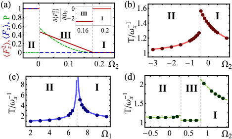
Figure 3: (Color online) (a) $\langle F_{z}^{2}\rangle$ (solid curve), $\langle F_{z}\rangle$ (dashed), and $P=10|C_{+}^{2}C_{-}^{2}|$ (dot-dashed) vs $\Omega_{2}$ along path $\Omega_{1}=0.2$ in Fig. 2(b). The inset shows $\frac{\partial\langle F_{z}^{2}\rangle}{\partial\Omega_{2}}$. (b) [(c)] Dipole oscillation periods $T$ along path $\Omega_{1}=2$ ($\Omega_{2}=-3$) across a first-order (second-order) transition. Filled circles (solid curves) are obtained from the GPE (effective-mass method). (d) $T$ across the stripe phase along path $\Omega_{1}=1.3$ (with thick-dashed fitting curves). Phases are labeled in the corresponding regions separated by dashed lines.

V Dipole oscillation

We study dipole collective modes of a trapped BEC as another experimental probe Zhang2012b for the phase transitions. We consider an experimental setup of $5\times 10^{4}$ ⁸⁷Rb atoms with the aforementioned scattering length and Raman-laser wavelength and anisotropic trapping frequencies $\omega_{x}=\omega_{y}=0.23\omega_{z}=2\pi\times 33$ Hz, producing an effective two-dimensional system in our simulation (where we integrate out only the $z$ degrees of freedom). After an initial displacement of $1.26$ $\mu$m in the $x$ direction, we compute the BEC’s periodic motion by numerically solving the time-dependent GPE and record the oscillation period $T$. In our simulation, we do not see effects of the $y$ degrees of freedom on $T$. We first study the transition between phases I and II. Figure 3(b) [(c)] shows that $T$ exhibits a discontinuity (diverges) upon the first-order (second-order) transition along path $\Omega_{1}=2$ ($\Omega_{2}=-3$) in the $\Omega_{1}$-$\Omega_{2}$ plane. Such behaviors well match the effective-mass approximation Chen2012 (see solid curves), in which the dipole motion is considered as a semi-classical simple harmonic oscillator subject to the energy dispersion $E_{k}$ of Eq. (3). The displacement $x(t)$ and momentum $k(t)$ obey the equation of motion $\partial_{t}k=-\omega_{x}^{2}x$ and $\partial_{t}x=\partial E_{k}/\partial k$, resulting in the period $T\propto\sqrt{m_{\mathrm{eff}}}$ with effective mass $m_{\mathrm{eff}}=(\partial^{2}E_{k}/\partial k^{2})^{-1}$ defined by the band curvature. Therefore, the divergence of $T$ upon the second-order transition comes from the band flatness $\partial^{2}E_{k}/\partial k^{2}=0$. By expanding the curvature around a second-order transition point $(\Omega_{1}^{c},\Omega_{2}^{c})$, we obtain the critical behavior $T\propto|\Omega_{1(2)}-\Omega_{1(2)}^{c}|^{-1/2}$ at fixed $\Omega_{2(1)}$, with the critical exponent consistent with the spin-half case Li2012b . For the stripe phase, we find that its dipole oscillation period is lower than those of the other phases. To reveal the salient feature of such a trend, we study a strongly interacting system with $(c_{0},c_{2})=(10,-2)$ in a one-dimensional trap along path $\Omega_{1}=1.3$. Figure 3(d) shows the results from the GPE calculations (the effective-mass approximation no longer fits here). We see a clear drop in the period of the stripe phase compared with the nonstripe phases, with the discontinuities matching the boundaries (dashed lines).

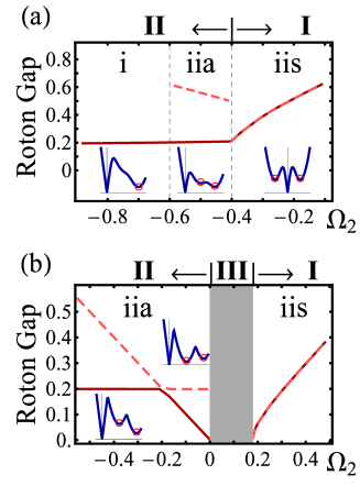
Figure 4: (Color online) (a), (b) The lowest (solid curve) and second-lowest (dashed curve) roton gaps vs $\Omega_{2}$ along paths $\Omega_{1}=2$ in Fig. 2(a) and $0.2$ in Fig. 2(b), respectively. Regions of different roton structures (see text) are labeled and separated by dashed lines. The corresponding ground-state phases are labeled above the panels. Curves in the insets show schematic Bogoliubov-excitation spectra ($x$ and $y$ axes represent momentum and energy, respectively) in the corresponding regions. The roton modes are circled. There are no roton excitations in the shaded region of the stripe phase Li2013 .

VI Double rotons

The triple-well band structure of the spin-1 BEC leads to exotic quasiparticle excitations that do not exist in previous spin-half or long-range-interacting systems. We calculate the Bogoliubov excitations for phases I and II by solving the Bogoliubov equation, derived by linearizing the GPE with plane-wave-type particle and hole perturbations (see Appendix B). We first see that the excitation spectrum is always gapless and linear in the small-momentum region, presenting typical phonon modes in BECs. In a larger-momentum region, we find a rich structure of rotons, i.e., quasistable modes with zero group velocity. In Fig. 4(a), we plot the energy gaps of the lowest and second-lowest (if present) rotons along path $\Omega_{1}=2$ in Fig. 2(a). There are two types of roton structures in phase II: (i) single roton and (iia) asymmetric double rotons. In phase I, there are symmetric and degenerate double rotons (iis) (see insets for schematic spectra with marked rotons). Therefore, the sudden change in the roton structure can be a signature for the II–I transition. Figure 4(b) shows the results along path $\Omega_{1}=0.2$. We see that when the system approaches to III from II, the two roton gaps first cross each other. Then the one at lower momentum keeps decreasing to zero at the II–III boundary, while the other remains finite. If approaching from I, the degenerate gaps both drop to zero at the I–III boundary. Such gap closing is a signature of the transition to the stripe phase, resembling to the transition to the supersolid phase that possesses both crystalline and superfluid orders. The trend of the reducing roton gap close to the stripe phase was experimentally observed previously for the spin-half system Khamehchi2014 ; Ji2015 . The Bogoliubov excitations in the stripe phase itself are more complicated and there are no rotons Li2013 (shaded region). Note that such double rotons have not been found in the previously studied superfluids Ozeri2005 ; Leggett2006 ; Lahaye2009 ; Mottl2012 ; Khamehchi2014 ; Ji2015 ; Ha2015 .

VII Summary

In summary, we have characterized the ground-state phase diagrams and collective excitations in interacting SO-coupled spin-1 BECs with spin-tensor potentials. Our results provide timely predictions for ongoing experiments exploring SO-coupling-related physics in higher-spin systems. One interesting extension would be the investigation of spin-1 BECs with recently proposed spin–orbital-angular-momentum coupling Sun2015 ; Demarco2015 ; Qu2015 , in which the strongly interacting effects might significantly enlarge the stripe-phase region.

Acknowledgements: We are grateful to P. Engels, L. Jiang, and Z.-Q. Yu for helpful discussions. This work is supported by ARO (W911NF-12-1-0334), AFOSR (FA9550-13-1-0045), and NSF (PHY-1505496).

Appendix A Variational energy functional

In this section we show details of the variational energy functional density $\epsilon$ discussed in Sec. III. We first rewrite the variational wavefunction in Eq. (5) as

$$\left({\begin{array}[]{*{20}{c}}{{\psi_{+}}}\\ {{\psi_{0}}}\\ {{\psi_{-}}}\end{array}}\right)=\left|{{C_{-}}}\right|\left({\begin{array}[]{*{20}{c}}{\cos\theta\cos\phi}\\ {-\sin\theta}\\ {\cos\theta\sin\phi}\end{array}}\right){e^{-i(kx+{\alpha_{-}})}}+\left|{{C_{0}}}\right|\left({\begin{array}[]{*{20}{c}}{\sin\theta^{\prime}/\sqrt{2}}\\ {-\cos\theta^{\prime}}\\ {\sin\theta^{\prime}/\sqrt{2}}\end{array}}\right)+\left|{{C_{+}}}\right|\left({\begin{array}[]{*{20}{c}}{\cos\theta\sin\phi}\\ {-\sin\theta}\\ {\cos\theta\cos\phi}\end{array}}\right){e^{i(kx+{\alpha_{+}})}}.$$ (18)

We then evaluate each term of the single-particle energy density using Eq. (18) as

$$\left\langle{-\partial_{x}^{2}}\right\rangle = \frac{1}{V}\int{dx}\sum\limits_{j}{{{\psi}^{*}_{j}}(-\partial_{x}^{2}){\psi_{j}}}={k^{2}}\left({{{\left|{{C_{+}}}\right|}^{2}}+{{\left|{{C_{-}}}\right|}^{2}}}\right),$$ (19)

$$\left\langle{-4i{\partial_{x}}{F_{z}}}\right\rangle = \frac{1}{V}\int{dx}(-4i)({{\psi}^{*}_{+}}{\partial_{x}}{\psi_{+}}-{{\psi}^{*}_{-}}{\partial_{x}}{\psi_{-}})=-4k{\cos^{2}}\theta\cos 2\phi\left({{{\left|{{C_{+}}}\right|}^{2}}+{{\left|{{C_{-}}}\right|}^{2}}}\right),$$ (20)

$$\left\langle{F_{z}^{2}}\right\rangle = \frac{1}{V}\int{dx\left({{{\left|{{\psi_{+}}}\right|}^{2}}+{{\left|{{\psi_{-}}}\right|}^{2}}}\right)}=\left({{{\left|{{C_{+}}}\right|}^{2}}+{{\left|{{C_{-}}}\right|}^{2}}}\right){\cos^{2}}\theta+{\left|{{C_{0}}}\right|^{2}}{\sin^{2}}\theta^{\prime},$$ (21)

$$\left\langle{{F_{x}}}\right\rangle = \frac{1}{V}\int{dx\frac{1}{{\sqrt{2}}}\left({\psi_{+}^{\dagger}{\psi_{0}}+\psi_{0}^{\dagger}{\psi_{-}}+{\rm{H}}{\rm{.c}}{\rm{.}}}\right)}=-\left({{{\left|{{C_{+}}}\right|}^{2}}+{{\left|{{C_{-}}}\right|}^{2}}}\right)\sin 2\theta\sin\left({\phi+\frac{\pi}{4}}\right)-{\left|{{C_{0}}}\right|^{2}}\sin 2\theta^{\prime},$$ (22)

and obtain

$${\varepsilon_{0}}=\left\langle{-\partial_{x}^{2}-4i{\partial_{x}}{F_{z}}}\right\rangle+({\Omega_{2}}+4)\left\langle{F_{z}^{2}}\right\rangle+{\Omega_{1}}\left\langle{{F_{x}}}\right\rangle.$$ (23)

For the interaction energy, we have

$${\varepsilon_{{c_{0}}}} = \frac{{{c_{0}}}}{2}\frac{1}{V}\int{dx{{\left({{{\left|{{\psi_{+}}}\right|}^{2}}+{{\left|{{\psi_{0}}}\right|}^{2}}+{{\left|{{\psi_{-}}}\right|}^{2}}}\right)}^{2}}}=\frac{{{c_{0}}}}{2}\Bigg{\{}1+2{\left|{{C_{0}}}\right|^{2}}{\left[{\cos\theta\sin\theta^{\prime}\sin\left({\phi+\frac{\pi}{4}}\right)+\sin\theta\cos\theta^{\prime}}\right]^{2}}\times$$ (24)

$$\left({{{\left|{{C_{+}}}\right|}^{2}}+2\left|{{C_{+}}}\right|\left|{{C_{-}}}\right|\cos\alpha+{{\left|{{C_{-}}}\right|}^{2}}}\right)+2{\left|{{C_{+}}}\right|^{2}}{\left|{{C_{-}}}\right|^{2}}{\left({{{\cos}^{2}}\theta\sin 2\phi+{{\sin}^{2}}\theta}\right)^{2}}\Bigg{\}},$$

$${\varepsilon_{{c_{2}}}}=\frac{{{c_{2}}}}{2}\frac{1}{V}\int{dx\sum\limits_{s=x,y,z}{{{\left({\sum\limits_{ij=+,0,-}{{{\psi}^{*}_{i}}{F_{s,ij}}{\psi_{j}}}}\right)}^{2}}}}=\frac{{{c_{2}}}}{2}\frac{1}{V}\int{dx\left[{2{{\left|{{{\psi}^{*}_{+}}{\psi_{0}}+{{\psi}^{*}_{0}}{\psi_{-}}}\right|}^{2}}+{{\left({{{\left|{{\psi_{+}}}\right|}^{2}}-{{\left|{{\psi_{-}}}\right|}^{2}}}\right)}^{2}}}\right]},$$ (25)

with

$$\frac{1}{V}\int{dx}{\left|{{{\psi}^{*}_{+}}{\psi_{0}}+{{\psi}^{*}_{0}}{\psi_{-}}}\right|^{2}}=\frac{1}{2}{\left[{\left({{{\left|{{C_{+}}}\right|}^{2}}+{{\left|{{C_{-}}}\right|}^{2}}}\right)\sin 2\theta\sin\left({\phi+\frac{\pi}{4}}\right)+{{\left|{{C_{0}}}\right|}^{2}}\sin 2\theta^{\prime}}\right]^{2}}+{\left|{{C_{+}}}\right|^{2}}{\left|{{C_{-}}}\right|^{2}}{\sin^{2}}2\theta+$$

$${\left|{{C_{0}}}\right|^{2}}\left({{{\left|{{C_{+}}}\right|}^{2}}+{{\left|{{C_{-}}}\right|}^{2}}+2\left|{{C_{+}}}\right|\left|{{C_{-}}}\right|\cos{\alpha}}\right)\left[{{{\cos}^{2}}\theta{{\cos}^{2}}\theta^{\prime}+\frac{1}{2}\sin 2\theta\sin 2\theta^{\prime}\sin\left({\phi+\frac{\pi}{4}}\right)+{{\sin}^{2}}\theta{{\sin}^{2}}\theta^{\prime}}\right],$$ (26)

$$\frac{1}{V}\int{dx{{\left({{{\left|{{\psi_{+}}}\right|}^{2}}-{{\left|{{\psi_{-}}}\right|}^{2}}}\right)}^{2}}} = {\left({{{\left|{{C_{+}}}\right|}^{2}}-{{\left|{{C_{-}}}\right|}^{2}}}\right)^{2}}{\cos^{4}}\theta{\cos^{2}}2\phi+$$ (27)

$$2{\left|{{C_{0}}}\right|^{2}}{\cos^{2}}\theta{\sin^{2}}\theta^{\prime}{\cos^{2}}\left({\phi+\frac{\pi}{4}}\right)\left({{{\left|{{C_{+}}}\right|}^{2}}-2\left|{{C_{+}}}\right|\left|{{C_{-}}}\right|\cos{\alpha}+{{\left|{{C_{-}}}\right|}^{2}}}\right).$$

Combining Eqs. (23)–(27), we obtain the energy functional density $\varepsilon=\varepsilon_{0}+\varepsilon_{c_{0}}+\varepsilon_{c_{2}}$.

Appendix B Bogoliubov excitations

In this section we derive the equation for the Bogoliubov excitations discussed in Sec. VI. The dynamics of a BEC in the plane-wave or uniform phase is governed by the time-dependent Gross-Pitaevskii equation

$$i\partial_{t}\Psi(x,t)=(H_{0}+H_{\rm{int}})\Psi(x,t),$$ (28)

where $H_{0}$ is the single-particle Hamiltonian in Eq. (2), $\Psi(x,t)=(\psi_{+},\psi_{0},\psi_{-})^{T}$, and the interaction part $H_{\rm{int}}={c_{0}}{\Psi^{{\dagger}}}\Psi+{c_{2}}\left({{\Psi^{{\dagger}}}\mathbf{F}\Psi}\right)\cdot\mathbf{F}$. To calculate the Bogoliubov spectrum of the plane wave superfluids, we suppose

$$\Psi(x,t)=e^{ikx-i\mu t}(\chi^{(0)}+u_{q}e^{iqx-\omega t}+v_{q}^{*}e^{-iqx+i\omega t}),$$ (29)

where $e^{ikx}\chi^{(0)}=e^{ikx}(\chi^{(0)}_{+},\chi^{(0)}_{0},\chi^{(0)}_{-})^{T}$ is the ground state of the system and $u_{q}$ and $v_{q}$ are the wave functions with three components. Plugging Eq. (29) into Eq. (28) yields (only keeping linear terms with respect to $u_{q}$ and $v_{q}$)

$$\hbar\omega\left(\begin{array}[]{c}{u_{q}}\\ {v_{q}}\end{array}\right)=\sigma_{z}\mathcal{M}\left(\begin{array}[]{c}{u_{q}}\\ {v_{q}}\end{array}\right),$$ (34)

where $\sigma_{z}$ is the $z$-component $2\times 2$ Pauli matrix, and

$$\mathcal{M}=\left(\begin{array}[]{cc}H_{0}[\hat{p}\rightarrow(k+q)]-\mu+H_{1}&H_{2}\\ H_{2}^{*}&H_{0}^{*}[\hat{p}\rightarrow(k-q)]-\mu+H_{1}^{*}\end{array}\right),$$ (37)

with

$$H_{1} =\left(\begin{array}[]{cc}c_{0}(\rho_{0}^{(0)}+|\chi_{+}^{(0)}|^{2})+c_{2}(\rho_{z}^{(0)}+|\chi_{+}^{(0)}|^{2}+|\chi_{0}^{(0)}|^{2})&c_{0}\chi_{0}^{(0)*}\chi_{+}^{(0)}+c_{2}(\chi_{+}^{(0)}\chi_{0}^{(0)*}+2\chi_{0}^{(0)}\chi_{-}^{(0)*})\\ c_{0}\chi_{+}^{(0)*}\chi_{0}^{(0)}+c_{2}(\chi_{+}^{(0)*}\chi_{0}^{(0)}+2\chi_{0}^{(0)*}\chi_{-}^{(0)})&c_{0}(\rho_{0}^{(0)}+|\chi_{0}^{(0)}|^{2})+c_{2}(|\chi_{+}^{(0)}|^{2}+|\chi_{-}^{(0)}|^{2})\\ (c_{0}-c_{2})\chi_{+}^{(0)*}\chi_{-}^{(0)}&c_{0}\chi_{0}^{(0)*}\chi_{-}^{(0)}+c_{2}(2\chi_{+}^{(0)*}\chi_{0}^{(0)}+\chi_{0}^{(0)*}\chi_{-}^{(0)})\end{array}\right.$$ (41)

$$\left.\begin{array}[]{c}(c_{0}-c_{2})\chi_{+}^{(0)}\chi_{-}^{(0)*}\\ c_{0}\chi_{-}^{(0)*}\chi_{0}^{(0)}+c_{2}(2\chi_{+}^{(0)}\chi_{0}^{(0)*}+\chi_{0}^{(0)}\chi_{-}^{(0)*})\\ c_{0}(\rho_{0}^{(0)}+|\chi_{-}^{(0)}|^{2})+c_{2}(|\chi_{-}^{(0)}|^{2}+|\chi_{0}^{(0)}|^{2}-\rho_{z}^{(0)})\end{array}\right),$$ (45)

$$H_{2} =\left(\begin{array}[]{ccc}(c_{0}+c_{2})\chi_{+}^{(0)2}&(c_{0}+c_{2})\chi_{0}^{(0)}\chi_{+}^{(0)}&(c_{0}-c_{2})\chi_{+}^{(0)}\chi_{-}^{(0)}+c_{2}\chi_{0}^{(0)2}\\ (c_{0}+c_{2})\chi_{+}^{(0)}\chi_{0}^{(0)}&c_{0}\chi_{0}^{(0)2}+2c_{2}\chi_{+}^{(0)}\chi_{-}^{(0)}&(c_{0}+c_{2})\chi_{-}^{(0)}\chi_{0}^{(0)}\\ (c_{0}-c_{2})\chi_{+}^{(0)}\chi_{-}^{(0)}+c_{2}\chi_{0}^{(0)2}&(c_{0}+c_{2})\chi_{0}^{(0)}\chi_{-}^{(0)}&(c_{0}+c_{2})\chi_{-}^{(0)2}\end{array}\right).$$ (49)

The Bogoliubov excitation spectrum $\omega$ with respect to $q$ is numerically obtained by diagonalizing $\sigma_{z}\mathcal{M}$ (note that only the physical branches of the excitations are considered).

References

• (1) J. Dalibard, F. Gerbier, G. Juzeliūnas, and P. Öhberg, Colloquium: Artificial gauge potentials for neutral atoms, Rev. Mod. Phys. 83, 1523 (2011).
• (2) V. Galitski and I. B. Spielman, Spin-orbit coupling in quantum gases, Nature (London) 495, 49 (2013).
• (3) N. Goldman, G. Juzeliūnas, P. Öhberg, and I. B. Spielman, Light-induced gauge fields for ultracold atoms, Rep. Prog. Phys. 77, 126401 (2014).
• (4) Y.-J. Lin, K. Jiménez-García, and I. B. Spielman, Spin-orbit-coupled Bose-Einstein condensates, Nature (London) 471, 83 (2011).
• (5) J.-Y. Zhang, S.-C. Ji, Z. Chen, L. Zhang, Z.-D. Du, B. Yan, G.-S. Pan, B. Zhao, Y.-J. Deng, H. Zhai, S. Chen, and J.-W. Pan, Collective Dipole Oscillations of a Spin-Orbit Coupled Bose-Einstein Condensate, Phys. Rev. Lett. 109, 115301 (2012).
• (6) C. Qu, C. Hamner, M. Gong, C. Zhang, and P. Engels, Observation of Zitterbewegung in a spin-orbit-coupled Bose-Einstein condensate, Phys. Rev. A 88, 021604(R) (2013).
• (7) A. J. Olson, S.-J. Wang, R. J. Niffenegger, C.-H. Li, C. H. Greene, and Y. P. Chen, Tunable Landau-Zener transitions in a spin-orbit-coupled Bose-Einstein condensate, Phys. Rev. A 90, 013616 (2014).
• (8) C. Hamner, C. Qu, Y. Zhang, J. Chang, M. Gong, C. Zhang, and P. Engels, Dicke-type phase transition in a spin-orbit-coupled Bose-Einstein condensate, Nat. Commun. 5, 4023 (2014).
• (9) P. Wang, Z.-Q. Yu, Z. Fu, J. Miao, L. Huang, S. Chai, H. Zhai, and J. Zhang, Spin-Orbit Coupled Degenerate Fermi Gases, Phys. Rev. Lett. 109, 095301 (2012).
• (10) L. W. Cheuk, A. T. Sommer, Z. Hadzibabic, T. Yefsah, W. S. Bakr, and M. W. Zwierlein, Spin-Injection Spectroscopy of a Spin-Orbit Coupled Fermi Gas, Phys. Rev. Lett. 109, 095302 (2012).
• (11) R. A. Williams, M. C. Beeler, L. J. LeBlanc, K. Jiménez-García, and I. B. Spielman, Raman-Induced Interactions in a Single-Component Fermi Gas Near an $s$-Wave Feshbach Resonance, Phys. Rev. Lett. 111, 095301 (2013).
• (12) L. Huang, Z. Meng, P. Wang, P. Peng, S.-L. Zhang, L. Chen, D. Li, Q. Zhou, and J. Zhang, Experimental realization of a two-dimensional synthetic spin-orbit coupling in ultracold Fermi gases, arXiv:1506.02861.
• (13) J. Higbie and D. M. Stamper-Kurn, Periodically Dressed Bose-Einstein Condensate: A Superfluid with an Anisotropic and Variable Critical Velocity, Phys. Rev. Lett. 88, 090401 (2002).
• (14) I. B. Spielman, Raman processes and effective gauge potentials, Phys. Rev. A 79, 063613 (2009).
• (15) D. Xiao, M.-C. Chang, and Q. Niu, Berry phase effects on electronic properties, Rev. Mod. Phys. 82, 1959 (2010).
• (16) X.-L. Qi and S.-C. Zhang, Topological insulators and superconductors, Rev. Mod. Phys. 83, 1057 (2011).
• (17) T. D. Stanescu, B. Anderson, and V. Galitski, Spin-orbit coupled Bose-Einstein condensates, Phys. Rev. A 78, 023616 (2008).
• (18) C. Wang, C. Gao, C.-M. Jian, and H. Zhai, Spin-Orbit Coupled Spinor Bose-Einstein Condensates, Phys. Rev. Lett. 105, 160403 (2010).
• (19) C. Wu, I. Mondragon-Shem, and X.-F. Zhou, Unconventional Bose-Einstein Condensations from Spin-Orbit Coupling, Chin. Phys. Lett. 28, 097102 (2011).
• (20) T.-L. Ho and S. Zhang, Bose-Einstein Condensates with Spin-Orbit Interaction, Phys. Rev. Lett. 107, 150403 (2011).
• (21) Y. Zhang, L. Mao, and C. Zhang, Mean-Field Dynamics of Spin-Orbit Coupled Bose-Einstein Condensates, Phys. Rev. Lett. 108, 035302 (2012).
• (22) H. Hu, B. Ramachandhran, H. Pu, and X.-J. Liu, Spin-Orbit Coupled Weakly Interacting Bose-Einstein Condensates in Harmonic Traps, Phys. Rev. Lett. 108, 010402 (2012).
• (23) T. Ozawa and G. Baym, Stability of Ultracold Atomic Bose Condensates with Rashba Spin-Orbit Coupling against Quantum and Thermal Fluctuations, Phys. Rev. Lett. 109, 025301 (2012).
• (24) Y. Li, L. P. Pitaevskii, and S. Stringari, Quantum Tricriticality and Phase Transitions in Spin-Orbit Coupled Bose-Einstein Condensates, Phys. Rev. Lett. 108, 225301 (2012).
• (25) M. Gong, S. Tewari, and C. Zhang, BCS-BEC Crossover and Topological Phase Transition in 3D Spin-Orbit Coupled Degenerate Fermi Gases, Phys. Rev. Lett. 107, 195303 (2011).
• (26) H. Hu, L. Jiang, X.-J. Liu, and H. Pu, Probing Anisotropic Superfluidity in Atomic Fermi Gases with Rashba Spin-Orbit Coupling, Phys. Rev. Lett. 107, 195304 (2011).
• (27) Z.-Q. Yu and H. Zhai, Spin-Orbit Coupled Fermi Gases across a Feshbach Resonance, Phys. Rev. Lett. 107, 195305 (2011).
• (28) C. Qu, Z. Zheng, M. Gong, Y. Xu, Li Mao, X. Zou, G. Guo, and C Zhang, Topological superfluids with finite-momentum pairing and Majorana fermions, Nat. Commun. 4, 2710 (2013).
• (29) W. Zhang and W. Yi, Topological Fulde-Ferrell-Larkin-Ovchinnikov states in spin–orbit-coupled Fermi gases, Nat. Commun. 4, 2711 (2013).
• (30) F. Lin, C. Zhang, and V. W. Scarola, Emergent Kinetics and Fractionalized Charge in 1D Spin-Orbit Coupled Flatband Optical attices, Phys. Rev. Lett. 112, 110404 (2014).
• (31) T.-L. Ho, Spinor Bose Condensates in Optical Traps, Phys. Rev. Lett. 81, 742 (1998).
• (32) T. Ohmi and K. Machida, Bose-Einstein Condensation with Internal Degrees of Freedom in Alkali Atom Gases, J. Phys. Soc. Jpn. 67, 1822 (1998).
• (33) J. Stenger, S. Inouye, D. M. Stamper-Kurn, H.-J. Miesner, A. P. Chikkatur, and W. Ketterle, Spin domains in ground-state Bose-Einstein condensates, Nature (London) 396, 345 (1998).
• (34) D. M. Stamper-Kurn and M. Ueda, Spinor Bose gases: Symmetries, magnetism, and quantum dynamics, Rev. Mod. Phys. 85, 1191 (2013).
• (35) D. L. Campbell, R. M. Price, A. Putra, A. Valdés-Curiel, D. Trypogeorgos, and I. B. Spielman, Itinerant magnetism in spin-orbit coupled Bose gases arXiv:1501.05984.
• (36) X. Luo, L. Wu, J. Chen, Q. Guan, K. Gao, Z.-F. Xu, L. You, and R. Wang, Tunable spin-orbit coupling synthesized with a modulating gradient magnetic field, Sci. Rep. 6, 18983 (2016).
• (37) Z. Lan and P. Öhberg, Raman-dressed spin-1 spin-orbit-coupled quantum gas, Phys. Rev. A 89, 023630 (2014).
• (38) Y. Pomeau and S. Rica, Dynamics of a model of supersolid, Phys. Rev. Lett. 72, 2426 (1994).
• (39) R. Ozeri, N. Katz, J. Steinhauer, and N. Davidson, Bulk Bogoliubov excitations in a Bose-Einstein condensate, Rev. Mod. Phys. 77, 187 (2005).
• (40) A. J. Leggett, Quantum Liquids, 1st ed. (Oxford University Press, Oxford, 2006).
• (41) T. Lahaye, C. Menotti, L. Santos, M. Lewenstein, and T. Pfau, The physics of dipolar bosonic quantum gases, Rep. Prog. Phys. 72, 126401 (2009).
• (42) R. Mottl, F. Brennecke, K. Baumann, R. Landig, T. Donner, and T. Esslinger, Roton-Type Mode Softening in a Quantum Gas with Cavity-Mediated Long-Range Interactions, Science 336, 1570 (2012).
• (43) M. A. Khamehchi, Y. Zhang, C. Hamner, T. Busch, and P. Engels, Measurement of collective excitations in a spin-orbit-coupled Bose-Einstein condensate, Phys. Rev. A 90, 063624 (2014).
• (44) S.-C. Ji, L. Zhang, X.-T. Xu, Z. Wu, Y. Deng, S. Chen, and J.-W. Pan, Softening of Roton and Phonon Modes in a Bose-Einstein Condensate with Spin-Orbit Coupling, Phys. Rev. Lett. 114, 105301 (2015).
• (45) L.-C. Ha, L. W. Clark, C. V. Parker, B. M. Anderson, and C. Chin, Roton-Maxon Excitation Spectrum of Bose Condensates in a Shaken Optical Lattice, Phys. Rev. Lett. 114, 055301 (2015).
• (46) D. L. Campbell, Engineered Potentials in Ultracold Bose-Einstein Condensates, Ph.D. thesis, University of Maryland, College Park, 2015.
• (47) Around $k=0$ one can expand $E_{k}$ as ${E_{0}}+\frac{{f_{2}}}{2}{k^{2}}+\frac{{f_{4}}}{4}{k^{4}}+\frac{{f_{6}}}{6}{k^{6}}$. The minimum points are at $k_{0}^{2}=\frac{{\ -{f_{4}}+\sqrt{f_{4}^{2}-4{f_{2}}{f_{6}}}}}{{2{f_{6}}}}$. Therefore, one can obtain the triple point by solving $f_{2}(\Omega_{1,2})=f_{4}(\Omega_{1,2})=0$, which also determines $E_{k}-E_{0}\sim\frac{f_{6}}{6}k^{6}$.
• (48) C. Chin, R. Grimm, P. Julienne, and E. Tiesinga, Feshbach resonances in ultracold gases, Rev. Mod. Phys. 82, 1225 (2010).
• (49) S. S. Natu, X. Li, and W. S. Cole, Striped ferronematic ground states in a spin-orbit-coupled $S=1$ Bose gas, Phys. Rev. A 91, 023608 (2015).
• (50) One can apply the Hellmann-Feynman theorem to obtain these relations.
• (51) Z. Chen and H. Zhai, Collective-mode dynamics in a spin-orbit-coupled Bose-Einstein condensate, Phys. Rev. A 86, 041604(R) (2012).
• (52) Y. Li, G. I. Martone, and S. Stringari, Sum rules, dipole oscillation and spin polarizability of a spin-orbit coupled quantum gas, Europhys. Lett. 99, 56008 (2012).
• (53) Y. Li, G. I. Martone, L. P. Pitaevskii, and S. Stringari, Superstripes and the Excitation Spectrum of a Spin-Orbit-Coupled Bose-Einstein Condensate, Phys. Rev. Lett. 110, 235302 (2013).
• (54) K. Sun, C. Qu, and C. Zhang, Spin–orbital-angular-momentum coupling in Bose-Einstein condensates, Phys. Rev. A 91, 063627 (2015).
• (55) M. Demarco, and H. Pu, Angular spin-orbit coupling in cold atoms, Phys. Rev. A 91, 033630 (2015).
• (56) C. Qu, K. Sun, and C. Zhang, Quantum phases of Bose-Einstein condensates with synthetic spin–orbital-angular-momentum coupling, Phys. Rev. A 91, 053630 (2015).