Abstract

In this work the detailed geometrical description of all possible orthogonal and nonorthogonal systems of coordinates, which allow separation of variables of two-dimensional Helmholtz equation is given as for two-sheeted (upper sheet) $H_{2}$, either for one-sheeted ${\tilde{H}}_{2}$ hyperboloids. It was proven that only five types of orthogonal systems of coordinates, namely: pseudo-spherical, equidistant, horiciclic, elliptic-parabolic and elliptic system cover one-sheeted ${\tilde{H}}_{2}$ hyperboloid completely. For other systems on ${\tilde{H}}_{2}$ hyperboloid, well defined Inönü–Wigner contraction into pseudo-euclidean plane $E_{1,1}$ does not exist. Nevertheless, we have found the relation between all nine orthogonal and three nonorthogonal separable systems of coordinates on the one-sheeted hyperboloid and eight orthogonal plus three nonorthogonal ones on pseudo-euclidean plane $E_{1,1}$. We could not identify the counterpart of parabolic coordinate of type II on $E_{1,1}$ among the nine separable coordinates on hyperboloid ${\tilde{H}}_{2}$, but we have defined one possible candidate having such a property in the contraction limit. In the light of contraction limit we have understood the origin of the existence of an additional invariant operator which does not correspond to any separation system of coordinates for the Helmholtz equation on pseudo-euclidean plane $E_{1,1}$.

Finally we have reexamine all contraction limits from the nine separable systems on two-sheeted $H_{2}$ hyperboloid to Euclidean plane $E_{2}$ and found out some previously unreported transitions.

1 Introduction

The are many limiting processes which connect the global physical theories as relativistic and non relativistic physics including the quantum and classical mechanics. In the base of existence of such limit procedures between physical theories there is an idea that every new physical theory must have appropriate limit when the old one can be recovered. Segal [75] was the first mathematician who noted the correlation between limit processes for physical theories with corresponding Lie algebras. Two years later, Inönü and Wigner [25] using the idea of Segal, introduced the concept of limit process in physics, now called Inönü–Wigner contraction (IW contraction), which induces a transition from Poincare algebra to the Galilean one where the velocity of light $c\to\infty$. Similarly, de Sitter and anti de Sitter spaces with their $SO(3,2)$ and $SO(4,1)$ isometry groups were contracted to flat Minkowski space with its Poincare isometry group $P(3,1)$ with the limit $R\to\infty$.

The standard Inönü and Wigner contractions [18, 25, 74] can be viewed as singular changes of basis in a given Lie algebra. Indeed, let us consider basis $\{X_{1},X_{2},...X_{n}\}$ of Lie algebra $L$. Introducing a new basis $\tilde{X}_{i}=u_{ik}(\varepsilon)X_{k}$ (hereafter the summation on repeating indices is assumed), where matrix $U(\varepsilon)=(u_{ik})$ is responsible for this transformation between basis, depends on some parameter $\varepsilon$ and it is nonsingular for $\varepsilon\not=0$, $|\varepsilon|<\infty$ and is such that at $\varepsilon=1$ we have $u_{ik}(1)=\delta_{ik}$, and for $\varepsilon\to 0$ matrix $U(\varepsilon)$ become singular i.e. $|U(0)|=0$. In this limit the commutation relations of algebra $L$ are continuously changed into new commutation relations which determine non-isomorphic algebra $\tilde{L}$ to algebra $L$.

Later, the class of IW contractions was extended and the generalized or singular IW contractions were introduced in literature. This contraction is generated by the diagonal matrix in the form of the integer power of contraction parameter $\varepsilon$ [15, 26, 53, 77], see also articles [82, 83, 84]. As an example we can mention the contraction from group $SU(2)$ into Heisenberg–Weyl group [2, 3, 53, 77].

The future extension of the IW contractions is connected with so-called graded contractions, introduced firstly in articles [11, 13, 58] and developed in many works [14, 24, 63, 79]. These contractions belong to the type of discrete contractions and are quite natural from mathematical point of view. The idea of graded contractions can be formulated as follows. Multiplying the structure constants of graded Lie algebra $L$ by some parameters $p_{i}$ in such a way that the structure constants keep the same grading and then taking the limit when these parameters go to zero. Let us also mention that the reader can find different kinds of the properties of contractions in the following works [4, 5, 9, 10, 19, 23, 40, 54, 60] and in references therein.

Some aspects of the theory of Lie group and Lie algebra contractions in the context of the separation of variables of Laplace-Beltrami equation in the homogeneous spaces, namely: the relation between separable coordinates systems in curved and flat spaces, related by the contraction of their isometry groups have been presented in a series of articles [27, 28, 29, 30, 31, 39, 43, 67, 68, 70, 71, 72]. The approach makes use of specific realizations of IW contractions, called the analytic contractions. The contractions are analytic because contraction parameter $\varepsilon=1/R$, where $R$ is the radius of sphere or pseudo-sphere, appears in the separable systems of coordinates, in the operators of Lie algebra, in the eigenvalues and eigenfunctions of Laplace-Beltrami operator and not only in the structure constants. Using this method, for instance, it is possible to observe the contraction limit $\varepsilon\to 0$ ($R\rightarrow\infty$) at all the levels: the level of the Lie algebra as realized by vector fields, the Laplace-Beltrami operators in the two-dimensional four homogeneous spaces (sphere or hyperboloid on one hand and Euclidean or pseudo-Euclidean spaces on the other), the second order operators in the enveloping algebras, characterizing separable systems, the separable coordinate systems themselves, the separated (ordinary) differential equations, the separated eigenfunctions of the invariant operators and finally the interbasis expansions. In particular, in articles [28, 29] the method of analytic contractions demonstrated on the two simple homogeneous spaces: the two-dimensional sphere $S_{2}$$\sim O(3)/O(2)$ and the two-sheeted hyperboloid $H_{2}$$\sim O(2,1)/O(2)$, where all the types of separable coordinates where considered. For example, contractions of $O(3)$ to $E(2)$ relate elliptic coordinates on $S_{2}$ to elliptic and parabolic coordinates on the Euclidean plane $E_{2}$. They also relate spherical coordinates on $S_{2}$ to polar and Cartesian coordinates on $E_{2}$. Similarly, all 9 coordinate systems on the $H_{2}$ hyperboloid can be contracted to at least one of the four systems on $E_{2}$ [29, 39]. The tree-dimensional sphere was considered in paper [70]. In paper [30] the dimension of the space was arbitrary, but only the simplest types of coordinates were considered, namely subgroup ones. The analytic contractions from the rotation group $O(n+1)$ to the Euclidean group $E(n)$ are used to obtain asymptotic relations for matrix elements between the eigenfunctions of the Laplace-Beltrami operator corresponding to separation of variables in the subgroup–type coordinates on $S_{n}$ [31]. The contraction for non subgroup coordinates have been described in [39]. The case of the contractions for non-subgroup basis on $H_{2}$ have been recently considered in the article [43].

Up today one can distinguish two principal approaches of separation of variable for Laplace-Beltrami and Helmholtz equations on homogeneous spaces with isometry groups $SO(p,q)$ and $E(p,q)$. Historically, the first approach uses the methods of differential geometry. In such a way the problem of separation of variables for Helmholtz, Hamilton-Jacobi and Schrodinger equations on two- and three-dimensional spaces of constant curvature (including the sphere and two-sheeted hyperboloid) was firstly solved by Olevskii [61]. A similar problem for two- and three-dimensional Minkowski spaces was discussed in detail in the work by Kalnins [33] and for hyperboloid with isometry group $SO(2,2)$ and complex sphere $SO(4,C)$ in works by Kalnins and Miller [36, 38] (see also the article [7]). Later the graphic procedure of the construction of an orthogonal coordinate systems on $n$-dimensional Euclidean space and on $n$-dimensional sphere was presented in [41] and in book [34]. Each of the separating coordinate systems is characterized by a complete set of mutually commuting symmetry operators belonging to the enveloping algebra of the isometry group of the space for Helmholtz equation. For example, the problem of classification of complete sets of symmetry operator corresponding to the separation of variables of Helmholtz equation on two-sheeted hyperboloid with Lorenz isometry group $SO(3,1)$ was solved in work [76]. A similar problem for the Helmholtz equation in the case of other spaces of constant curvature (two- and three-dimensional) was solved in [36, 42, 44, 49, 50, 56, 69, 85].

The other, a purely algebraic approach to the problem of separation of variables is based on an isometry group of the space. The classification of second-order operators on nonequivalence classes permits the construction of all possible orthogonal coordinate systems admitting the separation of variables for Helmholtz equation on the spaces of constant curvatures. However, in contrast to the direct approach when the separation of variables in a given coordinate system is uniquely identified by the full set of symmetry operators, the inverse problem, namely the construction of coordinate systems where the given set of commuting operators can be diagonalized does not look so trivial and consistently has done only for some two-dimensional spaces of constant curvature in work [67]. Moreover, there is an example (for instance on plane $E_{1,1}$) when the set of symmetry operators does not correspond to any coordinate system at all. A detailed discussion of this problem for three-dimensional spaces can be found in [56]. Here we show that this phenomena can be understand in frames of contraction procedure.

In spite of the wide bibliography devoted to the investigation of various aspects (separation of variable, integrals of motion, wave functions, spectrum, etc.) of Helmholtz equation in homogeneous spaces the analogous investigation (including the contractions) in the case of one-sheeted hyperboloids or more general transitive surfaces of $SO(p,q)$ $(p,q\geq 1)$ group has not been done with the same amount of detail as the other spaces of constant curvature. Actually, there are many peculiarities which differ two transitive surfaces of Lorentz group $SO(2,1)$ in Minkowski space. Whereas the distance $r$ between two fixed points $x=(x_{0},x_{1},x_{2})$ and $y=(y_{0},y_{1},y_{2})$ of two-dimensional two-sheeted hyperboloid $[x,x]=x_{0}^{2}-x_{1}^{2}-x_{2}^{2}=R^{2}$ given by the formula $\cosh kr=[x,y]/R^{2}\geqslant 1$ ($k=1/R$) is nonnegative real, for the one-sheeted hyperboloid we have $\cosh kr=[x,y]/R^{2}\geqslant 0$, where now $[x,x]=x_{0}^{2}-x_{1}^{2}-x_{2}^{2}=-R^{2}$ and therefore the distance $r$ is nonnegative real for $\cosh kr\geqslant 1$ and is imaginary when $0\leqslant\cosh kr<1$ (see [17]). For example $[x,y]=0$ for two points $x=(0,0,R)$ and $y=(0,R,0)$ of one-sheeted hyperboloid. Let us note that in these cases all diametrically opposed points of hyperboloids are considered to be equivalent.

This is the reason why on the two-sheeted hyperboloid only continuous representation of $SO(2,1)$ group is realized, while on the one-sheeted hyperboloid both continuous and discrete representations are realized. Another consequence of this fact is that many separable systems of coordinate for Helmholtz equation are piecewise defined and not even all of them completely cover the surface of one-sheeted hyperboloid and thus only some of coordinates on two-sheeted hyperboloid correspond in a natural way to the one-sheeted hyperboloid.

Apparently for the first time pseudo-spherical functions as a solutions of Helmholtz equation on the one-sheeted hyperboloid were introduced in the article by Zmuidzinas [86] for Lorenz group $SO(3,1)$ in the frame of expansion theorem of Titchmarsh [78], and independently using the reduction to the canonical bi pseudo-spherical coordinates for the more general group $SO(p,q)$ in series of articles by Lumic, Niederle and Raczka [52, 73]. Following the approach of integral geometry developed by Gelfand-Graev [17], Kuznetsov and Smorodinski in [48], Verdiev in [80] and Kalnins and Miller [37] various separable bases for the Laplace-Beltrami equation on the one-sheeted hyperboloid embedded in Minkowski space have been studied. We also should mention works [36, 44] where group $SO(2,2)$ was considered. More recently the wave functions on the two-dimensional one-sheeted hyperboloid in subgroup parametrization were presented in [12, 46, 71].

Therefore, the precise form of separable coordinate systems, square integrable solutions for Helmholtz equation and the overlap functions (at least for subgroup bases) for two- and three-dimensional spheres and two-sheeted hyperboloid (see for example articles [35, 37, 42, 64] and books [55, 81]) is more or less well known, but our knowledge about the one-sheeted hyperboloid is restricted mainly to the cases of subgroup separable coordinates and bases and obviously is not complete [12, 71, 72].

The present work pretends to fill this gap and in the ideological sense is a continuation of a series of papers [27, 28, 29, 30, 31, 39, 43, 67, 70, 71, 72]. Here we restricted ourselves to consideration of contractions of the separable coordinate systems for the Helmholtz equation on the two-dimensional one-sheeted hyperboloid ${\tilde{H}_{2}}\sim O(2,1)/O(1,1)$ into pseudo-Euclidean space (two-dimensional Minkovski space) $E_{1,1}$. This type of contractions has never been discussed in the literature. We also reexamined the procedure of contraction for separable systems on two-dimensional two-sheeted hyperboloid and found out some new types of connection between systems on $H_{2}\sim O(2,1)/O(2)$ and $E_{2}$. Let us note that all obtained results can be generalized for higher dimensions.

The importance of this study is dictated by many factors. From the physical point of view one-sheeted hyperboloid is a model of imaginary Lobachevsky space (if we identify the diametrically opposed points [17]), de Sitter $\text{dS}^{1+1}$ or anti de Sitter $\text{AdS}^{1+1}$ spaces, which is of great use not only in modern field theory [45], cosmology [65] or elementary particle physics [1], but also in quantum physics (see for instance [16]). From the mathematical point of view the analytic contractions are motivated by numerous applications to the theory of superintegrable systems [8, 21, 22] and special functions [2, 3, 57, 67].

The paper is organized in the following way. In section 2 we shortly present some known aspects of separation of variables for the Helmholtz equation on the spaces with constant curvature (more detailed exposition is done in [67]) and we give a description of a group theoretical procedure for classification of all separable systems of coordinates for two-dimensional Helmholtz equation into the nonequivalent classes (or orbits) of symmetry algebra $so(2,1)$, which only were designated but not resolved in article [67]. We also mention the subgroup systems of coordinates which come from the first order symmetry operators (see for general case [69]). Then, using the connection between classical and quantum mechanics we have constructed the non-subgroup systems of coordinates coming from the second order symmetry operator. We have determined various equivalent forms of the separable systems of coordinates, which are most convenient in the sense of contractions. Section 3 is devoted to the contractions of the separable systems of coordinates for Laplace-Beltrami equation and the symmetry operators on the two-sheeted hyperboloid. Some of these contractions are known from papers [29, 67], but we present them here for completeness. In section 4 the contractions on one-sheeted hyperboloid have been presented. As far as we know all these results are new ones. Many of these results are listed in Table 2. Finally in section 5 we have discussed some aspects of contractions. Let us note, that some part of the material of the present paper was published in proceedings [71].

The classification of the separable systems of coordinates for two-dimensional Helmholtz equation on pseudo Euclidean space $E_{1,1}$ and Euclidean space $E_{2}$ is well known (see [33, 67]). We just summarize these results in Tables 3 and 4.

2 Separation of Variables on Two Dimensional Hyperboloids

The manifold we are interested in is the two-dimensional hyperboloid

$$u\cdot u=G_{\mu\nu}u_{\mu}u_{\nu}=-u_{0}^{2}+u_{1}^{2}+u_{2}^{2}=-\epsilon R^{2},\qquad\epsilon=\pm 1,\qquad\mu,\nu=0,1,2,$$ (1)

where $R$ is a pseudo-radius, the case when $\epsilon=1$ corresponds to the two-sheeted hyperboloid $H_{2}$ and $\epsilon=-1$ to one-sheeted hyperboloid ${\tilde{H}_{2}}$. Cartesian coordinates $u_{\mu}$ and metric $G_{\mu\nu}=\mathop{\mathrm{diag}}(-1,1,1)$ belong to the three-dimensional ambient Minkowski space $E_{2,1}$. Lie group $SO(2,1)$ is the isometry group of hyperboloid (1). The standard basis for the Lie algebra $so(2,1)$ we take in the form

$$K_{1}=-(u_{0}\partial_{u_{2}}+u_{2}\partial_{u_{0}}),\qquad K_{2}=-(u_{0}\partial_{u_{1}}+u_{1}\partial_{u_{0}}),\qquad L=u_{1}\partial_{u_{2}}-u_{2}\partial_{u_{1}},$$ (2)

that satisfies to commutation relations:

$$\left[K_{1},K_{2}\right]=-L,\,\,\,\,\,\left[L,K_{1}\right]=K_{2},\,\,\,\,\,\left[K_{2},L\right]=K_{1}.$$ (3)

The Casimir operator of $so(2,1)$ algebra is

$${\cal C}=K_{1}^{2}+K_{2}^{2}-L^{2}$$ (4)

and it is proportional to Laplace-Beltrami operator $\Delta_{LB}={\cal C}/R^{2}$, which in the local curvilinear coordinates $\xi=(\xi^{1},\xi^{2})$ on the hyperboloid (1) has the form

$$\Delta_{LB}=\frac{1}{\sqrt{g}}\,\frac{\partial}{\partial\xi^{i}}\sqrt{g}\,g^{ik}\,\frac{\partial}{\partial\xi^{k}},\qquad\qquad\qquad i,k=1,2,$$ (5)

where the metric tensor $g_{ik}$ is given by

$$ds^{2}=g_{ik}d\xi^{i}d\xi^{k},\qquad g^{ij}g_{jk}=\delta^{i}_{k},\qquad g=|\det(g_{ik})|,\qquad i,k=1,2.$$ (6)

The relation between metric tensor $G_{\mu\nu}$ in the ambient space and $g_{ik}(\xi)$ of Eqs. (5) and (6) looks as follows

$$g_{ik}(\xi)=\epsilon G_{\mu\nu}\frac{\partial u_{\mu}}{\partial\xi^{i}}\frac{\partial u_{\nu}}{\partial\xi^{k}}.$$ (7)

The Helmholtz equation on manifold (1) has the form

$$\Delta_{LB}\Psi=\mathcal{E}\Psi,$$ (8)

where $\mathcal{E}$ is nonzero complex or real constant. The orthogonal separable systems of coordinates on hyperboloids (1) are associated with the second order operator $S^{(2)}_{\alpha}$ in the enveloping algebra of $so(2,1)$ (where index $\alpha$ marks the separated system of coordinates) commuting with operator $\Delta_{LB}$. Let us recall that for an orthogonal system its metric tensor has diagonal form $g_{ik}=\delta_{ik}H_{k}^{2}$, where $H_{k}^{2}$ are the Lame coefficients [59].

The classification of all nonequivalent operators $S^{(2)}_{\alpha}$ from the set of second order polynomials in terms of the elements of the algebra $so(2,1)$:

$$S^{(2)}_{\alpha}=m_{ik}^{(\alpha)}X_{i}X_{k},\qquad m_{ik}^{(\alpha)}=m_{ki}^{(\alpha)},\qquad m_{ik}^{(\alpha)}=\text{const.},\qquad i,k=1,2,3$$ (9)

($X_{1}=K_{1},X_{2}=K_{2},X_{3}=L$) into orbits under the action of group $SO(2,1)$ lies in the basis of algebraic approach of the classification of separable systems of coordinates for Helmholtz equation (8). The task is reduced to the classification of symmetric matrices $M=\left(m_{ki}^{(\alpha)}\right)$ into nonequivalent classes under the transformation $M^{\prime}=\alpha_{1}A^{T}MA+\alpha_{2}A_{\mathcal{C}}$, where $A^{T}$ is transposed matrix and $A$ is an element of the group of inner automorphisms of $so(2,1)$; $\alpha_{1}\neq 0$, $\alpha_{2}$ are the real constants; $A_{\mathcal{C}}$ is a matrix corresponding to Casimir operator (4).

The next procedure is the construction of the local orthogonal curvilinear coordinates $\xi=(\xi^{1},\xi^{2})$ which simultaneously diagonalize two second order operators $\Delta_{LB}$ and $S^{(2)}_{\alpha}$. The corresponding separable solutions $\Psi_{\mathcal{E}\mu}(\xi^{1},\xi^{2})=Y_{\mathcal{E}\mu}(\xi^{1})\,\Phi_{\mathcal{E}\mu}(\xi^{2})$ of the Helmholtz equation (8) are the common functions for two differential equations: (8) and $S^{(2)}_{\alpha}\Psi=\mu\Psi$, where $\mu$ is a separation constant.

If operator $S^{(2)}_{\alpha}$ is the square of the first order operator $X_{i}$ (or the square of the sum of some two operators $X_{i}$ as in the case of horicyclic coordinates), then it has to be of the subgroup type [69]. In fact, the subgroup coordinates can be classified through the first order operators of $so(2,1)$ algebra

$$S^{(1)}=m_{i}X_{i},\qquad\qquad m_{i}=\text{const.},\qquad i,k=1,2,3.$$ (10)

Note that the classification based on first order operators is not unique because in general not only orthogonal coordinate systems can be obtained. Nevertheless, as it is shown in 2.1.2, using some arbitrariness in the definition of coordinate systems one can reduce them to orthogonal form.

In work [67] in the frame of algebraic approach, the problem of the classification of orthogonal coordinate systems for two-dimensional Helmoltz equation on the spaces of a constant curvature was discussed. The case of the separation of variables for Minkovski space $E_{1,1}$ was investigated in detail whereas the solving of similar problems on the two-dimensional hyperboloids ($H_{2}$ and $\tilde{H_{2}}$) was only designated. Below in this section we fill this gap and solve the same problem of separable systems of Helmoltz equation for the case of one- and two-sheeted hyperboloids.

2.1 First-order symmetries and separation of variables

2.1.1 Classification of first-order symmetries

Let us consider the vector of general position $\textbf{v}=(a,b,c)$ of an arbitrary element

$${S}^{(1)}(a,b,c)=aK_{1}+bK_{2}+cL$$ (11)

of Lie algebra $so(2,1)$. Under the action of group $A_{3}$ of inner automorphisms ([62], Chapter 4) of this algebra the coordinates of vector v are transformed in such a way:

$$K_{1}:\ {\overline{\textbf{v}}} = (a,b,c)\cdot\left({{\begin{array}[]{*{20}c}1&0&0\\ 0&\cosh a_{1}&\sinh a_{1}\\ 0&\sinh a_{1}&\cosh a_{1}\end{array}}}\right)=\textbf{v}\cdot A_{K_{1}},$$ (15)

$$K_{2}:\ \overline{\textbf{v}} = (a,b,c)\cdot\left({{\begin{array}[]{*{20}c}\cosh a_{2}&0&\sinh a_{2}\\ 0&1&0\\ \sinh a_{2}&0&\cosh a_{2}\end{array}}}\right)=\textbf{v}\cdot A_{K_{2}},$$ (19)

$$L:\ \overline{\textbf{v}} = (a,b,c)\cdot\left({{\begin{array}[]{*{20}c}\cos a_{3}&-\sin a_{3}&0\\ \sin a_{3}&\cos a_{3}&0\\ 0&0&1\end{array}}}\right)=\textbf{v}\cdot A_{L},$$ (23)

where $a_{1}$, $a_{2}$, $a_{3}$ are the group parameters, $\overline{\textbf{v}}=(\bar{a},\bar{b},\bar{c})$ is a transformed vector. We will also include three reflections into classification scheme:

$$R_{0}:(u_{0},u_{1},u_{2})\to(-u_{0},u_{1},u_{2}),\ R_{1}:(u_{0},u_{1},u_{2})\to(u_{0},-u_{1},u_{2}),\ R_{2}:(u_{0},u_{1},u_{2})\to(u_{0},u_{1},-u_{2}),$$ (24)

which leave the Laplace-Beltrami operator $\Delta_{LB}$ to be invariant.

Let us note, that there is the following correspondence between transformations of operators and coordinates $(u_{0},u_{1},u_{2})$:

$$\left(K_{1}^{\prime},K_{2}^{\prime},L^{\prime}\right)^{T} = A_{K_{1}}^{-1}\left(K_{1},K_{2},L\right)^{T}\sim\left(u_{0}^{\prime},u_{1}^{\prime},u_{2}^{\prime}\right)^{T}=\left({{\begin{array}[]{*{20}c}\cosh a_{1}&0&-\sinh a_{1}\\ 0&1&0\\ -\sinh a_{1}&0&\cosh a_{1}\end{array}}}\right)\left(u_{0},u_{1},u_{2}\right)^{T},$$ (28)

$$\left(K_{1}^{\prime},K_{2}^{\prime},L^{\prime}\right)^{T} = A^{-1}_{K_{2}}\left(K_{1},K_{2},L\right)^{T}\sim\left(u_{0}^{\prime},u_{1}^{\prime},u_{2}^{\prime}\right)^{T}=\left({{\begin{array}[]{*{20}c}\cosh a_{2}&\sinh a_{2}&0\\ \sinh a_{2}&\cosh a_{2}&0\\ 0&0&1\end{array}}}\right)\left(u_{0},u_{1},u_{2}\right)^{T},$$ (32)

$$\left(K_{1}^{\prime},K_{2}^{\prime},L^{\prime}\right)^{T} = A_{L}^{-1}\left(K_{1},K_{2},L\right)^{T}\sim\left(u_{0}^{\prime},u_{1}^{\prime},u_{2}^{\prime}\right)^{T}=\left({{\begin{array}[]{*{20}c}1&0&0\\ 0&\cos a_{3}&-\sin a_{3}\\ 0&\sin a_{3}&\cos a_{3}\end{array}}}\right)\left(u_{0},u_{1},u_{2}\right)^{T}.$$ (36)

The superposition of trigonometric rotation counter-clockwise through angle $a_{3}=\pi/2$ about the $u_{0}$-axis with reflection $R_{1}$ we well call the permutation of $u_{1}$ and $u_{2}$: $u_{1}\leftrightarrow u_{2}$. Let us note that such permutation transforms operators: $K_{1}^{\prime}=K_{2}$, $K_{2}^{\prime}=K_{1}$, $L^{\prime}=-L$.

The general invariant of transformations (15) – (23) has the form

$$I=a^{2}+b^{2}-c^{2},$$ (37)

and in order to classify all subalgebras to non-conjugate classes we need to consider the following three cases.

A.    $I=0$, or $c^{2}=a^{2}+b^{2}$. If $a\neq 0$, then $c^{2}>b^{2}$ and acting by $A_{K_{1}}$ to v with $a_{1}=-{\rm arctanh\,}({b}/{c})$, and taking into account that $I=0$, we can reduce coordinate $b$ to zero and to get vector $(a,0,|a|)$. Dividing $(a,0,|a|)$ by $a$, finally we have vector $(1,0,\pm 1)$ that corresponds to the symmetry

$${S}^{(1)}(1,0,\pm 1)=K_{1}\pm L.$$ (38)

If $a=0$, then $|c|=|b|\neq 0$ and dividing $(0,b,c)$ by $b$ we obtain $(0,1,\pm 1)$ or

$${S}^{(1)}(0,1,\pm 1)=K_{2}\pm L.$$ (39)

Note that these two cases are connected by rotation $A_{L}$ (we make $\bar{a}\neq 0$), and the sign in (38) can be taken positive due to discrete symmetry $R_{2}$ (24).

B.    $I>0$ or $c^{2}<a^{2}+b^{2}$. In this case $a\neq 0$ or $b\neq 0$. If $a\neq 0$, then using $A_{L}$ with $a_{3}=-{\rm arccot\,}(b/a)$ we get $\bar{a}=0$, so $\bar{c}^{2}<\bar{b}^{2}$ and there is $a_{1}$ such that by $A_{K_{1}}$ we can vanish $c$ and we finally have the vector $(0,1,0)$, corresponding to the symmetry

$${S}^{(1)}(0,1,0)=K_{2}.$$ (40)

Following the same procedure we can construct vector $(1,0,0)$ that gives

$${S}^{(1)}(1,0,0)=K_{1}.$$ (41)

C.   $I<0$. In this case $c^{2}>a^{2}+b^{2}$. If $b\neq 0$ and $a\neq 0$, then using of $A_{L}$ we can make $\bar{a}=0$, so $\bar{c}^{2}>\bar{b}^{2}$. Then by $A_{K_{1}}$ we can vanish $\bar{b}$ and obtain vector $(0,0,1)$. If $b=0$ and $a\neq 0$, then by $A_{K_{2}}$ one can vanish $\bar{a}$ and we get the same vector $(0,0,1)$ that corresponds to the symmetry

$${S}^{(1)}(0,0,1)=L.$$ (42)

Thus, operator ${S}^{(1)}(a,b,c)$ (11) has been transformed into the three nonequivalent forms, each of them corresponds to the subgroup type coordinates, which is the consequence of the existence of three one-parametric subalgebras $o(2)$, $o(1,1)$ and $e(1)$ of $so(2,1)$ algebra [69]. Let us note that operators (38) and (39) as well as (40) and (41) describe the equivalent systems of coordinates.

2.1.2 Subgroup coordinate systems

Now we will construct the subgroup separable systems of coordinates connected to each of the first order symmetry operators $S^{(1)}$ obtained in the previous subsection. We require that the operator $S^{(1)}$ presented in one of the forms (38) – (42) or

$$S^{(1)}=\xi_{0}\partial_{u_{0}}+\xi_{1}\partial_{u_{1}}+\xi_{2}\partial_{u_{2}},\qquad\qquad\xi_{i}\equiv\xi_{i}(u_{0},u_{1},u_{2}),$$ (43)

in some of the local curvilinear coordinates $\xi(u_{0},u_{1},u_{2})$, $\eta(u_{0},u_{1},u_{2})$ has the canonical or diagonalized form

$$S^{(1)}=\frac{\partial}{\partial\eta}.\qquad$$ (44)

The solution of this problem is equivalent to the common solution of the two first order partial differential equations

$$\xi_{0}\frac{\partial\xi}{\partial u_{0}}+\xi_{1}\frac{\partial\xi}{\partial u_{1}}+\xi_{2}\frac{\partial\xi}{\partial u_{2}}=0,\qquad\xi_{0}\frac{\partial\eta}{\partial u_{0}}+\xi_{1}\frac{\partial\eta}{\partial u_{1}}+\xi_{2}\frac{\partial\eta}{\partial u_{2}}=1$$ (45)

and equation (1). Let us now run for each case separately.

1. ${S}^{(1)}=L.$

To reduce symmetry operator $L=u_{1}\partial_{u_{2}}-u_{2}\partial_{u_{1}}$ to canonical form ${L}=\partial_{\eta}$ we must solve the following system of equations:

$$u_{1}\frac{\partial\xi}{\partial u_{2}}-u_{2}\frac{\partial\xi}{\partial u_{1}}=0,\qquad u_{1}\frac{\partial\eta}{\partial u_{2}}-u_{2}\frac{\partial\eta}{\partial u_{1}}=1.$$ (46)

To solve these partial differential equations we have to construct the equation for characteristics in form:

$$\frac{du_{1}}{u_{2}}=-\frac{du_{2}}{u_{1}}=\frac{d\xi}{0},\qquad\frac{du_{1}}{u_{2}}=-\frac{du_{2}}{u_{1}}=\frac{d\eta}{1}.$$ (47)

From the above equations we have

$$f^{2}(\xi,R)=u^{2}_{1}+u^{2}_{2},\qquad\eta=\arcsin\frac{u_{2}}{f(\xi)}+g(\xi,R),$$ (48)

so $u_{2}=f(\xi,R)\sin(\eta-g(\xi,R))$. Relation (48) gives $u_{1}=\sqrt{f^{2}(\xi,R)-u^{2}_{2}}=f(\xi,R)\cos(\eta-g(\xi,R))$. The third coordinate $u_{0}$ is determined from equation (1).

1a. For two-sheeted hyperboloid $\epsilon=1$ and we consider $u_{0}=\sqrt{f^{2}(\xi,R)+R^{2}}>0$. Choosing now for $f(\xi,R)=R\sinh\xi$ and $g(\xi,R)=0$, denoting instead of $(\xi,\eta)$ new coordinates $(\tau,\varphi)$ we obtain the orthogonal (pseudo-) spherical system of coordinates, corresponding to the upper sheet of two-sheeted hyperboloid $H_{2}$:

$$u_{0}=R\cosh\tau,\qquad u_{1}=R\sinh\tau\cos\varphi,\qquad u_{2}=R\sinh\tau\sin\varphi$$ (49)

with $\tau>0$ and $\varphi\in[0,2\pi)$ (see Fig. 3).

Let us note, if one takes $g(\xi,R)$ such that $g^{\prime}_{\xi}\neq 0$, than one obtains nonorthogonal spherical system, which admits the separation on coordinates. In particular, we will consider nonorthogonal spherical coordinates of the form ($g=-R\xi/\alpha$, $\alpha$ is nonzero constant):

$$u_{0}=R\cosh\tau,\qquad u_{1}=R\sinh\tau\cos\left(\varphi+R\tau/\alpha\right),\qquad u_{2}=R\sinh\tau\sin\left(\varphi+R\tau/\alpha\right).$$ (50)

Let us note, that above system tends to orthogonal one as $\alpha\to\infty$.

1b. In case of one-sheeted hyperboloid $\epsilon=-1$ we obtain from (48) that $u_{0}=\pm\sqrt{f^{2}(\xi,R)-R^{2}}$. Thus putting $f(\xi,R)=R\cosh\xi$, $g(\xi,R)=0$ and introducing $\xi=\tau$, $\eta=\varphi$ we obtain the orthogonal pseudo-spherical system of coordinates on ${\tilde{H}_{2}}$ (see Fig. 27):

$$u_{0}=R\sinh\tau,\qquad u_{1}=R\cosh\tau\cos\varphi,\qquad u_{2}=R\cosh\tau\sin\varphi$$ (51)

with $\varphi\in[0,2\pi)$, $\tau\in\mathbb{R}$.

In the same manner, taking $g(\xi,R)=-R\xi/\alpha-\pi/2$ we consider nonorthogonal system:

$$u_{0}=R\sinh\tau,\qquad u_{1}=-R\cosh\tau\sin\left(\varphi+R\tau/\alpha\right),\qquad u_{2}=R\cosh\tau\cos\left(\varphi+R\tau/\alpha\right).$$ (52)

Note that pseudo spherical systems of coordinates completely cover one-sheeted hyperboloid and the upper sheet of two-sheeted hyperboloid.

2. ${S}^{(1)}=K_{2}.$

Let us take operator $K_{2}$ in terms of separable coordinates ($\xi,\eta$):

$$-K_{2}=u_{0}\frac{\partial}{\partial u_{1}}+u_{1}\frac{\partial}{\partial u_{0}}=\left(u_{0}\frac{\partial\xi}{\partial u_{1}}+u_{1}\frac{\partial\xi}{\partial u_{0}}\right)\frac{\partial}{\partial\xi}+\left(u_{0}\frac{\partial\eta}{\partial u_{1}}+u_{1}\frac{\partial\eta}{\partial u_{0}}\right)\frac{\partial}{\partial\eta}$$ (53)

and let us require that it transforms into canonical form (44). Hence, we have

$$u_{0}\frac{\partial\xi}{\partial u_{1}}+u_{1}\frac{\partial\xi}{\partial u_{0}}=0,\qquad u_{0}\frac{\partial\eta}{\partial u_{1}}+u_{1}\frac{\partial\eta}{\partial u_{0}}=1.$$ (54)

The characteristic equations of the above ones are:

$$\frac{du_{1}}{u_{0}}=\frac{du_{0}}{u_{1}}=\frac{d\xi}{0},\qquad\frac{du_{1}}{u_{0}}=\frac{du_{0}}{u_{1}}=\frac{d\eta}{1}.$$ (55)

Relations (54) imply

$$f(\xi,R)=u^{2}_{0}-u^{2}_{1},\qquad\eta=\sinh^{-1}\frac{u_{1}}{\sqrt{f(\xi,R)}}+g(\xi,R).$$ (56)

2a. In the case of two-sheeted hyperboloid $f(\xi,R)>0$ and we get that

$$u_{0}=\sqrt{f(\xi,R)+u^{2}_{1}}=\sqrt{f(\xi,R})\cosh(\eta-g(\xi,R)).$$

The third coordinate is determined from equation $u_{2}=\pm\sqrt{f^{2}(\xi,R)-R^{2}}$. Taking now function $f(\xi,R)=R^{2}\cosh^{2}\xi$, putting $g(\xi,R)=0$ and choosing new notations $\tau_{1}$ and $\tau_{2}$ instead of $\xi$ and$\eta$, we obtain the orthogonal equidistant system of coordinates:

$$u_{0}=R\cosh\tau_{1}\cosh\tau_{2},\quad u_{1}=R\cosh\tau_{1}\sinh\tau_{2},\quad u_{2}=R\sinh\tau_{1},$$ (57)

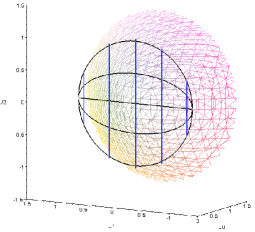
Figure 5: Projective plane for equidistant system is formed by equidistant and parallel straight lines

where $\tau_{1},\tau_{2}\in\mathbb{R}$ (see Fig. 5).

If we take $g(\xi,R)=-\xi/\alpha$, than nonorthogonal equidistant system has the form:

$$u_{0}=R\cosh\tau_{1}\cosh(\tau_{2}+R\tau_{1}/\alpha),\quad u_{1}=R\cosh\tau_{1}\sinh(\tau_{2}+R\tau_{1}/\alpha),\quad u_{2}=R\sinh\tau_{1}.$$ (58)

2b. On the one-sheeted hyperboloid ${\tilde{H}_{2}}$ function $f(\xi,R)$ can be positive or negative. When $f(\xi,R)>0$ ($|u_{2}|\geq R$) we have again $u_{0}=\sqrt{f(\xi,R})\cosh(\eta-g(\xi,R))$, but now $u_{2}=\pm\sqrt{f(\xi,R)+R^{2}}$.

Taking ${f(\xi,R})=R^{2}\sinh^{2}\xi$ and $g(\xi,R)=0$, renaming coordinates $(\xi,\eta)$ as $(\tau_{1},\tau_{2})$, we obtain the orthogonal equidistant coordinate system of type Ia that only covers part $|u_{2}|\geq R$ on ${\tilde{H}_{2}}$ (see Fig. 24):

$$u_{0}=R\sinh\tau_{1}\cosh\tau_{2},\quad u_{1}=R\sinh\tau_{1}\sinh\tau_{2},\quad u_{2}=\pm R\cosh\tau_{1},$$ (59)

where $\tau_{1},\tau_{2}\in\mathbb{R}$.

In the same manner, taking $g(\xi,R)=\ln[R\xi/\alpha]$ one can consider nonorthogonal $EQ$ system of Type Ia ($\tau_{1}\neq 0$):

$$u_{0}=R\sinh\tau_{1}\cosh\left(\tau_{2}-\ln[R\tau_{1}/\alpha]\right),\quad u_{1}=R\sinh\tau_{1}\sinh\left(\tau_{2}-\ln[R\tau_{1}/\alpha]\right),\quad u_{2}=\pm R\cosh\tau_{1}.$$ (60)

In case when $u_{0}^{2}-u_{1}^{2}\leq 0$ or $|u_{2}|\leq R$, the relations in formula (56) take the form

$$f(\xi,R)=u_{1}^{2}-u_{0}^{2}>0,\qquad\eta=\cosh^{-1}\frac{u_{1}}{\sqrt{f(\xi,R)}}+g(\xi,R).$$ (61)

By analogy with the previous case, but taking $f(\xi,R)=R^{2}\sin^{2}\xi$, we come to the equidistant coordinate system which covers part $|u_{2}|\leq R$ of one-sheeted hyperboloid ${\tilde{H}_{2}}$ (see Fig. 24):

$$u_{0}=R\sin\varphi\sinh\tau,\quad u_{1}=R\sin\varphi\cosh\tau,\quad u_{2}=R\cos\varphi,$$ (62)

where $\tau\in\mathbb{R}$, $\varphi\in[0,2\pi)$. We will call this system equidistant coordinates of type Ib. As for nonorthogonal $EQ$ system of type Ib, we take the same form $g(\xi,R)=\ln[R\xi/\alpha]$ and obtain ($\varphi\neq 0$):

$$u_{0}=R\sin\varphi\sinh\left(\tau-\ln[R\varphi/\alpha]\right),\quad u_{1}=R\sin\varphi\cosh\left(\tau-\ln[R\varphi/\alpha]\right),\quad u_{2}=R\cos\varphi.$$ (63)

Let us also note, that system (62) can be obtained from (59) through change: $\tau_{1}=-i\varphi$, $\tau_{2}=\tau+i\pi/2$. Moreover, the difference between systems of type Ia and Ib is manifested by the different contraction limits showed later.

Together with two equidistant coordinate systems of type Ia and Ib one can introduce the coordinate systems of IIa ($|u_{1}|\geqslant R$) and IIb ($|u_{1}|\leqslant R$) types, which diagonalize operator $S^{(1)}=K_{1}$. As a result we come to the same systems (59), (62) up to the permutation $u_{1}\leftrightarrow u_{2}$.

As for nonorthogonal equidistant coordinates IIb, we can consider, for example, the following ones:

$$u_{0}=-R\cos\varphi\sinh\left(\tau+R\varphi/\alpha\right),\quad u_{1}=R\sin\varphi,\quad u_{2}=-R\cos\varphi\cosh\left(\tau+R\varphi/\alpha\right).$$ (64)

3. ${S}^{(1)}=K_{1}+L$.

Let us consider operator $K_{1}+L=(u_{1}-u_{0})\partial_{u_{2}}-u_{2}\partial_{u_{0}}-u_{2}\partial_{u_{1}}$. To reduce it to canonical form $\partial_{\eta}$ we need to solve the following system

$$(u_{1}-u_{0})\frac{\partial\xi}{\partial u_{2}}-u_{2}\frac{\partial\xi}{\partial u_{0}}-u_{2}\frac{\partial\xi}{\partial u_{1}}=0,\qquad(u_{1}-u_{0})\frac{\partial\eta}{\partial u_{2}}-u_{2}\frac{\partial\eta}{\partial u_{0}}-u_{2}\frac{\partial\eta}{\partial u_{1}}=1.$$ (65)

Then,

$$f(\xi,R)=u_{0}-u_{1},\qquad u_{2}=g(\xi,R)-\eta f(\xi,R).$$ (66)

3a. For the case of two-sheeted hyperboloid (for the upper sheet) we have for orthogonal separable coordinates ($\xi,\eta)$ (we take $g=0$)

$$\xi=u_{0}-u_{1}>0,\qquad\eta=\frac{u_{2}}{u_{1}-u_{0}}.$$ (67)

Taking into account (1) with $\epsilon=1$ and putting $\eta=-\tilde{x}$, $\xi=R/\tilde{y}$ we obtain the orthogonal horicyclic system of coordinates (see Fig. 7):

$$u_{0}=R\frac{\tilde{x}^{2}+\tilde{y}^{2}+1}{2\tilde{y}},\quad u_{1}=R\frac{\tilde{x}^{2}+\tilde{y}^{2}-1}{2\tilde{y}},\quad u_{2}=R\frac{\tilde{x}}{\tilde{y}},$$ (68)

where $\tilde{x}\in\mathbb{R}$, $\tilde{y}>0$.

For nonorthogonal $HO$ system we take $f(\xi,R)=R/\xi$, $g(\xi,R)=R(1-1/\xi)$. Denoting $\xi=\tilde{y}$, $\eta=-\tilde{x}$ we have:

$$u_{0}=R\frac{\left(\tilde{x}+\tilde{y}-1\right)^{2}+\tilde{y}^{2}+1}{2\tilde{y}},\quad u_{1}=R\frac{\left(\tilde{x}+\tilde{y}-1\right)^{2}+\tilde{y}^{2}-1}{2\tilde{y}},\quad u_{2}=R\frac{\tilde{x}+\tilde{y}-1}{\tilde{y}}.$$ (69)

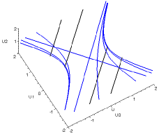
Figure 29: Projective plane for horicyclic system

3b. In the case of one-sheeted hyperboloid ($\epsilon=-1$) we get the following form of horicyclic system of coordinates (see Fig. 29):

$$u_{0}=R\frac{\tilde{x}^{2}-\tilde{y}^{2}+1}{2\tilde{y}},\qquad u_{1}=R\frac{\tilde{x}^{2}-\tilde{y}^{2}-1}{2\tilde{y}},\qquad u_{2}=R\frac{\tilde{x}}{\tilde{y}}.$$ (70)

where now $\tilde{x}\in\mathbb{R}$, $\tilde{y}\in\mathbb{R}\setminus\{0\}$.

Also we consider nonorthogonal $HO$ system of the form ($f(\xi,R)=R\xi/2$, $g(\xi,R)=R$):

$$u_{0}=\frac{R}{4}\left(\xi\eta^{2}-4\eta+\xi\right),\qquad u_{1}=\frac{R}{4}\left(\xi\eta^{2}-4\eta-\xi\right),\qquad u_{2}=R(1-\xi\eta/2).$$ (71)

It is clear that one can introduce the equivalent coordinate systems for (68), (70), (71) which diagonalize operator ${S}^{(1)}=K_{2}-L$ and are obtained by the permutation of coordinates $u_{1}$ and $u_{2}$.

2.2 Classification of second-order symmetries

Now let us consider the second-order operator $S^{(2)}$ from (9) of the enveloping algebra of $so(2,1)$:

$$S^{(2)}=aK_{1}^{2}+b\{K_{1},K_{2}\}+cK_{2}^{2}+d\{K_{1},L\}+e\{K_{2},L\}+fL^{2},$$ (72)

where $\{X,Y\}=XY+YX$.

The quadratic form

$$M=\left({{\begin{array}[]{*{20}c}a&b&d\\ b&c&e\\ d&e&f\end{array}}}\right)$$ (73)

corresponds to operator (72).

Under the automorphisms of group $A_{3}$ the elements of form $M$ are transformed as follows:

$${M}_{K_{1}}^{\prime}=A_{K_{1}}^{T}MA_{K_{1}}=$$ (74)

$$=\left({{\begin{array}[]{*{20}c}a&b\cosh a_{1}+d\sinh a_{1}&b\sinh a_{1}+d\cosh a_{1}\\ b\cosh a_{1}+d\sinh a_{1}&c\cosh^{2}a_{1}+e\sinh 2a_{1}+f\sinh^{2}a_{1}&(c+f)/2\sinh 2a_{1}+e\cosh 2a_{1}\\ b\sinh a_{1}+d\cosh a_{1}&(c+f)/2\sinh 2a_{1}+e\cosh 2a_{1}&c\sinh^{2}a_{1}+e\sinh 2a_{1}+f\cosh^{2}a_{1}\end{array}}}\right),$$ (78)

$${M}_{K_{2}}^{\prime}=A_{K_{2}}^{T}MA_{K_{2}},$$ (79)

$${M}_{L}^{\prime}=A_{L}^{T}MA_{L},$$ (80)

where $A^{T}$ means transposed matrix. So, we have two hyperbolic rotations (74), (79) and ordinary rotation (80).

We have to obtain the classification of matrices $M$ with respect to actions (74) – (80) and the linear combination with the Casimir operator ${\cal C}=K_{1}^{2}+K_{2}^{2}-L^{2}$:

$${M}_{\cal C}^{\prime}=\alpha_{1}M+\alpha_{2}\left({{\begin{array}[]{*{20}c}1&0&0\\ 0&1&0\\ 0&0&-1\end{array}}}\right)=\alpha_{1}M+\alpha_{2}A_{\cal C},$$ (81)

where $\alpha_{1}$ is non-zero constant.

The invariants of transformations (74) – (80) are the following ones:

$$I_{1}=a+c-f,\quad I_{2}=A+C-F,\quad I_{3}=\det M,$$

where $A$, $B$, $C$, …, $F$ are the minors of the elements $a$, $b$, $c$, …, $f$ of $M$ respectively.

In order to classify all $M$ forms let us consider the case when $I_{3}=0$. If it is not so, we can do it through transformation (81), namely ${M}_{\cal C}^{\prime}=M-\mu A_{\cal C}$, where $\mu$ is the real root of equation $\det(M-\mu A_{\cal C})=0$. If $\det M=0$, then there are the following relations for minors of $M$:

$$CF=E^{2},\qquad AF=D^{2},\qquad AC=B^{2},$$ (82)

and

$$aA-bB+dD=0,$$ (83)

$$-bB+cC-eE=0,$$ (84)

$$dD-eE+fF=0.$$ (85)

It is easy to see that transformations (74) – (80) act on the minors like on the elements of $M$, i.e. if we substitute $a$, $b$, $c$,… in (74) – (80) by the corresponding minors $A$, $B$, $C$,… we obtain the same transformations for minors.

Acting by rotation $A_{L}$ on minor $B$ it can be reduced to zero. Since $I_{3}$ is the invariant of group $A_{3}$, then relations (82) – (85) remain valid for the transformed minors. By virtue of (82) we have $AC=0$.

Case 1. If $A=0$, then $D=0$ due to (82). There are two cases to consider here.

1. $I_{2}\neq 0$, i.e. $C-F\neq 0$, then by suitable choice of parameter $a_{1}=\frac{1}{4}\ln\left(\frac{F+C-2E}{F+C+2E}\right)$, $E$ can be reduced to zero and minors $A$, $B$, $D$ stay equal to zero. Such value of the parameter exists because $(F+C-2E)(F+C+2E)=(C-F)^{2}>0$. Then from (82) we have $CF=0$. There are two possible cases:

   • $C=0,F\neq 0$, then $f=0$ from (85), so $e=0$ from $A=0$ and $d=0$ from $C=0$. Then we can vanish element $b$ by rotation $A_{L}$ Finally, we have

     $$M_{1}=\left.\left({{\begin{array}[]{*{20}c}a&0&0\\ 0&c&0\\ 0&0&0\end{array}}}\right)\right|_{F=ac\neq 0}.$$

   • $C\neq 0,F=0$, then $c=0$ from (84), so $e=0$ from $A=0$ and $b=0$ from $F=0$. Finally, we have

     $$M_{2}=\left.\left({{\begin{array}[]{*{20}c}a&0&d\\ 0&0&0\\ d&0&f\end{array}}}\right)\right|_{C=af-d^{2}\neq 0}.$$

2. $I_{2}=0$, i.e. $C=F$:

   • $C=F=0$, then $E=0$ from (82) that is all the minors are equal to zero and the automorphisms can not change any minor, but they can transform the elements of $M$. By appropriate choice of rotation $A_{L}$ element $b$ can be reduced to zero. If $a\neq 0$, then $c=0$ from $F=0$, $e=0$ from $E=0$ and we have form $M_{2}$ under the condition $C=0$. If $a=0$, then $d=0$ from $C=0$ and through rotation $A_{L}$ with $a_{3}=\pi/2$ we obtain the same form $M_{2}$.

   • $C=F\neq 0$, then $f=c$ from (84), (85), so $e=\pm c$ from $A=0$ and $d=\pm b$ from $C=F$. Using reflections one can reduce the form with the higher sign elements to the form with the lower sign elements and finally we have form

     $$M_{3}=\left.\left({{\begin{array}[]{*{20}c}a&b&-b\\ b&c&-c\\ -b&-c&c\end{array}}}\right)\right|_{ac\neq b^{2}}.$$

Case 2. If $A\neq 0$, then $C=0$ from (82), since $B=0$; and $E=0$ due to (82). There are two cases to consider here.

1. $I_{2}\neq 0$, i.e. $A-F\neq 0$, then by suitable choice of parameter $a_{2}=\frac{1}{4}\ln\left(\frac{A+F-2D}{A+F+2D}\right)$ minor $D$ can be reduced to zero and minors $C$, $B$, $E$ stay equal to zero. Such parameter $a_{2}$ exists, because $(A+F-2D)(A+F+2D)=(A-F)^{2}>0$. Then from (82) we have $AF=0$, so $F=0$. All minors except $A$ are equal to zero, so $a=0$ from (83). Then $d=0$ from $C=0$; $b=0$ from $F=0$. The obtained form can be reduced to form $M_{2}$ through rotation $A_{L}$ with $a_{3}=\pi/2$.

2. $I_{2}=A-F=0$, so $A=F\neq 0$. Then $f=a$ from (83), (84); so $d=\pm a$ from $C=0$ and $b=\pm e$ from $A=F$. Using reflections one can reduce the form with the higher sign elements to the form with the lower sign elements and finally we have form

   $$M_{4}=\left.\left({{\begin{array}[]{*{20}c}a&b&-a\\ b&c&-b\\ -a&-b&a\end{array}}}\right)\right|_{ac\neq b^{2}}.$$ (86)

Note, that

1. through rotation $A_{L}$ with parameter $a_{3}=\pi/2$ form $M_{3}$ is reduced to form $M_{4}$;

2. form $M_{1}$ through (81) with $\alpha_{1}=1/c$, $\alpha_{2}=-1$ is reduced to form $M_{2}$ with $a\neq-1$, $d=0$, $f=1$,

so there are two distinct inequivalent forms only: $M_{2}$ (without any condition) and $M_{4}$.

1. $M_{4}.$

If in (86) $I_{1}=c\neq 0$, then by the composition $A_{L}\circ A_{K_{1}}\circ A_{L}$ with parameters $\sin a_{3}=\sigma/\sqrt{\sigma^{2}+4}$, $\sinh a_{1}=-\sigma\sqrt{\sigma^{2}+4}/2$, $\sigma=-b/c$ we reduce it to form

$$\left.\left({{\begin{array}[]{*{20}c}a&0&-a\\ 0&c&0\\ -a&0&a\end{array}}}\right)\right|_{ac\neq 0},$$

then dividing it by $a$ and using reflections we obtain operators ($\gamma>0$):

$$S_{EP}=(K_{1}+L)^{2}+\gamma K_{2}^{2},\qquad\text{if}\quad ac>0,$$ (87)

$$S_{HP}=(K_{1}+L)^{2}-\gamma K_{2}^{2},\qquad\text{if}\quad ac<0.$$ (88)

If in (86) $I_{1}=c=0$, then $b\neq 0$, by the same composition $A_{L}\circ A_{K_{1}}\circ A_{L}$ with parameter $\sigma=-a/(2b)$ we make $a=0$, and after applying reflections and the division by $b$ we have operator

$$S_{SCP}=\{K_{1},K_{2}\}+\{K_{2},L\}.$$ (89)

2. $M_{2}.$
In this case the form looks like

$$M_{2}=\left({{\begin{array}[]{*{20}c}a&0&d\\ 0&0&0\\ d&0&f\end{array}}}\right)\cong\left({{\begin{array}[]{*{20}c}0&0&0\\ 0&c&e\\ 0&e&f\end{array}}}\right)=\widetilde{M}_{2}.$$ (90)

Here we need to consider the value of the invariant of transformation (79), namely $J=(a+f)^{2}-4d^{2}$ for $M_{2}$ (or the invariant for $A_{K_{1}}$: $\widetilde{J}=(c+f)^{2}-4e^{2}$ for $\widetilde{M}_{2}$).

1. $\widetilde{J}=(c+f)^{2}-4e^{2}>0$, then $c+f\neq 0$, and by the hyperbolic rotation (74) with $\tanh 2a_{1}=-2e/(c+f)$ we can vanish element $e$ in $\widetilde{M}_{2}$.

If $f=0$, then we have operator

$$S_{EQ}^{(2)}=K_{2}^{2}.$$ (91)

If $f\neq 0$, then dividing by $f$ we have form

$$\left.\left({{\begin{array}[]{*{20}c}0&0&0\\ 0&\overline{c}&0\\ 0&0&1\end{array}}}\right)\right|_{\widetilde{J}=(\overline{c}+1)^{2}>0,\>\overline{c}\neq-1}.$$ (92)

If $\overline{c}=0$ in (92), then we have operator

$$S_{SPH}^{(2)}=L^{2}.$$ (93)

If $\overline{c}\neq 0$, then from relation $\widetilde{J}=(\overline{c}+1)^{2}>0$ we have $\overline{c}\in(-\infty,-1)\cup(-1,0)\cup(0,\infty)$.

a. If $\overline{c}>0$ in (92), then putting $\overline{c}=\sinh^{2}\beta$, $\beta\neq 0$ we have operator

$$S_{E}=L^{2}+\sinh^{2}\beta K_{2}^{2},\qquad\beta\neq 0.$$ (94)

b. If $\overline{c}<-1$, then putting $\overline{c}^{2}=-1/\sin^{2}\alpha$, $\sin^{2}\alpha\neq 0,\neq 1$ and multiplying the operator by $-\sin^{2}\alpha$ we have operator

$$S_{H}=K_{2}^{2}-\sin^{2}\alpha\>L^{2},\quad\sin^{2}\alpha\neq 0,\neq 1.$$ (95)

c. Finally, for values $-1<\overline{c}<0$, we can take $\overline{c}=-\tanh^{2}\gamma$, $\gamma\neq 0$ and trough rotation (80) with $a_{3}=\pi/2$ we obtain

$$\left({{\begin{array}[]{*{20}c}-\tanh^{2}\gamma&0&0\\ 0&0&0\\ 0&0&1\end{array}}}\right).$$ (96)

Then, acting by (81) over (96) with $\alpha_{1}=\cosh^{2}\gamma$, $\alpha_{2}=\sinh^{2}\gamma$ we reduce the above form to the case of $S_{E}$ and there is no new operator.

Let us note, that applying hyperbolic rotation (79) with $a_{2}=\beta$ to the operator $S_{E}$ and using (81) with $\alpha_{1}=1$, $\alpha_{2}=\sinh^{2}\beta$ we obtain the rotated operator

$$S_{\tilde{E}}=\cosh 2\beta L^{2}+1/2\sinh 2\beta\{K_{1},L\},\qquad\beta\neq 0.$$ (97)

2. $J=0$, so $(a+f)^{2}=4d^{2}$, $d\neq 0$ (if $d=0$, then $a=-f$ and we have operator $S_{H}$ with $\sin^{2}\alpha=1$, but in this case $S_{H}-\Delta=K_{2}^{2}-L^{2}-(K_{1}^{2}+K_{2}^{2}-L^{2})=-K_{1}^{2}\sim K_{2}^{2}=S_{EQ}$). So $|a+f|=2|d|$, or dividing it by $d$: $|a+f|=2$.

a. If $I_{1}=0$, i.e. $a=f$ and $a=f=\pm 1$, using reflections we obtain

$$S_{HO}^{(2)}=(K_{1}+L)^{2}.$$ (98)

b. If $I_{1}\neq 0$, i.e. $a\neq f$, and we can take $f=2-a$, if it’s not so, then trough reflections we can do it, so we have

$$\left.\left({{\begin{array}[]{*{20}c}a&0&1\\ 0&0&0\\ 1&0&2-a\end{array}}}\right)\right|_{a\neq 1}.$$ (99)

Then using (81) with $\alpha_{2}=1-a$, $\alpha_{1}=1$ we can reduce the form (99) to

$$\left({{\begin{array}[]{*{20}c}1&0&1\\ 0&\gamma&0\\ 1&0&1\end{array}}}\right),$$ (100)

where $\gamma=1-a\neq 0$ that corresponds to operator $\gamma K^{2}_{2}+(K_{1}+L)^{2},$ and it is equivalent to the form $M_{4}$ with $b=0$.

3. $J=(a+f)^{2}-4d^{2}<0$, $d\neq 0$, then by (79) we can obtain $a=-f$, so by (81) with $\alpha_{1}=1/d$, $\alpha_{2}=-a/d$ we have

$$\left({{\begin{array}[]{*{20}c}0&0&1\\ 0&c&0\\ 1&0&0\end{array}}}\right),$$

that corresponds to operator $S_{SH}$, if we put $c=\sinh 2\beta$:

$$S_{SH}=\sinh 2\beta K_{2}^{2}+\{K_{1},L\}.$$ (101)

Thus, we have obtained nine second order operators $S^{(2)}_{\alpha}$ of the enveloping algebra of $so(2,1)$. Each of them presents nonequivalent class with respect to the group of inner automorphisms $A_{3}$.

2.3 Second-order symmetries and non-subgroup coordinates on two-dimensional hyperboloids

Here we briefly describe the method of simultaneous diagonalization of the two second order operators $\Delta_{LB}$ and $S^{(2)}_{\alpha}$ (see also [67]). We will use the analogy with classical mechanics which simplifies our discussion. As it is known on the space of constant curvature the Schroedinger and Hamilton-Jacobi equation separates in the same systems of coordinates.

Let us take some local coordinate system $\xi=(\xi^{1},\xi^{2})$ that defines metric tensor (6) in space (1). For that system the classic Hamiltonian, describing a free motion, takes the form

$${\cal H}(\xi,p)=g^{ik}p_{i}p_{k},\qquad i,k=1,2,$$ (102)

where $p_{i}$ are the momenta classically conjugated to coordinates $\xi^{i}$. Let there exist the quadratic integral of motion ${\cal S}(\xi,p)$ which is in involution with Hamiltonian (102)

$${\cal S}(\xi,p)=a^{ik}(\xi)p_{i}p_{k},\qquad a^{ik}=a^{ki},$$ (103)

where tensor $a^{ik}$ is called Killing tensor of the second rank. Analogically, we can consider for the same space the motion of a free particle in quantum mechanics which is described simultaneously by two commuting operators, that is, by Hamiltonian and by quadratic integral of motion:

$$H=\Delta_{LB}=\frac{1}{\sqrt{g}}\,\frac{\partial}{\partial\xi^{i}}\sqrt{g}\,g^{ik}\,\frac{\partial}{\partial\xi^{k}},\qquad\qquad S=\frac{1}{\sqrt{g}}\,\frac{\partial}{\partial\xi^{i}}\sqrt{g}\,a^{ik}\,\frac{\partial}{\partial\xi^{k}},\qquad i,k=1,2.$$ (104)

The task is to find orthogonal coordinates $(\lambda_{1},\lambda_{2})$ which admit in classic mechanics the additive separation of variables related to equations ${\cal H}(\xi,p)=\mathcal{E}$ and ${\cal S}(\xi,p)=\mu$. In the case of quantum mechanics there is a multiplicative separation of variables related to the system of equations: $H\Psi=\mathcal{E}\Psi$ and $S\Psi=\mu\Psi$ where $\mu$ is a separation constant.

Such a coordinate system, generally speaking, can be determined from the condition of simultaneous reduction of quadratic forms ${\cal H}$ and ${\cal S}$ to canonic ones when matrices $g^{ik}$ and $a^{ik}$ are of diagonal type. To make it, according to the general theory, one needs to solve equation

$$\det(a^{ik}-\lambda g^{ik})=0.$$ (105)

Let us note that if one of the quadratic form, for example ${\cal H}(\xi,p)$ has the positive-definite associated matrix, then due to well known theorem from algebra, both roots $\lambda_{1}$ and $\lambda_{2}$ are real and distinct throughout space (1). Moreover, form ${\cal H}(\xi,p)$ is reduced to the normal form (all coefficients of quadratic form are equal to unit), but form ${\cal S}(\xi,p)$ is diagonalized (is of canonic form, see [47], p. 219). In such a way it is possible to choose some new orthogonal coordinates as a functions of the roots $\lambda_{1}$ and $\lambda_{2}$: $u(\lambda_{1})$ and $v(\lambda_{2})$ for which ${\cal H}$ and ${\cal S}$ simultaneously take the following form:

$${\cal H}=\frac{1}{\alpha(u)+\beta(v)}\left(p_{u}^{2}+p_{v}^{2}\right)=\mathcal{E},\qquad\qquad{\cal S}=\frac{1}{\alpha(u)+\beta(v)}\left(\alpha(u)p_{u}^{2}-\beta(v)p_{v}^{2}\right)=\mu.$$ (106)

The form of Hamiltonian ${\cal H}$ in (106) is called the Liouville form [66]. Finally, the procedure of separation of variables for Hamilton-Jacobi equation leads to two equations:

$$\beta{\cal H}+{\cal S}=\beta\mathcal{E}+\mu,\qquad\qquad\alpha{\cal H}-{\cal S}=\alpha\mathcal{E}-\mu.$$ (107)

By the analogy, for Helmholtz equation we have

$$(\beta{H}+{S})\Psi=(\beta\mathcal{E}+\mu)\Psi,\qquad\qquad(\alpha{H}-{S})\Psi=(\alpha\mathcal{E}-\mu)\Psi.$$ (108)

If none of quadratic forms is positive definite, then condition (105) does not guarantee the existence of the real or distinct eigenvalues. It may happen that $\lambda_{1}=\lambda_{2}$ or $\lambda_{1}$ and $\lambda_{2}$ are real ones only in some part of space and they do not provide the parametrization of whole hyperboloid (1). We can see this situation for the construction of coordinate system on one-sheeted hyperboloid.

Now let us write down the direct algorithm to obtain the separable coordinate system corresponding to the one of symmetry forms determined in subsection 2.2.

Let us take pseudo-spherical coordinates $(\tau,\varphi)$ (49) as local ones $\xi=(\xi^{1},\xi^{2})$ on two-sheeted hyperboloid. Components $g_{ik}$ for this coordinate system are as follows:

$$g_{ik}=R^{2}\mathop{\mathrm{diag}}(1,\sinh^{2}\tau),\qquad g^{ik}=R^{-2}\mathop{\mathrm{diag}}(1,1/\sinh^{2}\tau),\qquad\sinh^{2}\tau=R^{-2}(u_{1}^{2}+u_{2}^{2}).$$ (109)

The classical free Hamiltonian (102) is

$${\cal H}=g^{ik}p_{i}p_{k}=\frac{1}{R^{2}}\left(p_{\tau}^{2}+\frac{1}{\sinh^{2}\tau}p_{\varphi}^{2}\right)=\frac{1}{R^{2}}\left(p_{\tau}^{2}+\frac{R^{2}}{u_{1}^{2}+u_{2}^{2}}p_{\varphi}^{2}\right),$$ (110)

and the symmetry elements $K_{1}$, $K_{2}$, $L$ have the form (in ambient space coordinates)

$$K_{1}=-\frac{u_{2}}{\sqrt{u_{1}^{2}+u_{2}^{2}}}p_{\tau}-\frac{u_{0}u_{1}}{u_{1}^{2}+u_{2}^{2}}p_{\varphi},\qquad K_{2}=-\frac{u_{1}}{\sqrt{u_{1}^{2}+u_{2}^{2}}}p_{\tau}+\frac{u_{0}u_{2}}{u_{1}^{2}+u_{2}^{2}}p_{\varphi},\qquad L=p_{\varphi},$$ (111)

where $p_{\tau}$, $p_{\varphi}$ are classically conjugated to coordinates $(\tau,\varphi)$.

In the case of one-sheeted hyperboloid $u_{0}^{2}-u_{1}^{2}-u_{2}^{2}=-R^{2}$ we use pseudo-spherical coordinates defined by (51). The components of metric tensor are as follows:

$$g_{ik}=R^{2}\mathop{\mathrm{diag}}(1,-\cosh^{2}\tau),\qquad g^{ik}=R^{-2}\mathop{\mathrm{diag}}(1,-1/\cosh^{2}\tau).$$ (112)

Formulas (111) for operators $K_{1}$, $K_{2}$, $L$ are the same, but for classic Hamiltonian (102) we obtain

$${\cal H}=g^{ik}p_{i}p_{k}=\frac{1}{R^{2}}\left(p_{\tau}^{2}-\frac{1}{\cosh^{2}\tau}p_{\varphi}^{2}\right)=\frac{1}{R^{2}}\left(p_{\tau}^{2}-\frac{R^{2}}{u_{1}^{2}+u_{2}^{2}}p_{\varphi}^{2}\right).$$ (113)

Using relations (111), we write down the polynomial $S^{(2)}_{\alpha}$ in the quadratic form

$$S^{(2)}_{\alpha}=Ap_{\tau}^{2}+2Bp_{\tau}p_{\varphi}+Cp_{\varphi}^{2},$$ (114)

where in general the coefficients $A$, $B$, $C$ are the functions of the variables ($\tau,\varphi$) or ambient space variables ($u_{0},u_{1},u_{2})$. Later we will work in the ambient coordinate system ($u_{0},u_{1},u_{2}$) as a more universal one.

We need to diagonalize the matrix corresponding to form (114) by finding the eigenvalues from equation (105)

$$\det(a^{ik}-\lambda g^{ik})=\left|{{\begin{array}[]{*{20}c}A-\frac{\lambda}{g_{11}}&B\\ B&C-\frac{\lambda}{g_{22}}\end{array}}}\right|=0,$$ (115)

which corresponds to the system of two algebraic equations

$$\lambda_{1}+\lambda_{2}=Ag_{11}+Cg_{22},\quad\lambda_{1}\lambda_{2}=(AC-B^{2})g_{11}g_{22}$$ (116)

and admits two different and real roots if the following condition is satisfied

$$(Ag_{11}-Cg_{22})^{2}+4B^{2}g_{11}g_{22}>0.$$ (117)

Resolving above system (116) with the relation $u_{0}^{2}-u_{1}^{2}-u_{2}^{2}=\epsilon R^{2}$, $\epsilon=\pm 1$ we can determine separable orthogonal systems of coordinates on two- or one-sheeted hyperboloids. Let us note that in the case of two-sheeted hyperboloid we have $g_{11}g_{22}>0$ and inequality (117) is satisfied automatically. Thus, two different and real roots $\lambda_{1}$ and $\lambda_{2}$ exist. The corresponding problem on one-sheeted hyperboloid is more complicated. It may happen that $\lambda_{1}$ and $\lambda_{2}$ are real only on a part of ${\tilde{H}}_{2}$ hyperboloid and, therefore, do not parametrize the whole space.

We conserved the names given in article [85] for every operator $S^{(2)}_{\alpha}$: Equidistant coordinates $S_{EQ}=K_{2}^{2}$, Spherical coordinates $S_{SPH}=L^{2}$, Horiciclic coordinates $S_{HO}=(K_{1}+L)^{2}$, Semi-circular-parabolic coordinates $S_{SCP}$, Elliptic-parabolic coordinates $S_{EP}$, Hyperbolic-parabolic coordinates $S_{HP}$, Elliptic coordinates $S_{E}$ ($S_{\tilde{E}}$ for rotated elliptic coordinates), Hyperbolic coordinates $S_{H}$ and $S_{SH}$ for Semi-hyperbolic coordinates. Three first operators, namely: $S_{EQ}$, $S_{SPH}$ and $S_{HO}$ are the squares of the first order operators and provide the separation of variables in subgroup coordinate systems. Other six operators are non-subgroup ones.

Five operators: $S_{EP}$, $S_{HP}$, $S_{E}$, ($S_{\tilde{E}}$), $S_{H}$ and $S_{SH}$ depend on one dimensionless parameter, let us call it $\gamma$. The limit $\gamma\to 0$ (or $\gamma\to\infty$) simplifies significantly operators $S^{(2)}_{\alpha}$ and corresponding coordinates degenerate into a simpler subgroup systems (except the system for $S_{SCP}$).

2.4 Semi-hyperbolic system of coordinates

1.   Firstly let us consider two-sheeted hyperboloid. Writing down the operator $S_{SH}=\sinh 2\beta K_{2}^{2}+\{K_{1},L\}$ as in equation (114) and using formula (109) we get that the algebraic system (116) takes the form

$$\lambda_{1}+\lambda_{2}=2u_{0}u_{1}+c(u_{1}^{2}-u_{0}^{2}),\qquad\lambda_{1}\lambda_{2}=-R^{2}(u_{2}^{2}+2cu_{0}u_{1})$$ (118)

with $c=\sinh 2\beta$. Solution of (118) provides the algebraic form of semi-hyperbolic system of coordinates in terms of independent variables $\lambda_{1}$, $\lambda_{2}$:

$$u_{0}^{2} = \frac{R^{2}}{2(c^{2}+1)}\left\{\sqrt{(c^{2}+1)\left(1+\frac{\lambda_{1}^{2}}{R^{4}}\right)\left(1+\frac{\lambda_{2}^{2}}{R^{4}}\right)}+1-\frac{\lambda_{1}}{R^{2}}\frac{\lambda_{2}}{R^{2}}-c\left(\frac{\lambda_{1}}{R^{2}}+\frac{\lambda_{2}}{R^{2}}\right)\right\},$$

$$u_{1}^{2} = \frac{R^{2}}{2(c^{2}+1)}\left\{\sqrt{(c^{2}+1)\left(1+\frac{\lambda_{1}^{2}}{R^{4}}\right)\left(1+\frac{\lambda_{2}^{2}}{R^{4}}\right)}-1+\frac{\lambda_{1}}{R^{2}}\frac{\lambda_{2}}{R^{2}}+c\left(\frac{\lambda_{1}}{R^{2}}+\frac{\lambda_{2}}{R^{2}}\right)\right\},$$ (119)

$$u_{2}^{2} = -\frac{R^{2}}{c^{2}+1}\left(\frac{\lambda_{1}}{R^{2}}+c\right)\left(\frac{\lambda_{2}}{R^{2}}+c\right).$$

where we choose that $\lambda_{2}/R^{2}<-c<\lambda_{1}/R^{2}$. It is clear from (2.4) for $SH$ coordinate system that the relation between ($\lambda_{1},\lambda_{2}$) and Cartesian coordinates ($u_{0},u_{1},u_{2}$) is not ”one-to-one”. For every value of $\lambda_{1}$, $\lambda_{2}$ there are eight corresponding points ($\pm u_{0},\pm u_{1},\pm u_{2}$) in ambient space $E_{2,1}$.

Geometrically the semi-hyperbolic system (2.4) consists of two families of confocal semi-hyperbolas. The distance between the semi-hyperbolas focus and the basis of its equidistances is equal to $2\beta R$. The dimensionless parameter $c=\sinh 2\beta$ defines the position of the semi-hyperbolas focus on the upper sheet of two-sheeted hyperboloid (Fig. 15). One can obtain its coordinates making $\lambda_{1}/R^{2}\to-c$ and $\lambda_{2}/R^{2}\to-c$, then $F\left(u_{0},u_{1},u_{2}\right)\equiv F\left(R\frac{\sqrt{\sqrt{c^{2}+1}+1}}{\sqrt{2}},\right.$ $\left.-R\frac{\sqrt{\sqrt{c^{2}+1}-1}}{\sqrt{2}},\,0\right)$.

There exist two simple particular cases of $SH$ system, namely: $c=0$ and $c=1$. For the first case the focus coordinates are $F\left(R,0,0\right)$ and symmetry operator takes the simple form $S_{SH}=\{K_{1},L\}$. Then system (2.4) can be rewritten in new coordinates $\lambda_{1}/R^{2}=\mu_{1}$ and $\lambda_{2}/R^{2}=-\mu_{2}$:

$$u_{0}^{2} = \frac{R^{2}}{2}\left\{\sqrt{(1+\mu_{1}^{2})(1+\mu_{2}^{2})}+\mu_{1}\mu_{2}+1\right\},$$

$$u_{1}^{2} = \frac{R^{2}}{2}\left\{\sqrt{(1+\mu_{1}^{2})(1+\mu_{2}^{2})}-\mu_{1}\mu_{2}-1\right\},$$ (120)

$$u_{2}^{2} = R^{2}\mu_{1}\mu_{2},$$

where $\mu_{1},\mu_{2}\geq 0$. For the second case $c=1$ we have $S_{SH}=K_{2}^{2}+\{K_{1},L\}$. Introducing dimensionless variables $\lambda_{1}/R^{2}=\sinh\tau_{1}$ and $\lambda_{2}/R^{2}=\sinh\tau_{2}$ ($\sinh\tau_{2}<-1<\sinh\tau_{1}$) we get the trigonometric form of semi-hyperbolic coordinate system

$$u_{0}^{2} = \frac{R^{2}}{4}\left[\sqrt{2}\cosh\tau_{1}\cosh\tau_{2}-(\sinh\tau_{1}+1)(\sinh\tau_{2}+1)+2\right],$$

$$u_{1}^{2} = \frac{R^{2}}{4}\left[\sqrt{2}\cosh\tau_{1}\cosh\tau_{2}+(\sinh\tau_{1}+1)(\sinh\tau_{2}+1)-2\right],$$ (121)

$$u_{2}^{2} = -\frac{R^{2}}{2}(\sinh\tau_{1}+1)(\sinh\tau_{2}+1).$$

For the large values of parameter $c\to\infty$ ($\beta\to\infty$) the focus goes to infinity and $SH$ system degenerates to the equidistant one. For the operator we have $S_{SH}/\sinh 2\beta=K_{2}^{2}+\{K_{1},L\}/\sinh 2\beta\to K_{2}^{2}$. Indeed, as $\beta\to\infty$ one can make that the variable $\lambda_{2}$ tends to $-\infty$ and at the same time the domain of $\lambda_{1}$ is expanded: $\lambda_{1}\in(-\infty,\infty)$. Putting $-\lambda_{2}/\sinh 2\beta=R^{2}\cosh^{2}\tau_{1}$, $\lambda_{1}=R^{2}\sinh 2\tau_{2}$ in (2.4) and taking $\beta\to\infty$ we come to equidistant system in form (57).

Finally, note that putting $c=\frac{a-\gamma}{\delta}$, where $\alpha,\delta,\gamma$ are some constants and introducing new variables accordingly to the relations $\lambda_{1}=R^{2}\left(\frac{a-\rho_{1}}{\delta}-c\right)$ and $\lambda_{2}=R^{2}\left(\frac{a-\rho_{2}}{\delta}-c\right)$, semi-hyperbolic system of coordinates (2.4) takes the well known form (see [61, 85]).

2.   In the case of one-sheeted hyperboloid instead of the algebraic equations (118) we have the following system

$$\lambda_{1}+\lambda_{2}=2u_{0}u_{1}+c(u_{1}^{2}-u_{0}^{2}),\qquad\lambda_{1}\lambda_{2}=R^{2}(u_{2}^{2}+2cu_{0}u_{1}).$$ (122)

Indeed equations (118) and (122) are connected by the transformation $R\to iR$. Therefore the roots $\lambda_{1}$, $\lambda_{2}$ are real and distinct when inequality (117) is satisfied

$$|2u_{0}u_{1}+c(u_{1}^{2}-u_{0}^{2})|>2R\sqrt{u_{2}^{2}+2cu_{0}u_{1}}$$ (123)

and are complex otherwise. Using now the substitutions $\lambda_{1}/R^{2}=\sinh\tau_{1}$ and $\lambda_{2}/R^{2}=\sinh\tau_{2}$ we get the analog of trigonometric form of semi-hyperbolic coordinates (see Fig. 38):

$$u_{0}^{2} = \frac{R^{2}}{2(c^{2}+1)}\left\{\sqrt{c^{2}+1}\cosh\tau_{1}\cosh\tau_{2}+(\sinh\tau_{1}-c)(\sinh\tau_{2}-c)-c^{2}-1\right\},$$

$$u_{1}^{2} = \frac{R^{2}}{2(c^{2}+1)}\left\{\sqrt{c^{2}+1}\cosh\tau_{1}\cosh\tau_{2}-(\sinh\tau_{1}-c)(\sinh\tau_{2}-c)+c^{2}+1\right\},$$ (124)

$$u_{2}^{2} = \frac{R^{2}}{c^{2}+1}(\sinh\tau_{1}-c)(\sinh\tau_{2}-c),$$

where $\sinh\tau_{1},\sinh\tau_{2}\leq c$ ($SH$ of Type I) or $\sinh\tau_{1},\sinh\tau_{2}\geq c$ ($SH$ of Type II). The above coordinate grid has two pairs of envelopes defined by equality $|2u_{0}u_{1}+c(u_{1}^{2}-u_{0}^{2})|=2R\sqrt{u_{2}^{2}+2cu_{0}u_{1}}$. The points of its intersections have coordinates $\left(\pm R\frac{\sqrt{\sqrt{c^{2}+1}-1}}{\sqrt{2}},\right.$ $\left.\mp R\frac{\sqrt{\sqrt{c^{2}+1}+1}}{\sqrt{2}},\,0\right)$. It is necessary to adjust the intervals for coordinate lines $\tau_{i}=\text{const}$. For example, one can take points of envelops as initial ones for family $\tau_{1}=\text{const.}$ and as endpoints for the other family $\tau_{2}=\text{const.}$

Let us note that coordinate system (2.4) can be constructed from (2.4) by the transformations $R\to iR$, $\tau_{1}\to\tau_{1}-i\pi$ and $\tau_{2}\to-\tau_{2}$.

In case of $c=0$ the inequality (123) is equivalent to $|u_{1}|\geq R$. The change of variable $\mu_{1}=\sinh\tau_{1}$, $\mu_{2}=\sinh\tau_{2}$ leads to the following parametrization of coordinates:

$$u_{0}^{2} = \frac{R^{2}}{2}\left\{\sqrt{(1+\mu_{1}^{2})(1+\mu_{2}^{2})}+\mu_{1}\mu_{2}-1\right\},$$

$$u_{1}^{2} = \frac{R^{2}}{2}\left\{\sqrt{(1+\mu_{1}^{2})(1+\mu_{2}^{2})}-\mu_{1}\mu_{2}+1\right\},$$ (125)

$$u_{2}^{2} = R^{2}\mu_{1}\mu_{2},$$

where $\mu_{1},\mu_{2}\geq 0$.

2.5 Semi-circular-parabolic system of coordinates

1.   System (116) for $S_{SCP}=\{K_{1},K_{2}\}+\{K_{2},L\}$ on two-sheeted hyperboloid has the form

$$\lambda_{1}+\lambda_{2}=2u_{2}(u_{1}-u_{0}),\qquad\lambda_{1}\lambda_{2}=-R^{2}(u_{1}-u_{0})^{2}.$$ (126)

Resolving system (126), and making the change of variables $\lambda_{1}=-R^{2}/\xi^{2}$, $\lambda_{2}=R^{2}/\eta^{2}$ we obtain the semi-circular-parabolic coordinate system (Fig. 21):

$$u_{0}=R\frac{\left(\eta^{2}+\xi^{2}\right)^{2}+4}{8\xi\eta},\quad u_{1}=R\frac{\left(\eta^{2}+\xi^{2}\right)^{2}-4}{8\xi\eta},\quad u_{2}=R{\frac{{\eta}^{2}-{\xi}^{2}}{2\xi\eta}},$$ (127)

where $\xi$, $\eta>0$.

2.   In case of the one-sheeted hyperboloid we have

$$\lambda_{1}+\lambda_{2}=2u_{2}(u_{1}-u_{0}),\qquad\lambda_{1}\lambda_{2}=R^{2}(u_{1}-u_{0})^{2}.$$ (128)

In this case coordinate system covers only the part of hyperboloid when $|u_{2}|>R$ (Fig. 46) and has the following form

$$u_{0}=R\frac{\left(\eta^{2}-\xi^{2}\right)^{2}+4}{8\xi\eta},\quad u_{1}=R\frac{\left(\eta^{2}-\xi^{2}\right)^{2}-4}{8\xi\eta},\quad u_{2}=\pm R{\frac{{\eta}^{2}+{\xi}^{2}}{2\xi\eta}},$$ (129)

where we introduce new variables $\lambda_{1}=R^{2}/\xi^{2}$, $\lambda_{2}=R^{2}/\eta^{2}$ and $\xi>0$ , $\eta\in\mathbb{R}\setminus\{0\}$. Sign $\pm$ for $u_{2}$ corresponds to the case $\lambda_{1},\lambda_{2}<0$. Let us note that lines $u_{0}\pm u_{1}=0$, $|u_{2}|=R$ are envelopes for families of coordinate lines $\xi=\text{const.}$ (or $\eta=\text{const.}$). To distinguish coordinate lines one needs to select the appropriate intervals. Thus, points of envelopes can be taken as initial ones. For example, for the fixed line $\xi=\xi_{0}$ the interval for $\eta$ is $(-\infty,-\xi_{0})\cup(\xi_{0},+\infty)$.

2.6 Elliptic-parabolic system of coordinates

1. Let us consider the operator $S_{EP}=\gamma K_{2}^{2}+\left(K_{1}+L\right)^{2}$, $\gamma>0$. For such operator, system (116) takes the form

$$\lambda_{1}+\lambda_{2}=(u_{0}-u_{1})^{2}+\gamma(u_{0}^{2}-u_{1}^{2}),\qquad\lambda_{1}\lambda_{2}=\gamma R^{2}(u_{0}-u_{1})^{2},$$ (130)

where we have preliminary changed the signs of $\lambda_{i}$: $\lambda_{i}\to-\lambda_{i}$. Let us take the solution of system (130) as follows

$$u_{0} = \frac{1}{2\sqrt{\gamma^{3}\lambda_{1}\lambda_{2}}}\left(\frac{\gamma-1}{R}\lambda_{1}\lambda_{2}+\gamma R(\lambda_{1}+\lambda_{2})\right),$$

$$u_{1} = \frac{1}{2\sqrt{\gamma^{3}\lambda_{1}\lambda_{2}}}\left(-\frac{\gamma+1}{R}\lambda_{1}\lambda_{2}+\gamma R(\lambda_{1}+\lambda_{2})\right),$$ (131)

$$u_{2}^{2} = \frac{R^{2}}{\gamma^{2}}\left(\frac{\lambda_{1}}{R^{2}}-\gamma\right)\left(\gamma-\frac{\lambda_{2}}{R^{2}}\right),$$

where $0<\lambda_{2}/R^{2}\leq\gamma\leq\lambda_{1}/R^{2}$. If we choose $\lambda_{1}=R^{2}\gamma/\cos^{2}\theta$ and $\lambda_{2}=R^{2}\gamma/\cosh^{2}a$, we obtain the elliptic-parabolic system of coordinates in the trigonometric form (Fig. 17)

$$u_{0}=\frac{R}{\sqrt{\gamma}}\frac{\cosh^{2}a-\sin^{2}\theta+\gamma}{2\cos\theta\cosh a},\quad u_{1}=\frac{R}{\sqrt{\gamma}}\frac{\cosh^{2}a-\sin^{2}\theta-\gamma}{2\cos\theta\cosh a},\quad u_{2}=R\tan\theta\tanh a,$$ (132)

where $a\geq 0$, $\theta\in\left(-\frac{\pi}{2},\frac{\pi}{2}\right)$. Geometrically positive parameter $\gamma$ defines the position of the focus of elliptic parabolas lying on hyperboloid $H_{2}$. One can get its coordinates in limits $\cos\theta\to 1$, $\cosh a\to 1$. Thus we have

$$F\left(u_{0},u_{1},u_{2}\right)\equiv F\left(R\frac{\gamma+1}{2\sqrt{\gamma}},\,R\frac{\gamma-1}{2\sqrt{\gamma}},\,0\right).$$ (133)

2. For one-sheeted hyperboloid we obtain

$$\lambda_{1}+\lambda_{2}=(u_{0}-u_{1})^{2}+\gamma(u_{0}^{2}-u_{1}^{2}),\qquad\lambda_{1}\lambda_{2}=-\gamma R^{2}(u_{0}-u_{1})^{2}$$ (134)

and the corresponding system of coordinates takes the form (see Fig. 40)

$$u_{0} = \pm\frac{1}{2\sqrt{-\gamma^{3}\lambda_{1}\lambda_{2}}}\left(\frac{1-\gamma}{R}\lambda_{1}\lambda_{2}+\gamma R(\lambda_{1}+\lambda_{2})\right),$$

$$u_{1} = \pm\frac{1}{2\sqrt{-\gamma^{3}\lambda_{1}\lambda_{2}}}\left(\frac{1+\gamma}{R}\lambda_{1}\lambda_{2}+\gamma R(\lambda_{1}+\lambda_{2})\right),$$ (135)

$$u_{2}^{2} = \frac{R^{2}}{\gamma^{2}}\left(\frac{\lambda_{1}}{R^{2}}+\gamma\right)\left(\frac{\lambda_{2}}{R^{2}}+\gamma\right),$$

where $-\gamma\leq\lambda_{2}/R^{2}<0<\lambda_{1}/R^{2}$ (or $-\gamma\leq\lambda_{1}/R^{2}<0<\lambda_{2}/R^{2}$). Putting $\lambda_{2}/(R^{2}\gamma)=-1/\cosh^{2}\tau_{1}$ and $\lambda_{1}/(R^{2}\gamma)=1/\sinh^{2}\tau_{2}$ we can rewrite the elliptic-parabolic system of coordinates on ${\tilde{H}}_{2}$ hyperboloid in form

$$u_{0}=\frac{R}{\sqrt{\gamma}}\frac{\cosh^{2}\tau_{1}-\cosh^{2}\tau_{2}+\gamma}{2\cosh\tau_{1}\sinh\tau_{2}},\quad u_{1}=\frac{R}{\sqrt{\gamma}}\frac{\cosh^{2}\tau_{1}-\cosh^{2}\tau_{2}-\gamma}{2\cosh\tau_{1}\sinh\tau_{2}},\quad u_{2}=R\tanh\tau_{1}\coth\tau_{2},$$ (136)

where now $\tau_{1}\in\mathbb{R}$, $\tau_{2}\in\mathbb{R}\setminus\{0\}$. Let us note that on ${\tilde{H}}_{2}$ parameter $\gamma$ can be considered as a scale factor.

The elliptic-parabolic system as the one-parametric one includes two simple limiting cases, namely, the small and the large values of parameter $\gamma$, when the coordinates of focus (133) on $H_{2}$ move to the infinity. For $\gamma\sim 0$ we get that $S_{EP}\sim\left(K_{1}+L\right)^{2}$, whereas, for large $\gamma$: $S_{EP}/\gamma\sim K_{2}^{2}$ and therefore $S_{EP}$ coordinates degenerate to the horicyclic and equidistant system correspondingly. Thus, from equation (130) we have

$$\lambda_{1,2}=\frac{(u_{0}-u_{1})^{2}}{2}\left[1+\gamma\frac{u_{0}+u_{1}}{u_{0}-u_{1}}\pm\sqrt{1+2\gamma\frac{u_{2}^{2}-R^{2}}{(u_{0}-u_{1})^{2}}+\gamma^{2}\frac{(u_{0}+u_{1})^{2}}{(u_{0}-u_{1})^{2}}}\right],$$ (137)

we get for $\gamma\sim 0$: $\cosh a\sim 1+\gamma{\tilde{x}}^{2}/2$, $\cos\theta\sim\sqrt{\gamma}{\tilde{y}}$ and for large $\gamma\sim\infty$: $\cosh a\sim\sqrt{\gamma}e^{\tau_{2}}$, $\sin\theta\sim\tanh\tau_{1}$. Putting these results into equation (132) it is easy to obtain the limiting horicylic (68) and equidistant (57) systems of coordinates respectively. By analogy one can prove that the elliptic-parabolic coordinates on one-sheeted hyperboloid degenerate to the same ones.

It is also important to note that elliptic-parabolic coordinates introduced in (132) and (136) cover the two- and one-sheeted hyperboloids completely.

2.7 Hyperbolic-parabolic system of coordinates

1. Let us consider operator $S_{HP}=-\gamma K_{2}^{2}+\left(K_{1}+L\right)^{2}$, $\gamma>0$. In this case we obtain (up to the change of sign $\gamma\to-\gamma$) the same algebraic equations as in (130). The solution looks as follows

$$u_{0} = \frac{-1}{2\sqrt{-\gamma^{3}\lambda_{1}\lambda_{2}}}\left(\frac{1+\gamma}{R}\lambda_{1}\lambda_{2}+\gamma R(\lambda_{1}+\lambda_{2})\right),$$

$$u_{1} = \frac{-1}{2\sqrt{-\gamma^{3}\lambda_{1}\lambda_{2}}}\left(\frac{1-\gamma}{R}\lambda_{1}\lambda_{2}+\gamma R(\lambda_{1}+\lambda_{2})\right),$$ (138)

$$u_{2}^{2} = -\frac{R^{2}}{\gamma^{2}}\left(\frac{\lambda_{1}}{R^{2}}+\gamma\right)\left(\frac{\lambda_{2}}{R^{2}}+\gamma\right),$$

where $\lambda_{2}/R^{2}\leq-\gamma<0<\lambda_{1}/R^{2}$. If we take $\lambda_{1}/R^{2}=\gamma/\sinh^{2}b$, $\lambda_{2}/R^{2}=-\gamma/\sin^{2}\theta$, one can obtain the hyperbolic-parabolic coordinate system in the trigonometric form

$$u_{0}=\frac{R}{\sqrt{\gamma}}\frac{\cosh^{2}b-\sin^{2}\theta+\gamma}{2\sin\theta\sinh b},\qquad u_{1}=\frac{R}{\sqrt{\gamma}}\frac{\cosh^{2}b-\sin^{2}\theta-\gamma}{2\sin\theta\sinh b},\qquad u_{2}=R\cot\theta\coth b,$$ (139)

where $b>0$, $\theta\in\left(0,\pi\right)$.

Geometrically, the $S_{HP}$ system is represented by the co-focal hyperbolic parabolas (see Fig. 19). But in contrast to the case of elliptic-parabolic system the coordinates of the focus of hyperbolic parabolas are imaginary ones. Formally it can be seen if we make the change $\gamma\to-\gamma$ in formula (133). Thus we can consider parameter $\gamma$ as a scale factor.

2. For the one-sheeted hyperboloid we obtain that this coordinate system does not cover all hyperboloid. The covered part is defined by inequality (117)

$$|u_{0}(1-\gamma)-u_{1}(1+\gamma)|>2R\sqrt{\gamma}.$$ (140)

The solution of equations

$$\lambda_{1}+\lambda_{2}=(u_{0}-u_{1})^{2}-\gamma(u_{0}^{2}-u_{1}^{2}),\qquad\lambda_{1}\lambda_{2}=\gamma R^{2}(u_{0}-u_{1})^{2}$$ (141)

gives us the hyperbolic-parabolic system of coordinates on $\tilde{H}_{2}$:

$$u_{0} = \pm\frac{1}{2\sqrt{\gamma}}\left(\frac{1+\gamma}{\gamma R}\sqrt{\lambda_{1}\lambda_{2}}-R\frac{\lambda_{1}+\lambda_{2}}{\sqrt{\lambda_{1}\lambda_{2}}}\right),$$

$$u_{1} = \pm\frac{1}{2\sqrt{\gamma}}\left(\frac{1-\gamma}{\gamma R}\sqrt{\lambda_{1}\lambda_{2}}-R\frac{\lambda_{1}+\lambda_{2}}{\sqrt{\lambda_{1}\lambda_{2}}}\right),$$ (142)

$$u_{2}^{2} = \frac{R^{2}}{\gamma^{2}}\left(\frac{\lambda_{1}}{R^{2}}-\gamma\right)\left(\frac{\lambda_{2}}{R^{2}}-\gamma\right).$$

System (2.7) splits the covered part of one-sheeted hyperboloid (140) into three different regions: (A)   $0<\gamma R^{2}\leq\lambda_{i}$, (B)   $0<\lambda_{i}\leq\gamma R^{2}$ and (C)   $\lambda_{i}<0$ ($i=1,2$). Depending on the intervals of values for $\lambda_{i}$, the hyperbolic-parabolic system of coordinates can be parametrized in three different forms.

(A).   $0<\gamma R^{2}\leq\lambda_{i}$. Moving to new variables according to formulas $\lambda_{1}=\gamma R^{2}/\sin^{2}\theta$, $\lambda_{2}=\gamma R^{2}/\sin^{2}\phi$

$$u_{0}=\frac{R}{2\sqrt{\gamma}}\frac{\cos^{2}\theta-\sin^{2}\phi+\gamma}{\sin\theta\sin\phi},\quad u_{1}=\frac{R}{2\sqrt{\gamma}}\frac{\cos^{2}\theta-\sin^{2}\phi-\gamma}{\sin\theta\sin\phi},\quad u_{2}=R\cot\theta\cot\phi,$$ (143)

where $\theta\in\left[-\frac{\pi}{2},0\right)\cup\left(0,\frac{\pi}{2}\right]$, $\phi\in(0,\pi)$. We will call this system $S_{HP}$ system of Type I.

(B).   $0<\lambda_{i}\leq\gamma R^{2}$. If we take $\lambda_{1}=\gamma R^{2}\sin^{2}\theta$, $\lambda_{2}=\gamma R^{2}\sin^{2}\phi$, then we obtain $S_{HP}$ system of Type II:

$$u_{0} = \frac{R}{2\sqrt{\gamma}}\frac{\cos^{2}\theta\cos^{2}\phi-1+\gamma\sin^{2}\theta\sin^{2}\phi}{\sin\theta\sin\phi},$$

$$u_{1} = \frac{R}{2\sqrt{\gamma}}\frac{\cos^{2}\theta\cos^{2}\phi-1-\gamma\sin^{2}\theta\sin^{2}\phi}{\sin\theta\sin\phi},$$ (144)

$$u_{2} = R\cos\theta\cos\phi,$$

where $\theta\in\left[-\frac{\pi}{2},0\right)\cup\left(0,\frac{\pi}{2}\right]$, $\phi\in(0,\pi)$.

(C).   $\lambda_{i}<0$. The last $S_{HP}$ system of Type III is

$$u_{0} = \frac{R}{2\sqrt{\gamma}}\frac{\cosh^{2}\theta\cosh^{2}\phi-1+\gamma\sinh^{2}\theta\sinh^{2}\phi}{\sinh\theta\sinh\phi},$$

$$u_{1} = \frac{R}{2\sqrt{\gamma}}\frac{\cosh^{2}\theta\cosh^{2}\phi-1-\gamma\sinh^{2}\theta\sinh^{2}\phi}{\sinh\theta\sinh\phi},$$ (145)

$$u_{2} = \pm R\cosh\theta\cosh\phi,$$

where $\lambda_{1}=-\gamma R^{2}\sinh^{2}\theta$, $\lambda_{2}=-\gamma R^{2}\sinh^{2}\phi$ and $\theta\in\mathbb{R}\setminus\{0\}$, $\phi>0$.

Let us note that if $(1+\gamma)u_{1}<u_{0}(1-\gamma)-2R\sqrt{\gamma}$, then system $S_{HP}$ of Type I is defined in region $u_{0}>-R(1-\gamma)/(2\sqrt{\gamma})$ and for $S_{HP}$ of Type II, III we have $u_{0}<-R(1-\gamma)/(2\sqrt{\gamma})$. If $(1+\gamma)u_{1}>u_{0}(1-\gamma)+2R\sqrt{\gamma}$, then for $S_{HP}$ Type I: $u_{0}<R(1-\gamma)/(2\sqrt{\gamma})$ and for Type II, III we have $u_{0}>R(1-\gamma)/(2\sqrt{\gamma})$. To avoid the intersection of coordinate lines of one family ($\theta=\text{const.}$ or $\phi=\text{const.}$) it is necessary to adjust intervals for the angles. For example, one can take points of the limiting lines

$$|u_{0}(1-\gamma)-u_{1}(1+\gamma)|=2R\sqrt{\gamma}$$ (146)

as initial ones for $\phi$ and as endpoints for $\theta$ (see Fig. 42).

As for the degeneration of hyperbolic-parabolic coordinates when $\gamma\sim 0$ or $\gamma\sim\infty$, the process is equivalent to elliptic-parabolic system. In limiting cases we obtain the horicyclic and equidistant systems.

2.8 Elliptic system of coordinates

1.   For operator $S_{E}=L^{2}+\sinh^{2}\beta K_{2}^{2}$ algebraic system (116) has the form

$$\lambda_{1}+\lambda_{2}=-u_{1}^{2}-u_{2}^{2}\cosh^{2}\beta-R^{2}\sinh^{2}\beta,\quad\lambda_{1}\lambda_{2}=R^{2}u_{1}^{2}\sinh^{2}\beta.$$ (147)

Its solution corresponds to the elliptic system of coordinates

$$u_{0}^{2}=\frac{\left({\lambda_{1}}-{R^{2}}\right)\left({\lambda_{2}}-{R^{2}}\right)}{R^{2}\cosh^{2}\beta},\quad u_{1}^{2}=\frac{\lambda_{1}\lambda_{2}}{R^{2}\sinh^{2}\beta},\quad u_{2}^{2}=-\frac{\left({\lambda_{1}}+{R^{2}}\sinh^{2}\beta\right)\left({\lambda_{2}}+{R^{2}}\sinh^{2}\beta\right)}{R^{2}\sinh^{2}\beta\cosh^{2}\beta},$$ (148)

where $\lambda_{1}\leq-R^{2}\sinh^{2}\beta\leq\lambda_{2}\leq 0$. To write these coordinates in conventional form let us use the following substitutions: $\lambda_{1}/R^{2}=\frac{a_{2}-\rho_{1}}{a_{2}-a_{3}}$, $\lambda_{2}/R^{2}=\frac{a_{2}-\rho_{2}}{a_{2}-a_{3}}$ and $\sinh^{2}\beta=(a_{1}-a_{2})/(a_{2}-a_{3})$, where $a_{i}$, ($i=1,2,3$) are some constants so that $a_{3}<a_{2}<a_{1}$. In the new variables the elliptic system of coordinates is given by the following relations ($a_{3}<a_{2}\leq\rho_{2}<a_{1}\leq\rho_{1}$)

$$u_{0}^{2}=R^{2}{\frac{\left({\rho_{1}}-{a_{3}}\right)\left({\rho_{2}}-{a_{3}}\right)}{\left({a_{1}}-{a_{3}}\right)\left({a_{2}}-{a_{3}}\right)}},\quad u_{1}^{2}=R^{2}{\frac{\left({\rho_{1}}-{a_{2}}\right)\left({\rho_{2}}-{a_{2}}\right)}{\left({a_{1}}-{a_{2}}\right)\left({a_{2}}-{a_{3}}\right)}},\quad u_{2}^{2}=R^{2}{\frac{\left({\rho_{1}}-{a_{1}}\right)\left(a_{1}-\rho_{2}\right)}{\left({a_{1}}-{a_{2}}\right)\left({a_{1}}-{a_{3}}\right)}},$$ (149)

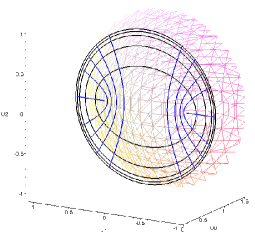
Figure 9: Projective plane for elliptic system is formed by ellipses and convex hyperbolas

and it coincides with the known from literature definition of elliptic system of coordinates on hyperboloid $H_{2}$ [20, 67]. Parameters $a_{i}$ $(i=1,2,3)$ define the positions of two foci for co-focal ellipses and hyperbolas on $H_{2}$ (see Fig. 9). One can obtain its coordinates making $\rho_{1}\to a_{1}$ and $\rho_{2}\to a_{1}$, then $F_{1,2}\left(u_{0},\pm u_{1},u_{2}\right)\equiv F_{1,2}\left(R\frac{1}{k},\pm R\frac{k^{\prime}}{k},0\right)$, where

$${k^{\prime}}^{2}=\frac{a_{1}-a_{2}}{a_{1}-a_{3}},\qquad{k}^{2}=\frac{a_{2}-a_{3}}{a_{1}-a_{3}},$$ (150)

where $\sinh^{2}\beta=\frac{{k^{\prime}}^{2}}{{k}^{2}}$ and $2\beta R$ is the distance between the foci. Elliptic coordinates (149) are given in algebraic form and they actually depend on the three parameters $a_{i}$. Equivalently to this form we can define the elliptic system in terms of Jacobi elliptic functions which depend on just one parameter. It frees us from ambiguity in determining the position of a point on hyperboloid $H_{2}$ in terms of elliptic coordinates.

If we put [20, 67]:

$$\rho_{1}=a_{1}-(a_{1}-a_{3})\mbox{dn}^{2}(a,k),\qquad\rho_{2}=a_{1}-(a_{1}-a_{2})\mbox{sn}^{2}(b,k^{\prime}),$$ (151)

into expression (149), where functions $\mbox{sn}(a,k)$, $\mbox{cn}(a,k)$ and $\mbox{dn}(a,k)$ are Jacobi elliptic functions with modulus $k$ and $k^{\prime}$ [6] related by well known identities $\mbox{sn}^{2}(a,k)+\mbox{cn}^{2}(a,k)=1$ and $k^{2}\mbox{sn}^{2}(a,k)+\mbox{dn}^{2}(a,k)=1$, we obtain Jacobi form of the elliptic coordinates

$$u_{0}=R\mbox{sn}(a,k)\mbox{dn}(b,k^{\prime}),\ u_{1}=iR\mbox{cn}(a,k)\mbox{cn}(b,k^{\prime}),\ u_{2}=iR\mbox{dn}(a,k)\mbox{sn}(b,k^{\prime}),$$ (152)

where $a\in\left(iK^{\prime},iK^{\prime}+2K\right)$, $b\in\left[0,4K^{\prime}\right)$, $k^{2}+{k^{\prime}}^{2}=1$, $K=K(k)$, $K^{\prime}=K(k^{\prime})$ are complete elliptic integrals with $k$ and ${k^{\prime}}$, respectively. Jacobi elliptic functions degenerate into trigonometric or hyperbolic functions if one of the periods is infinite, i.e. modulus $k^{2}$ is zero or one [6]. In the limiting case $k^{2}\to 1$, $k^{\prime 2}\to 0$ we have that $K\sim\infty$, $K^{\prime}\sim\frac{\pi}{2}$ and

$$\mbox{sn}(\mu,k)\to\tanh\mu,\qquad\mbox{dn}(\mu,k)\to\frac{1}{\cosh\mu},$$ (153)

whereas for limit $k^{2}\to 0$, $k^{\prime 2}\to 1$ we have $K\sim\frac{\pi}{2}$, $K^{\prime}\sim\infty$ and

$$\mbox{sn}(\mu,k)\to\sin\mu,\qquad\mbox{dn}(\mu,k)\to 1.$$ (154)

2.   For the one-sheeted hyperboloid inequality (117) holds over the whole space. Thus we can construct in the same way as in (149) the elliptic system of coordinates (Fig. 32)

$$u_{0}^{2}=R^{2}{\frac{\left({\rho_{1}}-{a_{3}}\right)\left({a_{3}}-{\rho_{2}}\right)}{\left({a_{1}}-{a_{3}}\right)\left({a_{2}}-{a_{3}}\right)}},\quad u_{1}^{2}=R^{2}{\frac{\left({\rho_{1}}-{a_{2}}\right)\left({a_{2}}-{\rho_{2}}\right)}{\left({a_{1}}-{a_{2}}\right)\left({a_{2}}-{a_{3}}\right)}},\quad u_{2}^{2}=R^{2}{\frac{\left({a_{1}}-{\rho_{1}}\right)\left(a_{1}-\rho_{2}\right)}{\left({a_{1}}-{a_{2}}\right)\left({a_{1}}-{a_{3}}\right)}},$$ (155)

where now $\rho_{2}<a_{3}<a_{2}<\rho_{1}<a_{1}$. Introducing Jacobi functions as in (151) we can rewrite coordinates (155) in form

$$u_{0}=iR\mbox{sn}(a,k)\mbox{dn}(b,k^{\prime}),\quad u_{1}=-R\mbox{cn}(a,k)\mbox{cn}(b,k^{\prime}),\quad u_{2}=-R\mbox{dn}(a,k)\mbox{sn}(b,k^{\prime}),$$ (156)

where now $a\in[K,K+i4K^{\prime})$ and $b\in(iK,iK+2K^{\prime})$.

Let us finally note that the elliptic systems of coordinates are an one-parametric coordinate systems depending on $k$ and in the limit $k\to 0$ (respectively $k\to 1$) the subgroup coordinate systems arise. Indeed, in the case when $\beta\to 0$ (or $k\to 1$): $S_{E}\sim L^{2}$ and we get that the elliptic coordinates transform into the spherical ones, whereas for the large $\beta\sim\infty$ ($k\to 0$): $S_{E}/\sinh^{2}\beta\sim K^{2}_{2}$ we obtain the equidistant coordinates. To track these limits directly on the level of coordinates, let us use some properties of Jacobi functions and complete elliptic integrals in (153) and (154). Firstly let us consider the two-sheeted hyperboloid. In the limiting case $k\to 1$, i.e., $k^{\prime}\to 0$ we obtain

$$\begin{array}[]{ll}\mbox{sn}(a,k)\to\tanh(i\pi/2+\mu)=\coth\mu\equiv\cosh\tau,&\mbox{dn}(a,k)\to\frac{1}{\cosh(i\pi/2+\mu)}=-\frac{i}{\sinh\mu}\equiv\sinh\tau,\\[8.53581pt] \mbox{sn}(b,k^{\prime})\to\sin b\equiv\sin\varphi,&\mbox{dn}(b,k^{\prime})\to 1,\end{array}$$ (159)

where $\tau\in(0,\infty)$ and $\varphi\in[0,2\pi)$. Therefore the elliptic coordinate system (152) on $H_{2}$ yields spherical coordinates (49).

To determine the second limit $k^{\prime}\to 1$, $k\to 0$, let us introduce new variables $(\nu,\mu)$ through the substitution $a=\nu+iK^{\prime}$ and $b=\mu+K^{\prime}$, where $\nu\in(0,2K)$ and $\mu\in\left[-K^{\prime},3K^{\prime}\right)$. Using the following formulas [6]

$$\begin{array}[]{lll}\mbox{sn}(\nu+iK^{\prime},k)=\frac{1}{k\mbox{sn}(\nu,k)},&\mbox{cn}(\nu+iK^{\prime},k)=-\frac{i}{k}\frac{\mbox{dn}(\nu,k)}{\mbox{sn}(\nu,k)},&\mbox{dn}(\nu+iK^{\prime},k)=-i\frac{\mbox{cn}(\nu,k)}{\mbox{sn}(\nu,k)},\\[8.53581pt] \mbox{sn}(\mu+K^{\prime},k^{\prime})=\frac{\mbox{cn}(\mu,k^{\prime})}{\mbox{dn}(\mu,k^{\prime})},&\mbox{cn}(\mu+K^{\prime},k^{\prime})=-k\frac{\mbox{sn}(\mu,k^{\prime})}{\mbox{dn}(\mu,k^{\prime})},&\mbox{dn}(\mu+K^{\prime},k^{\prime})=\frac{k}{\mbox{dn}(\mu,k)},\end{array}$$ (162)

taking into account equations (153) and (154), and denoting $\tau_{2}=\mu$ and $\cosh\tau_{1}=1/\sin\nu$ it is easy to reproduce from the elliptic coordinates (152) the equidistant system of coordinates (57).

There is also an alternative way to find the same results. Let us consider equivalent intervals for $a\in\left[K-2iK^{\prime},K+2iK^{\prime}\right)$, $b\in\left(-iK,iK\right)$ (corresponding to order $a_{3}<a_{2}\leq\rho_{1}<a_{1}\leq\rho_{2}$) and making the change of variables $a=\pi/2+i\tau_{2}$, $b=-i\arctan(\sinh\tau_{1})$, from (152) , then for $k^{\prime}\to 1$, $k\to 0$ we obtain equidistant system (57).

For one-sheeted hyperboloid, taking intervals $a\in\left(-iK^{\prime},iK^{\prime}\right)$, $b\in\left[0,4K^{\prime}\right)$ (corresponding to $\rho_{1}<a_{3}<a_{2}<\rho_{2}<a_{1}$) and introducing new variables $a=\tanh^{-1}(-i\sinh\tau)$, $b=\varphi$ one can see that system (156) goes to pseudo spherical one (51), when $k\to 1$, $k^{\prime}\to 0$.

In the case when $k\to 0$, $k^{\prime}\to 1$, introducing $a=\pi/2+i\tau_{2}$, $b=\coth^{-1}(\cosh\tau_{1})+i\pi/2$ and considering intervals $a\in[K,K+i4K^{\prime})$ and $b\in(iK,iK+2K^{\prime})$ from (156) one can obtain equidistant system of Type I (59), with $u_{2}\leqslant-R$, $\tau_{1}\in\mathbb{R}$, $\tau_{2}\in\mathbb{R}^{+}$. To obtain the second part of equidistant system, when $u_{2}\geqslant R$ one can consider the alternative interval $b\in(iK-2K^{\prime},iK)$ taking $b=\coth^{-1}(-\cosh\tau_{1})+i\pi/2$.

Finally, taking $a\in\left(-iK^{\prime},iK^{\prime}\right)$, $b\in\left[0,4K^{\prime}\right)$ and $a=i\tau$, $b=\mbox{arccosh}(-1/\sin\varphi)$ we obtain from (156) the equidistant coordinates of Type Ib (62) with $\varphi\in[\pi,2\pi)$ that corresponds to $u_{1}\leqslant 0$.

2.9 Rotated elliptic system of coordinates

The rotated elliptic system of coordinates corresponding to operator $S_{\tilde{E}}=\cosh 2\beta L^{2}+1/2\sinh 2\beta\{K_{1},L\}$ (see (97) and (28)) can be obtained from the elliptic system (152) through hyperbolic rotation with angle $\beta$ about axis $u_{2}$:

$$\left({{\begin{array}[]{*{20}c}u^{\prime}_{0}\\ u^{\prime}_{1}\\ u^{\prime}_{2}\end{array}}}\right)=\left({{\begin{array}[]{*{20}c}\cosh\beta&\sinh\beta&0\\ \sinh\beta&\cosh\beta&0\\ 0&0&1\end{array}}}\right)\left({{\begin{array}[]{*{20}c}u_{0}\\ u_{1}\\ u_{2}\end{array}}}\right)=\left({{\begin{array}[]{*{20}c}u_{0}\cosh\beta+u_{1}\sinh\beta\\ u_{0}\sinh\beta+u_{1}\cosh\beta\\ u_{2}\end{array}}}\right)$$ (163)

Substituting now equation (152) in (163) we obtain

$$u^{\prime}_{0} = \frac{R}{k}\left\{\mbox{sn}(a,k)\mbox{dn}(b,k^{\prime})+ik^{\prime}\mbox{cn}(a,k)\mbox{cn}(b,k^{\prime})\right\},$$

$$u^{\prime}_{1} = \frac{R}{k}\left\{k^{\prime}\mbox{sn}(a,k)\mbox{dn}(b,k^{\prime})+i\mbox{cn}(a,k)\mbox{cn}(b,k^{\prime})\right\},$$ (164)

$$u^{\prime}_{2} = iR\mbox{dn}(a,k)\mbox{sn}(b,k^{\prime}),$$

where intervals for $a$, $b$ are the same as in (152). This system of coordinates was introduced for the first time in article [20] to provide the separation of variables in Schrodinger equation with Coulomb potential on two-dimensional two-sheeted hyperboloid.

We do not introduce here the analog of rotated elliptic system of coordinates on the one-sheeted hyperboloid because this system does not lead to the new contraction on the pseudo-euclidean space $E_{1,1}$.

2.10 Hyperbolic system of coordinates

1. For operator $S_{H}=K_{2}^{2}-\sin^{2}\alpha L^{2}$, $\sin^{2}\alpha\neq 0,\neq 1$ system (116) looks as follows

$$\lambda_{1}+\lambda_{2}=u_{1}^{2}\sin^{2}\alpha-u_{2}^{2}\cos^{2}\alpha-R^{2},\quad\lambda_{1}\lambda_{2}=-R^{2}u_{1}^{2}\sin^{2}\alpha,$$ (165)

and it has the solution

$$u_{0}^{2}=-\frac{\left({\lambda_{1}}+{R^{2}}\sin^{2}\alpha\right)\left({\lambda_{2}}+{R^{2}}\sin^{2}\alpha\right)}{R^{2}\sin^{2}\alpha\cos^{2}\alpha},\quad u_{1}^{2}=-\frac{\lambda_{1}\lambda_{2}}{R^{2}\sin^{2}\alpha},\quad u_{2}^{2}=-\frac{\left({\lambda_{1}}+{R^{2}}\right)\left({\lambda_{2}}+{R^{2}}\right)}{R^{2}\cos^{2}\alpha},$$ (166)

where $\lambda_{1}\leq-R^{2}<0\leq\lambda_{2}$. Introducing now new constants $a_{3}<a_{2}<a_{1}$ such that $\sin^{2}\alpha=(a_{2}-a_{3})/(a_{1}-a_{3})$ and making the change of variables: $\lambda_{2}/R^{2}=\frac{a_{3}-\rho_{2}}{a_{1}-a_{3}}$, $\lambda_{1}/R^{2}=\frac{a_{3}-\rho_{1}}{a_{1}-a_{3}}$, we obtain the algebraic form of hyperbolic system of coordinates (Fig. 13)

$$u_{0}^{2}=R^{2}{\frac{\left({\rho_{1}}-{a_{2}}\right)\left({a_{2}-\rho_{2}}\right)}{\left({a_{1}}-{a_{2}}\right)\left({a_{2}}-{a_{3}}\right)}},\quad u_{1}^{2}=R^{2}{\frac{\left({\rho_{1}}-{a_{3}}\right)\left({a_{3}-\rho_{2}}\right)}{\left({a_{1}}-{a_{3}}\right)\left({a_{2}}-{a_{3}}\right)}},\quad u_{2}^{2}=R^{2}{\frac{\left({\rho_{1}}-{a_{1}}\right)\left({a_{1}-\rho_{2}}\right)}{\left({a_{1}}-{a_{2}}\right)\left({a_{1}}-{a_{3}}\right)}},$$ (167)

with $\rho_{2}<a_{3}<a_{2}<a_{1}<\rho_{1}$.

After putting formula (151) in (167), where moduli $k$ and $k^{\prime}$ are the same as in formula (150), we obtain

$$u_{0}=-R\mbox{cn}(a,k)\mbox{cn}(b,k^{\prime}),\qquad u_{1}=iR\mbox{sn}(a,k)\mbox{dn}(b,k^{\prime}),\qquad u_{2}=iR\mbox{dn}(a,k)\mbox{sn}(b,k^{\prime}).$$ (168)

where $a\in\left(iK,iK+2K\right)$, $b\in\left(iK,iK+2K^{\prime}\right)$.

2. The case of one-sheeted hyperboloid is more complicated. From relation (117) we obtain that the covered parts of hyperboloid are defined by the following inequality

$$|u_{1}^{2}\sin^{2}\alpha-u_{2}^{2}\cos^{2}\alpha+R^{2}|>2R|u_{1}\sin\alpha|.$$ (169)

The same procedure as in the previous case gives us the hyperbolic system of coordinates on one-sheeted hyperboloid in form (Fig. 34)

$$u_{0}^{2}=R^{2}{\frac{\left({\rho_{1}}-{a_{2}}\right)\left({\rho_{2}-a_{2}}\right)}{\left({a_{1}}-{a_{2}}\right)\left({a_{2}}-{a_{3}}\right)}},\quad u_{1}^{2}=R^{2}{\frac{\left({\rho_{1}}-{a_{3}}\right)\left({\rho_{2}-a_{3}}\right)}{\left({a_{1}}-{a_{3}}\right)\left({a_{2}}-{a_{3}}\right)}},\quad u_{2}^{2}=R^{2}{\frac{\left({\rho_{1}}-{a_{1}}\right)\left({\rho_{2}-a_{1}}\right)}{\left({a_{1}}-{a_{2}}\right)\left({a_{1}}-{a_{3}}\right)}},$$ (170)

where it is necessary to select two cases:

• Hyperbolic Type I $H_{I}^{A}:$ $\rho_{1}$, $\rho_{2}<a_{3}<a_{2}<a_{1}$ ($H_{I}^{B}:$ $a_{3}<a_{2}<a_{1}<\rho_{1}$, $\rho_{2}$),

• Hyperbolic Type II $H_{II}^{A}:$ $a_{3}<\rho_{1},\rho_{2}<a_{2}<a_{1}$ ($H_{II}^{B}:$ $a_{3}<a_{2}<\rho_{1},\rho_{2}<a_{1}$).

It means that the covered part of one-sheeted hyperboloid (169) is splitting into several sub-parts corresponding to each type of the system as presented in Fig. 34.

It is more convenient for us to rewrite coordinates (170) in the form of Jacobi elliptic functions. Introducing Jacobi functions as in (151) with the same moduli $k$ and $k^{\prime}$, given by formula (150), we come to

$$u_{0}=-iR\mbox{cn}(a,k)\mbox{cn}(b,k^{\prime}),\qquad u_{1}=-R\mbox{sn}(a,k)\mbox{dn}(b,k^{\prime}),\qquad u_{2}=-R\mbox{dn}(a,k)\mbox{sn}(b,k^{\prime}).$$ (171)

It is easy to verify that angles $a$, $b$ run the intervals

$$\text{for }H_{I}^{A}:\ a\in(-iK^{\prime},iK^{\prime}),\quad b\in\left(iK,iK+2K^{\prime}\right);$$

$$\text{for }H_{I}^{B}:\ a\in(iK^{\prime},iK^{\prime}+2K),\quad b\in\left(-iK,iK\right);$$

$$\text{for }H_{II}^{A}:\ a\in\left[0,4K\right),\quad b\in\left[K^{\prime},K^{\prime}+i4K\right);$$

$$\text{for }H_{II}^{B}:\ a\in[K,K+i4K^{\prime}),\quad b\in\left[0,4K^{\prime}\right).$$

Let us note that in general (except the particular case $k=k^{\prime}$) systems $H^{B}$ could not be obtained from $H^{A}$ through trigonometric rotation on $\pi/2$ over $u_{0}$. One can observe that system $H_{I}^{A}$ is divided geometrically into four parts depending on the sign of $u_{0}$ and $u_{2}$, so it is necessary to choose the appropriate sign for these coordinates. The same is true for $H_{I}^{B}$. As for $H_{II}^{A}$ here we have two parts depending on the sign of $u_{2}$ and for $H_{II}^{B}$ one should select the sign of $u_{1}$.

Let us note, that families of coordinate curves $\rho_{i}=\text{const.}$ have straight lines as envelopes defined by the equalities

$$|ku_{1}\pm R|=k^{\prime}|u_{2}|$$ (173)

with intersections in the limit points $(0,\pm kR,\pm k^{\prime}R)$, $(\pm Rk/k^{\prime},0,\pm R/k^{\prime})$, $(\pm Rk^{\prime}/k\pm R/k,0)$. To avoid the intersection of coordinate curves on one family, it is necessary to take the points of envelops as initial ones for one family and as endpoints for the other family. For example, for system $H_{I}^{A}$ if we consider fixed $\rho_{1}=\rho_{10}=\text{const.}$, then $\rho_{2}$ should be in the interval $\rho_{2}\in(-\infty,\rho_{10})$ and for fixed $\rho_{2}=\rho_{20}=\text{const.}$ the corresponding interval is $\rho_{1}\in(\rho_{20},a_{3})$.

In the limit case, when $k=\sin\alpha\to 0$ ($k^{\prime}\to 1$) operator $S_{H}=K_{2}^{2}-\sin^{2}\alpha L^{2}$ goes to equidistant one $K_{2}^{2}$. When $k^{\prime}\to 0$, considering $S_{SH}-{\cal C}=-K_{1}^{2}+L^{2}{k^{\prime}}^{2}$ we obtain the rotated equidistant operator $-K_{1}^{2}$.

For system (168) on two-sheeted hyperboloid, taking $a\in\left(2K-iK^{\prime},2K+iK^{\prime}\right)$, $b\in(-iK,iK)$ and introducing variables $\alpha=\pi+i\tau_{2}$, $\beta=-i\arctan(\sinh\tau_{1})$ in limit $k\to 0$ one can obtain equidistant system (57).

Let us consider system $H_{I}^{A}$ (171) with $a\in\left(2K-iK^{\prime},2K+iK^{\prime}\right)$, $b\in\left(iK,iK+2K^{\prime}\right)$. Introducing $\alpha=\pi+i\tau_{2}$, $\beta=\tanh^{-1}(\cosh\tau_{1})+i\pi/2$ we obtain equidistant system of Type Ia (59) when $k\to 0$. From $H_{II}^{B}$ with $\alpha=\pi/2-i\tau$, $\beta=\tanh^{-1}(\cos\varphi)$ we come to equidistant system (62) for $a\in\left[K-2iK^{\prime},K+2iK^{\prime}\right)$, $b\in\left[-2K^{\prime},2K^{\prime}\right)$ with the same limit $k\to 0$. By analogy one can consider the contractions of the rest of the systems from (2.10) to corresponding equidistant systems on one-sheeted hyperboloid.

As in the case of rotated elliptic system on the two-sheeted hyperboloid, here we introduce the rotated hyperbolic system. Let us consider hyperbolic rotation (74) through angle $a_{1}=\mbox{arccosh}\left(1/\cos\alpha\right)$ about axis $u_{1}$ (see (28)):

$$\left({{\begin{array}[]{*{20}c}u^{\prime}_{0}\\ u^{\prime}_{1}\\ u^{\prime}_{2}\end{array}}}\right)=\left({{\begin{array}[]{*{20}c}\frac{1}{\cos\alpha}&0&-\frac{\sin\alpha}{\cos\alpha}\\ 0&1&0\\ -\frac{\sin\alpha}{\cos\alpha}&0&\frac{1}{\cos\alpha}\end{array}}}\right)\left({{\begin{array}[]{*{20}c}u_{0}\\ u_{1}\\ u_{2}\end{array}}}\right)=\left({{\begin{array}[]{*{20}c}\frac{u_{0}-u_{2}\sin\alpha}{\cos\alpha}\\ u_{1}\\ \frac{-u_{0}\sin\alpha+u_{2}}{\cos\alpha}\end{array}}}\right),$$ (174)

then

$$K_{2}=\left(K_{2}^{\prime}+\sin\alpha L^{\prime}\right)/\cos\alpha,\quad L=\left(\sin\alpha K_{2}^{\prime}+L^{\prime}\right)/\cos\alpha$$ (175)

and correspondingly operator $S_{H}$ transforms into rotated hyperbolic operator

$$S_{\tilde{H}}=cK_{2}^{2}+\{K_{2},L\},\ c=\sin\alpha+1/\sin\alpha,\ \sin^{2}\alpha\neq 0,1.$$ (176)

For this system of coordinates we get from (171) and (174) (see Fig. 36):

$$u_{0}^{\prime} = \frac{R}{k^{\prime}}\left[k\mbox{dn}(a,k)\mbox{sn}(b,k^{\prime})-i\mbox{cn}(a,k)\mbox{cn}(b,k^{\prime})\right],$$

$$u_{1}^{\prime} = -R\mbox{sn}(a,k)\mbox{dn}(b,k^{\prime}),$$ (177)

$$u_{2}^{\prime} = \frac{R}{k^{\prime}}\left[ik\mbox{cn}(a,k)\mbox{cn}(b,k^{\prime})-\mbox{dn}(a,k)\mbox{sn}(b,k^{\prime})\right],$$

with intervals for $a$ and $b$ as in (2.10). The reason for introducing rotated hyperbolic system of coordinates is the construction of another contraction limits showed later.

3 Contractions on Two-Sheeted Hyperboloid

3.1 Contraction of Lie algebra $so(2,1)$ to $e(2)$

To realize the contractions of Lie algebra $so(2,1)$ to $e(2)$ let us introduce Beltrami coordinates on the hyperboloid $H_{2}$ in such a way

$$x_{\mu}=R\frac{u_{\mu}}{u_{0}}=R\frac{u_{\mu}}{\sqrt{R^{2}+u_{1}^{2}+u_{2}^{2}}},\qquad\qquad\mu=1,2.$$ (178)

In terms of variables (178) generators (2) look like this

$$-\frac{K_{1}}{R}\equiv\pi_{2} = \partial_{x_{2}}-\frac{x_{2}}{R^{2}}(x_{1}\partial_{x_{1}}+x_{2}\partial_{x_{2}}),$$

$$-\frac{K_{2}}{R}\equiv\pi_{1} = \partial_{x_{1}}-\frac{x_{1}}{R^{2}}(x_{1}\partial_{x_{1}}+x_{2}\partial_{x_{2}}),$$ (179)

$$L = x_{1}\partial_{x_{2}}-x_{2}\partial_{x_{1}}=x_{1}\pi_{2}-x_{2}\pi_{1}$$

and commutator relations of $so(2,1)$ take the form

$$[\pi_{1},\pi_{2}]=\frac{L}{R^{2}},\ [\pi_{1},L]=\pi_{2},\ [L,\pi_{2}]=\pi_{1}.$$ (180)

Let us take the basis of $e(2)$ in the form

$$p_{1}=\partial_{x_{1}},\qquad p_{2}=\partial_{x_{2}},\qquad M=x_{2}\partial_{x_{1}}-x_{1}\partial_{x_{2}},$$ (181)

with commutators

$$[p_{1},p_{2}]=0,\qquad[p_{1},M]=-p_{2},\qquad[M,p_{2}]=-p_{1}.$$ (182)

Then in limit $R^{-1}\to 0$ we have

$$\pi_{1}\to p_{1},\qquad\pi_{2}\to p_{2},\qquad L\to-M,$$ (183)

relations (180) contract to (182), so algebra $so(2,1)$ contracts to $e(2)$. Moreover, Laplace-Beltrami operator of $so(2,1)$ contracts to operator of $e(2)$:

$$\Delta_{LB}=\frac{1}{R^{2}}(K_{1}^{2}+K_{2}^{2}-L^{2})=\pi_{1}^{2}+\pi_{2}^{2}-\frac{M^{2}}{R^{2}}\to\Delta=p_{1}^{2}+p_{2}^{2}.$$ (184)

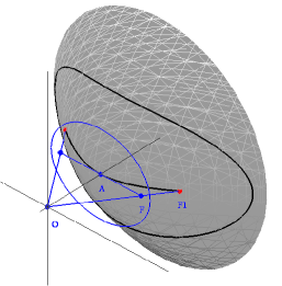
Figure 1: Projective plane for two-sheeted hyperboloid

3.2 Contractions of the systems of coordinates

In the case of hyperboloid $H_{2}$ Beltrami coordinates (178) are coordinates $(x_{1},x_{2})$ on the projective plane $u_{0}=R$ in the interior of circle $x_{1}^{2}+x_{2}^{2}=R^{2}$ (inhomogeneous or projective coordinates, see Fig. 1). In contraction limit $R\to\infty$ this circle is transformed to euclidean plane $E_{2}$. It allows to relate the coordinate systems on $H_{2}$ to the corresponding ones on $E_{2}$.

The metric for projective plane $(x_{1},x_{2})$ induced by the metric on two-sheeted hyperboloid, has the form

$$ds^{2}=\left(1-\frac{x_{1}^{2}+x_{2}^{2}}{R^{2}}\right)^{-2}\left[\left(1-\frac{x_{2}^{2}}{R^{2}}\right)dx_{1}^{2}+2\frac{x_{1}x_{2}}{R^{2}}dx_{1}dx_{2}+\left(1-\frac{x_{1}^{2}}{R^{2}}\right)dx_{2}^{2}\right]$$ (185)

and contracts to the metric on euclidean plane $ds^{2}=dx_{1}^{2}+dx_{2}^{2}\sim dx^{2}+dy^{2}$.

3.3 Contractions of nonorthogonal systems

1. Considering nonorthogonal pseudo-spherical system (50) for the fixed geodesic parameter $r=\tau R$, we obtain that $\tau\sim r/R$ when $R\to\infty$. Beltarmi coordinates contract as follows:

$$x_{1}=R\frac{u_{1}}{u_{0}}=R\tanh\tau\cos\left(\varphi+\frac{R\tau}{\alpha}\right)\rightarrow r\cos\left(\varphi+\frac{r}{\alpha}\right),$$

$$x_{2}=R\frac{u_{2}}{u_{0}}=R\tanh\tau\sin\left(\varphi+\frac{R\tau}{\alpha}\right)\rightarrow r\sin\left(\varphi+\frac{r}{\alpha}\right),$$

so we get nonorthogonal polar coordinates on euclidean plane $E_{2}$ (see Table 4). For corresponding operator we obtain $-S_{SPH}=-L\to M=y\partial_{x}-x\partial_{y}=X_{S}$.

2. For nonorthogonal equidistant system (58), taking $\tau_{1}\sim y^{\prime}/R$, $\tau_{2}\sim x^{\prime}/R$, $\alpha\sim R$ we obtain:

$$x_{1}=R\frac{u_{1}}{u_{0}}=R\tanh(R\tau_{1}/\alpha+\tau_{2})\rightarrow x^{\prime}+y^{\prime},\qquad x_{2}=R\frac{u_{2}}{u_{0}}=R\frac{\tanh(R\tau_{1}/\alpha)}{\cosh\tau_{2}}\rightarrow y^{\prime},$$

where $(x^{\prime},y^{\prime})$ are nonorthogonal Cartesian coordinates on $E_{2}$ (Table 4). For symmetry operator we have $-S_{EQ}/R=-K_{2}/R\to p_{1}=X_{C}$.

3. Let us consider nonorthogonal horicyclic system (69) in permuted form $u_{1}\leftrightarrow u_{2}$. Then in contraction limit one can obtain nonorthogonal Cartesian coordinates $(x^{\prime},y^{\prime})$, if $\tilde{x}\sim y^{\prime}/R$, $\tilde{y}\sim 1+x^{\prime}/R$. For corresponding Beltrami coordinates we have:

$$x_{1}\to x^{\prime}+y^{\prime},\qquad x_{2}\to x^{\prime}$$

and $-S_{\bar{HO}}/R=(-K_{2}+L)/R=\pi_{1}+L/R\to p_{1}=X_{C}$.

3.4 Pseudo-spherical to polar

Figure 2: Spherical system

Figure 3: Projective plane for spherical system is formed by circles and straight lines passing through the center

For pseudo-spherical coordinate system (49) we fix the geodesic parameter $r=\tau R$. Then, if $R^{-1}$ tends to zero, then $\tau\to 0$ $\tanh\tau\simeq\tau\simeq\frac{r}{R}$. In the limit for Beltrami coordinates we have

$$x_{1}=R\frac{u_{1}}{u_{0}}=R\tanh\tau\cos\varphi\rightarrow r\cos\varphi,\qquad x_{2}=R\frac{u_{2}}{u_{0}}R\tanh\tau\sin\varphi\rightarrow r\sin\varphi.$$

Thus the pseudo-spherical coordinates on $H_{2}$ contract into polar coordinates $(r,\varphi)$ on the euclidean plane $E_{2}$ (see Table 4). For the corresponding pseudo-spherical operator we obtain $S_{SPH}^{(2)}=L^{2}\to M^{2}=X^{2}_{S}$.

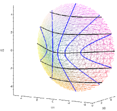
Figure 4: Equidistant system

3.5 Equidistant to Cartesian

For equidistant system of coordinates (57) Beltrami coordinates (178) look like

$$x_{1}=R\tanh\tau_{2},\qquad x_{2}=R\tanh\tau_{1}/\cosh\tau_{2}.$$

Taking limit $R^{-1}\to 0$, $\tau_{1}\to 0$, $\tau_{2}\to 0$ and putting $\sinh\tau_{1}\simeq y/R$, $\sinh\tau_{2}\simeq x/R$ we get

$$x_{1}\rightarrow x,\qquad x_{2}\rightarrow y$$

and

$$\frac{S_{EQ}^{(2)}}{R^{2}}=\frac{K_{2}^{2}}{R^{2}}\to p_{1}^{2}=X_{C}^{2},$$

where $(x,y)$ are the orthogonal Cartesian coordinates on euclidean plane $E_{2}$ (see Table 4).

3.6 Horicyclic to Cartesian

For horicyclic variables $\tilde{x}$, $\tilde{y}$ (68) we have

$$\tilde{x}=\frac{u_{2}}{u_{0}-u_{1}},\qquad\qquad\tilde{y}=\frac{R}{u_{0}-u_{1}}.$$

In contraction limit $R\to\infty$ we obtain

$$\tilde{x}\to\frac{y}{R},\qquad\qquad\tilde{y}\to 1+\frac{x}{R},$$

and Beltrami coordinates are transforming to Cartesian ones:

$$x_{1}=R\frac{\tilde{x}^{2}+\tilde{y}^{2}-1}{\tilde{x}^{2}+\tilde{y}^{2}+1}\to x,\qquad x_{2}=R\frac{2\tilde{x}}{\tilde{x}^{2}+\tilde{y}^{2}+1}\to y.$$

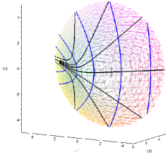
Figure 6: Horicyclic system

Figure 7: Projective plane for horicyclic system is formed by straight lines passing through the boundary point and horicycles

For the corresponding operator $S_{HO}^{(2)}$ we get

$$\frac{S_{HO}^{(2)}}{R^{2}}=\frac{(K_{1}+L)^{2}}{R^{2}}=\pi_{2}^{2}+\frac{L^{2}}{R^{2}}-\frac{1}{R}\{\pi_{2},L\}\to p_{2}^{2}\simeq X_{C}^{2}.$$

3.7 Elliptic coordinates to elliptic, Cartesian, polar and parabolic ones

On the projective plane the ellipse foci of (149) have coordinates $F\left(\pm R\tan\alpha,0\right)$ where $\tan^{2}\alpha=(a_{1}-a_{2})/(a_{1}-a_{3})$ and $\alpha$ is angle $AOF$ (see Fig. 1). The same points are the foci for hyperbolas. We must distinguish three cases for limit $R\to\infty$, namely: when the length of $AF$ is fixed and $\alpha\to 0$, when $AF$ and $\alpha$ go to zero, and when $\alpha$ is fixed and $AF\to\infty$. The latter limiting procedure involves two additional cases when one or two foci go to infinity with pseudo-radius $R$.

3.7.1 Elliptic to elliptic

Let us introduce parameter $D=\sqrt{a_{1}-a_{2}}$ that defines the focal distance for elliptic coordinate system on $E_{2}$ plane. The value of $D$ is the limit one for the length of arc $AF_{1}$, as well for the length of $AF$, when $R\to\infty$ (see Fig. 1). Therefore, for the fixed values of $D$ in contraction limit $-a_{3}\simeq R^{2}\to\infty$ we get

$$\sinh^{2}\beta=\frac{a_{1}-a_{2}}{a_{2}-a_{3}}\simeq\frac{D^{2}}{R^{2}}\to 0,$$ (186)

and

$$S_{E}=L^{2}+\sinh^{2}\beta K_{2}^{2}=L^{2}+R^{2}\sinh^{2}\beta\pi_{1}^{2}\to M^{2}+D^{2}p_{1}^{2}=X_{E}.$$

Introducing new variables $\xi$ and $\eta$ as

$$\sinh^{2}\xi=\frac{\rho_{1}-a_{1}}{a_{1}-a_{2}},\qquad\cos^{2}\eta=\frac{\rho_{2}-a_{2}}{a_{1}-a_{2}},\qquad\xi\in[0,\infty),\quad\eta\in[0,2\pi),$$

we can rewrite the elliptic system of coordinates (149) in the form

$$u_{0}^{2} = R^{2}\left[1+\frac{a_{1}-a_{2}}{a_{1}-a_{3}}\sinh^{2}\xi\right]\left[1+\frac{a_{1}-a_{2}}{a_{2}-a_{3}}\cos^{2}\eta\right],$$

$$u_{1}^{2} = \frac{R^{2}D^{2}}{a_{2}-a_{3}}\cos^{2}\eta\cosh^{2}\xi,$$

$$u_{2}^{2} = \frac{R^{2}D^{2}}{a_{1}-a_{3}}\sin^{2}\eta\sinh^{2}\xi.$$

Taking now limit $-a_{3}\simeq R^{2}\to\infty$ and using relation (186) it is easy to see that Beltrami coordinates

$$x_{1}=R\frac{u_{1}}{u_{0}}\to D\cos\eta\cosh\xi,\quad x_{2}=R\frac{u_{2}}{u_{0}}\to D\sin\eta\sinh\xi$$

contract to the ordinary elliptic coordinates on euclidean plane $E_{2}$ (see Table 4).

Figure 8: Elliptic system

3.7.2 Elliptic to polar

Let us consider the case when $a_{1}-a_{2}\simeq 1/R^{2}$, $a_{2}-a_{3}\simeq R^{2}$, then

$$\sinh^{2}\beta=\frac{a_{1}-a_{2}}{a_{2}-a_{3}}\simeq\frac{1}{R^{4}}.$$

Geometrically it means that foci coincide as $R\to\infty$. Thus for operator $S_{E}$ we have

$$S_{E}\simeq L^{2}+\frac{1}{R^{2}}\pi_{1}^{2}\to M^{2}=X_{S}^{2}.$$

Let us introduce new variables

$$r^{2}=\rho_{1}-a_{2},\qquad\cos^{2}\varphi=\frac{\rho_{2}-a_{2}}{a_{1}-a_{2}}.$$

Then Beltrami coordinates take the form

$$x_{1}^{2}=\frac{(a_{1}-a_{3})}{R^{2}}\frac{r^{2}\cos^{2}\varphi}{(1+r^{2}/R^{2})(1+\cos^{2}\varphi/R^{4})},\qquad x_{2}^{2}=\frac{(a_{2}-a_{3})}{R^{2}}\frac{\sin^{2}\varphi(r^{2}-1/R^{2})}{(1+r^{2}/R^{2})(1+\cos^{2}\varphi/R^{4})}$$

and in limit $(a_{2}-a_{3})\simeq(a_{1}-a_{3})\simeq R^{2}\to\infty$ we obtain

$$x_{1}^{2}\to r^{2}\cos^{2}\varphi,\qquad x_{2}^{2}\to r^{2}\sin^{2}\varphi$$

that coincide with the orthogonal polar coordinates on euclidean plane $E_{2}$ (Table 4).

3.7.3 Elliptic to Cartesian

Let us fix angle $\alpha$ (i.e. the length of $AF$ tends to infinity when $R\to\infty$) and $a_{1}-a_{2}=a_{2}-a_{3}$ (or $k^{2}=k^{{\prime}2}=1/2$). Then we get

$$\frac{S_{E}}{R^{2}}=\frac{1}{R^{2}}(L^{2}+K_{2}^{2})=\frac{L^{2}}{R^{2}}+\pi_{1}^{2}\to p_{1}^{2}=X_{C}^{2}.$$

Taking into account that from (152)

$$-\mbox{cn}^{2}a=\frac{1}{2}\left\{\frac{u_{0}^{2}+u_{2}^{2}}{R^{2}}+\sqrt{\left(\frac{u_{0}^{2}+u_{2}^{2}}{R^{2}}\right)^{2}-\frac{4u_{1}^{2}}{R^{2}}}\right\},\qquad\mbox{cn}^{2}b=\frac{1}{2}\left\{\frac{u_{0}^{2}+u_{2}^{2}}{R^{2}}-\sqrt{\left(\frac{u_{0}^{2}+u_{2}^{2}}{R^{2}}\right)^{2}-\frac{4u_{1}^{2}}{R^{2}}}\right\},$$

we obtain for the large $R$:

$$\mbox{dn}\,a\to-i\frac{y}{R},\ \mbox{cn}\,a\to-i\left(1+\frac{y^{2}}{R^{2}}\right),\ \mbox{sn}\,a\to\sqrt{2}\left(1+\frac{y^{2}}{4R^{2}}\right);$$

$$\mbox{dn}\,b\to\frac{1}{\sqrt{2}}\left(1+\frac{x^{2}}{2R^{2}}\right),\ \mbox{cn}\,b\to\frac{x}{R},\ \mbox{sn}\,b\to 1-\frac{x^{2}}{2R^{2}}.$$

Thus, in contraction limit $R\to\infty$ we get that Beltrami coordinates (178) take Cartesian form:

$$x_{1}=R\frac{i\mbox{cn}\,a\,\mbox{cn}\,b}{\mbox{sn}\,a\,\mbox{dn}\,b}\to x,\qquad x_{2}=R\frac{i\mbox{dn}\,a\,\mbox{sn}\,b}{\mbox{sn}\,a\,\mbox{dn}\,b}\to y.$$

3.7.4 Rotated elliptic to parabolic

The geometrical difference between elliptic system and the rotated elliptic one is the positions of the foci of ellipses. For the rotated elliptic system (see Fig. 11) one of the foci is in $(R^{2},0,0)$. Let us fix constants $a_{i}$ in such a way: $a_{1}-a_{2}=a_{2}-a_{3}$. Then rotating elliptic coordinates (2.9) take the form

$$u^{\prime}_{0}=R\left\{\sqrt{2}\,\mbox{sn}\,a\,\mbox{dn}\,b+i\,\mbox{cn}\,a\,\mbox{cn}\,b\right\},\quad u^{\prime}_{1}=R\left\{\mbox{sn}\,a\,\mbox{dn}\,b+i\sqrt{2}\,\mbox{cn}\,a\,\mbox{cn}\,b\right\},\quad u^{\prime}_{2}=iR\,\mbox{dn}\,a\,\mbox{sn}\,b,$$

with moduli $k=k^{\prime}=1/\sqrt{2}$ for all Jacobi functions. For the large $R$ we obtain

$$\begin{array}[]{ll}\i\mbox{cn}a=\frac{1}{2}\sqrt{\left(1+\sqrt{2}\frac{u^{\prime}_{1}}{R}-\frac{u^{\prime}_{0}}{R}\right)^{2}+2\frac{{u^{\prime}_{2}}^{2}}{R^{2}}}-\frac{1}{2}\sqrt{\left(1-\sqrt{2}\frac{u^{\prime}_{1}}{R}+\frac{u^{\prime}_{0}}{R}\right)^{2}+2\frac{{u^{\prime}_{2}}^{2}}{R^{2}}}\simeq-1+\frac{\sqrt{2}}{2}\frac{u^{2}}{R},\\[8.53581pt] \mbox{cn}b=\frac{1}{2}\sqrt{\left(1+\sqrt{2}\frac{u^{\prime}_{1}}{R}-\frac{u^{\prime}_{0}}{R}\right)^{2}+2\frac{{u^{\prime}_{2}}^{2}}{R^{2}}}+\frac{1}{2}\sqrt{\left(1-\sqrt{2}\frac{u^{\prime}_{1}}{R}+\frac{u^{\prime}_{0}}{R}\right)^{2}+2\frac{{u^{\prime}_{2}}^{2}}{R^{2}}}\simeq 1+\frac{\sqrt{2}}{2}\frac{v^{2}}{R}.\end{array}$$ (187)

For limit $R\to\infty$ we have that Beltrami coordinates go into the parabolic ones:

$$x_{1}\to\frac{u^{2}-v^{2}}{2},\qquad x_{2}\to uv.$$

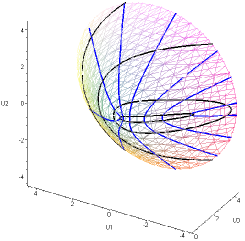
Figure 10: Rotated elliptic system

Figure 11: Projective plane for rotated elliptic system

For the symmetry operator we find

$$\frac{S_{\tilde{E}}}{\sqrt{2}R}=\frac{1}{\sqrt{2}R}\left[\cosh 2\beta L^{2}+1/2\sinh 2\beta\{K_{1},L\}\right]=\frac{3}{\sqrt{2}R}L^{2}-\{\pi_{2},L\}\to\{p_{2},M\}=X_{P}$$

which corresponds to the parabolic coordinates on $E_{2}$ plane (see Table 4).

3.8 Hyperbolic to Cartesian

The hyperbolic system of coordinates (167) is defined by three parameters $a_{1}$, $a_{2}$, $a_{3}$, which fixe the position of the hyperbola foci on hyperboloid. Considering orthogonal projections of coordinates to plane $u_{0}=R$, we obtain the families of hyperbolas. Fixing $\rho_{2}$ for the first family of hyperbolas its minimal focal distance is equal to $2d_{1}$, where $d_{1}=R\sqrt{\frac{a_{1}-a_{3}}{a_{2}-a_{3}}}=\frac{R}{k}$. The minimal focal distance for the second family of hyperbolas (when $\rho_{1}$ is a constant) is equal to $2d_{2}$, where $d_{2}=R\sqrt{\frac{a_{1}-a_{3}}{a_{1}-a_{2}}}=\frac{R}{k^{\prime}}$.

Figure 12: Hyperbolic system

Figure 13: Projective plane for hyperbolic system is formed by concave hyperbolas

If we denote $F_{1}(R,d_{1},0)$, $F_{21}(R,0,d_{2})$ and $F_{22}(R,0,-d_{2})$ then parameter $\sin^{2}\alpha=\frac{a_{2}-a_{3}}{a_{1}-a_{3}}=k^{2}$ where $2\alpha$ is angle $F_{21}F_{1}F_{22}$. Note, that $\sin^{2}\alpha\neq 0,\neq 1$ and one can say that this parameter plays the role of a scale factor for the projective coordinates.

For simplicity let us take $a_{1}-a_{2}=a_{2}-a_{3}$. Then $k^{2}=k^{{\prime}2}=\sin^{2}\alpha=1/2$ and

$$\frac{S_{H}}{R^{2}}=\frac{1}{R^{2}}\left(K_{2}^{2}-\frac{1}{2}L^{2}\right)=\pi_{1}^{2}-\frac{L^{2}}{2R^{2}}\to p_{1}^{2}=X_{C}^{2}.$$

From equation (168) we have

$$\mbox{cn}^{2}a=\frac{1}{2}\left\{\frac{u_{1}^{2}-u_{2}^{2}}{R^{2}}-\sqrt{\left(\frac{u_{1}^{2}-u_{2}^{2}}{R^{2}}\right)^{2}+\frac{4u_{0}^{2}}{R^{2}}}\right\},\qquad-\mbox{cn}^{2}b=\frac{1}{2}\left\{\frac{u_{1}^{2}-u_{2}^{2}}{R^{2}}+\sqrt{\left(\frac{u_{1}^{2}-u_{2}^{2}}{R^{2}}\right)^{2}+\frac{4u_{0}^{2}}{R^{2}}}\right\}.$$

For the large $R$ we get that

$$\mbox{dn}\,a\to-\frac{iy}{R\sqrt{2}},\ \mbox{cn}\,a\to-i\left(1+\frac{y^{2}}{2R^{2}}\right),\ \mbox{sn}\,a\to\sqrt{2}\left(1+\frac{y^{2}}{4R^{2}}\right);$$

$$\mbox{dn}\,b\to-\frac{ix}{R\sqrt{2}},\ \mbox{cn}\,b\to-i\left(1+\frac{x^{2}}{2R^{2}}\right),\ \mbox{sn}\,b\to\sqrt{2}\left(1+\frac{x^{2}}{4R^{2}}\right),$$

and Beltrami coordinates in contraction limit $R\to\infty$ go into Cartesian ones:

$$x_{1}=-iR\frac{\mbox{sn}\,a\ \mbox{dn}\,b}{\mbox{cn}\,a\ \mbox{cn}\,b}\to x,\qquad x_{2}=-iR\frac{\mbox{dn}\,a\ \mbox{sn}\,b}{\mbox{cn}\,a\ \mbox{cn}\,b}\to y.$$ (188)

3.9 Semi-hyperbolic coordinates to Cartesian and parabolic ones

3.9.1 Semi-hyperbolic to Cartesian

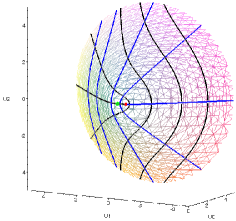
Figure 14: Semi-hyperbolic system

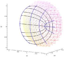
Figure 15: Projective plane for semi-hyperbolic system is formed by semihyperbolas where the focus has coordinates $\left(-R\sqrt{\frac{\sqrt{c^{2}+1}-1}{\sqrt{c^{2}+1}+1}},\,0\right)$.

Let us fix parameter $c=1$ in the semi-hyperbolic system of coordinates (2.4). Then, the coordinates of the focus (see Fig.15) are moved to infinity as $R\to\infty$ and the semi-hyperbolic system of coordinates contracts into Cartesian one. Indeed, if we write out the coordinates $\tau_{1}$, $\tau_{2}$ from (2.4) as

$$\sinh\tau_{1,2}=-\frac{u_{0}u_{1}}{R^{2}}-\frac{1}{2}\left(\frac{u_{2}^{2}}{R^{2}}+1\right)\pm\sqrt{\left(\frac{u_{0}u_{1}}{R^{2}}+\frac{1}{2}\left(\frac{u_{2}^{2}}{R^{2}}+1\right)\right)^{2}+\frac{u_{2}^{2}}{R^{2}}-2\frac{u_{0}u_{1}}{R^{2}}}.$$ (189)

we get for the large $R$

$$\sinh\tau_{1}\to-2\frac{x}{R},\qquad\sinh\tau_{2}\to-1-2\frac{y^{2}}{R^{2}}.$$ (190)

Hence, it is easy to see that at contraction limit $R\to\infty$ Beltrami coordinates go into Cartesian ones: $x_{1}\to x$, $x_{2}\to y$. For the corresponding symmetry operator we obtain

$$\frac{S_{SH}}{R^{2}}=\frac{1}{R^{2}}\left(K_{2}^{2}+\{K_{1},L\}\right)\simeq\pi_{1}^{2}-\frac{1}{R}\{\pi_{2},L\}\to p_{1}^{2}=X_{C}^{2}.$$

3.9.2 Semi-hyperbolic to parabolic

In case of $c=0$, the coordinates of focus $F$ are fixed on the projective plane (see Fig.15) and in the contraction limit $R\to\infty$ the semi-hyperbolic coordinates tend to parabolic ones. Indeed, for variables $\mu_{1,2}$ in (2.4) we have at the large $R$

$$\mu_{1}=\sqrt{\frac{u_{0}^{2}u_{1}^{2}}{R^{4}}+\frac{u_{2}^{2}}{R^{2}}}+\frac{u_{0}u_{1}}{R^{2}}\to\frac{u^{2}}{R},\qquad\mu_{2}=\sqrt{\frac{u_{0}^{2}u_{1}^{2}}{R^{4}}+\frac{u_{2}^{2}}{R^{2}}}-\frac{u_{0}u_{1}}{R^{2}}\to\frac{v^{2}}{R}.$$ (191)

Therefore Beltrami coordinates in limit $R\to\infty$ contract to parabolic ones:

$$x_{1}\to\frac{u^{2}-v^{2}}{2},\qquad x_{2}\to uv.$$ (192)

For symmetry operator $S_{SH}$ we obtain

$$\frac{S_{SH}}{R}=\frac{1}{R}\{K_{1},L\}\to\{p_{2},M\}=X_{P}.$$

3.10 Elliptic-parabolic to Cartesian and parabolic

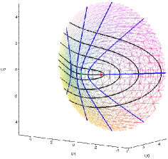
Figure 16: Elliptic-parabolic system

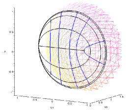
Figure 17: Projective plane for elliptic-parabolic system is formed by elliptic parabolas and convex hyperbolic parabolas. The coordinates of the focus on the projective plane is $\left(R\frac{\gamma-1}{\gamma+1},0\right)$.

3.10.1 Elliptic-parabolic to Cartesian

We start with the case when parameter $\gamma\neq 1$. Then the focus on projective plane (see Fig. 17) moves to infinity as pseudo-radius $R\to\infty$. For variables $\xi_{1}=\cos^{2}\theta$ and $\xi_{2}=\cosh^{2}a$ from (132) we have

$$\xi^{2}_{1,2}=\frac{u_{0}(\gamma+1)+u_{1}(\gamma-1)\mp\sqrt{[u_{0}(\gamma+1)+u_{1}(\gamma-1)]^{2}-4R^{2}\gamma}}{2(u_{0}-u_{1})}.$$ (193)

For the calculation of the behavior of variables $\xi_{1,2}$ at the large $R$, we must distinguish two cases of parameter $\gamma$. For the case of $\gamma\in(0,1)$ we obtain:

$$\cos\theta\to\sqrt{\gamma}\left(1+\frac{x}{R}\right),\qquad\sinh a\to\sqrt{\frac{\gamma}{1-\gamma}}\frac{y}{R},$$ (194)

whereas for $\gamma>1$, we get

$$\sin\theta\to\sqrt{\frac{\gamma}{\gamma-1}}\frac{y}{R},\qquad\cosh a\to\sqrt{\gamma}\left(1+\frac{x}{R}\right).$$ (195)

It is easy to see that in both cases Beltrami coordinates in contraction limit $R\to\infty$ go into Cartesian ones: $x_{1}\to x$, $x_{2}\to y$. For symmetry operator $S_{EP}$ we obtain

$$\frac{1}{(\gamma-1)R^{2}}\left[S_{EP}-R^{2}\Delta_{LB}\right]=\pi_{1}^{2}-\frac{1}{(\gamma-1)R^{2}}\left[R\{\pi_{2},L\}-2L^{2}\right]\to p_{1}^{2}=X_{C}^{2}.$$

3.10.2 Elliptic-parabolic to parabolic

Let us take now $\gamma=1$, then the coordinates of the focus on projective plane are fixed at point $(0,0)$. For the large $R$ we have

$$\sin^{2}\theta=\frac{-u_{1}+\sqrt{u_{0}^{2}-R^{2}}}{u_{0}-u_{1}}\to\frac{v^{2}}{R},\qquad\sinh^{2}a=\frac{u_{1}+\sqrt{u_{0}^{2}-R^{2}}}{u_{0}-u_{1}}\to\frac{u^{2}}{R},$$ (196)

and hence Beltrami coordinates contract into the parabolic ones:

$$x_{1}\to\frac{u^{2}-v^{2}}{2},\qquad x_{2}\to uv.$$ (197)

Symmetry operator $S_{EP}$ transforms as follows

$$\frac{S_{EP}}{R}-R\Delta_{LB}=-\{\pi_{2},L\}+2\frac{L^{2}}{R}\to\{p_{2},M\}=X_{P}.$$

3.11 Hyperbolic-parabolic to Cartesian

Variables $\xi_{1}=\sin\theta$, $\xi_{2}=\sinh b$ from (139) are defined by the following formulas:

$$\xi_{1,2}^{2}=\frac{\pm u_{0}(1-\gamma)\mp u_{1}(\gamma+1)+\sqrt{[u_{0}(\gamma-1)+u_{1}(\gamma+1)]^{2}+4R^{2}\gamma}}{2(u_{0}-u_{1})}.$$ (198)

For the large $R$ we have

$$\cos\theta\to\sqrt{\frac{\gamma}{\gamma+1}}\frac{y}{R},\qquad\sinh b\to\sqrt{\gamma}\left(1+\frac{x}{R}\right).$$ (199)

There is no any special value of $\gamma>0$ (in contrast to the case of elliptic-parabolic system, where contracted variables (194) or (195) have some singularity). Here $\gamma$ is just a scale factor, and Beltrami coordinates in the limit $R\to\infty$ go into Cartesian ones: $x_{1}\to x$, $x_{2}\to y$.

Figure 18: Hyperbolic-parabolic system

Figure 19: Projective plane for hyperbolic-parabolic system is formed by concave hyperbolic parabolas of two branches and concave hyperbolic parabolas of one branch

In this case we have for the symmetry operator:

$$-\frac{1}{(\gamma+1)R^{2}}\left[S_{HP}-R^{2}\Delta_{LB}\right]=\pi_{1}^{2}+\frac{1}{\gamma+1}\left[\{\pi_{2},L/R\}-2L^{2}\right]\to p_{1}^{2}=X_{C}^{2}.$$

3.12 Semi-circular parabolic to Cartesian

Write out the semi-circular parabolic coordinates (127) $\eta$ and $\xi$ in form

$$\eta^{2}=\frac{\sqrt{R^{2}+u_{2}^{2}}+u_{2}}{u_{0}-u_{1}},\qquad\xi^{2}=\frac{\sqrt{R^{2}+u_{2}^{2}}-u_{2}}{u_{0}-u_{1}}.$$ (200)

Then in the limit $R\to\infty$ we get

$$\eta^{2}\to 1+\frac{x+y}{R},\qquad\xi^{2}\to 1+\frac{x-y}{R}.$$ (201)

Correspondingly for symmetry operator

$$\frac{S_{SCP}}{R^{2}}=\frac{1}{R^{2}}\left(\{K_{1},K_{2}\}+\{K_{2},L\}\right)=\{\pi_{2},\pi_{1}\}-\frac{1}{R}\{\pi_{1},L\}\to 2p_{2}p_{1}\sim X_{C}^{2}.$$ (202)

Thus, it can be seen from equation (201) that in limit $R\to\infty$, semi-circular parabolic coordinates $\eta$ and $\xi$ are ”entangled” with Cartesian coordinates $x$, $y$ on euclidean plane $E_{2}$, namely each of the variables $\eta$ and $\xi$ depend directly on two coordinates $x$, $y$. To unravel the existing relationship between the contracting semi-circular parabolic and Cartesian coordinates we can rotate system (127) about axis $u_{0}$ through angle $a_{3}=-\pi/4$ (see (28)). It takes the form

$$u_{0}^{\prime} = u_{0}=R\frac{\left(\eta^{2}+\xi^{2}\right)^{2}+4}{8\xi\eta},$$

$$u_{1}^{\prime} = \frac{u_{1}+u_{2}}{\sqrt{2}}=\frac{R}{\sqrt{2}}\left(\frac{\left(\eta^{2}+\xi^{2}\right)^{2}-4}{8\xi\eta}+\frac{{\eta}^{2}-{\xi}^{2}}{2\xi\eta}\right),$$ (203)

$$u_{2}^{\prime} = \frac{-u_{1}+u_{2}}{\sqrt{2}}=\frac{R}{\sqrt{2}}\left(-\frac{\left(\eta^{2}+\xi^{2}\right)^{2}-4}{8\xi\eta}+\frac{{\eta}^{2}-{\xi}^{2}}{2\xi\eta}\right).$$

The corresponding generators of $SO(2,1)$ group have transformed as

$$K_{1}=\frac{K_{2}^{\prime}+K_{1}^{\prime}}{\sqrt{2}},\qquad K_{2}=\frac{K_{2}^{\prime}-K_{1}^{\prime}}{\sqrt{2}},\qquad L=L^{\prime},$$ (204)

so that the symmetry operator is given by

$$S^{\prime}_{SCP}={K_{2}^{\prime}}^{2}-{K_{1}^{\prime}}^{2}-\frac{1}{\sqrt{2}}\{K_{1}^{\prime},L^{\prime}\}+\frac{1}{\sqrt{2}}\{K_{2}^{\prime},L^{\prime}\}.$$ (205)

Now from equation (3.12) we obtain

$$\eta^{2}=\frac{\sqrt{2R^{2}+(u^{\prime}_{1}+u^{\prime}_{2})^{2}}+u^{\prime}_{1}+u^{\prime}_{2}}{\sqrt{2}u^{\prime}_{0}-u^{\prime}_{1}+u^{\prime}_{2}},\qquad\xi^{2}=\frac{\sqrt{2R^{2}+(u^{\prime}_{1}+u^{\prime}_{2})^{2}}-u^{\prime}_{1}-u^{\prime}_{2}}{\sqrt{2}u^{\prime}_{0}-u^{\prime}_{1}+u^{\prime}_{2}}.$$ (206)

Taking the limit $R\to\infty$ we have

$$\eta^{2}\to 1+\sqrt{2}\frac{x}{R},\qquad\xi^{2}\to 1-\sqrt{2}\frac{y}{R},$$ (207)

and hence Beltrami coordinates in limit $R\to\infty$ go into Cartesian ones: $x_{1}\to x$, $x_{2}\to y$. For the symmetry operator we have

$$\frac{S^{\prime}_{SCP}}{R^{2}}+\Delta_{LB}=\frac{1}{R^{2}}\left[{K_{2}^{\prime}}^{2}-{K_{1}^{\prime}}^{2}-\frac{1}{\sqrt{2}}\{K_{1}^{\prime},L^{\prime}\}+\frac{1}{\sqrt{2}}\{K_{2}^{\prime},L^{\prime}\}+\Delta_{LB}\right]\to 2p_{1}^{2}\sim X_{C}^{2}.$$ (208)

Figure 20: Semi-circular-parabolic system

Figure 21: Projective plane for semi-circular-parabolic system is formed by osculating parabolas

4 Contractions on One-Sheeted Hyperboloid

4.1 Contraction of Lie algebra $so(2,1)$ to $e(1,1)$

To realize contraction of Lie algebra $so(2,1)$ to $e(1,1)$ let us introduce Beltrami coordinates on hyperboloid ${\tilde{H}_{2}}$ in such a way

$$y_{\mu}=R\frac{u_{\mu}}{u_{2}}=R\frac{u_{\mu}}{\sqrt{R^{2}+u_{0}^{2}-u_{1}^{2}}},\qquad\mu=0,1.$$ (209)

In terms of variables (209) generators (2) look like

$$-\frac{K_{1}}{R} \equiv \pi_{0}=\partial_{y_{0}}-\frac{y_{0}}{R^{2}}(y_{0}\partial_{y_{0}}+y_{1}\partial_{y_{1}}),$$

$$-K_{2} = y_{1}\pi_{0}+y_{0}\pi_{1}=y_{0}\partial_{y_{1}}+y_{1}\partial_{y_{0}},$$ (210)

$$-\frac{L}{R} \equiv \pi_{1}=\partial_{y_{1}}+\frac{y_{1}}{R^{2}}(y_{0}\partial_{y_{0}}+y_{1}\partial_{y_{1}}),$$

and commutator relations of $so(2,1)$ take the form

$$[\pi_{0},\pi_{1}]=-\frac{K_{2}}{R^{2}},\qquad[\pi_{0},K_{2}]=-\pi_{1},\qquad[K_{2},\pi_{1}]=\pi_{0}.$$ (211)

Let us take the basis of $e(1,1)$ in the form

$$p_{0}=\partial_{y_{0}},\qquad p_{1}=\partial_{y_{1}},\qquad N=y_{0}\partial_{y_{1}}+y_{1}\partial_{y_{0}},$$ (212)

with commutators

$$[p_{0},p_{1}]=0,\qquad[p_{0},N]=p_{1},\qquad[N,p_{1}]=-p_{0}.$$ (213)

Then in limit $R^{-1}\to 0$ we have

$$\pi_{0}\to p_{0},\qquad\pi_{1}\to p_{1},\qquad K_{2}\to-N,$$ (214)

relations (211) contract to (213), so algebra $so(2,1)$ contracts to $e(1,1)$. Moreover, $so(2,1)$ Laplace-Beltrami operator contracts to the $e(1,1)$ one:

$$\Delta_{LB}=\frac{1}{R^{2}}(K_{1}^{2}+K_{2}^{2}-L^{2})=\pi_{0}^{2}+\frac{N^{2}}{R^{2}}-\pi_{1}^{2}\to\Delta=p_{0}^{2}-p_{1}^{2}.$$ (215)

4.2 Contractions for systems of coordinates

In the geometric sense Beltrami coordinates $(y_{0},y_{1})$ in equation (209) mean a mapping of a point of one-sheeted hyperboloid ${\tilde{H}_{2}}$ to the tangent or projection plane $u_{2}=R$ by the straight line passing trough the origin of coordinates (see Fig. 22). Let us note that the diametrically opposite points of ${\tilde{H}_{2}}$ are moved to the same point on projective plane.

The projective plane, unlike the case of the two-sheeted hyperboloid, is bounded by two hyperbolas $y_{0}=\pm\sqrt{y_{1}^{2}+R^{2}}$ as shown in Figure 24. The asymptotes $|y_{1}|=|y_{0}|$ of hyperbola $y_{0}^{2}-y_{1}^{2}=R^{2}$ divide the projective plane into four segment $|y_{1}|>|y_{0}|$ and $|y_{0}|>|y_{1}|$. Herewith the parts of hyperboloid with $0<u_{2}\leq R$ and $u_{2}\geq R$ are displayed to the regions $|y_{1}|\geq|y_{0}|$ and $|y_{0}|\geq|y_{1}|$ respectively. In contraction limit $R\to\infty$ projective plane $(y_{0},y_{1})$ transforms into Cartesian coordinates $t$, $x$ ($|t|>|x|$) on pseudo-euclidean space $E_{1,1}$ (or into Cartesian coordinates $\tilde{t}$, $\tilde{x}$, $|\tilde{x}|>|\tilde{t}|$). Simultaneously the image of coordinate system on the one-sheeted hyperboloid contracts to the one of the systems on $E_{1,1}$.

To determine the contraction of coordinate system on ${\tilde{H}_{2}}$ in explicit form, one needs to define the ”geodesic” system. It is easy to see that the equidistant system can be taken as the geodesic one. Indeed, the grid of this system on the projective plane is formed by hyperbolas and straight-lines passing trough the origin (Fig. 24). Obviously these straight-lines are the geodesic ones and are transformed to geodesic lines on plane $E_{1,1}$ in contraction limit. We use this fact to determine the asymptotic behavior of independent variables for systems on ${\tilde{H}_{2}}$ as $R\to\infty$.

The one-sheeted hyperboloid has an interesting property of violence of ”symmetry” in contraction limit for equivalent coordinates: different but corresponding to the same operator systems have different contraction limits. It is easy to see for the contractions of $K_{1}$ and $K_{2}$ in (4.1). The reason is that projective plane $u_{2}=R$ has no preference with respect to plane $u_{1}=R$ (in contrast to the case of two-sheeted hyperboloid with projective plane $u_{0}=R$). Taking plane $u_{1}=R$ as projective one one can obtain a different contraction result. This procedure can be considered as a projection on $u_{2}=R$ of permuted system (see the note after (28)). Such a system is obtained by permutation of coordinates $u_{1}\leftrightarrow u_{2}$ and for operators: $K_{1}\leftrightarrow K_{2}$, $L\to-L$.

The metric for coordinates (209) of projective plane $(y_{0},y_{1})$ has the form

$$ds^{2}=\left(1+\frac{y_{1}^{2}-y_{0}^{2}}{R^{2}}\right)^{-2}\left[\left(1+\frac{y_{1}^{2}}{R^{2}}\right)dy_{0}^{2}-2\frac{y_{0}y_{1}}{R^{2}}dy_{0}dy_{1}+\left(\frac{y_{0}^{2}}{R^{2}}-1\right)dy_{1}^{2}\right]$$ (216)

and in contraction limit it goes to pseudo-euclidean metric $ds^{2}=dy_{0}^{2}-dy_{1}^{2}\sim dt^{2}-dx^{2}$.

Figure 22: Projective plane for one-sheeted hyperboloid

4.3 Contractions of nonorthogonal systems

1. For nonorthogonal pseudo-spherical system (52) in contraction limit $R\to\infty$, $\tau\sim-t^{\prime}/(2R)$, $\varphi\sim-x^{\prime}/R$, $\alpha\sim R$ we have for Beltrami coordinates:

$$y_{0}=R\frac{\tanh\tau}{\cos(\varphi+R\tau/\alpha)}\sim-\frac{t^{\prime}}{2},\qquad y_{1}=-R\tan(\varphi+R\tau/\alpha)\sim\frac{t^{\prime}}{2}+x^{\prime},$$ (217)

where $(t^{\prime},x^{\prime})$ are nonorthogonal Cartesian coordinates of Type III (see Tab. 3). Symmetry operator $S_{SPH}=L$ contracts as follows

$$-\frac{L}{R}=\pi_{1}\to p_{1}=X_{C}^{III}.$$ (218)

2. a. Considering nonorthogonal equidistant coordinates Ia (60) in contraction limit $\tau_{1}\sim r/R$, $\tau_{2}\sim\tau$, we have for Beltrami coordinates:

$$y_{0}\sim\frac{1}{2}\left(\alpha e^{\tau}+r^{2}e^{-\tau}/\alpha\right),\qquad y_{1}\sim\frac{1}{2}\left(\alpha e^{\tau}-r^{2}e^{-\tau}/\alpha\right),$$ (219)

where $(r,\tau)$ are semi-hyperbolic nonorthogonal coordinates ($|t|>|x|$) on $E_{1,1}$ plane (see Table 3).

b. For nonorthogonal equidistant coordinates Ib (63) we have $\varphi\sim r/R$ and Beltrami coordinates contract:

$$y_{0}\sim\frac{1}{2}\left(\alpha e^{\tau}-r^{2}e^{-\tau}/\alpha\right),\qquad y_{1}\sim\frac{1}{2}\left(\alpha e^{\tau}+r^{2}e^{-\tau}/\alpha\right),$$ (220)

where $(r,\tau)$ are semi-hyperbolic nonorthogonal coordinates ($|t|<|x|$).

Symmetry operator contracts as follows

$$-K_{2}\to N=X_{S}.$$ (221)

c. For nonorthogonal $EQ$ system of type IIb (64) in contraction limit we get $\varphi\sim t^{\prime}/(2R)$, $\tau\sim x^{\prime}/R$, $\alpha\sim R$ and corresponding Beltrami coordinates go like this:

$$y_{0}=R\tanh(\tau+R\varphi/\alpha)\sim x^{\prime}+\frac{t^{\prime}}{2},\qquad y_{1}=-R\frac{\tan\varphi}{\cosh(\tau+R\varphi/\alpha)}\sim-\frac{t^{\prime}}{2},$$ (222)

where $(t^{\prime},x^{\prime})$ are ”permuted” nonorthogonal Cartesian coordinates of Type III. Symmetry operator contracts as follows: $-K_{1}/R\to p_{0}\sim X_{C}^{III}$.

Let us note, that for nonorthogonal $EQ$ system of type IIa ($|u_{1}|>R$) we obtain $|y_{0}|=R|u_{0}/u_{2}|=R|\coth(\tau_{2}-g(\tau_{1},R))|>R$ for any form of $g$. It means that such a system does not contract to Cartesian III system on $E_{1,1}$ as $R\to\infty$.

3. Let us consider nonorthogonal horicyclic system (71). Taking $\xi\sim t^{\prime}/R$, $\eta\sim-x^{\prime}/R$ for corresponding Beltrami coordinates we have:

$$y_{0}\rightarrow x^{\prime}+t^{\prime}/4,\qquad y_{1}\rightarrow x^{\prime}-t^{\prime}/4,$$

where $(x^{\prime},t^{\prime})$ are nonorthogonal Cartesian coordinates of the Type II (see Table 3). For symmetry operator we obtain: $-S_{EQ}/R=-(K_{1}+L)/R=\pi_{0}+\pi_{1}\to p_{0}+p_{1}=X_{C}^{II}$.

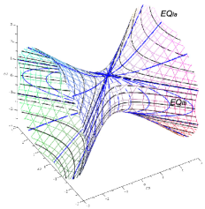
Figure 23: Equidistant systems of Type Ia ($|u_{2}|\geq R$) and Type Ib ($|u_{2}|\leq R$)

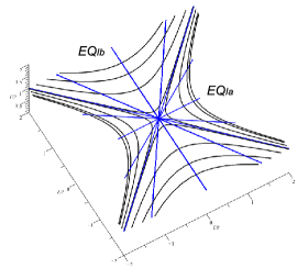
Figure 24: Projective plane for equidistant systems of Type Ia and Type Ib

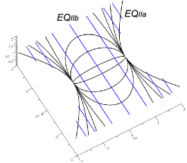
Figure 25: Projective plane for permuted equidistant systems $EQ^{*}$ of Type IIa and Type IIb

4.4 Equidistant coordinates of Type Ia and Type Ib to pseudo-polar ones

Let us fix in equidistant coordinate system of Type Ia (59) the geodesic parameter $r=\tau_{1}R$ (see Fig. 24). Then for the large $R$ angle $\tau_{1}$ tends to zero and $\tanh\tau_{1}\simeq\tau_{1}\simeq\frac{r}{R}$. In contraction limit $R\to\infty$ the Beltrami coordinates (209) transform accordingly to

$$y_{0}=R\frac{u_{0}}{u_{2}}=R\tanh\tau_{1}\cosh\tau_{2}\rightarrow t=r\cosh\tau_{2},$$

$$y_{1}=R\frac{u_{1}}{u_{2}}=R\tanh\tau_{1}\sinh\tau_{2}\rightarrow x=r\sinh\tau_{2},$$

where variables $(r,\tau_{2})$ present the pseudo-polar coordinate system that covers only part $|t|>|x|$ of pseudo-euclidean plane $E_{1,1}$ (see Fig. 24).

In case of equidistant coordinate system of Type Ib [see equation (62)] for the fixed geodesic parameter $r=\varphi R$ we get for $R^{-1}\to 0$ that $\tan\varphi\simeq\frac{r}{R}$. In contraction limit $R\to\infty$ Beltrami coordinates go into pseudo-polar ones:

$$y_{0}=R\frac{u_{0}}{u_{2}}=R\tan\varphi\sinh\tau\rightarrow\tilde{t}=r\sinh\tau,$$

$$y_{1}=R\frac{u_{1}}{u_{2}}=R\tan\varphi\cosh\tau\rightarrow\tilde{x}=r\cosh\tau.$$

and cover the remainder part $|\tilde{x}|>|\tilde{t}|$ of plane $E_{1,1}$ (see Fig. 24). For the symmetry operator we obtain $S_{EQ}^{(2)}=K_{2}^{2}\to N^{2}=X_{S}^{2}$ (see Table 3).

4.5 Equidistant coordinates of Type IIb to Cartesian ones

Let us use the equivalent form of symmetry operator $\bar{S}_{EQ}^{(2)}=K_{1}^{2}$. Two equidistant systems correspond to this operator, namely for $|u_{1}|\geq R$ and for $|u_{1}|\leq R$, which we call of Type IIa, IIb respectively (see Fig. 25). The equidistant system of Type IIb can be obtained from (62) by permutation $u_{1}\leftrightarrow u_{2}$ and it looks as follows

$$u_{0}=R\sin\varphi\sinh\tau,\quad u_{1}=R\cos\varphi,\quad u_{2}=R\sin\varphi\cosh\tau.$$ (223)

Then for the large $R$ we obtain

$$\cot\varphi=\frac{u_{1}}{\sqrt{u_{2}^{2}-u_{0}^{2}}}\simeq\frac{x}{R},\qquad\tanh\tau=\frac{u_{0}}{u_{2}}\simeq\frac{t}{R}.$$ (224)

Therefore in contraction limit $R\to\infty$ Beltrami coordinates go into Cartesian ones:

$$y_{0}=R\tanh\tau\to t,\qquad y_{1}=R\frac{\cot\varphi}{\cosh\tau}\to x.$$ (225)

For symmetry operator in the contraction limit we obtain

$$\frac{\bar{S}_{EQ}^{(2)}}{R^{2}}=\pi_{0}^{2}\to p_{0}^{2}=X_{C}^{I}.$$

As for the equidistant system of Type IIa:

$$u_{0}=R\sinh\tau_{1}\cosh\tau_{2},\quad u_{1}=R\cosh\tau_{1},\quad u_{2}=R\sinh\tau_{1}\sinh\tau_{2},$$ (226)

here we get $|y_{0}|=R|u_{0}/u_{2}|=R|\coth\tau_{2}|>R$, it means that the contraction limit $R\to\infty$ does not exist for this system of coordinates.

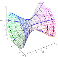
Figure 26: Pseudo-spherical system

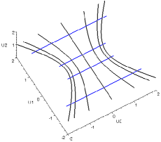
Figure 27: Projective plane for pseudo-spherical system

4.6 Pseudo-spherical coordinates to Cartesian ones

For pseudo-spherical system of coordinates (51) we have (see Fig. 27)

$$y_{0}=\frac{u_{0}}{u_{2}}=R\frac{\tanh\tau}{\sin\varphi},\qquad y_{1}=\frac{u_{1}}{u_{2}}=R\cot\varphi.$$

In limit $R\to\infty$, we obtain $\tanh\tau\simeq t/R$ and $\cot\varphi\simeq x/R$ hence the Beltrami coordinates $(y_{0},y_{1})$ go into Cartesian ones $y_{0}\to t$,   $y_{1}\to x$. In this case the symmetry operator takes the form:

$$\frac{S_{SPH}^{(2)}}{R^{2}}=\frac{L^{2}}{R^{2}}=\pi_{1}^{2}\to p_{1}^{2}=X_{C}^{I}.$$

4.7 Horicyclic coordinates to Cartesian ones

We start with horiciclyc coordinates (70) but interchange the coordinates $u_{1}\leftrightarrow u_{2}$, i.e. put (see Fig. 30)

$$u_{0}=R\frac{\tilde{x}^{2}-\tilde{y}^{2}+1}{2\tilde{y}},\qquad u_{1}=R\frac{\tilde{x}}{\tilde{y}},\qquad u_{2}=R\frac{\tilde{x}^{2}-\tilde{y}^{2}-1}{2\tilde{y}}.$$ (227)

Then the corresponding symmetry operator has the form

$$\bar{S}_{HO}^{(2)}=K_{2}^{2}-\{K_{2},L\}+L^{2}.$$ (228)

For variables $\tilde{x}$, $\tilde{y}$ we obtain

$$\tilde{x}=\frac{u_{1}}{u_{0}-u_{2}},\qquad\tilde{y}=\frac{R}{u_{0}-u_{2}}.$$ (229)

In the limit $R\to\infty$ we get $\tilde{x}\to-\frac{x}{R}$ and $\tilde{y}\to-(1+\frac{t}{R})$ and Beltrami coordinates go into Cartesian ones

$$y_{0}=R\frac{\tilde{x}^{2}-\tilde{y}^{2}+1}{\tilde{x}^{2}-\tilde{y}^{2}-1}\to t,\qquad y_{1}=2R\frac{\tilde{x}}{\tilde{x}^{2}-\tilde{y}^{2}-1}\to x.$$ (230)

For symmetry operator we have

$$\frac{\bar{S}_{HO}^{(2)}}{R^{2}}=\frac{K_{2}^{2}}{R^{2}}+\frac{1}{R}\{K_{2},\pi_{1}\}+\pi_{1}^{2}\to p_{1}^{2}=X_{C}^{I}.$$

Note that contraction for coordinates (227) is much more simple then for (70), since in this case there is no entanglement of horiciclic and Cartesian coordinates for the large $R$.

Figure 28: Horicyclic system

Figure 30: Projective plane for permuted horicyclic system $\bar{S}_{HO}$

4.8 Elliptic coordinates to elliptic I and Cartesian ones

Elliptic system (155) has three parameters $a_{1}$, $a_{2}$ and $a_{3}$, that define the position of foci on hyperboloid. On the projective plane the hyperbola foci have coordinates $F\left(0,R\sqrt{\frac{2\rho_{1}-a_{2}-a_{3}}{a_{1}-\rho_{1}}}\right)$. Then the minimal focus distance for corresponding projective hyperbolas is $|FP|=R\sqrt{\frac{a_{2}-a_{3}}{a_{1}-a_{2}}}=\frac{R}{\sinh\beta}$, or $\sinh\beta=R/|FP|=\cot\alpha$, where $\alpha$ is angle $FOP$, $|OP|=R$ (see Figs. 32 and 32). There are two interesting limiting cases in the sense of contractions. First, when the minimal focus distance $|FP|$ is fixed, so $\sinh\beta\sim R$ and second, when $\sinh\beta$ is fixed and therefore $|FP|\sim R$.

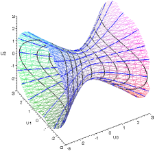
Figure 31: Elliptic system

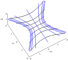
Figure 32: Projective plane for elliptic system

4.8.1 Elliptic to elliptic

Let us introduce parameter $D=\sqrt{a_{2}-a_{3}}$, which is the limit for $|FP|$ as $R\to\infty$, $a_{1}\simeq R^{2}$ and it represents the minimal focal distance to the focus point for both families of hyperbolas on $E_{1,1}$ plane.

In new variables $\xi$ and $\eta$:

$$\sinh^{2}\eta=\frac{\rho_{1}-a_{2}}{a_{2}-a_{3}},\qquad\cosh^{2}\xi=\frac{a_{2}-\rho_{2}}{a_{2}-a_{3}},$$

we can rewrite the elliptic system (155) in the form

$$u_{0} = \frac{RD}{\sqrt{a_{1}-a_{3}}}\cosh\eta\sinh\xi,$$

$$u_{1} = \frac{RD}{\sqrt{a_{1}-a_{2}}}\sinh\eta\cosh\xi,$$ (231)

$$u_{2}^{2} = R^{2}\left[1-\frac{a_{2}-a_{3}}{a_{1}-a_{2}}\sinh^{2}\eta\right]\left[1+\frac{a_{2}-a_{3}}{a_{1}-a_{3}}\sinh^{2}\xi\right].$$

In contraction limit $a_{1}\simeq R^{2}\to\infty$ and Beltrami coordinates tend into the elliptic ones of Type I (see Table 3) on $E_{1,1}$ plane:

$$y_{0}\to t=D\cosh\eta\sinh\xi,\qquad y_{1}\to x=D\sinh\eta\cosh\xi.$$

For the symmetry operator in limit $a_{1}\simeq R^{2}\to\infty$ we have

$$\frac{D^{2}}{R^{2}}\,S_{E}=\frac{D^{2}}{R^{2}}\left[L^{2}+\sinh^{2}\beta K_{2}^{2}\right]=D^{2}\pi_{1}^{2}+\frac{a_{1}-a_{2}}{R^{2}}K_{2}^{2}\to N^{2}+D^{2}p_{1}^{2}=X_{E}^{I}.$$

4.8.2 Elliptic to Cartesian

Let us fix angle $\alpha$ (or the same $\sinh\beta$) and choose for simplicity $a_{1}-a_{2}=a_{2}-a_{3}$. Then $k^{2}=k^{\prime{2}}=1/2$, $\sinh\beta=\cot\alpha=1$ and we have $S_{E}=L^{2}+K_{2}^{2}$. From equation (156) we get

$$-\mbox{cn}^{2}a=\sqrt{\left(\frac{u_{0}^{2}+u_{2}^{2}}{2R^{2}}\right)^{2}+\frac{u_{1}^{2}}{R^{2}}}-\frac{u_{0}^{2}+u_{2}^{2}}{2R^{2}},\quad-\mbox{cn}^{2}b=\sqrt{\left(\frac{u_{0}^{2}+u_{2}^{2}}{2R^{2}}\right)^{2}+\frac{u_{1}^{2}}{R^{2}}}+\frac{u_{0}^{2}+u_{2}^{2}}{2R^{2}}.$$ (232)

Taking now limit $R\to\infty$ we have

$$\mbox{cn}\,a\to\frac{ix}{R},\qquad\mbox{dn}\,b\to-\frac{it}{R},$$ (233)

and hence Beltrami coordinates (209) go into Cartesian ones : $y_{0}\to t$ and $y_{1}\to x$. For the symmetry operator we have

$$\frac{S_{E}}{R^{2}}=\pi_{1}^{2}+\frac{K_{2}^{2}}{R^{2}}\to p_{1}^{2}=X_{C}^{I}.$$

4.9 Hyperbolic coordinates to elliptic II, III, Cartesian, parabolic I and pseudo-polar ones

The hyperbolic system of coordinates (170) in algebraic form is determined by three parameters $a_{1}$, $a_{2}$ and $a_{3}$, which define the points of intersection of envelopes. On the projective plane the points have coordinates $F_{1,2}\left(\pm R\sin\alpha,0\right)$ and $G_{1,2}\left(0,\pm R\tan\alpha\right)$. Distance $|F_{1}F_{2}|$ is equal to $2f=2R\sqrt{\frac{a_{2}-a_{3}}{a_{1}-a_{3}}}=2R\sin\alpha$ (see Figs. 34 and 34). Therefore at the contraction limit $R\to\infty$ we must distinguish two cases, namely when parameter $f$ or angle $\alpha$ are fixed.

Figure 33: Hyperbolic system

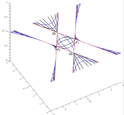
Figure 34: Projective plane for hyperbolic system

4.9.1 Hyperbolic to elliptic

We start with the case when $f\sim R/\sqrt{a_{1}}$ is fixed. Consider firstly the hyperbolic system of coordinates $H_{I}^{A}$ (when $\rho_{1}$, $\rho_{2}<a_{3}<a_{2}<a_{1}$). Introducing the new coordinates $\xi$ and $\eta$ by

$$\cosh^{2}\eta=\frac{a_{2}-\rho_{1}}{a_{2}-a_{3}},\qquad\cosh^{2}\xi=\frac{a_{2}-\rho_{2}}{a_{2}-a_{3}},$$

and taking limit $a_{1}\simeq R^{2}\to\infty$, we obtain for Beltrami coordinates (209)

$$y_{0}\to t=d\cosh\eta\cosh\xi,\qquad y_{1}\to x=d\sinh\eta\sinh\xi.$$

Here $(\xi,\eta)$ are the elliptic coordinates of Type II(i) (see Table 3) and $d=\sqrt{a_{2}-a_{3}}$ is the minimal focus distance for hyperbolas on $E_{1,1}$ plane.

In the case of hyperbolic system $H_{II}^{A}$ (when $a_{3}<\rho_{1},\rho_{2}<a_{2}<a_{1}$) using the new coordinates:

$$\cos^{2}\eta=\frac{a_{2}-\rho_{1}}{a_{2}-a_{3}},\qquad\cos^{2}\xi=\frac{a_{2}-\rho_{2}}{a_{2}-a_{3}},$$

it is easy to see that Beltrami coordinates (209) take the form of the elliptic coordinates of the Type II(ii) (see Table 3) on $E_{1,1}$ plane:

$$y_{0}\to t=d\cos\eta\cos\xi,\qquad y_{1}\to x=d\sin\eta\sin\xi,$$

where $d$ means now the maximal focus distance for ellipses. For the symmetry operator we have

$$S_{H}=K_{2}^{2}-\sin^{2}\alpha L^{2}=K_{2}^{2}-{R^{2}}\sin^{2}{\alpha}\,\pi_{1}^{2}\to N^{2}-d^{2}p_{1}^{2}=X_{E}^{II}.$$ (234)

Let us note that elliptic coordinates of Types II(i) and II(ii) do not cover completely pseudo-euclidean plane $E_{1,1}$ (see Table 3 and [33]).

4.9.2 Hyperbolic to Cartesian

Let us fix angle $\alpha$ and choose $a_{1}-a_{2}=a_{2}-a_{3}$ for the simplicity, then $\sin\alpha=1/\sqrt{2}$ and $f=R/\sqrt{2}\to\infty$, when $R\to\infty$. As one can see from Figs. 34, 34 only system $H^{A}_{II}$ on projective plane covers the origin of coordinates, therefore we proceed to contract this system with $u_{2}=R\,\mbox{dn}\,a\,\mbox{sn}\,b\geq R$. From equation (171) we obtain (considering $-\mbox{cn}^{2}b\geq\mbox{cn}^{2}a$):

$$\mbox{cn}^{2}a=\frac{u_{2}^{2}-u_{1}^{2}}{2R^{2}}-\sqrt{\left(\frac{u_{2}^{2}-u_{1}^{2}}{2R^{2}}\right)^{2}-\frac{u_{0}^{2}}{R^{2}}},\qquad-\mbox{cn}^{2}b=\frac{u_{2}^{2}-u_{1}^{2}}{2R^{2}}+\sqrt{\left(\frac{u_{2}^{2}-u_{1}^{2}}{2R^{2}}\right)^{2}-\frac{u_{0}^{2}}{R^{2}}}.$$ (235)

Therefore for the large $R$ we have

$$\mbox{cn}\,a\to\frac{t}{R},\qquad\mbox{dn}\,b\to\frac{x}{R},$$ (236)

and Beltrami coordinates contract to Cartesian ones $y_{0}\to t$ and $y_{1}\to x$. In this case the symmetry operator takes the form

$$-\frac{2}{R^{2}}S_{H}=-\frac{2}{R^{2}}\left(K_{2}^{2}-\sin^{2}\alpha L^{2}\right)=\pi_{1}^{2}-\frac{2K_{2}^{2}}{R^{2}}\to p_{1}^{2}=X_{C}^{I}.$$

4.9.3 Rotated hyperbolic to parabolic I

The principal difference between hyperbolic system and the rotated one is a position of the limit points (points of intersections of envelopes). For the rotated hyperbolic system one of the limit points is fixed in $(0,0,R)$ (see Fig. 36 and Fig. 36) and it does not depend on parameter $\alpha$ that plays the critical part for the contraction.

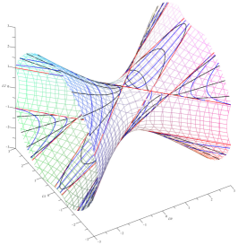
Figure 35: Rotated hyperbolic system

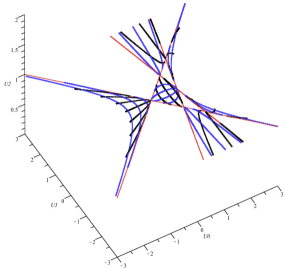
Figure 36: Projective plane for rotated hyperbolic system

Let us fix parameter $k$ (or parameter $k^{\prime}$). Then for the large $R$ we obtain

$$\mbox{sn}(a,k)\to\frac{iv}{\sqrt{kR}},\qquad\mbox{dn}(b,k^{\prime})\to iu\sqrt{\frac{k}{R}},$$ (237)

where we take into account the following expressions

$$k^{2}\mbox{sn}^{2}(a,k)=\frac{1}{2R^{2}}\left\{(u_{1}^{\prime})^{2}k^{2}-(ku_{0}^{\prime}+u_{2}^{\prime})^{2}+R^{2}\sqrt{\left[(u_{1}^{\prime})^{2}k^{2}-(ku_{0}^{\prime}+u_{2}^{\prime})^{2}+R^{2}\right]^{2}-4R^{2}k^{2}(u_{1}^{\prime})^{2}}\right\},$$

$$\mbox{dn}^{2}(b,k^{\prime})=\frac{1}{2R^{2}}\left\{(u_{1}^{\prime})^{2}k^{2}-(ku_{0}^{\prime}+u_{2}^{\prime})^{2}+R^{2}-\sqrt{\left[(u_{1}^{\prime})^{2}k^{2}-(ku_{0}^{\prime}+u_{2}^{\prime})^{2}+R^{2}\right]^{2}-4R^{2}k^{2}(u_{1}^{\prime})^{2}}\right\},$$

and $v,u$ are the parabolic coordinates (see Table 3). Here we use the coordinate system for region $H_{I}^{A}$ (with $u_{2}\geq R$, $u_{0}>0$):

$$u_{0}=R\mbox{cn}(a,k)\,i\mbox{cn}(b,k^{\prime}),\qquad u_{1}=R\,i\mbox{sn}(a,k)\,i\mbox{dn}(b,k^{\prime}),\qquad u_{2}=R\mbox{dn}(a,k)\mbox{sn}(b,k^{\prime}),$$ (238)

which after hyperbolic rotation (174) has the form:

$$u_{0}^{\prime} = \frac{R}{k^{\prime}}\left[-k\mbox{dn}(a,k)\mbox{sn}(b,k^{\prime})+i\mbox{cn}(a,k)\mbox{cn}(b,k^{\prime})\right],$$

$$u_{1}^{\prime} = R\,i\mbox{sn}(a,k)\,i\mbox{dn}(b,k^{\prime}),$$ (239)

$$u_{2}^{\prime} = \frac{R}{k^{\prime}}\left[-k\mbox{cn}(a,k)\,i\mbox{cn}(b,k^{\prime})+\mbox{dn}(a,k)\mbox{sn}(b,k^{\prime})\right].$$

Finally, in contraction limit $R\to\infty$ the rotated hyperbolic system (4.9.3) goes into the following one

$$y_{0}\to t=\frac{u^{2}+v^{2}}{2},\quad y_{1}\to x=uv,$$ (240)

which coincides with Parabolic I system of coordinates (see Table 3). For the symmetry operator we obtain ($c=k+1/k$):

$$\frac{S_{\tilde{H}}}{R}=\frac{1}{R}\left(cK_{2}^{2}+\{K_{2},L\}\right)\to\{N,p_{1}\}=X_{P}^{I}.$$

Let us note that parabolic coordinates (240) cover only part of $t>0$ and $|t|>|x|$. To describe the missing part of the pseudo-euclidean plane $t<0$ it is enough to change $u_{0}\to-u_{0}$ in rotated system (4.9.3).

4.9.4 Rotated hyperbolic to pseudo-polar

Let us take $k\sim R^{-2}$, then $k^{\prime}\sim 1$ and $c\sim R^{2}$. Using the system of coordinates (4.9.3), for the large $R$, instead of (237) we get

$$\mbox{sn}(a,k)\to i\sinh\tau_{2},\quad\mbox{cn}(b,k^{\prime})\to-i\frac{r}{R},$$ (241)

and the rotated hyperbolic system goes into pseudo-polar one

$$y_{0}\to t=r\cosh\tau_{2},\quad y_{1}\to x=r\sinh\tau_{2}.$$ (242)

For the symmetry operator we have

$$\frac{S_{\tilde{H}}}{R^{2}}=\frac{c}{R^{2}}K_{2}^{2}+\frac{1}{R^{2}}\{K_{2},L\}\to N^{2}=X_{S}^{2}.$$

Finally let us note that the interchange of coordinates $u_{1}\leftrightarrow u_{2}$ does not lead to new contractions of hyperbolic system of coordinates.

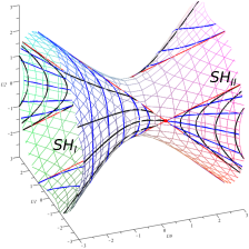
Figure 37: Semi-hyperbolic system

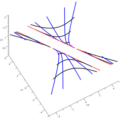
Figure 38: Projective plane for semi-hyperbolic system

4.10 Semi-hyperbolic coordinates to Cartesian, Hyperbolic I and Parabolic I ones

As we have shown in paragraph 2.4 semi-hyperbolic system of coordinates (2.4) depends on the dimensionless parameter $c=\sinh 2\beta$. It does not cover the whole surface of one-sheeted hyperboloid (see (123)). The parameter $c$, as shown in Fig. 38 and Fig. 38, splits semi-hyperbolic system of coordinates into two parts with $\sinh\tau_{1},\sinh\tau_{2}\leq c$ ($SH_{I}$) and $\sinh\tau_{1},\sinh\tau_{2}\geq c$ ($SH_{II}$).

4.10.1 Semi-hyperbolic to hyperbolic

For coordinates $\xi_{1,2}=\sinh\tau_{1,2}$ we have (assuming $\sinh\tau_{1}>\sinh\tau_{2}$)

$$\xi_{1,2}=\frac{u_{0}u_{1}}{R^{2}}+\frac{c}{2}\frac{u_{1}^{2}-u_{0}^{2}}{R^{2}}\pm\sqrt{\left\{\frac{u_{0}u_{1}}{R^{2}}+\frac{c}{2}\frac{u_{1}^{2}-u_{0}^{2}}{R^{2}}\right\}^{2}-\frac{u_{2}^{2}+2cu_{0}u_{1}}{R^{2}}}.$$ (243)

Let us take now $c=2R^{2}/l^{2}$ ($l$ is some constant). We will only consider here system $SH_{I}$ (for $SH_{II}$ angles $\tau_{1,2}\to\infty$). Equation (243) denotes the limiting procedure. Indeed we obtain $\xi_{1,2}\to\sinh\zeta_{1,2}$ as $R\to\infty$ and for Beltrmi coordinates we get

$$y_{0}\to t=\frac{l}{2}\left[\cosh\frac{\zeta_{1}-\zeta_{2}}{2}-\sinh\frac{\zeta_{1}+\zeta_{2}}{2}\right],\qquad y_{1}\to x=\frac{l}{2}\left[\cosh\frac{\zeta_{1}-\zeta_{2}}{2}+\sinh\frac{\zeta_{1}+\zeta_{2}}{2}\right],$$ (244)

i.e the semi-hyperbolic coordinate contract into hyperbolic coordinates of Type I (see Table 3). For the corresponding symmetry operator we get

$$\frac{l^{2}}{2R^{2}}S_{SH}=K_{2}^{2}+\frac{l^{2}}{2}\{\pi_{0},\pi_{1}\}\to N^{2}+l^{2}p_{0}p_{1}=X_{H}^{I}.$$

4.10.2 Semi-hyperbolic coordinates to Cartesian and Parabolic I ones

Let us fix the value of $\sinh 2\beta$. Then symmetry operator $S_{SH}$ contracts into Cartesian one

$$\frac{S_{SH}}{2R^{2}}=\frac{\sinh 2\beta}{2R^{2}}K_{2}^{2}+\frac{1}{2}\{\pi_{0},\pi_{1}\}\to p_{0}p_{1}=X_{C}^{I}.$$

In spite of this, it is easy to see that the origin of coordinates on projective plane is not covered by $SH$ system and for large $R$ the radical expression in formula (243) becomes negative (because of $u_{2}\sim R$). Hence, the semi-hyperbolic coordinates in form (2.4) do not contract to Cartesian ones on $E_{1,1}$ plane.

1. Let us consider system (2.4) but now we interchange coordinates $u_{1}\leftrightarrow u_{2}$. Then new symmetry operator is $\bar{S}_{SH}=\sinh 2\beta K_{1}^{2}-\{K_{2},L\}$. We assume that parameter $\sinh 2\beta>0$. In contraction limit $R\to\infty$ we have

$$\frac{\bar{S}_{SH}}{\sinh 2\beta R^{2}}\to\ p_{0}^{2}\simeq X_{C}^{I}.$$

Further, from equation (243), taking $u_{1}\leftrightarrow u_{2}$, we obtain for variables $\xi_{1,2}=\sinh\tau_{1,2}$:

$$\xi_{1,2}=\frac{u_{0}u_{2}}{R^{2}}+\frac{c}{2}\frac{u_{2}^{2}-u_{0}^{2}}{R^{2}}\pm\sqrt{\left\{\frac{u_{0}u_{2}}{R^{2}}+\frac{c}{2}\frac{u_{2}^{2}-u_{0}^{2}}{R^{2}}\right\}^{2}-\frac{u_{1}^{2}+2cu_{0}u_{2}}{R^{2}}}.$$ (245)

Taking limit $R\to\infty$ in (245) we get that

$$\xi_{1}\to c-\frac{c^{2}+1}{c}\frac{x^{2}}{R^{2}},\qquad\xi_{2}\to 2\frac{t}{R},$$ (246)

and hence $y_{0}\to t$ and $y_{1}\to x$, i.e. the permuted semi-hyperbolic coordinates $SH$ contract into Cartesian ones on pseudo-euclidean plane $E_{1,1}$. Note that one needs to take $SH_{I}$ or $SH_{II}$ depending on the sign of $c$ to cover the origin of coordinates on projective plane.

2. Consider now the case when $\sinh 2\beta=0$. Then in contraction limit $R\to\infty$ we have

$$-\frac{\bar{S}_{SH}}{R}=-\{K_{2},\pi_{1}\}\to\{N,p_{1}\}=X_{P}^{I},$$

which corresponds to the parabolic coordinates of Type I in $E_{1,1}$ plane. From equation (245) for the large $R$ we get

$$\xi_{1}\to\frac{u^{2}}{R},\qquad\xi_{2}\to\frac{v^{2}}{R},$$ (247)

and Beltrami coordinates go into parabolic ones of Type I (see Table 3):

$$y_{0}\to t=\frac{u^{2}+v^{2}}{2},\qquad y_{1}\to x=uv.$$

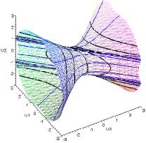
Figure 39: Elliptic-parabolic system

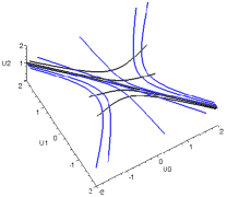
Figure 40: Projective plane for elliptic-parabolic system

4.11 Elliptic-parabolic coordinates to hyperbolic II and Cartesian ones

The elliptic-parabolic system of coordinates is determined by parameter $\gamma>0$, which is included in the definition of this system (see Fig. 40). The projective plane for this system is presented in Fig. 40.

4.11.1 Elliptic-parabolic to hyperbolic II

We consider elliptic-parabolic coordinates (136) with parameter $\gamma\sim R^{2}/l^{2}$ ($l>0$ is some constant) and put $\xi_{1}=-\gamma/\sinh^{2}\tau_{2}$ and $\xi_{2}=\gamma/\cosh^{2}\tau_{1}$. From equation (136) we have ($\xi_{1}<0<\xi_{2}\leq\gamma$):

$$\xi_{1,2}=-\frac{1}{2R^{2}}\left\{(u_{0}-u_{1})^{2}+\gamma(u_{0}^{2}-u_{1}^{2})\pm\sqrt{\left[(u_{0}-u_{1})^{2}+\gamma(u_{0}^{2}-u_{1}^{2})\right]^{2}+4R^{2}\gamma(u_{0}-u_{1})^{2}}\right\}.$$ (248)

Then in contraction limit we obtain

$$\xi_{1,2}\to\mp 2e^{2\zeta_{1,2}},$$ (249)

and for Beltrami coordinates we have ($t>x$)

$$y_{0}\to t=l\left[\sinh(\zeta_{2}-\zeta_{1})+e^{\zeta_{1}+\zeta_{2}}\right],\qquad y_{1}\to x=l\left[\sinh(\zeta_{2}-\zeta_{1})-e^{\zeta_{1}+\zeta_{2}}\right].$$ (250)

where $\zeta_{1}$ and $\zeta_{2}$ are the hyperbolic coordinates of Type II (see Table 3). For symmetry operator in the same limit we have

$$\frac{l^{2}}{R^{2}}S_{EP}=\frac{l^{2}}{R^{2}}\left[\gamma K_{2}^{2}+(K_{1}+L)^{2}\right]=K_{2}^{2}+l^{2}(\pi_{0}+\pi_{1})^{2}\to N^{2}+l^{2}(p_{0}+p_{1})^{2}=X_{H}^{II}.$$

4.11.2 Elliptic-parabolic to Cartesian

We will start from coordinates (136) but we will interchange coordinates $u_{1}\leftrightarrow u_{2}$. Then we have

$$\bar{S}_{EP}=\gamma K_{1}^{2}+(K_{2}-L)^{2}.$$ (251)

Let us fix parameter $\gamma>0$. Introducing the new variables by $\xi_{1}=\cosh\tau_{1}$, $\xi_{2}=\sinh\tau_{2}$ and using equation (136) it is easy to find that (we consider $u_{2}>u_{0}$, $\tau_{2}<0$ to cover the origin of coordinates):

$$\xi^{2}_{1,2}=\frac{\pm u_{0}(\gamma+1)\pm u_{2}(\gamma-1)-\sqrt{\left[u_{0}(\gamma+1)+u_{2}(\gamma-1)\right]^{2}+4R^{2}\gamma}}{2(u_{0}-u_{2})}.$$ (252)

From formula (252) we have for the large $R$

$$\sinh\tau_{1}\to\sqrt{\frac{\gamma}{\gamma+1}}\frac{x}{R},\qquad\sinh\tau_{2}\to-\sqrt{\gamma}\left(1+\frac{t}{R}\right),$$ (253)

and Beltrami coordinates go to Cartesian ones: $y_{0}\to t$ and $y_{1}\to-x$. For symmetry operator $\bar{S}_{EP}$ we get

$$\frac{\bar{S}_{EP}}{R^{2}}=\gamma\pi_{0}^{2}+\left(\frac{K_{2}}{R}+\pi_{1}\right)^{2}\to\gamma p_{0}^{2}+p_{1}^{2}\simeq X_{C}^{I}.$$

Finally let us note that we do not use the elliptic-parabolic system of coordinates in form (136) because for the large $R$ the variables $\xi_{1}=\cosh\tau_{1}$ and $\xi_{2}=\sinh\tau_{2}$ are expressed as the combination of Cartesian coordinates $t$ and $x$.

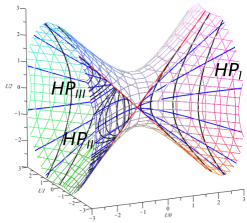
Figure 41: Hyperbolic-parabolic system

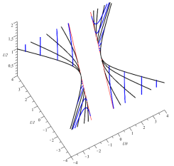
Figure 42: Projective plane for hyperbolic-parabolic system

4.12 Hyperbolic-parabolic to hyperbolic III, Cartesian and Parabolic I

The hyperbolic-parabolic system of coordinates depends on parameter $\gamma>0$. This parameter defines the points of intersection of envelopes (146) on hyperboloid with coordinates $\left(\pm R\frac{1-\gamma}{2\sqrt{\gamma}},\pm R\frac{1+\gamma}{2\sqrt{\gamma}},0\right)$ (see Fig. 42).

4.12.1 Hyperbolic-parabolic to Hyperbolic III

In this section we shall always assume that $\gamma=R^{2}/l^{2}$ ($l$ is some constant). We introduce notation $\xi_{1}=\sin\theta$ and $\xi_{2}=\sin\phi$. Then, for the coordinates of Type I (143) we obtain

$$\xi^{2}_{1,2}=\frac{u_{0}(1-\gamma)-u_{1}(\gamma+1)\mp\sqrt{(u_{0}(1-\gamma)-u_{1}(1+\gamma))^{2}-4l^{2}}}{2(u_{0}-u_{1})}$$ (254)

whereas for coordinates of Type II (2.7)

$$\xi^{2}_{1,2}=\frac{u_{0}-u_{1}}{2R^{2}\gamma}\left\{u_{0}(1-\gamma)-u_{1}(\gamma+1)\pm\sqrt{\left[u_{0}(1-\gamma)-u_{1}(1+\gamma)\right]^{2}-4l^{2}}\right\}.$$ (255)

Let us put now $\xi^{-1}_{1,2}=\frac{\sqrt{2}l}{R}e^{\zeta_{2,1}}$ for coordinates of Type I and ${\xi_{1,2}}=\frac{\sqrt{2}l}{R}e^{\zeta_{2,1}}$ for Type II respectively. It is easy to see that in contraction limit $R\to\infty$ Beltrami coordinates $y_{0}$ and $y_{1}$ of the system of Type I, II contract into hyperbolic coordinates of Type III, that cover part $x>t$ on pseudo-euclidean plane $E_{1,1}$ (see Table 3):

$$y_{0}\to t=l\left[\cosh(\zeta_{1}-\zeta_{2})-e^{\zeta_{1}+\zeta_{2}}\right],\qquad y_{1}\to x=l\left[\cosh(\zeta_{1}-\zeta_{2})+e^{\zeta_{1}+\zeta_{2}}\right].$$ (256)

For hyperbolic-parabolic coordinates (2.7) of Type III we obtain

$$\xi^{2}_{1,2}=\frac{u_{0}-u_{1}}{2R^{2}\gamma}\left\{u_{0}(\gamma-1)+u_{1}(\gamma+1)\pm\sqrt{\left[u_{0}(\gamma-1)+u_{1}(1+\gamma)\right]^{2}-4R^{2}\gamma}\right\}$$ (257)

here we use notation $\xi_{1}=\sinh\theta$ and $\xi_{2}=\sinh\phi$. Choosing now ${\xi_{1,2}}=\frac{\sqrt{2}l}{R}e^{\zeta_{1,2}}$ we get that in contraction limit $R\to\infty$ the system of Type III contracts into hyperbolic coordinates of Type III that cover part $t>x$ on pseudo-euclidean plane $E_{1,1}$ (see Table 3):

$$y_{0}\to t=l\left[\cosh(\zeta_{1}-\zeta_{2})+e^{\zeta_{1}+\zeta_{2}}\right],\qquad y_{1}\to x=l\left[\cosh(\zeta_{1}-\zeta_{2})-e^{\zeta_{1}+\zeta_{2}}\right].$$ (258)

For the corresponding symmetry operator in the same limit we get

$$-\frac{l^{2}}{R^{2}}S_{HP}=K_{2}^{2}-\frac{l^{2}}{R^{2}}(K_{1}+L)^{2}\to N^{2}-l^{2}(p_{0}+p_{1})^{2}=X_{H}^{III}.$$

Let us note that there is uncovered part of pseudo-Euclidean plane, namely $|t+x|<2|l|$. This result is a consequence of splitting the hyperbolic-parabolic coordinates as shown in Fig. 42.

4.12.2 Hyperbolic-parabolic to Cartesian

As in the previous section, we look at all three types of hyperbolic-parabolic coordinates but interchange coordinates $u_{1}\leftrightarrow u_{2}$. Then we arrive to the equivalent symmetry operator $\bar{S}_{HP}=-\gamma K_{1}^{2}+(K_{2}-L)^{2}$, where $\gamma>0$ and $\gamma\neq 1$ (this case is considered later). In contraction limit $R\to\infty$ we have

$$\frac{\bar{S}_{HP}}{R^{2}}=-\gamma\pi_{0}^{2}+\left(\frac{K_{2}}{R}+\pi_{1}\right)^{2}\to-\gamma p_{0}^{2}+p_{1}^{2}\simeq X_{C}^{I}.$$

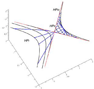
Figure 43: Projective plane for permuted system $\bar{S}_{HP}$, $0<\gamma<1$

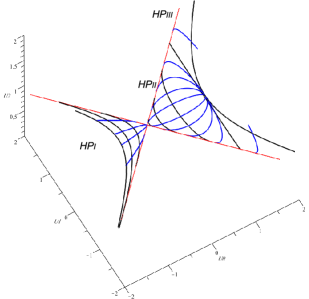
Figure 44: Projective plane for permuted system $\bar{S}_{HP}$, $\gamma>1$

The point of intersection of envelopes on projective plane is in $\left(\frac{1-\gamma}{1+\gamma},0\right)$. Therefore the origin of coordinates is covered by different types of $HP$ system, depending on the value of $\gamma$.

From relations (254) for $HP_{I}$, after interchanging $u_{1}\leftrightarrow u_{2}$ we obtain

$$\xi^{2}_{1,2}=\frac{u_{0}(1-\gamma)-u_{2}(\gamma+1)\mp\sqrt{\left[u_{0}(1-\gamma)-u_{2}(\gamma+1)\right]^{2}-4R^{2}\gamma}}{2(u_{0}-u_{2})}$$ (259)

and hence, for the large $R$

$$\cos\theta\to\sqrt{\frac{\gamma}{1-\gamma}}\frac{x}{R},\qquad\sin\phi\to\sqrt{\gamma}\left(1+\frac{t}{R}\right).$$ (260)

Here we take $0<\gamma<1$, because only in this case system $HP_{I}$ on the projective plane covers the origin $(0,0)$ and goes to Cartesian coordinates (see Fig. 44 with $\gamma=1/2$).

In the same way for permuted system $HP_{II}$ from (255) we find

$$\xi^{2}_{1,2}=\frac{u_{0}-u_{2}}{2\gamma R^{2}}\left\{u_{0}(1-\gamma)-u_{2}(\gamma+1)\pm\sqrt{\left[u_{0}(1-\gamma)-u_{2}(\gamma+1)\right]^{2}-4\gamma R^{2}}\right\}$$ (261)

and for the large $R$

$$\sin\theta\to\frac{1}{\sqrt{\gamma}}\left(1-\frac{t}{R}\right),\qquad\cos\phi\to\sqrt{\frac{\gamma}{\gamma-1}}\frac{x}{R},$$ (262)

where now $\gamma>1$, because only in this case permuted system $HP_{II}$ on the projective plane covers the origin $(0,0)$ and contracts to Cartesian system (see Fig. 44 with $\gamma=2$).

The permuted system obtained from $HP_{III}$ does not cover $(0,0)$ for any value of $\gamma$ and in contraction limit does not contract to Cartesian coordinates.

4.12.3 Hyperbolic-parabolic to Parabolic I

We will consider here the case when parameter $\gamma=1$. In this case the point of intersection of envelopes is in $(0,0)$ of projective plane and $HP$ systems do not cover this point.

For symmetry operator we obtain

$$\bar{S}_{HP}=-K_{1}^{2}+(K_{2}-L)^{2}=2K_{2}^{2}-\{K_{2},L\}-R^{2}\Delta_{LB}$$

and in contraction limit $R\to\infty$ we get

$$-\frac{\bar{S}_{HP}}{R}-R\Delta_{LB}=-2\frac{K_{2}^{2}}{R}-\{K_{2},\pi_{1}\}\to\{N,p_{1}\}=X_{P}^{I}.$$

For coordinates $\xi_{1,2}^{2}=\left(-u_{2}\mp\sqrt{u_{2}^{2}-R^{2}}\right)/{(u_{0}-u_{2})}$ of Type I (259) we have:

$$\xi_{1}^{2}\to 1-\frac{u^{2}}{R},\qquad\xi_{2}^{2}\to 1-\frac{v^{2}}{R};$$ (263)

for coordinates $\xi_{1,2}^{2}=(u_{0}-u_{2})\left(-u_{2}\pm\sqrt{u_{2}^{2}-R^{2}}\right)/R^{2}$ of Type II (261) we obtain

$$\xi_{1}^{2}\to 1-\frac{v^{2}}{R},\qquad\xi_{2}^{2}\to 1-\frac{u^{2}}{R};$$ (264)

and for coordinates $\xi_{1,2}^{2}=(u_{0}-u_{2})\left(u_{2}\pm\sqrt{u_{2}^{2}-R^{2}}\right)/R^{2}$ of Type III (here $\xi_{1}=\sinh\theta$, $\xi_{2}=\sinh\phi$) we get

$$\xi_{1}^{2}\to 1+\frac{v^{2}}{R},\qquad\xi_{2}^{2}\to 1+\frac{u^{2}}{R}.$$ (265)

In limit $R\to\infty$ we obtain

$$y_{0}\to t=\frac{1}{2}\left(u^{2}+v^{2}\right),\qquad y_{1}\to x=uv,$$

which coincides with Parabolic I coordinates in pseudo-euclidean plane $E_{1,1}$ (see Table 3).

Figure 45: Semi-circular-parabolic system

Figure 46: Projective plane for semi-circular-parabolic system

4.13 Semi-circular-parabolic to Cartesian

In contraction limit operator $S_{SCP}$ gives

$$\frac{S_{SCP}}{R}=\frac{1}{R}\{K_{1},K_{2}\}+\frac{1}{R}\{K_{2},L\}\to\left\{p_{0},N\right\}+\left\{p_{1},N\right\},$$ (266)

which was already well known as the operator that does not generate a coordinate system with separation of variables (see [33]). The contraction limit of SCP system also does not correspond to any separable system on $E_{1,1}$.

Nevertheless, it is possible to construct the equivalent form of semi-circular-parabolic system which contracts to Cartesian coordinates. Let us make two consecutive hyperbolic rotations. The first one through the angle $a_{1}\not=0$ with respect to axis $u_{1}$ and the second one through angle $a_{2}\not=0$ with respect to axis $u_{2}$. The resulting rotation is given by matrix

$$\left({{\begin{array}[]{*{20}c}u^{\prime}_{0}\\ u^{\prime}_{1}\\ u^{\prime}_{2}\end{array}}}\right)=\left({{\begin{array}[]{*{20}c}\cosh a_{2}\cosh a_{1}&\sinh a_{2}&\cosh a_{2}\sinh a_{1}\\ \sinh a_{2}\cosh a_{1}&\cosh a_{2}&\sinh a_{2}\sinh a_{1}\\ \sinh a_{1}&0&\cosh a_{1}\end{array}}}\right)\left({{\begin{array}[]{*{20}c}u_{0}\\ u_{1}\\ u_{2}\end{array}}}\right).$$ (267)

To simplify all subsequent formulas we choose $a_{1}=\ln\frac{1}{\sqrt{2}}$ and $a_{2}=-\tanh^{-1}(\cosh a_{1}+\sinh a_{1})=-\tanh^{-1}\frac{1}{\sqrt{2}}$. Then the new symmetry operator takes the form

$$\tilde{S}_{SCP}=\frac{1}{4}K_{1}^{2}+\frac{1}{4}\left\{K_{1},K_{2}\right\}-\frac{3}{4}K_{2}^{2}+\frac{1}{\sqrt{2}}\left\{K_{2},L\right\}-\frac{1}{2}L^{2}.$$ (268)

In contraction limit $R\to\infty$ we obtain

$$\frac{4}{R^{2}}\left(\frac{R^{2}}{2}\Delta_{LB}-\tilde{S}_{SCP}\right)\to p_{0}^{2}=X_{C}^{I}.$$ (269)

For coordinates $\xi$ and $\eta$, after some long and tedious calculations we get

$$\xi\to 2\left(1+\frac{x}{R}\right),\qquad\eta\to\sqrt{2}-\frac{2t}{R},$$ (270)

and Beltrami coordinates (209) contract into the Cartesian ones: $y_{0}\to t$, $y_{1}\to x$.

5 Conclusion and Discussion

From the algebraic point of view on the problem of variables separation for the two-dimensional Helmholtz equation the set of the first and second order operators have been constructed. These operators do not commute between themselves, but they commute with Laplace-Beltrami operator and correspond to separation of variables in Helmholtz equation on two-dimensional hyperboloid embedded in three-dimensional Minkovski space $E_{2,1}$. The results of the classification of second order operators are essentially in agreement with those of [85]. We have shown that the procedure of the construction of separable systems of coordinates, based on the first order operator is not unique and leads not only to the orthogonal subgroup type coordinates but describes also nonorthogonal ones. We have found three such type systems of coordinates. The detailed description of all possible orthogonal systems of coordinates, corresponding to each operator sets $\left\{\Delta_{LB},S^{(2)}_{\alpha}\right\}$ is given as for two-sheeted (upper sheet) $H_{2}$, either for one-sheeted ${\tilde{H}}_{2}$ hyperboloids.

All coordinate systems on $H_{2}$ parametrize completely the surface of hyperboloid. As a consequence there exists an intimate connection between symmetry operators and systems of coordinates at the contraction limit from two-sheeted hyperboloid into euclidean plane $E_{2}$. All coordinate systems in Euclidean plane $E_{2}$ can be obtained as the limit of space $H_{2}$ under the contraction procedure $R\to\infty$. We have presented here some new contractions that were unnoticed in the previous papers [29, 67] in addition to already known ones. The contraction of the nonorthogonal systems of coordinates on $H_{2}$ into $E_{2}$ ones also are given.

We have shown that differently from $H_{2}$ hyperboloid, only five, namely: pseudo-spherical, equidistant (splitting into two parts), horiciclic, elliptic-parabolic and elliptic systems of coordinates completely cover one-sheeted hyperboloid. As a reflection of this fact, the contraction limit of symmetry operator does not guarantee the existence of the contractions of the corresponding system of coordinates on ${\tilde{H}}_{2}$ hyperboloid into the pseudo-euclidean plane $E_{1,1}$. It occurs with the semi-circular-parabolic, semi-hyperbolic and hyperbolic coordinate systems. Nevertheless, one can consider the contraction limit $R\to\infty$ in these coordinates using the complex ones. We can explain this situation by example of semi-circular-parabolic system of coordinates. Let us consider operator $\bar{S}_{SCP}$

$$\bar{S}_{SCP}=\{K_{1},K_{2}\}-\{K_{1},L\},$$

which corresponds to semi-circular-parabolic system (129) with permutation $u_{1}\leftrightarrow u_{2}$. For limit $R\to\infty$ it is easy to see that it contracts into Cartesian operator on $E_{1,1}$:

$$-\frac{\bar{S}_{SCP}}{2R^{2}}=-\frac{1}{2R}\{\pi_{0},N\}+\frac{1}{2}\{\pi_{0},\pi_{1}\}\to p_{0}p_{1}=X_{C}^{I}.$$

Now we are going to check what happens to the semi-circular-parabolic system at the contraction limit $R\to\infty$. Let us consider system (128) wherein previously we make the change $u_{1}\leftrightarrow u_{2}$. The result is

$$\lambda_{1}+\lambda_{2}=2u_{1}(u_{2}-u_{0}),\qquad\lambda_{1}\lambda_{2}=R^{2}(u_{2}-u_{0})^{2},$$ (271)

that gives three possibilities for the values of $\lambda_{i}$: 1. $\lambda_{i}\geqslant 0$; 2. $\lambda_{i}\leqslant 0$; 3. $\lambda_{1}=a+ib$, $\lambda_{2}=a-ib$, $a,b\in\mathbb{R}$. For the first and the second ones the coordinate system covers only the part of hyperboloid when $|u_{1}|\geqslant R$, because in these cases

$$u_{1}^{2}=R^{2}\frac{\left(\lambda_{1}+\lambda_{2}\right)^{2}}{4\lambda_{1}\lambda_{2}}\geqslant R^{2}.$$ (272)

Geometrically in contraction limit $R\to\infty$ the coordinate grid for permuted SCP system on the projective plane results to be empty. To avoid it let us formally consider the third case with $a=AR^{2}$, $b=BR^{2}$, $A\in\mathbb{R}$, $B>0$.

Then coordinate system (nonorthogonal and non separable) looks as follows ($|u_{1}|<R$ and we consider $u_{2}>0$):

$$u_{0} = \frac{R}{2}\left(\sqrt{A^{2}+B^{2}}-\frac{B^{2}}{\left(A^{2}+B^{2}\right)^{3/2}}\right),$$

$$u_{1} = R\frac{A}{\sqrt{A^{2}+B^{2}}},$$ (273)

$$u_{2} = \frac{R}{2}\left(\sqrt{A^{2}+B^{2}}+\frac{B^{2}}{\left(A^{2}+B^{2}\right)^{3/2}}\right).$$

For the above system variables $A$ and $B$ contract in such a way

$$A=\frac{u_{1}(u_{0}+u_{2})}{R^{2}}\to-\frac{x}{R},\qquad B=\frac{u_{0}+u_{2}}{R}\sqrt{1-\frac{u_{1}^{2}}{R^{2}}}\to 1+\frac{t}{R}$$ (274)

and finally one obtains Cartesian coordinates $y_{0}\to t$, $y_{1}\to x$.

Thus we have investigated all forms of real analytic contractions from one-sheeted hyperboloid ${\tilde{H}}_{2}$ including the equivalent systems of coordinates. Some of them (equivalent systems of coordinates), as equidistant ones, give us different contraction limits on $E_{1,1}$. We have also considered the contraction of the nonorthogonal systems of coordinates on ${\tilde{H}}_{2}$ and have shown that they transform into nonorthogonal ones on $E_{1,1}$ classified earlier by Kalnins in [33].

We shed the light on the mysterious existence of an invariant operator (266) which does not correspond to any separation system of coordinates for the Helmholtz equation on pseudo-euclidean space $E_{1,1}$. We have observed that the relation between symmetry operators and separation systems of coordinates on the euclidean or pseudo-euclidean spaces can sometimes be better understood in the framework of contractions of the spaces of constant curvature as spheres or hyperboloids into these ”flat” spaces.

We have shown that except one, namely parabolic coordinates of type II, all orthogonal systems of coordinates on pseudo-euclidean plane $E_{1,1}$ could be obtained by contraction limit $R\to\infty$ from a system on the one-sheeted hyperboloid ${\tilde{H}}_{2}$.

To find the counterpart of parabolic coordinates of type II on ${\tilde{H}}_{2}$ hyperboloid, which we have not found among the nine orthogonal systems of coordinates, let us make the following steps. Let us consider formula (72) describing the general form of operator $S^{(2)}$, choosing in (72) $b=e=1$, $c=0$ and $a=f=-d=\frac{\alpha}{R}$, where $\alpha$ is a constant. Then we obtain the ”minimal” operator

$$S^{(2)}=\{K_{1},K_{2}\}+\{L,K_{2}\}+\frac{\alpha}{R}\left(L-K_{1}\right)^{2}$$ (275)

which contracts into $X_{P}^{II}$:

$$\frac{S^{(2)}}{R}\to\{p_{0},N\}+\{p_{1},N\}+\alpha(p_{0}-p_{1})^{2}=X_{P}^{II}.$$ (276)

The characteristic equation (116) corresponding to operator (275) gives the solution

$$\lambda_{1}+\lambda_{2}=\frac{\alpha}{R}\left(u_{0}+u_{1}\right)^{2}+2u_{2}\left(u_{0}-u_{1}\right),\quad\frac{\lambda_{1}\lambda_{2}}{R^{2}}=(u_{0}-u_{1})^{2}-\frac{4\alpha}{R}u_{2}(u_{0}+u_{1}).$$ (277)

Since we are interested in contractions only, we consider the transition for large $R$ directly for system of equations (277). From (277) it is easy to see that

$$\frac{\lambda_{1}+\lambda_{2}}{R}\simeq 2(t-x),\qquad\frac{\lambda_{1}\lambda_{2}}{R^{2}}\simeq(t-x)^{2}-4\alpha(t+x),$$ (278)

where $(t,x)$ are Cartesian coordinates on $E_{1,1}$. Introducing new variables $\xi=-\lambda_{1}/(4R)$ and $\eta=-\lambda_{2}/(4R)$ and expressing $t$, $x$, from the above system we obtain the parabolic coordinates of type II

$$t=\frac{1}{2\alpha}\left(\eta-\xi\right)^{2}-\left(\eta+\xi\right),\qquad x=\frac{1}{2\alpha}\left(\eta-\xi\right)^{2}+\left(\eta+\xi\right).$$ (279)

Thus, the contractions to the parabolic coordinates of type II can also be found within a compound system of coordinates on one-sheeted hyperboloid corresponding to symmetry operator (275).

In the nearest future we are planning to continue our investigation on the contractions of basis functions and interbases expansions associated with orthogonal separation systems of coordinates for Helmholtz equation on one- and two-sheeted hyperboloids.

6 Acknowledgments

Authors thank E. Kalnis for the useful discussion on the subject of this article. The research by G.S. Pogosyan was partially supported by the Armenian national grant 13-1C288 and the Armenian-Belarus grant Nr. 13RB-035. We appreciate the program PRO-SNI 2015 (UdeG).

Table 1: Coordinate Systems on the Two-sheeted Hyperboloid (^∗ means permutation $u_{1}\leftrightarrow u_{2}$)

Coordinate System, Operator	Coordinates	Contracted System on $E_{2}$
$\begin{array}[]{ll}\text{Ia.~{}(pseudo)-Spherical (SPH)}\\ L^{2}\\ \tau>0,0\leqslant\varphi<2\pi\end{array}$	$\begin{array}[]{ll}u_{0}=R\cosh\tau\\ u_{1}=R\sinh\tau\cos\varphi\\ u_{2}=R\sinh\tau\sin\varphi\end{array}$	Polar
$\begin{array}[]{ll}\text{Ib.~{}Spherical (}\mathit{nonorthogonal}\text{)}\\ L\\ \tau>0,0\leqslant\varphi<2\pi\end{array}$	$\begin{array}[]{ll}u_{0}=R\cosh\tau\\ u_{1}=R\sinh\tau\cos(\varphi+R\tau/\alpha)\\ u_{2}=R\sinh\tau\sin(\varphi+R\tau/\alpha)\end{array}$	Polar nonorthogonal
$\begin{array}[]{ll}\text{IIa.~{}Equidistant (EQ)}\\ K_{2}^{2}\\ \tau_{1},\tau_{2}\in\mathbb{R}\end{array}$	$\begin{array}[]{ll}u_{0}=R\cosh\tau_{1}\cosh\tau_{2}\\ u_{1}=R\cosh\tau_{1}\sinh\tau_{2}\\ u_{2}=R\sinh\tau_{1}\end{array}$	Cartesian
$\begin{array}[]{ll}\text{IIb.~{}Equidistant (}\mathit{nonorthogonal}\text{)}\\ K_{2}\\ \tau_{1},\tau_{2}\in\mathbb{R}\end{array}$	$\begin{array}[]{ll}u_{0}=R\cosh\tau_{1}\cosh(\tau_{2}+R\tau_{1}/\alpha)\\ u_{1}=R\cosh\tau_{1}\sinh(\tau_{2}+R\tau_{1}/\alpha)\\ u_{2}=R\sinh\tau_{1}\end{array}$	Cartesian nonorthogonal
$\begin{array}[]{ll}\text{IIIa.~{}Horicyclic (HO)}\\ (K_{1}+L)^{2}\\ \tilde{x}\in\mathbb{R},\tilde{y}>0\end{array}$	$\begin{array}[]{ll}u_{0}=R\frac{\tilde{x}^{2}+\tilde{y}^{2}+1}{2\tilde{y}}\vspace{1mm}\\ u_{1}=R\frac{\tilde{x}^{2}+\tilde{y}^{2}-1}{2\tilde{y}}\vspace{1mm}\\ u_{2}=R\frac{\tilde{x}}{\tilde{y}}\end{array}$	Cartesian
$\begin{array}[]{ll}\text{IIIb.~{}Horicyclic}^{*}\text{(}\mathit{nonorthogonal}\text{)}\\ K_{2}-L\\ \tilde{x}\in\mathbb{R},\tilde{y}>0\end{array}$	$\begin{array}[]{ll}u_{0}=R\frac{\left(\tilde{x}+\tilde{y}-1\right)^{2}+\tilde{y}^{2}+1}{2\tilde{y}}\vspace{1mm}\\ u_{1}=R\frac{\tilde{x}+\tilde{y}-1}{\tilde{y}}\vspace{1mm}\\ u_{2}=R\frac{\left(\tilde{x}+\tilde{y}-1\right)^{2}+\tilde{y}^{2}-1}{2\tilde{y}}\end{array}$	Cartesian nonorthogonal
$\begin{array}[]{ll}\text{IV.~{}Elliptic-Parabolic (EP)}\\ (K_{1}+L)^{2}+\gamma K_{2}^{2},\gamma>0\\ a\geq 0,\theta\in\left(-\frac{\pi}{2},\frac{\pi}{2}\right)\end{array}$	$\begin{array}[]{ll}u_{0}=\frac{R}{\sqrt{\gamma}}\frac{\cosh^{2}a-\sin^{2}\theta+\gamma}{2\cos\theta\cosh a}\vspace{1mm}\\ u_{1}=\frac{R}{\sqrt{\gamma}}\frac{\cosh^{2}a-\sin^{2}\theta-\gamma}{2\cos\theta\cosh a}\vspace{1mm}\\ u_{2}=R\tan\theta\tanh a\end{array}$	$\begin{array}[]{ll}\text{Cartesian }(\gamma\neq 1)\\ \hdashline\\ \text{Parabolic }(\gamma=1)\end{array}$
$\begin{array}[]{ll}\text{V.~{}Hyperbolic-Parabolic (HP)}\\ (K_{1}+L)^{2}-\gamma K_{2}^{2},\gamma>0\\ b>0,\theta\in\left(0,\pi\right)\end{array}$	$\begin{array}[]{ll}u_{0}=\frac{R}{\sqrt{\gamma}}\frac{\cosh^{2}b-\sin^{2}\theta+\gamma}{2\sin\theta\sinh b}\vspace{1mm}\\ u_{1}=\frac{R}{\sqrt{\gamma}}\frac{\cosh^{2}b-\sin^{2}\theta-\gamma}{2\sin\theta\sinh b}\vspace{1mm}\\ u_{2}=R\cot\theta\coth b\end{array}$	Cartesian
$\begin{array}[]{ll}\text{VIa.~{}Semi-Circular-Parabolic (SCP)}\\ \{K_{1},K_{2}\}+\{K_{2},L\}\\ \xi,\eta>0\end{array}$	$\begin{array}[]{ll}u_{0}=R\frac{\left(\eta^{2}+\xi^{2}\right)^{2}+4}{8\xi\eta}\vspace{1mm}\\ u_{1}=R\frac{\left(\eta^{2}+\xi^{2}\right)^{2}-4}{8\xi\eta}\vspace{1mm}\\ u_{2}=R{\frac{{\eta}^{2}-{\xi}^{2}}{2\xi\eta}}\end{array}$	Cartesian

Coordinate System, Operator	Coordinates	Contracted System on $E_{2}$
$\begin{array}[]{ll}\text{VIb.~{}Semi-Circular-Parabolic (SCP')}\\ K_{2}^{2}-K_{1}^{2}-\{K_{1},L\}/\sqrt{2}+\{K_{2},L\}/\sqrt{2}\\ \xi,\eta>0\end{array}$	$\begin{array}[]{ll}u_{0}=R\frac{\left(\eta^{2}+\xi^{2}\right)^{2}+4}{8\xi\eta}\vspace{1mm}\\ u_{1}+u_{2}=R\frac{{\eta}^{2}-{\xi}^{2}}{\sqrt{2}\xi\eta}\vspace{1mm}\\ u_{1}-u_{2}=R\frac{\left(\eta^{2}+\xi^{2}\right)^{2}-4}{4\sqrt{2}\xi\eta}\end{array}$	Cartesian
$\begin{array}[]{ll}\text{VIIa.~{}Elliptic (E)}\\ L^{2}+\sinh^{2}\beta K_{2}^{2},\ \sinh^{2}\beta=\frac{a_{1}-a_{2}}{a_{2}-a_{3}}\\ a_{3}<a_{2}\leq\rho_{2}<a_{1}\leq\rho_{1},\ k^{2}=\frac{a_{2}-a_{3}}{a_{1}-a_{3}},\\ a\in\left(iK^{\prime},iK^{\prime}+2K\right),b\in\left[0,4K^{\prime}\right)\end{array}$	$\begin{array}[]{ll}u_{0}^{2}=R^{2}{\frac{\left({\rho_{1}}-{a_{3}}\right)\left({\rho_{2}}-{a_{3}}\right)}{\left({a_{1}}-{a_{3}}\right)\left({a_{2}}-{a_{3}}\right)}\vspace{2mm}}\\ u_{1}^{2}=R^{2}{\frac{\left({\rho_{1}}-{a_{2}}\right)\left({\rho_{2}}-{a_{2}}\right)}{\left({a_{1}}-{a_{2}}\right)\left({a_{2}}-{a_{3}}\right)}\vspace{2mm}}\\ u_{2}^{2}=R^{2}{\frac{\left({\rho_{1}}-{a_{1}}\right)\left(a_{1}-\rho_{2}\right)}{\left({a_{1}}-{a_{2}}\right)\left({a_{1}}-{a_{3}}\right)}}\end{array}$ $\begin{array}[]{ll}u_{0}=R\mbox{sn}(a,k)\mbox{dn}(b,k^{\prime})\vspace{2mm}\\ u_{1}=iR\mbox{cn}(a,k)\mbox{cn}(b,k^{\prime})\vspace{2mm}\\ u_{2}=iR\mbox{dn}(a,k)\mbox{sn}(b,k^{\prime})\end{array}$	$\begin{array}[]{ll}\text{Elliptic}\\ (a_{1}-a_{2}=D^{2},-a_{3}\simeq R^{2})\\ \hdashline\text{Polar}\\ (a_{1}-a_{2}\simeq R^{-2},a_{2}-a_{3}\simeq R^{2})\\ \hdashline\text{Cartesian}\\ (a_{1}-a_{2}=a_{2}-a_{3})\end{array}$
$\begin{array}[]{ll}\text{VIIb.~{}Elliptic (\~{E}) (h. rotation of E)}\\ \cosh 2\beta L^{2}+1/2\sinh 2\beta\{K_{1},L\}\\ \end{array}$	$\begin{array}[]{ll}u_{0}=\frac{R}{k}\left\{\mbox{sn}(a,k)\mbox{dn}(b,k^{\prime})+ik^{\prime}\mbox{cn}(a,k)\mbox{cn}(b,k^{\prime})\right\}\vspace{2mm}\\ u_{1}=\frac{R}{k}\left\{k^{\prime}\mbox{sn}(a,k)\mbox{dn}(b,k^{\prime})+i\mbox{cn}(a,k)\mbox{cn}(b,k^{\prime})\right\}\vspace{2mm}\\ u_{2}=iR\mbox{dn}(a,k)\mbox{sn}(b,k^{\prime})\end{array}$	Parabolic
$\begin{array}[]{ll}\text{VIII.~{}Hyperbolic (H)}\\ K_{2}^{2}-\sin^{2}\alpha\>L^{2}\\ \sin^{2}\alpha=\frac{a_{2}-a_{3}}{a_{1}-a_{3}}=k^{2}\\ \rho_{2}<a_{3}<a_{2}<a_{1}<\rho_{1};k^{2}+{k^{\prime}}^{2}=1\\ a\in\left(iK,iK+2K\right),\ b\in\left(iK,iK+2K^{\prime}\right)\end{array}$	$\begin{array}[]{ll}u_{0}^{2}=R^{2}{\frac{\left({\rho_{1}}-{a_{2}}\right)\left({a_{2}-\rho_{2}}\right)}{\left({a_{1}}-{a_{2}}\right)\left({a_{2}}-{a_{3}}\right)}\vspace{2mm}}\\ u_{1}^{2}=R^{2}{\frac{\left({\rho_{1}}-{a_{3}}\right)\left({a_{3}-\rho_{2}}\right)}{\left({a_{1}}-{a_{3}}\right)\left({a_{2}}-{a_{3}}\right)}\vspace{2mm}}\\ u_{2}^{2}=R^{2}{\frac{\left({\rho_{1}}-{a_{1}}\right)\left({a_{1}-\rho_{2}}\right)}{\left({a_{1}}-{a_{2}}\right)\left({a_{1}}-{a_{3}}\right)}}\end{array}$ $\begin{array}[]{ll}u_{0}=-R\mbox{cn}(a,k)\mbox{cn}(b,k^{\prime})\vspace{2mm}\\ u_{1}=iR\mbox{sn}(a,k)\mbox{dn}(b,k^{\prime})\vspace{2mm}\\ u_{2}=iR\mbox{dn}(a,k)\mbox{sn}(b,k^{\prime})\end{array}$	Cartesian
$\begin{array}[]{ll}\text{IXa.~{}Semi-Hyperbolic (SH-I)}\\ cK_{2}^{2}+\{K_{1},L\},c=\sinh 2\beta\neq 0\\ \sinh\tau_{2}<-c<\sinh\tau_{1}\end{array}$	$\begin{array}[]{ll}u_{0}^{2}+u_{1}^{2}=\frac{R^{2}}{\sqrt{c^{2}+1}}\cosh\tau_{1}\cosh\tau_{2}\vspace{2mm}\\ u_{0}^{2}-u_{1}^{2}=\frac{R^{2}}{{c^{2}+1}}\left[c^{2}+1-(\sinh\tau_{1}+c)(\sinh\tau_{2}+c)\right]\vspace{2mm}\\ u_{2}^{2}=-\frac{R^{2}}{c^{2}+1}(\sinh\tau_{1}+c)(\sinh\tau_{2}+c)\end{array}$	Cartesian ($c\neq 0$)
$\begin{array}[]{ll}\text{IXb.~{}Semi-Hyperbolic (SH-II)}\\ \{K_{1},L\}\\ \mu_{1},\mu_{2}\geqslant 0\end{array}$	$\begin{array}[]{ll}u_{0}^{2}=\frac{R^{2}}{2}\left\{\sqrt{(1+\mu_{1}^{2})(1+\mu_{2}^{2})}+\mu_{1}\mu_{2}+1\right\}\vspace{2mm}\\ u_{1}^{2}=\frac{R^{2}}{2}\left\{\sqrt{(1+\mu_{1}^{2})(1+\mu_{2}^{2})}-\mu_{1}\mu_{2}-1\right\}\vspace{2mm}\\ u_{2}^{2}=R^{2}\mu_{1}\mu_{2}\end{array}$	Parabolic

Table 2: Coordinate Systems on the One-sheeted Hyperboloid (^∗ means permutation $u_{1}\leftrightarrow u_{2}$)

Coordinate System, Operator	Coordinates	Contracted System on $E_{1,1}$, Operator	Comments
$\begin{array}[]{ll}\text{Ia.~{}Equidistant (EQ-Ia)},K_{2}^{2}\\ \tau_{1},\tau_{2}\in\mathbb{R}\end{array}$	$\begin{array}[]{ll}u_{0}=R\sinh\tau_{1}\cosh\tau_{2}\\ u_{1}=R\sinh\tau_{1}\sinh\tau_{2}\\ u_{2}=\pm R\cosh\tau_{1}\end{array}$	$\begin{array}[]{ll}\text{Pseudo Polar},N^{2}\\ |t|>|x|\end{array}$	$|u_{2}|>R$
$\begin{array}[]{ll}\text{Ib.~{}Equidistant (EQ-Ia)},K_{2}\\ \tau_{1},\tau_{2}\in\mathbb{R}\end{array}$	$\begin{array}[]{ll}u_{0}=R\sinh\tau_{1}\cosh(\tau_{2}-\ln[R\tau_{1}/\alpha])\\ u_{1}=R\sinh\tau_{1}\sinh(\tau_{2}-\ln[R\tau_{1}/\alpha])\\ u_{2}=\pm R\cosh\tau_{1}\end{array}$	$\begin{array}[]{ll}\text{Semihyperpolic},N\\ |t|>|x|\end{array}$	$\begin{array}[]{ll}|u_{2}|>R\\ \text{nonorthogonal}\end{array}$
$\begin{array}[]{ll}\text{Ic.~{}Equidistant (EQ-Ib)},K_{2}^{2}\\ \tau\in\mathbb{R},\,\varphi\in[0,2\pi)\end{array}$	$\begin{array}[]{ll}u_{0}=R\sin\varphi\sinh\tau\\ u_{1}=R\sin\varphi\cosh\tau\\ u_{2}=R\cos\varphi\end{array}$	$\begin{array}[]{ll}\text{Pseudo Polar},N^{2}\\ |t|<|x|\end{array}$	$|u_{2}|<R$
$\begin{array}[]{ll}\text{Id.~{}Equidistant (EQ-Ib)},K_{2}\\ \tau\in\mathbb{R},\,\varphi\in[0,2\pi)\end{array}$	$\begin{array}[]{ll}u_{0}=R\sin\varphi\sinh(\tau-\ln[R\varphi/\alpha])\\ u_{1}=R\sin\varphi\cosh(\tau-\ln[R\varphi/\alpha])\\ u_{2}=R\cos\varphi\end{array}$	$\begin{array}[]{ll}\text{Semihyperbolic},N\\ |t|<|x|\end{array}$	$\begin{array}[]{ll}|u_{2}|<R\\ \text{nonorthogonal}\end{array}$
$\begin{array}[]{ll}\text{Ie.~{}Equidistant (EQ-IIb)}^{*},K_{1}^{2}\\ \tau\in\mathbb{R},\,\varphi\in[0,2\pi)\end{array}$	$\begin{array}[]{ll}u_{0}=R\sin\varphi\sinh\tau\\ u_{1}=R\cos\varphi\\ u_{2}=R\sin\varphi\cosh\tau\end{array}$	$\begin{array}[]{ll}\text{Cartesian}^{I},p_{0}^{2}\\ \end{array}$	$|u_{1}|<R$
$\begin{array}[]{ll}\text{If.~{}Equidistant (EQ-IIb)}^{*},K_{1}\\ \tau\in\mathbb{R},\,\varphi\in[0,2\pi)\end{array}$	$\begin{array}[]{ll}u_{0}=-R\cos\varphi\sinh(\tau+R\varphi/\alpha)\\ u_{1}=R\sin\varphi\\ u_{2}=-R\cos\varphi\cosh(\tau+R\varphi\alpha)\end{array}$	$\begin{array}[]{ll}\text{Cartesian}^{III},p_{0}\end{array}$	$\begin{array}[]{ll}|u_{1}|<R\\ \text{nonorthogonal}\end{array}$
$\begin{array}[]{ll}\text{IIa.~{}Pseudo-Spherical (SPH)},L^{2}\\ \tau\in\mathbb{R},\,\varphi\in[0,2\pi)\end{array}$	$\begin{array}[]{ll}u_{0}=R\sinh\tau\\ u_{1}=R\cosh\tau\cos\varphi\\ u_{2}=R\cosh\tau\sin\varphi\end{array}$	$\begin{array}[]{ll}\text{Cartesian}^{I},p_{1}^{2}\end{array}$
$\begin{array}[]{ll}\text{IIb.~{}Pseudo-Spherical (SPH)},L\\ \tau\in\mathbb{R},\,\varphi\in[0,2\pi)\end{array}$	$\begin{array}[]{ll}u_{0}=R\sinh\tau\\ u_{1}=-R\cosh\tau\sin(\varphi+R\tau/\alpha)\\ u_{2}=R\cosh\tau\cos(\varphi+R\tau/\alpha)\end{array}$	$\begin{array}[]{ll}\text{Cartesian}^{III},p_{1}\end{array}$	nonorthogonal
$\begin{array}[]{ll}\text{IIIa.~{}Horicyclic (HO)}^{*},(K_{2}-L)^{2}\\ \tilde{x}\in\mathbb{R},\tilde{y}\in\mathbb{R}\setminus\{0\}\end{array}$	$\begin{array}[]{ll}u_{0}=R\frac{\tilde{x}^{2}-\tilde{y}^{2}+1}{2\tilde{y}}\vspace{1mm}\\ u_{1}=R\frac{\tilde{x}}{\tilde{y}}\vspace{1mm}\\ u_{2}=R\frac{\tilde{x}^{2}-\tilde{y}^{2}-1}{2\tilde{y}}\end{array}$	$\begin{array}[]{ll}\text{Cartesian}^{I},p_{1}^{2}\end{array}$
$\begin{array}[]{ll}\text{IIIb.~{}Horicyclic (HO)},K_{1}+L\\ \xi,\eta\in\mathbb{R}\end{array}$	$\begin{array}[]{ll}u_{0}=R(\xi\eta^{2}-4\eta+\xi)/4\\ u_{1}=R(\xi\eta^{2}-4\eta-\xi)/4\\ u_{2}=R(1-\xi\eta/2)\end{array}$	$\begin{array}[]{ll}\text{Cartesian}^{II},p_{0}+p_{1}\end{array}$	nonorthogonal

Coordinate System	Coordinates	Contracted System, Operator	Comments
$\begin{array}[]{ll}\text{IVa.~{}Elliptic-Parabolic (EP)}\\ \gamma K_{2}^{2}+(K_{1}+L)\\ \tau_{1}\geq 0,\tau_{2}\in\mathbb{R}\setminus\{0\},\gamma>0\end{array}$	$\begin{array}[]{ll}u_{0}=\frac{R}{\sqrt{\gamma}}\frac{\cosh^{2}\tau_{1}-\cosh^{2}\tau_{2}+\gamma}{2\cosh\tau_{1}\sinh\tau_{2}}\vspace{1mm}\\ u_{1}=\frac{R}{\sqrt{\gamma}}\frac{\cosh^{2}\tau_{1}-\cosh^{2}\tau_{2}-\gamma}{2\cosh\tau_{1}\sinh\tau_{2}}\vspace{1mm}\\ u_{2}=R^{2}\tanh\tau_{1}\coth\tau_{2}\end{array}$	$\begin{array}[]{ll}\text{Hyperbolic}^{II},\\ N^{2}+l^{2}(p_{0}+p_{1})^{2},\ \gamma\text{ is fixed}\end{array}$
$\begin{array}[]{ll}\text{IVb.~{}Elliptic-Parabolic (EP)}^{*}\\ \gamma K_{1}^{2}+(K_{2}-L)\\ \tau_{1}\geq 0,\tau_{2}\in\mathbb{R}\setminus\{0\},\gamma>0\end{array}$	$\begin{array}[]{ll}u_{0}=\frac{R}{\sqrt{\gamma}}\frac{\cosh^{2}\tau_{1}-\cosh^{2}\tau_{2}+\gamma}{2\cosh\tau_{1}\sinh\tau_{2}}\vspace{1mm}\\ u_{1}=R^{2}\tanh\tau_{1}\coth\tau_{2}\vspace{1mm}\\ u_{2}=\frac{R}{\sqrt{\gamma}}\frac{\cosh^{2}\tau_{1}-\cosh^{2}\tau_{2}-\gamma}{2\cosh\tau_{1}\sinh\tau_{2}}\end{array}$	$\begin{array}[]{ll}\text{Cartesian}^{I},\\ \gamma p_{0}^{2}+p_{1}^{2},\qquad\gamma\simeq\frac{R^{2}}{l^{2}}\end{array}$
$\begin{array}[]{ll}\text{V.~{}Elliptic (E)}\\ L^{2}+\sinh^{2}\beta K_{2}^{2}\\ \rho_{2}<a_{3}<a_{2}<\rho_{1}<a_{1}\\ a\in[K,K+i4K^{\prime}),\ b\in(iK,iK+2K^{\prime})\end{array}$	$\begin{array}[]{ll}u_{0}^{2}=R^{2}{\frac{\left({\rho_{1}}-{a_{3}}\right)\left({a_{3}}-{\rho_{2}}\right)}{\left({a_{1}}-{a_{3}}\right)\left({a_{2}}-{a_{3}}\right)}\vspace{1mm}}\\ u_{1}^{2}=R^{2}{\frac{\left({\rho_{1}}-{a_{2}}\right)\left({a_{2}}-{\rho_{2}}\right)}{\left({a_{1}}-{a_{2}}\right)\left({a_{2}}-{a_{3}}\right)}\vspace{1mm}}\\ u_{2}^{2}=R^{2}{\frac{\left({a_{1}}-{\rho_{1}}\right)\left(a_{1}-\rho_{2}\right)}{\left({a_{1}}-{a_{2}}\right)\left({a_{1}}-{a_{3}}\right)}}\end{array}$ $\begin{array}[]{ll}u_{0}=iR\mbox{sn}(a,k)\mbox{dn}(b,k^{\prime})\vspace{1mm}\\ u_{1}=-R\mbox{cn}(a,k)\mbox{cn}(b,k^{\prime})\vspace{1mm}\\ u_{2}=-R\mbox{dn}(a,k)\mbox{sn}(b,k^{\prime})\end{array}$	$\begin{array}[]{ll}\text{Elliptic}^{I},\qquad N^{2}+D^{2}p_{1}^{2},\\ D=\sqrt{a_{1}-a_{2}},\qquad a_{1}\simeq R^{2}\\ \hdashline\\ \text{Cartesian}^{I},\qquad p_{1}^{2},\\ \beta\text{ is fixed: }a_{1}-a_{2}=a_{2}-a_{3}\end{array}$	$\sinh^{2}\beta=\frac{a_{1}-a_{2}}{a_{2}-a_{3}}$
$\begin{array}[]{ll}\text{VIa.~{}Semi-Circular-Parabolic (SCP)}\\ \{K_{1},K_{2}\}+\{K_{2},L\}\\ \xi>0,\ \eta\in\mathbb{R}\setminus\{0\}\end{array}$	$\begin{array}[]{ll}u_{0}=R\frac{\left(\eta^{2}-\xi^{2}\right)^{2}+4}{8\xi\eta}\vspace{1mm}\\ u_{1}=R\frac{\left(\eta^{2}-\xi^{2}\right)^{2}-4}{8\xi\eta}\vspace{1mm}\\ u_{2}=\pm R{\frac{{\eta}^{2}+{\xi}^{2}}{2\xi\eta}}\end{array}$	$\begin{array}[]{ll}\text{there are no}\\ \text{separated coordinates}\\ \{p_{0},N\}+\{p_{1},N\}\end{array}$	$|u_{2}|>R$
$\begin{array}[]{ll}\text{VIb.~{}SCP (h. rotation )}\\ (K_{1}^{2}+\{K_{1},K_{2}\}-3K_{2}^{2})/4+\\ \{K_{2},L\}/\sqrt{2}-L^{2}/2\\ \xi\eta\neq 0\end{array}$	$\begin{array}[]{ll}u_{0}=R\frac{(\eta^{2}-\xi^{2})^{2}-4\xi^{2}-4\eta^{2}+20}{16\xi\eta}\vspace{1mm}\\ u_{1}=R\frac{(\eta^{2}-\xi^{2})^{2}+4\xi^{2}+4\eta^{2}-28}{16\sqrt{2}\xi\eta}\vspace{1mm}\\ u_{2}=-R\frac{(\eta^{2}-\xi^{2})^{2}-12\xi^{2}-12\eta^{2}+4}{16\sqrt{2}\xi\eta}\end{array}$	$\begin{array}[]{ll}\text{Cartesian}^{I},p_{0}^{2}\end{array}$
$\begin{array}[]{ll}\text{VIIa.~{}Hyperbolic-Parabolic (HP-I)}\\ -\gamma K_{2}^{2}+(K_{1}+L)^{2}\\ \theta\in[-\pi/2,\pi/2]\setminus\{0\},\phi\in(0,\pi)\\ \hdashline\\ \text{VIIb.~{}Hyperbolic-Parabolic (HP-II)}\\ \theta\in[-\pi/2,\pi/2]\setminus\{0\},\phi\in(0,\pi)\\ \\ \hdashline\\ \text{VIIc.~{}Hyperbolic-Parabolic (HP-III)}\\ \theta\in\mathbb{R}\setminus\{0\},\phi>0\end{array}$	$\begin{array}[]{ll}u_{0}=\frac{R}{2\sqrt{\gamma}}\frac{\cos^{2}\theta-\sin^{2}\phi+\gamma}{\sin\theta\sin\phi}\vspace{1mm}\\ u_{1}=\frac{R}{2\sqrt{\gamma}}\frac{\cos^{2}\theta-\sin^{2}\phi-\gamma}{\sin\theta\sin\phi}\vspace{1mm}\\ u_{2}=R\cot\theta\cot\phi\\ \hdashline u_{0}=\frac{R}{2\sqrt{\gamma}}\frac{\cos^{2}\theta\cos^{2}\phi-1+\gamma\sin^{2}\theta\sin^{2}\phi}{\sin\theta\sin\phi}\vspace{1mm}\\ u_{1}=\frac{R}{2\sqrt{\gamma}}\frac{\cos^{2}\theta\cos^{2}\phi-1-\gamma\sin^{2}\theta\sin^{2}\phi}{\sin\theta\sin\phi}\vspace{1mm}\\ u_{2}=R\cos\theta\cos\phi\\ \hdashline u_{0}=\frac{R}{2\sqrt{\gamma}}\frac{\cosh^{2}\theta\cosh^{2}\phi-1+\gamma\sinh^{2}\theta\sinh^{2}\phi}{\sinh\theta\sinh\phi}\vspace{1mm}\\ u_{1}=\frac{R}{2\sqrt{\gamma}}\frac{\cosh^{2}\theta\cosh^{2}\phi-1-\gamma\sinh^{2}\theta\sinh^{2}\phi}{\sinh\theta\sinh\phi}\vspace{1mm}\\ u_{2}=\pm R\cosh\theta\cosh\phi\end{array}$	$\begin{array}[]{ll}\text{Hyperbolic}^{III}\text{ for all HP systems},\\ N^{2}-l^{2}(p_{0}+p_{1})^{2},\gamma\simeq R^{2}/l^{2}\\ \hdashline\\ \text{Cartesian}^{I},-\gamma p_{0}^{2}+p_{1}^{2},\\ \gamma\text{ is fixed }\\ \text{for permuted HP}_{I}\text{ if }0<\gamma<1\\ \text{for permuted HP}_{II}\text{ if }\gamma>1\end{array}$	$\begin{array}[]{ll}|u_{0}(1-\gamma)+\\ u_{1}(1+\gamma)|>2R\sqrt{\gamma}\end{array}$

Coordinate System	Coordinates	Contracted System, Operator	Comments
$\begin{array}[]{ll}\text{VIId.~{}Hyperbolic Parabolic}\\ \text{(HP)}^{*}\\ -K_{1}^{2}+(K_{2}-L)^{2}\end{array}$	All permuted HP systems	$\begin{array}[]{ll}\text{Parabolic}^{I},\{N,p_{1}\}\end{array}$	$\gamma=1$
$\begin{array}[]{ll}\text{VIIIa.~{}Hyperbolic I}\\ K_{2}^{2}-\sin^{2}\alpha L^{2}\\ \sin^{2}\alpha=\frac{a_{2}-a_{3}}{a_{1}-a_{3}}=k^{2}\\[2.84526pt] H_{I}^{A}:\rho_{i}<a_{3}<a_{2}<a_{1}\\ a\in(-iK^{\prime},iK^{\prime}),\\ b\in\left(iK,iK+2K^{\prime}\right)\\[5.69054pt] H_{I}^{B}:a_{3}<a_{2}<a_{1}<\rho_{i}\\ a\in(iK^{\prime},iK^{\prime}+2K),\\ b\in\left(-iK,iK\right)\\ \hdashline\\ \text{VIIIb.~{}Hyperbolic II}\\ H_{II}^{A}:a_{3}<\rho_{i}<a_{2}<a_{1}\\ a\in\left[0,4K\right),\\ b\in\left[K^{\prime},K^{\prime}+i4K\right)\\[5.69054pt] H_{II}^{B}:a_{3}<a_{2}<\rho_{i}<a_{1}\\ a\in[K,K+i4K^{\prime}),\\ b\in\left[0,4K^{\prime}\right)\end{array}$	$\begin{array}[]{ll}u_{0}^{2}=R^{2}{\frac{\left({\rho_{1}}-{a_{2}}\right)\left({\rho_{2}-a_{2}}\right)}{\left({a_{1}}-{a_{2}}\right)\left({a_{2}}-{a_{3}}\right)}}\\[5.69054pt] u_{1}^{2}=R^{2}{\frac{\left({\rho_{1}}-{a_{3}}\right)\left({\rho_{2}-a_{3}}\right)}{\left({a_{1}}-{a_{3}}\right)\left({a_{2}}-{a_{3}}\right)}}\\[5.69054pt] u_{2}^{2}=R^{2}{\frac{\left({\rho_{1}}-{a_{1}}\right)\left({\rho_{2}-a_{1}}\right)}{\left({a_{1}}-{a_{2}}\right)\left({a_{1}}-{a_{3}}\right)}}\end{array}$ $\begin{array}[]{ll}u_{0}=-iR\mbox{cn}(a,k)\mbox{cn}(b,k^{\prime})\\[5.69054pt] u_{1}=-R\mbox{sn}(a,k)\mbox{dn}(b,k^{\prime})\\[5.69054pt] u_{2}=-R\mbox{dn}(a,k)\mbox{sn}(b,k^{\prime})\end{array}$	$\begin{array}[]{ll}H^{A}_{II}\text{ to Cartesian}^{I},\\ p_{1}^{2},\\ a_{1}-a_{2}=\\ a_{2}-a_{3}\end{array}$ $\begin{array}[]{ll}H^{A}_{I}\text{ to Elliptic}^{II}(i),\\ N^{2}-d^{2}p_{1}^{2},\\ d=\sqrt{a_{2}-a_{3}}\\[5.69054pt] \hdashline\\ H^{A}_{II}\text{ to Elliptic}^{II}(ii),\\ N^{2}-d^{2}p_{1}^{2},\\ a_{1}\simeq R^{2}\end{array}$	$\begin{array}[]{ll}|u_{1}^{2}\sin^{2}\alpha-u_{2}^{2}\cos^{2}\alpha\\ +R^{2}|>2R|u_{1}\sin\alpha|\end{array}$
$\begin{array}[]{ll}\text{VIIIc.~{}Hyperbolic (H-III) }\\ (\text{h. rotation of }H_{I}^{A})\\ cK_{2}^{2}+\{K_{2},L\}\\ c=k+1/k\end{array}$	$\begin{array}[]{ll}u_{0}=\frac{R}{k^{\prime}}\left[-k\mbox{dn}(a,k)\mbox{cn}(b,k^{\prime})+i\mbox{cn}(a,k)\mbox{sn}(b,k^{\prime})\right],\\[5.69054pt] u_{1}=R\,i\mbox{sn}(a,k)\,i\mbox{dn}(b,k^{\prime}),\\[5.69054pt] u_{2}=\frac{R}{k^{\prime}}\left[-k\mbox{cn}(a,k)\,i\mbox{cn}(b,k^{\prime})+\mbox{dn}(a,k)\mbox{sn}(b,k^{\prime})\right]\end{array}$	$\begin{array}[]{ll}\text{Pseudo Polar},\ N^{2},\ k\simeq R^{-2}\\ \\ \hdashline\\ \text{Parabolic}^{I},\ \{N,p_{1}\},k\text{ is fixed}\end{array}$
$\begin{array}[]{ll}\text{IX.~{}Semi-Hyperbolic}\\ \sinh 2\beta K_{2}^{2}+\{K_{1},L\}\\ \text{SH}_{I}:\tau_{i}\leq\mbox{arcsinh}\,c,\\ \text{SH}_{II}:\tau_{i}\geq\mbox{arcsinh}\,c\\ c=\frac{a-\gamma}{\delta}=\sinh 2\beta\end{array}$	$\begin{array}[]{ll}u_{0}^{2}+u_{1}^{2}=\frac{R^{2}}{\sqrt{c^{2}+1}}\cosh\tau_{1}\cosh\tau_{2}\\[5.69054pt] u_{0}^{2}-u_{1}^{2}=\frac{R^{2}}{2(c^{2}+1)}\left\{(\sinh\tau_{1}-c)(\sinh\tau_{2}-c)-c^{2}-1\right\}\\[5.69054pt] u_{2}^{2}=\frac{R^{2}}{c^{2}+1}(\sinh\tau_{1}-c)(\sinh\tau_{2}-c)\end{array}$	$\begin{array}[]{ll}SH_{I}\text{ to Hyperbolic}^{I},N^{2}+l^{2}p_{0}p_{1},\\ c\simeq 2R^{2}/l^{2},l=\text{const.}\\ \hdashline\\ SH^{*}\text{ to Cartesian}^{I},p_{0}^{2},\\ c\neq 0\text{ is fixed}\\ \hdashline\\ SH^{*}\text{ to Parabolic}^{I},\{N,p_{1}\},\\ c=0\end{array}$

Table 3: Coordinate systems on pseudo-Euclidean plane $E_{1,1}$

Coordinate System	Integral of Motion $X$	Coordinates	Comments
I. a. Cartesian, type I	$X^{I}_{C}=p_{0}p_{1}$     or	$t,$
	$X^{I}_{C}=(p_{0}+p_{1})^{2}$  or	$x$	orthogonal
	$X^{I}_{C}=p_{1}^{2}$ or $X^{I}_{C}=p_{0}^{2}$
b. Cartesian, type II	$X^{II}_{C}=p_{0}+p_{1}$	$t=x^{\prime}+t^{\prime}/4$,  $x=x^{\prime}-t^{\prime}/4$	nonorthogonal
c. Cartesian, type III	$X^{III}_{C}=p_{1}$	$t=-t^{\prime}/2$,  $x=t^{\prime}/2+x^{\prime}$	nonorthogonal
IIa. Pseudo-polar	$X_{S}^{2}=N^{2}$	$t=r\cosh\tau_{2}$
$r\geq 0$, $-\infty<\tau_{2}<\infty$		$x=r\sinh\tau_{2}$	$t>|x|$
IIb. Pseudo-polar	$X_{S}^{2}=N^{2}$	$\tilde{t}=r\sinh\tau$
$r\geq 0$, $-\infty<\tau<\infty$		$\tilde{x}=r\cosh\tau$	$|\tilde{t}|<\tilde{x}$
III. Parabolic type I.	$X_{P}^{I}=\{p_{1},N\}$	$t=\frac{1}{2}(u^{2}+v^{2})$
$v\geq 0$, $-\infty<u<\infty$		$x=uv$
IV. Parabolic type II.	$X_{P}^{II}=\{p_{0},N\}+\{p_{1},N\}$	$t=\frac{1}{2\alpha}(\eta-\xi)^{2}-(\eta+\xi)$
$-\infty<\eta,\xi<\infty$	$+\alpha(p_{0}-p_{1})^{2}$	$x=\frac{1}{2\alpha}(\eta-\xi)^{2}+(\eta+\xi)$
V. Hyperbolic type I.	$X_{H}^{I}=N^{2}+l^{2}p_{0}p_{1}$	$t=\frac{l}{2}\left(\cosh\frac{\zeta_{1}+\zeta_{2}}{2}-\sinh\frac{\zeta_{1}-\zeta_{2}}{2}\right)$
$-\infty<\zeta_{1},\zeta_{2}<\infty$		$x=\frac{l}{2}\left(\cosh\frac{\zeta_{1}+\zeta_{2}}{2}+\sinh\frac{\zeta_{1}-\zeta_{2}}{2}\right)$
VI. Hyperbolic type II.	$X_{H}^{II}=N^{2}+l^{2}(p_{0}+p_{1})^{2}$	$t=l\left(\sinh(\zeta_{1}-\zeta_{2})+e^{\zeta_{1}+\zeta_{2}}\right)$
$-\infty<\zeta_{1},\zeta_{2}<\infty$		$x=l\left(\sinh(\zeta_{1}-\zeta_{2})-e^{\zeta_{1}+\zeta_{2}}\right)$
VII. Hyperbolic type III.	$X_{H}^{III}=N^{2}-l^{2}(p_{0}+p_{1})^{2}$	$t=l\left(\cosh(\zeta_{1}-\zeta_{2})\pm e^{\zeta_{1}+\zeta_{2}}\right)$	uncovered part
$-\infty<\zeta_{1},\zeta_{2}<\infty$		$x=l\left(\cosh(\zeta_{1}-\zeta_{2})\mp e^{\zeta_{1}+\zeta_{2}}\right)$	$|t+x|<2|l|$
VIII. Elliptic, type I.	$X_{E}^{I}=N^{2}+D^{2}p_{1}^{2}$	$t=D\sinh\xi\cosh\eta$
$-\infty<\eta,\xi<\infty$		$x=D\cosh\xi\sinh\eta$
IX. Elliptic, type II.	$X_{E}^{II}=N^{2}-d^{2}p_{1}^{2}$	$(i)$  $t=d\cosh\eta\cosh\xi$
$(i)\,-\infty<\eta<\infty$, $\xi\geq 0$		$x=d\sinh\eta\sinh\xi;$
$(ii)\,0<\eta<2\pi,0\leq\xi<\pi$		$(ii)$   $t=d\cos\eta\cos\xi$
		$x=d\sin\eta\sin\xi$
X. Semi-Hyperbolic	$X_{S}=N$	$(i)\,2t=e^{\tau}+r^{2}e^{-\tau}$	nonorthogonal
$r>0,-\infty<\tau<+\infty$		$2x=e^{\tau}-r^{2}e^{-\tau};$	$(i)\,|t|>|x|$
		$(ii)\,2t=e^{\tau}-r^{2}e^{-\tau}$
		$2x=e^{\tau}+r^{2}e^{-\tau}$	$(ii)\,|t|<|x|$

Table 4: Systems of coordinates on Euclidean plane $E_{2}$

Coordinate System	Integral of Motion $X$	Coordinates	Comments
I. Cartesian	$X^{2}_{C}=p_{1}^{2}$	$x$	orthogonal
$-\infty<x,y<\infty$		$y$
Ia. Cartesian	$X_{C}=p_{1}$	$x=x^{\prime}+y^{\prime}$	nonorthogonal
$-\infty<x^{\prime},y^{\prime}<\infty$		$y=y^{\prime}$
II. Polar	$X^{2}_{S}=M^{2}$	$x=r\cos\varphi$	orthogonal
$r\geq 0$, $0\leqslant\varphi<2\pi$		$y=r\sin\varphi$
IIa. Polar	$X_{S}=M$	$x=r\cos(\varphi+r/\alpha)$	nonorthogonal
$r\geq 0$, $0\leqslant\varphi<2\pi$		$y=r\sin(\varphi+r/\alpha)$	$\alpha\neq 0$
III. Parabolic	$X_{P}=\{p_{2},M\}$	$x=\frac{1}{2}(u^{2}-v^{2})$	orthogonal
$u\geq 0$, $-\infty<v<\infty$		$y=uv$
IV. Elliptic	$X_{E}=M^{2}+D^{2}p_{1}^{2}$	$x=D\cosh\xi\cos\eta$	orthogonal
$0\leqslant\xi<\infty$, $0\leqslant\eta<2\pi$		$y=D\sinh\xi\sin\eta$

References

- [1] Agamaliev, A.K., Atakishiev, N.M. and Verdiev, I.A., Invariant decomposition for solution on the Dirac equation, Soviet Journal Nuclear Physics 10, 187-192, 1969.
- [2] Atakishiyev, N.M., Pogosyan, G.S. and Wolf, K.B., Contraction of the finite one-dimensional oscillator, International Journal of Modern Physics, A18(2), 317-327, 2003.
- [3] Atakishiyev, N.M., Pogosyan, G.S. and Wolf, K.B., Contraction of the finite radial oscillator, International Journal of Modern Physics, A18(2), 329-341, 2003.
- [4] Ballesteros, A., Gromov, N.A., Herranz, F.J., Del Olmo, M.A. and Santander, M., Lie bialgebra in contractions and quantum deformations of quasiorthogonal algebras, J. Math. Phys. 36, 5916–5937, 1995.
- [5] Ballesteros, A., Herranz, F.J., Del Olmo, M.A. and Santander, M., Quantum structure of the motion groups of the two-dimensional Cayley-Klein geometries. J. Phys. A26 5801-5823, 1993.
- [6] Bateman, H. and Erdelyi, A., Higher Transcendental Functions. Vol. 3. Mc. Graw-Hill, New York, 1953.
- [7] Boyer, C.P., Kalnins, E.G., Miller Jr. Separable Coordinates for Four-Dimensional Riemannian Spaces Com. Math. Phys. 59, 285-302, 1978.
- [8] Calzada, J.A., Negro, J., Del Olmo, M.A. and Rodriguez, M.A., Contraction of superintegrable Hamiltonian systems. J.Math. Phys., 41, 317, 2000.
- [9] Castaños, O. and Draayer, J.P., Contracted symplectic model with ds-shell applications, Nucl. Phys. A 491, 349–372, 1989.
- [10] Celeghini, E., Giachetti, E. and Tarlini, M., Contractions of quantum groups, Lecture Notes in Mathematics 1510, Berlin, Springer, 1992.
- [11] Couture, M., Patera, J., Sharp, R.T. and Winternitz, P., Graded contractions of , J. Math. Phys. 32, 2310-2318, 1991.
- [12] Dane, C. and Verdiev, Y.A., Integrable systems of group and Green’s functions. J.Math.Phys., 31(1), 39-60, 1996.
- [13] De Montigny, M. and Patera, J.Discrete and continuous graded contractions of Lie algebras and superalgebras, J. Phys. A: Math. Gen. 24, 525–549, 1991.
- [14] De Montigny, M., Patera, J. and Tolar, J., Graded contractions and kinematical groups of space-time, J. Math. Phys., 35(1), 405-425, 1994.
- [15] Doebner, H.D. and Melsheimer, O., On a class of generalized group contractions, Nuovo Cimento A 49, 306-311, 1967.
- [16] Gazeau, J.P. and Piechocki, W. Coherent state quantization of a particle in de Sitter space. J.Phys. A37, 6977, 2004.
- [17] Gel’fand, I.M., Graev, M.I. and Vilenkin, N.Ya., Generalized functions, Academic, New Yourk, Vol. 5, 1966.
- [18] Gilmore, R., Lie Groups, Lie Algebras and Some of their Applications, Wiley, New York, 1974.
- [19] Gromov, N.A., Contractions of Classical and Quantum Groups Fismatlit, Moscow, 318 p. 2012 (in Russian).
- [20] Grosche, C., Pogosyan, G.S. and Sissakian, A.N., Path Integral Approach to Superintegrable Potentials. Two - Dimensional Hyperboloid. Phys. Part. Nucl. 27(3), 244-278, 1996; (Fiz. Elem. Chastits At. Yadra 27, 593-674).
- [21] Hakobyan, Ye.M., Pogosyan, G.S., Sissakian, A.N. and Vinitsky, S.I., Isotropic Oscillator in the space of Constant Positive Curvature. Interbasis expansions. Physics of Atomic Nuclei, 62(4), 671-685, 1999.
- [22] Heredero, H.R., Levi, D., Rodriguez, M.A. and Winternitz, P., Lie algebra contractions and symmetries of the Toda hierarchy. J. Phys., A33, 5025, 2000.
- [23] Herranz, F.J. and Ballesteros, A., Suterintegrability on -dimensional space of constant curvature from and its contractions, ArXiv: 0707.3772 v1, 2007.
- [24] Herranz, F.J., De Montigny, M., Del Olmo, M.A. and Santander, M., Cayley–Klein algebras as graded contractions of , J. Phys. A: Math. Gen. 27 (1994) 2515–2526
- [25] Inönü, E., On the contractions of groups and their representations Proc. Nat. Acad. Sci. (US), 39, 510, 1953.
- [26] Inönü, E. and Wigner, E.P., Contractions of Lie groups and their representations, Lectures Istanbul Summer School Theoretical Physics, Gordon and Breach, New York, 1962, 391-402.
- [27] Izmest’ev, A.A. and Pogosyan, G.S., Contractions of Lie algebras and separation of variables. From two-dimensional hyperboloid to pseudo-euclidean plane, Preprint JINR, E2-93-83, Dubna, 1998. (unpublished)
- [28] Izmest’ev, A.A., Pogosyan, G.S., Sissakian, A.N. and Winternitz, P., Contractions of Lie algebras and separation of variables, J.Phys. A., A29, 5940-5962, 1996.
- [29] Izmest’ev, A.A., Pogosyan, G.S., Sissakian, A.N. and Winternitz, P., Contractions of Lie algebras and separation of variables. Two-dimensional hyperboloid, Inter. J. Mod. Phys. A12, 53-61, 1997.
- [30] Izmest’ev, A.A., Pogosyan, G.S., Sissakian, A.N. and Winternitz, P., Contractions of Lie algebras and separation of variables. The -dimensional sphere, J. Math. Phys., 40, 1549-1573, 1999.
- [31] Izmest’ev, A.A., Pogosyan, G.S., Sissakian, A.N. and Winternitz, P., Contractions of Lie algebras and the separation of variables. Interbases expansions, J.Phys. A., A34, 521-554, 2001.
- [32] Kagan, V.F., Osnovi Geometrii II, GostechIzdat. 1956. (in Russian)
- [33] Kalnins, E.G., On the separation of variables for the Laplace equation in two- and three-dimensional Minkowsky space. SIAM J. Math. Anal. 6(2), 1975.
- [34] Kalnins, E.G., Separation of Variables for Riemannian Spaces of Constant Curvature, Longman, Burnt Mill, 1986.
- [35] Kalnins, E.G. and Miller, Jr., W., Lie Theory and Separation of Variables. 4. The Groups and . J.Math.Phys. 15, 1263–1274, 1974.
- [36] Kalnins, E.G. and Miller Jr., W., The Wave Equation, , and Separation of Variables on Hyperboloids. Proc. Roy. Soc. Edinburgh, A 79, 227–256, 1977.
- [37] Kalnins, E.G. and Miller Jr., W., Lie Theory and the Wave Equation in Space-Time. 1. The Lorentz Group. J. Math. Phys. 18, 1-16, 1977.
- [38] Kalnins, E.G. and Miller Jr., W., Lie Theory and the Wave Equation in Space-Time. 2. The group SO(4,C). SIAM J. Math. Anal. 9 12-33, 1978.
- [39] Kalnins, E.G., Miller, W. Jr. and Pogosyan, G.S., Contractions of Lie algebras: Applications to special functions and separation of variables, J.Phys. A., A32, 4709-4732 (1999).
- [40] Kalnins, E.G., Miller Jr., W. and Post, S., Contractions of 2D 2nd order quantum superintegrable systems and the Askey scheme for hypergeometric orthogonal polynomials. ArXiv:1212.4766v1 [math-ph] 19 Dec 2012.
- [41] Kalnins, E.G., Miller Jr., W., Reid, G.J., Separation of Variables for Complex Riemannian Spaces of Constant Curvature I. Orthogonal Separable Coordinates for Sn and En. Proc. Roy. Soc. (London) A 394, 183-206, 1984.
- [42] Kalnins, E.G., Miller Jr., W., Winternitz, P., The Group , Separation of Variables and the Hydrogen Atom. SIAM J.Appl.Math. 30, 630–664, 1976.
- [43] Kalnins, E., Pogosyan, G.S. and Yakhno, A., Separation of variables and contractions on two-dimensional hyperboloid, arXiv:1212.6123v1, SIGMA 8, 105, 11 pages, 2012.
- [44] Kalnins, E.G., Thomova, Z. and Winternitz, P. Subgroup type coordinates and the separation of variables in Hamilton-Jacobi and Schroedinger equations. ArXiv: math-ph/0405063v2, 2005.
- [45] Kotecha, V. and Ward, R.S., Integrable Yang-Mills-Higgs equations in three-dimensional de Sitter space time J. Math. Phys. 42, 1018, 2001.
- [46] Kowalski, K., Rembielinski, J. and Szczesniak, A., Pseudospherical functions on hyperboloid of one-sheet, J. Phys., A44, 085302, 2011.
- [47] Kurosh, A., Higher Algebra, Mir Publishers, Moscow, 1984.
- [48] Kuznetsov, G.I. and Smorodinski, Ya.A., Integral representation of relativistic amplitudes in the non-physical region, Sov. J. Nucl. Phys. 3, 375, 1966.
- [49] Lukàčs, I., A Complete Set of the Quantum-Mechanical Observables on a Two-Dimensional Sphere, Theor. Math. Phys. 14, 271–281, 1973.
- [50] Lukàčs, I., Complete Sets of Observables on the Sphere in Four-Dimensional Euclidean Space, Theor. Math. Phys. 31, 457–461, 1978.
- [51] Lukàčs, I. and Smorodinskii, Ya.A., Wave Functions for the Asymmetric Top, Sov. Phys. JETP 30, 728, 1970.
- [52] Lumic, N., Niederle, J. and Raczka, R., Continuous Degenerate Representations of Noncompact Rotation Groups. II, J. Math. Phys. 7(11), 2026, 1966.
- [53] Lohmus, J., Contractions and Lie Groups, In Proc. 1967 Otepää (Estonia) Summer School on problems of elementary particle theory, V4, 1-132, Acad. Sci. Estonian SSR, Inst. of Physics & Astronomy, Tartu, 1969 (in Russian).
- [54] Lohmus, J. and Tammelo, R., Contractions and Deformations of Space-Time Algebras. I: General Theory and Kinematical Algebras, Hadronic Journal, 20, 361-416, 1997.
- [55] Miller Jr., W., Symmetry and Separation of Variables, Addison Wesley Publishing Company, 1987.
- [56] Miller Jr., W., Patera, J. and Winternitz, P. Subgroup of Lie groups and separation of variables, J. Math. Phys. 22(2) 251-260, 1981.
- [57] Miller Jr., W., Post, S. and Winternitz, P., Classical and Quantum Superintegrability with Applications, J. Phys. A46, 423001, 2013.
- [58] Moody, R.V. and Patera, J., Discrete and continuous graded contractions of representations of Lie algebra, J. Phys. A: Math. Gen. 24, 2227–2258, 1991.
- [59] Morse, Ph. and Feshbach, H., Methods of Theoretical Physics, Part 1, Feshbach Publishing, 2005.
- [60] Nesterenko, M. and Popovych, R., Contractions of low-dimensional Lie algebra, J. Math. Phys. 47, 123515, 2006.
- [61] Olevskii, M.N., Triorthogonal Systems in Spaces of Constant Curvature in which the Equation Allows the Complete Separation of Variables, Math. Sb., 27, 379, 1950 (in Russian).
- [62] Ovsyannikov, L.V., Group Analysis of Differential Equations, Academic Press, New York, 1982.
- [63] Patera, J., Pogosyan, G. and Winternitz, P., Graded contractions of the Lie algebra e(2,1), J.Phys., A32, 805-826, 1999.
- [64] Patera, J. and Winternitz, P., A New Basis for the Representations of the Rotation Group. Lamé and Heun Polynomials, J.Math.Phys. 14 1130, 1973.
- [65] Peebles, P.J.P., and Ratra, B., The cosmological constant and dark energy, Rev. Mod. Phys. 75, 559, 2003.
- [66] Perelomov, A. M., Integrable Systems of Classical Mechanics and Lie Algebras. Birkhauser Verlag Basel, Boston, Berlin, 1990.
- [67] Pogosyan, G.S., Sissakian, A.N. and Winternitz, P., Separation of Variables and Lie Algebra Contractions. Applications to Special Functions, Physics of Particles and Nuclei, 33, Suppl. 1, S123-S144, 2002.
- [68] Pogosyan, G.S., Sissakian, A.N. and Winternitz, P. and Wolf, K.B., Graf’s addition theorem obtained from SO(3) contraction, Theor. Math. Phys., 129(2), 1501-1503, 2001, [in russian Teoreticheskaya i Matematicheskaya Fizika, 129(2), 227-229, 2001].
- [69] Pogosyan, G.S. and Winternitz, P., Separation of variables and subgroup bases on n-dimensional hyperboloid, J. Math. Phys. 43(6), 3387-3410, 2002.
- [70] Pogosyan, G.S. and Yakhno, A., Lie Algebra Contractions and Separation of Variables. Three-Dimensional Sphere, Physics of Atomic Nuclei, 2009, Vol. 72, No. 5, pp. 836-844.
- [71] Pogosyan, G.S. and Yakhno, A., Lie algebra contractions on two – dimensional hyperboloids, Physics of Atomic Nuclei, 73(3), 499-508, 2010.
- [72] Pogosyan, G.S. and Yakhno, A., Two-dimensional imaginary Lobachevsky space. Separation of variables and contractions, Physics of Atomic Nuclei, 74(7), 1091-1101, 2011.
- [73] Raczka, R., Lumic, N. and Niederle, J., Discrete Degenerate Representations of Noncompact Rotation Groups. I., J. Math. Phys. 7(10), 1861, 1966.
- [74] Saletan, E.J., Contraction of Lie groups, J. Math. Phys. 2, 1-21, 1961.
- [75] Segal, I.E., A class of operator algebras which are determined by groups, Duke Math. J. 18, 221-265, (1951).
- [76] Smorodinskii, Ya.A. and Tugov, I.I., On complete sets of observables, Sovet Physics JETP, 23, 434-437, 1966.
- [77] Talman, J.D., Special Functions: A Group Theoretic Approach, Benjamin, New York, 1968.
- [78] Titchmarsh, E.C. Eigenfunction Expansions, Clarendon Press, Oxford, Part I, 1962.
- [79] Tolar, J. and Travniček, P., Graded contractions and the conformal groups of Minkowski space-time, J. Math. Phys., 36(8), 4489-4506, 1995.
- [80] Verdiev, I.A., Total set of functions on the unparted hyperboloid, Soviet Journal Nuclear Physics 10, 1282-1286, 1969.
- [81] Vilenkin, N.Ya., Special Functions and the Theory of Group Representation, Am. Math. Soc., Providence, R.I., 1968.
- [82] Weimar-Woods, E., The three-dimensional real Lie algebras and their contractions, J. Math. Phys., 32(8), 2028-2023, 1991.
- [83] Weimar-Woods, E., Contraction of Lie algebra representations, J. Math. Phys., 32(10), 2660-2665, 1991.
- [84] Weimar-Woods, E., Contractions of Lie algebras: generalized Inönü - Wigner contractions versus graded contractions, J. Math. Phys. 36, 4519-4548, (1995).
- [85] Winternitz, P., Lukac, I. and Smorodinskii, Ya.A., Quantum numbers in the little groups of the Poincaré group, Sov. J. Nucl. Phys. 7, 139-145 (1968).
- [86] Zmidzinas, J.S., Unitary representation of the Lorenz Group on 4-Vector Manifolds, J. Math. Phys., 7, 764, 1966.