A Scalable Empirical Bayes Approach to Variable Selection

Abstract

We develop a model-based empirical Bayes approach to variable selection problems in which the number of predictors is very large, possibly much larger than the number of responses (the so-called “large p, small n” problem). We consider the multiple linear regression setting, where the response is assumed to be a continuous variable and it is a linear function of the predictors plus error. The explanatory variables in the linear model can have a positive effect on the response, a negative effect, or no effect. We model the effects of the linear predictors as a three-component mixture in which a key assumption is that only a small (unknown) fraction of the candidate predictors have a non-zero effect on the response variable. By treating the coefficients as random effects we develop an approach that is computationally efficient because the number of parameters that have to be estimated is small, and remains constant regardless of the number of explanatory variables. The model parameters are estimated using the EM algorithm which is scalable and leads to significantly faster convergence, compared with simulation-based methods.

1 Introduction

This manuscript focuses on variable selection in normal linear regression models when there are a large number of candidate explanatory variables, most of which have little or no effect on the dependent variable. We propose an empirical Bayes, model-based approach to variable selection which we implement via a fast EM algorithm.

Traditional regression problems typically involve a small number of explanatory variables and an analyst can make educated decisions as to which ones should be included in the regression model, and which should not. However, the new age of high speed computing and technological advances in genetics and molecular biology, for example, have dramatically changed the modeling and computation paradigms. It is common practice to use linear regression models to estimate the effects of hundreds or even thousands of predictors on a given response. These modern applications present major challenges. First, there is the so-called ‘large $p$, small $n$’ problem, since the number of predictors, $p$, e.g. gene expressions from a microarray or RNASeq experiment, often greatly exceeds the sample size, $n$. Methods controlling the experiment-wise false discovery rate in one predictor at a time analyses often result in few or no discoveries. Second, the model space is huge. For example, for a modest QTL study with 1000 markers, there are $2^{1000}$ possible models. This renders exhaustive search-based algorithms impractical.

Automated methods for variable selection in normal linear regression models have long been studied in the literature (Hocking, 1976; Breiman, 1995; Casella and Moreno, 2006; George and McCulloch, 1993). Virtually every statistical package contains an implementation of standard stepwise methods. These stepwise methods typically add or remove one variable from the model in each iteration, based on sequential F-tests and a threshold, or based on the change in other goodness-of-fit type measures, including adjusted R-square, AIC , BIC, or $C_{p}$. Other approaches use the false discovery rate (FDR) procedure (Benjamini and Hochberg, 1995). See for example, Benjamini and Gavrilov (2009).

A number of model selection procedures are based criteria that incorporate a penalty based on model size in order to discourage complexity (Boisbunon et al., 2014). Akaike information criterion (AIC) (Akaike, 1974) and Bayesian information criterion (BIC) (Schwarz, 1978) belong to this family. The Mallows’ $C_{p}$ (Mallows, 1973) statistic is also similar in purpose.

Other approaches include variations of penalized likelihood approaches in which the coefficient estimation and variable selection are done simultaneously. The $\ell_{0}$ norm, which counts the number of non-zero elements in a vector, underlies the mathematical foundations of all sparsity related problems. The $\ell_{0}$ norm is not convex and thus the convergence to the global optimum is hard to ensure. Minimizing the $\ell_{0}$ norm penalization is NP-hard and thus is often relaxed to the $\ell_{1}$ norm, the sum of the absolute values of the vector. In the context of compressed sensing Candes and Tao (2005) showed that when a restricted isometry property of the design matrix holds, the $\ell_{0}$ norm minimization can be equivalently replaced by its convex relaxation $\ell_{1}$ norm. The LASSO (Tibshirani, 1996) minimizes the residuals sum of squares subject to an $\ell_{1}$ constraint. This constraint ensures that the number of non-zero parameter estimates is controlled and adapts to sparsity. Other methods that are based on a minimizing a loss function, subject to a constraint on the complexity of the model include SCAD - the smoothly clipped absolute deviation (Fan and Li, 2001), the adaptive LASSO (Zou, 2006), LARS - Least Angle Regression (Efron et al., 2004; Hesterberg et al., 2008). and more recently, Bogdan et al. (2014) proposed the Sorted $\ell_{1}$ Penalized Estimator (SLOPE) for the vector of regression coefficients in the linear regression setting where $p$ may be greater than $n$.

A major shortcoming of penalized likelihood approaches, in particular the LASSO, is the need to specify a tuning parameter that is properly adjusted to all aspects of the proposed model and therefore difficult to implement in practice (Lederer and Müller, 2015). Using cross-validation to select the tuning parameter is not a satisfactory approach since cross-validation is computationally inefficient and provides unsatisfactory variable selection performance (Hebiri and Lederer, 2013). Furthermore, correlations in the design matrix also influence Lasso prediction. Hebiri and Lederer (2013) find that the larger the correlations, the smaller the optimal tuning parameter. Consequently the model selection is less penalized giving rise to a less parsimonious model.

Other variations on the LASSO approach include Bühlmann et al. (2014) and Lederer and Müller (2015). Specifically, Lederer and Müller (2015) introduce an alternative to LASSO with an inherent calibration to all aspects of the model. This adaptation leads to an estimator that does not require any calibration of tuning parameters and deals well with correlations in the design matrix. These two papers demonstrate the performance of several methods when applied to a high-dimensional data set which involves 4,088 genes and only 71 subjects. We apply our method to this data set and compare our results with the ones obtained by using the hdi package (Meier et al., 2014) and B-TREX (Lederer and Müller, 2015).

Our method is more related to Bayesian approaches which include Casella and Moreno (2006) and George and McCulloch (1993), and the spike-and-slab method (Ishwaran and Rao, 2005). Spike-and-slab priors are linked to the $\ell_{0}$ penalty in that a spike at zero is connected to the number of zero components of the regression parameter. More recently, Bondell and Reich (2012), among others, considered model selection consistency in Bayesian variable selection methods. Our motivation and modeling approach is similar to Zhang et al. (2005) and Guan and Stephens (2012) who also use a Bayesian approach and whose work is motivated by QTL and gene-wise association studies (GWAS). Our model-based approach allows for a fully-Bayesian implementation, but we use an empirical Bayes approach because the running time of an MCMC sampler is too long for many data sets in modern applications.

We model the effects of the linear predictors as a three-component mixture where only a small (unknown) number of predictors have a non-zero effect on the outcome. Implementation of the empirical Bayes approach is not trivial for two reasons. First, the likelihood depends on a large number of latent indicator variables which determine which variables have a non-zero effect on the response, and hence are included in the linear model. We treat these variables as missing data and use the EM algorithm (Dempster et al., 1977). However, the E-step is analytically intractable because the complete data log-likelihood is a non-linear function of the latent variables. Furthermore, the complete data likelihood function involves the inverse of a matrix, which in this large $p$ small $n$ setting is approximately singular. We address these problems in Section 3. The first problem is solved by deriving an approximate EM algorithm using Bayes’ rule to estimate the posterior probabilities of the latent variable. The second problem is solved by using the Woodbury identity (Golub and Van Loan, 1996) which results in a non-singular, low rank variance-covariance matrix. The approximate EM algorithm, combined with the Woodbury identity results in much improved performance. See Müller et al. (2013) for a discussion and comparison of other model selection methods based on AIC, BIC, shrinkage methods based on LASSO penalized loss functions and Bayesian techniques in the context of linear mixed models.

This article is organized as follows. We introduce the model-based approach in Section 2. In Section 3 we derive the complete data likelihood function, the EM algorithm procedure, and the selection procedure. In Section 4 we discuss some important computational considerations. In Section 5 we show results from a simulation study, and in Section 6 we illustrate our method using two well-known data sets and compare our results with others in the literature. In Section 7 we discuss extensions to the model, and we conclude with Section 8.

2 A Statistical Model for Automatic Variable Selection

We deal with a multiple linear regression setting in which the number of predictors is large and in some cases even much larger than the sample size. To construct our model we begin with some notation and assumptions. Denote the continuous responses by $y_{i}$, $i=1,\ldots,N$, and assume that the mean response is a linear function of several predictors. We allow for $J\geq 0$ predictors (e.g. sex, population, age) that are always included in the model and $K>0$ ‘putative’ variables, of which only a small subset should be included. We may not have any prior knowledge as to which putative variables are associated with the response. For example, we may be interested in the association between gene expression levels that are available for thousands of genes, and a quantitative trait such as body-mass index (BMI).

Denote the $j$th ‘locked in’ variable by $\mathbf{x}_{j}$, and let the mean effect of the $j$-th covariate be $\beta_{j}$. Denote the $k$th putative variable by $\mathbf{z}_{k}$. We assume that the response $y_{i}$ can be modeled using an additive combination of the predictors as follows:

$$y_{i} = \sum_{j=1}^{J}x_{ij}\beta_{j}+\sum_{k=1}^{K}z_{ik}\gamma_{k}u_{k}+\varepsilon_{i}$$ (1)

where

$$u_{k} \stackrel{{\scriptstyle iid}}{{\sim}} N\left(\mu,\sigma^{2}\right)$$

$$\gamma_{k} \stackrel{{\scriptstyle iid}}{{\sim}} multinomial\left(0,1,-1;p_{0},p_{1},p_{2}\right)$$

$$\varepsilon_{i} \stackrel{{\scriptstyle iid}}{{\sim}} N\left(0,\sigma_{e}^{2}\right)\,.$$

The multinomial random variables $\{\gamma_{k}\}$ take the value 1 or -1 if and only if the $k^{th}$ putative variable is included in the model. Its sign indicates whether the mean effect of the $k^{th}$ variable on the response is positive or negative. In this context, the problem of variable selection can be seen as an estimation procedure, where the main interest is identifying which of the latent variables $\{\gamma_{k}\}$ are non-zero.

For the derivation of the parameter estimates it is convenient to express the model in matrix notation. Denote the $N\times K$ matrix $\left(z_{ik}\right)$ by $\mathbf{Z},$ and write $\bm{\Gamma}\equiv diag\left(\gamma_{1},\gamma_{2},\ldots,\gamma_{K}\right)$ and $\bm{\mu}=\mu\mathbf{1}_{K}$. Let $\mathbf{z}_{k}$ denote the $k^{th}$ column of $\mathbf{Z}$. Also, denote the $N\times J$ matrix $\mathbf{X}=(x_{ij}),$ and the $J\times 1$ vector of fixed effects $\bm{\beta}=(\beta_{1},...,\beta_{J})^{\prime}.$ Then the model can be rewritten as

$$\mathbf{y} = \mathbf{X}\bm{\beta}+\mathbf{Z}\bm{\Gamma}\mathbf{u}+\bm{\varepsilon}$$ (2)

$$\bm{\varepsilon} \sim N\left(\mathbf{0}_{N},\sigma_{e}^{2}\mathbf{I}_{N}\right)$$ (3)

$$\mathbf{Z}\bm{\Gamma}\mathbf{u}\,|\,\bm{\Gamma} \sim N\left(\mathbf{Z}\bm{\Gamma}\bm{\mu},\sigma^{2}\mathbf{Z}\bm{\Gamma}^{2}\mathbf{Z}^{\prime}\right)\,,$$ (4)

which is similar to the usual mixed-model representation, but with two notable differences. First, the model includes the diagonal matrix, $\bm{\Gamma}$, which is used to select the columns from $\mathbf{Z}.$ Second, the mean of the random effect terms is not zero. Note that in the usual mixed model context, the mean of the random effect is not identifiable separately from the overall mean, and therefore it is assumed to be 0. However, in mixture models (e.g. Bar et al. 2010) this is not the case, and in fact, not only are the two means identifiable, letting $\mu$ be non-zero allows us to separate the significant covariates into two groups (positive and negative mean effect) resulting in an increase in power (compared with the two-group mixture model).

3 Estimation

3.1 The Complete Data Likelihood

We use an empirical Bayes approach in which the parameters $\theta=\{\bm{\beta},\mu,\sigma_{e}^{2},\sigma^{2},\bm{p}\}$ are estimated via a modified EM algorithm in which we treat the indicators $\{\gamma_{k}\}$ as missing values. Upon convergence we select a column $\mathbf{z}_{k}$ to be included in the model if the estimated posterior probability of its latent indicator, $\gamma_{k}$, is greater than a predefined threshold. The complete data likelihood, $f_{C}(\mathbf{y},\bm{\Gamma})$, is obtained by integrating out the random effects, $\{u_{k}\}$. Then the $Q$-function for the EM algorithm is given by $Q(\theta|\theta^{(t)})=E_{\theta^{(t)}}\{\log f_{C}(\mathbf{y},\bm{\Gamma})|\mathbf{y}\}.$

Define

$$c_{0} = \sum_{k=1}^{K}I\left[\gamma_{k}=0\right]$$

$$c_{1} = \sum_{k=1}^{K}I\left[\gamma_{k}=1\right]$$

$$c_{2} = \sum_{k=1}^{K}I\left[\gamma_{k}=-1\right]$$

where $I\left[\cdot\right]$ is the indicator function. Then the (complete data) log-likelihood function is given by

$$\ell=\log f_{C}(\mathbf{y},\Gamma) = c_{0}\log(p_{0})+c_{1}\log(p_{1})+c_{2}\log(p_{2})-\frac{N}{2}\log\left(2\pi\right)$$ (5)

$$-\frac{1}{2}\log\left|\sigma_{e}^{2}\mathbf{I}_{N}+\sigma^{2}\mathbf{Z}\bm{\Gamma}^{2}\mathbf{Z}^{\prime}\right|$$

$$-\frac{1}{2}\left(\mathbf{y}-\mathbf{X}\bm{\beta}-\mathbf{V}\bm{\mu}\right)^{\prime}(\sigma_{e}^{2}\mathbf{I}_{N}+\sigma^{2}\mathbf{Z}\Gamma^{2}\mathbf{Z}^{\prime})^{-1}\left(\mathbf{y}-\mathbf{X}\bm{\beta}-\mathbf{V}\bm{\mu}\right)\,.$$

The likelihood function is simply the probability distribution function of a multivariate normal random variable with mean $\mathbf{X}\bm{\beta}+\mathbf{V}\bm{\mu}$ and variance-covariance matrix $\bm{\Sigma}=\sigma_{e}^{2}\mathbf{I}_{N}+\sigma^{2}\mathbf{Z}\Gamma^{2}\mathbf{Z}^{\prime}$, multiplied by the prior probability of the latent variables.

3.2 The EM Algorithm

We fit the model using the Expectation Maximization (EM) algorithm (Dempster et al., 1977) except that in the M-step we plug in the current estimates of the posterior expected values of the latent variables $\gamma_{k}$ and maximize with respect to $\mu,\bm{\beta},\sigma^{2},$ and $\sigma_{e}^{2}$. In the E-step we use the current estimates of $\mu,\bm{\beta},\sigma^{2},$ and $\sigma_{e}^{2}$ and compute the expected values of $\gamma_{k}$. We repeat the process until convergence is reached. For example, the convergence criterion can be defined in terms of change in the log-likelihood function.

The M-step: denote $\mathbf{W}=\left[\mathbf{X},\mathbf{Z}\bm{\Gamma}\mathbf{1}_{K}\right].$ The mean of the multivariate normal distribution in the complete data likelihood is $\mathbf{W}\bm{\tilde{\beta}}$ where $\bm{\tilde{\beta}}=(\bm{\beta}^{\prime},\mu)^{\prime}.$ Then the MLE for $\bm{\tilde{\beta}}$ is given by

$$(\hat{\bm{\beta}}^{\prime},\hat{\mu})^{\prime} = (\mathbf{W}^{\prime}\bm{\Sigma}^{-1}\mathbf{W})^{-1}\mathbf{W}^{\prime}\bm{\Sigma}^{-1}\mathbf{y}\,.$$ (6)

To estimate the variance parameters we use the following equations (see Section 8.3.b in Searle et al. 1992). Using the values from the $t^{th}$ iteration of the EM algorithm, define

$$\tau_{e} = trace[\sigma_{e}^{2}\mathbf{I}_{N}-\sigma_{e}^{4}\bm{\Sigma}^{-1}]+\sigma_{e}^{4}(\mathbf{y}-\mathbf{W}\bm{\tilde{\beta}})^{\prime}\bm{\Sigma}^{-2}(\mathbf{y}-\mathbf{W}\bm{\tilde{\beta}})$$

$$\tau_{r} = trace[\sigma^{2}\mathbf{I}_{K}-\sigma^{4}\mathbf{V}^{\prime}\bm{\Sigma}^{-1}\mathbf{V}]+\sigma^{4}(\mathbf{y}-\mathbf{W}\bm{\tilde{\beta}})^{\prime}\bm{\Sigma}^{-1}\mathbf{V}\mathbf{V}^{\prime}\bm{\Sigma})^{-1}(\mathbf{y}-\mathbf{W}\bm{\tilde{\beta}})\,.$$

Then the $t+1$ updates to the variance terms are

$$\sigma_{e}^{2} = \frac{\tau_{e}}{N}$$ (7)

$$\sigma^{2} = \frac{\tau_{r}}{rank(\mathbf{V})}\,.$$ (8)

Maximizing with respect to $p_{0},p_{1},p_{2}$ yields $p_{m}=c_{m}/K$.

The E-step: to update the latent variables $\gamma_{k}$ we use Bayes’ rule to compute the posterior probability that the $k$th putative variable is included in the model. For example:

$$Pr\left(\gamma_{k}=-1\right) = \frac{p_{2}^{\left(t\right)}f\left(\mathbf{y;}\gamma_{k}=-1,\gamma_{-k}=\gamma_{-k}^{\left(t\right)}\right)}{\sum_{s\in\{-1,0,1\}}p_{i(s)}^{\left(t\right)}f\left(\mathbf{y;}\gamma_{k}=s,\gamma_{-k}=\gamma_{-k}^{\left(t\right)}\right)}$$ (9)

where $f(\cdot)$ is the exponent of the log-likelihood in (5) given the current parameter estimates, and $i(s)=0,1,2$ for $s=0,1,-1$, respectively. The notation $\gamma_{-k}=\gamma_{-k}^{\left(t\right)}$ means that to update the $k^{th}$ component of the diagonal matrix $\bm{\Gamma}$ we hold all the other ones constant at their value from the previous iteration.

3.3 Variable Selection

To control the number of putative variables that enter the regression model, we propose two (related) methods to select a small number of variables that fit the data well. One method is based on the posterior probabilities of the indicator variables $\gamma_{k}$, and one is based on the likelihood-ratio between nested models. The key idea is to obtain a sparse model by setting $\gamma_{k}$ to 0 if the posterior probability (or the likelihood) suggest that the $k$-th variable has a weak association with the response.

Using the posterior probability method, we set $\gamma_{k}=0$ if $Pr\left(\gamma_{k}=0\right)$ is greater than a certain threshold. Otherwise, if $Pr\left(\gamma_{k}=1\right)>Pr\left(\gamma_{k}=-1\right)$ we set $\gamma_{k}=Pr\left(\gamma_{k}=1\right)$ and if $Pr\left(\gamma_{k}=1\right)\leq Pr\left(\gamma_{k}=-1\right)$ we set $\gamma_{k}=-Pr\left(\gamma_{k}=-1\right)$. In other words, we include the $k$-th covariate if and only if $Pr\left(\gamma_{k}=0\right)$ is less than a certain threshold. This will have significant computational benefits when $N$ and $K$ are large and only a small number of covariates have a significant effect on the response. We refer to the variables that are excluded from the model (i.e. $\gamma_{k}=0$) as ‘null’.

For the likelihood ratio method, denote the current value of the log-likelihood by $\ell^{t}$ (given the current values of the parameter estimates). Then, for each putative variable we compute the likelihood if $\gamma_{k}=0$, 1, or -1 and denote these values by $\ell_{k}(0)$, $\ell_{k}(1)$, and $\ell_{k}(-1)$. Let $d_{k}(s)=\max\{\ell_{k}(s)-\ell^{t}~{}|~{}s\in\{0,1,-1\}\}$. If $d_{k}(s)~{}>~{}0$ then changing $\gamma_{k}$ from its current value to $s_{k}^{*}=argmax\{\ell_{k}(s)-\ell^{t}\}$ will increase the overall likelihood by $d_{k}(s_{k}^{*})$. If in the current iteration there are multiple variables for which $d_{k}(s_{k}^{*})>0$, modify $\gamma_{k}$ to equal $s_{k}^{*}$ for just one $k$, using one of two methods:

• The greedy method: choose $k$ for which $d_{k}(s^{*})$ is largest.

• The weighted probability method: choose $k$ with probability

  $$\frac{d_{k}(s_{k}^{*})}{\sum_{r}d_{r}(s_{r}^{*})}.$$

In some cases the increase in the likelihood may be quite small and not yield meaningful improvement in the overall likelihood. A modification of the algorithm is to only consider putative variables for which $d_{k}(s_{k}^{*})>\delta>0$. For example, using $\delta=\log(2)$ means that only variables that yield a minimum two-fold increase in the likelihood are considered for inclusion.

Thus, variable selection is achieved via the approximate maximum likelihood estimation of the latent variables, and the estimation of the posterior probabilities or the likelihood ratio criterion for inclusion in the regression model requires a small, and fixed number of parameters which have to be estimated, regardless of the number of putative variables.

3.4 When N and K are Large – the Modified EM Algorithm

Application of the EM algorithm is not straightforward for two reasons. First, the complete data log-likelihood is a non-linear function of the latent variables, making the E-step analytically intractable. We solve this problem by updating the $\gamma_{k}$’s by their approximate posterior expectations using Bayes’ rule in (9). A second problem stems from the modeling of the putative variables as random effects. The complete data log-likelihood (5) contains a large ($N\times N$) matrix of the form $\mathbf{I}_{N}+\frac{\sigma^{2}}{\sigma_{e}^{2}}\mathbf{Z\bm{\Gamma}^{2}Z}^{\prime}$, which has to be inverted to compute the iterative maximum likelihood estimates. However, using the Woodbury identity (Golub and Van Loan, 1996) $\log f_{C}(\mathbf{y},\bm{\Gamma})$ can be expressed in terms of the $K\times K$ matrix $\Sigma_{K}^{*}=\mathbf{I}_{K}+\frac{\sigma^{2}}{\sigma_{e}^{2}}\bm{\Gamma}^{\prime}\mathbf{Z}^{\prime}\mathbf{Z}\bm{\Gamma}.$ This simplifies the computation because the $(k,l)th$ element of $\bm{\Gamma}^{\prime}\mathbf{Z}^{\prime}\mathbf{Z}\bm{\Gamma}$ is given by $\langle\mathbf{z}_{k},\mathbf{z}_{l}\rangle\gamma_{k}\gamma_{l}$, where $\langle,\rangle$ denotes the inner product of two vectors. In contrast, the elements of $\mathbf{Z\bm{\Gamma}^{2}Z}^{\prime}$ involve all the $\gamma_{k}s.$ We set $\gamma_{k}^{(t)}=0$ if the posterior expectation of the $k^{th}$ latent variable in the $t^{th}$ iteration is below a given threshold, and since only a small number of the putative variables are truly associated with the response, the matrix $\Sigma_{K}^{*}$ is very sparse and much easier to invert. Thus, to obtain the inverse matrices of $\bm{\Sigma}$ and $\mathbf{W}^{\prime}\bm{\Sigma}^{-1}\mathbf{W}$ when $N$ is large, we use the following form of $\bm{\Sigma}^{-1}$:

$$\bm{\Sigma}_{K}^{-1}\equiv\bm{\Sigma}^{-1}=\frac{1}{\sigma_{e}^{2}}\mathbf{I}_{N}-\frac{\sigma^{2}}{\sigma_{e}^{4}}\mathbf{Z}\bm{\Gamma}\left(\mathbf{I}_{K}+\frac{\sigma^{2}}{\sigma_{e}^{2}}\bm{\Gamma}\mathbf{Z}^{\prime}\mathbf{Z}\bm{\Gamma}\right)^{-1}\bm{\Gamma}\mathbf{Z}^{\prime}.$$ (10)

This implies we can rewrite the log-likelihood function:

$$\ell = c_{0}\log(p_{0})+c_{1}\log(p_{1})+c_{2}\log(p_{2})-\frac{N}{2}\log\left(2\pi\right)$$ (11)

$$-\frac{N}{2}\log\left(\sigma_{e}^{2}\right)-\frac{1}{2}\log\left|\mathbf{I}_{K}+\frac{\sigma^{2}}{\sigma_{e}^{2}}\bm{\Gamma}\mathbf{Z}^{\prime}\mathbf{Z}\bm{\Gamma}\right|$$

$$-\left(\mathbf{y}-\mathbf{X}\bm{\beta}-\mathbf{V}\bm{\mu}\right)^{\prime}\bm{\Sigma}_{K}^{-1}\left(\mathbf{y}-\mathbf{X}\bm{\beta}-\mathbf{V}\bm{\mu}\right)\,,$$

where we have used the identity $\left|I_{K}+AB^{T}\right|=\left|I_{N}+B^{T}A\right|$.

Suppose that there are $L$ variables for which $\gamma_{k}\neq 0$, and let $\bm{\Gamma}_{L}$ be the corresponding $L\times L$ matrix ($\bm{\Gamma}_{L}$ is obtained by eliminating all the 0 columns and rows in $\bm{\Gamma}$). Let $\mathbf{Z}_{L}$ be the sub-matrix obtained by eliminating the $K-L$ columns that correspond to $\gamma_{k}=0$, then we can rewrite (10) as

$$\bm{\Sigma}_{K}^{-1}\equiv\bm{\Sigma}^{-1}=\frac{1}{\sigma_{e}^{2}}\mathbf{I}_{N}-\frac{\sigma^{2}}{\sigma_{e}^{4}}\mathbf{Z}_{L}\bm{\Gamma}_{L}\left(\mathbf{I}_{L}+\frac{\sigma^{2}}{\sigma_{e}^{2}}\bm{\Gamma}_{L}\mathbf{Z}_{L}^{\prime}\mathbf{Z}_{L}\bm{\Gamma}_{L}\right)^{-1}\bm{\Gamma}_{L}\mathbf{Z}_{L}^{\prime}\,.$$ (12)

Then as a result of applying Woodbury’s identity and setting most $\gamma_{k}$ to 0, updating equations (6), (7), (8), and (11), with $\mathbf{V}=\mathbf{Z}_{L}\bm{\Gamma}_{L}$ and $\mathbf{W}=\left[\mathbf{X},\mathbf{Z}_{L}\bm{\Gamma}_{L}\mathbf{1}_{L}\right]$, is computationally much simpler since it involves the inversion of $L\times L$ matrices, where $L$ is much smaller than $N$ and $K$.

4 Implementation Considerations

4.1 Model-related Issues

Correlated putative variables: One of the serious challenges in multiple linear regression is how to deal with multicollinearity. When two or more of the predictors are highly correlated the standard deviation of the parameter estimates may be severely inflated, resulting in lack of power to identify potentially important variables. Thus, multicollinearity can have a detrimental effect on variable selection methods. A sequential method which does not account for possible correlations among variables can lead to instability in the selection process, or to underfitting. For example, if both $\mathbf{z}_{1}$ and $\mathbf{z}_{2}$ are associated with the response, but are also highly correlated with each other, the selection procedure might add $\mathbf{z}_{1}$ first, then $\mathbf{z}_{2}$, and then, if due to the variance inflation the p-value of both variables becomes too large, the procedure might exclude both from the model. When $K>N$ the putative variables are necessarily correlated, and multicollinearity simply cannot be avoided.

When a putative variable $\mathbf{z}_{k}$ that is not yet in the model after $t$ iterations is considered its correlation with all the variables currently in the model is computed. If the maximum correlation is below a pre-defined threshold and the new variable yields a significant improvement to the likelihood, then it is added to the model. Alternatively, the posterior probabilities of the candidate variable can be adjusted as follows. Let $C_{k}=\max_{j}\left\{cor(\mathbf{z}_{k},\mathbf{z}_{j})^{2}\right\}$ where $\left\{\mathbf{z}_{j}\right\}$ are the variables currently in the model. Denote the unadjusted posterior probabilities by $P_{s}(k)$ for $s=-1,0,1$. The adjusted posterior probabilities are $\tilde{P}_{-1}(k)=(1-C_{k})P_{-1}(k)$, $\tilde{P}_{1}(k)=(1-C_{k})P_{1}(k)$, and $\tilde{P}_{0}(k)=1-\tilde{P}_{-1}(k)-\tilde{P}_{1}(k)$. This shrinks the non-null posterior probabilities by a factor of $1-C_{k}$ which is close to 0 when $\mathbf{z}_{k}$ is correlated with any of the variables in the current model.

Compositional covariates: Lin et al. (2014) discuss variable selection in regression with compositional covariates. That is, the putative variables consist of proportions that sum to 1. It is possible to modify the model in Section 2 in order to account for the sum constraint. However, it is equivalent to using the log-ratio transformation in Aitchison (1982) in which the matrix $\mathbf{Z}$ is replaced with the $N\times K-1$ log-ratio matrix $\mathbf{Z}^{K}=[\log(z_{ij}/z_{iK})]$. Of course, any column in $\mathbf{Z}$ can be used as the reference component in the denominator, as long as it does not contain zeros. This approach allows us to use our model directly, without any modifications. We demonstrate it in the Case Studies section, using the data set from Lin et al. (2014).

Prior information on a subset of putative variables: In some situations we may wish to incorporate external information about the putative variables. For example, when more information is available about certain variables and how they might be associated with the response we can account for that in the prior probability distribution. One way do it is to let $p_{0},p_{1},$ and $p_{2}$ depend on covariates and estimate them with a multinomial logistic regression model. Alternatively, we can partition the covariates and assign each subset a different multinomial prior.

Interactions between putative variables: Including interaction terms in this framework is straightforward. To add an interaction between $\mathbf{u}_{k}$ and $\mathbf{u}_{m}$ we simply augment $\mathbf{Z}$ by adding a column which contains the element-wise product of the $k^{th}$ and $m^{th}$ columns. Of course, including all pairwise interactions of putative variables incurs a significant computational cost.

4.2 Computational Issues

Memory requirements: When $K$ is very large it may not be possible to load the data matrix $\mathbf{Z}$ to memory (let alone performing any computation and estimation). Our model provides a way to avoid loading $\mathbf{Z}$ at once, since in each step we only use a small subset of its columns. Thus, we store $\mathbf{Z}$ on the hard disk, which has a much larger capacity and just maintain an index of the columns so that the algorithm can easily and quickly ‘fetch’ only the necessary columns for each iteration of the algorithm. Clearly, using the hard disk is slower than keeping the matrix in the computer’s memory, but using solid-state technology and choosing efficient storage and indexing methods we can achieve excellent performance.

Large K: The most time-consuming part of the approximate EM algorithm is the E-step in which we compute $K$ posterior probabilities. Fortunately, this step can be run in parallel since we fix the value of the model parameters that we obtained in the previous M-step. Thus, using a cluster of computational nodes (e.g. cloud computing services) we can divide the $K$ computations across $m$ nodes and we can expect to decrease the computational time by (approximately) a factor of $m$.

Higher-order terms: When higher-order term are included in the model we have found that rescaling all the variables so that their ranges are contained in the interval $[-1,1]$, improves the stability of the estimation procedure.

5 Simulations

We conducted a simulation study to verify that under the assumed model (1) the algorithm yields accurate parameter estimates, and to compare the performance of our algorithm in terms of power and accuracy with other methods. Not surprisingly, as the sample size increases (even when $N$ is still much smaller than $K$), the parameter estimates become more accurate, the power to detect the non-null variables increases, and the Type-I error rate decreases. In this section, we describe the results of a simulation study which compares the probabilities of Type I and Type II errors and the coefficient of multiple determination, $R^{2}$, with the well-known LASSO (Tibshirani, 1996), as implemented in the lars package (Efron et al., 2004; Hastie and Efron, 2013).

The set-up in the simulations presented here is as follows. We simulated 301 i.i.d. variables from a standard normal distribution. Variables 1-4 are all correlated, with pairwise correlation coefficients $r_{ij}\approx 0.99$, and similarly for variables 5 and 6. The response is determined by the formula $Y_{i}=Z_{3i}+Z_{6i}+Z_{7i}+Z_{8i}+\epsilon_{i}$ where$\epsilon_{i}\sim N(0,\sigma^{2})$ independently for each $i$, and $\sigma^{2}=0.1$. We repeated the study with different sample sizes ($N=40,60,80,100$) and here we describe the results for $N=40$. To better demonstrate the differences between the methods in terms of $R^{2}$, and to simulate missing variables in practical applications, we drop $Z_{8}$, so it is not available to the researcher in the fitting stage. Note that dropping $Z_{8}$ has the same effect as increasing the error variance. Thus, $K=300$. The correlation between some of the explanatory variables means that any model that includes $Z_{7}$ and exactly one of $Z_{1}-Z_{4}$, and exactly one of $Z_{5},Z_{6}$, will be a good fit for the data, so as to avoid multicollinearity. So in that sense, the ‘correct’ number of variables in the model (or the number of true positives) is 3. Note, however, that it is possible that by chance a small number of variables from $Z_{9}$ to $Z_{301}$ may actually contribute significantly to explaining variability in the response.

We used the greedy version of our algorithm and excluded a variable from the model if its final posterior null probability, $p_{0}(k)$, was greater than 0.8. The results were not sensitive to this threshold, since most null variables had posterior null probability close to 1. When using the LASSO for variable selection we selected the tuning parameter, $\lambda$, for which the 10-fold cross-validation mean squared error is minimized. Cross validation was repeated 30 times.

We repeated this simulation 100 times, and in each run we obtained the following: the $R^{2}$ of the true model (including variables 3, 6, and 7), the $R^{2}$ from the model obtained using our method, and the median $R^{2}$ from the 30 cross validation repetitions using the LASSO. For each simulated data set we also counted the number of variables from the set 1-7, and the number of variables from the set 9-301 which were selected by each method.

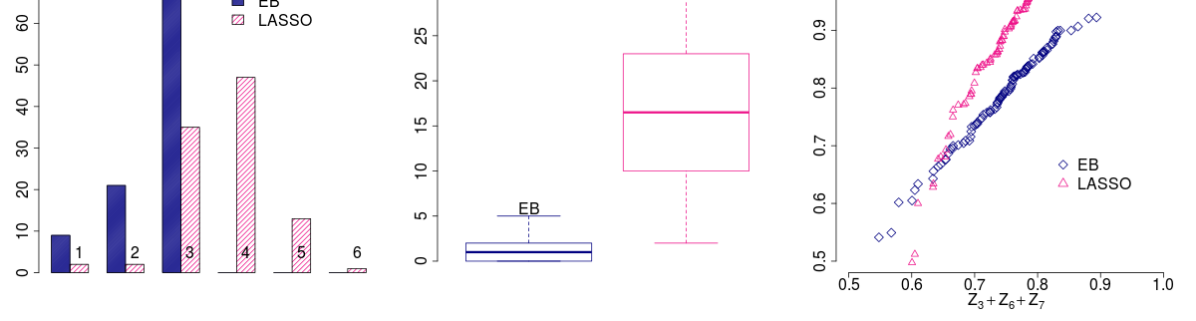
Figure 1: Simulation study – empirical Bayes method vs. the LASSO. Left (A): the number of ‘true positives’ selected by each method (from the set $Z_{1}-Z_{7}$). Recall that only one of $Z_{1}-Z_{4}$ and only one of $Z_{5}-Z_{6}$ should be included in the model, in order to avoid multicollinearity. Middle (B): The number of false positives obtained from each method. Right (C): The $R^{2}$ values obtained by each method vs. the true $R^{2}$ when fitting the correct model, $Y=Z_{3}+Z_{6}+Z_{7}$.

Figure 1 summarizes the differences between our empirical Bayes (EB) approach and the LASSO. Panel A (left) shows the number of variables among $Z_{1}-Z_{7}$ that were selected in each run. Recall that the high correlation between variables implies that there should be three variables from this subset in the model, and any additional variable will introduce a multicollinearity problem. The EB approach never had more than three variables from the set $Z_{1}-Z_{7}$ ($Z_{7}$, as well as one from $Z_{1}-Z_{4}$, and one from $Z_{5}-Z_{6}$), and 70% of the time it had the correct number of variables. The LASSO, on the other hand, selected up to 6 of the 7 variables, and over 60% of the times the selected model had too many variables from the set $Z_{1}-Z_{7}$.

Panel B (middle) shows the number of variables from the set $Z_{9}-Z_{301}$ that were selected in each model. The LASSO had a large number of ‘false positives’ with a median of 18.5, whereas our EB approach had a small number, with a median of 1. Note that in most cases the small number of false positives that were included in models by our method were indeed significant when we fitted the linear model. As mentioned earlier, in the simulation it can happen that some variables which were intended to be ‘null’ actually end up explaining a fairly large percent of the variability in the response, just by chance.

In the right panel (C) the $R^{2}$ values obtained from both methods are plotted versus the true $R^{2}$ values (on the x-axis) which are obtained when we fit the correct model, $Y_{i}=Z_{3i}+Z_{6i}+Z_{7i}+Z_{8i}+\epsilon_{i}$. The blue diamonds and the pink triangles represent the EB approach and the LASSO, respectively. The LASSO inflates the $R^{2}$ by including so many false positive variables in the model. In contrast, our method yields values which are approximately equal to the true values. Our $R^{2}$ values are typically slightly higher than the ‘true’ $R^{2}$ because when our method selected variables from the ‘null’ set, these additional variables were actually significant when we fit the linear model.

Using the same simulation configuration, but with $N=80$ our empirical Bayes approach always selects exactly three variables from the non-null set. In contrast, the LASSO selected three true positives 22% of the time, and 78% of the time it selected 4-7 non-null variables (yielding a model with multicollinearity).

The number of false positives resulting from our model decreases with the sample size, and when $N=80$, 78% of the runs having no false positives, 14% have one false positive, 6% have two false positives, and 2% have 3. The number of false positives resulting from the LASSO was very high and similar to the case of $N=40$ (as depicted in Figure 1, B) with a median of 19.

6 Case Studies

6.1 The Riboflavin Data

In a recent paper demonstrating modern approaches to high-dimensional statistics, Bühlmann et al. (2014) used a data set in which the response variable is the logarithm of riboflavin (vitamin B12) production rate, and there are normalized expression levels of 4,088 genes which are used as explanatory variables. The sample size in this data set is $N=71$. In addition to the fact that the number of putative variable greatly exceeds the number of observations, many of the putative variables are highly correlated. Out of 8,353,828 pairs of genes, there are 70,349 with correlation coefficient greater than 0.8 (in absolute value).

Bühlmann et al. (2014) report that the Lasso with subsamples of size $B=500$, and with $q=20$ variables that enter the regularization step first, yields three significant and stable genes: LYSC_at, YOAB_at, and YXLD_at. The model with these three variables has an adjusted $R^{2}$ of 0.66, and AIC of 118.6. Their multisample-split method yields one significant variable (YXLD_at), and the projection estimator, used with Ridge-type score yields no significant variables at the FWER-adjusted 5% significance level. The model with just YXLD_at has an adjusted $R^{2}$ of 0.36 and AIC of 162.

Lederer and Müller (2015) also used this data set, to demonstrate their TREX model. Their final model includes three genes: YXLE_at, YOAB_at, and YXLD_at. The adjusted $R^{2}$ of their model is 0.6, and the AIC is 130.68. Two of the genes are highly correlated (YXLD_at and YXLE_at) and yield a variance inflation factor of 23.7 each, so when fitting the final linear regression model neither appears to be significant.

We ran our algorithm using both the greedy and the weighted probability methods as described in Section 3.3. The greedy method yielded five significant genes, with AIC=58.83 and an adjusted $R^{2}$ of 0.86. We ran the algorithm using the weighted probability method 100 times. The best model included seven genes, and had an AIC of 39.2 and an adjusted $R^{2}$ of 0.895. The median AIC among the 100 fitted models was 84.38, and the maximum AIC was 114.1. In summary, both methods yielded better fitting models than the ones obtained by Bühlmann et al. (2014) and Lederer and Müller (2015). Table 1 provides goodness-of-fit statistics for the different methods, including the Aikake Information Criterion (AIC), the coefficient of multiple determination ($R^{2}$), and the mean absolute error (MAE). Note that our best model explains 90.5% of the variability in the data. Figure (2) shows the observed values (Y) vs. the fitted values from three models: Lederer and Müller (2015), Bühlmann et al. (2014), and our ‘weighted probability’ (best fit). In addition to having much smaller residuals than the two other methods, our method provides much better prediction for low values of riboflavin. The other two methods seem to over-estimate the riboflavin levels when the true (normalized) values are small (less than $-9$).

Method	AIC	$R^{2}$	MAE
Lederer and Müller (2015)	130.681	0.616	0.462
Bühlmann et al. (2014)	118.625	0.676	0.411
‘greedy’	58.828	0.879	0.244
‘weighted probability’ (best fit)	39.223	0.905	0.219

Table 1: Goodness of fit statistics for the different methods - the riboflavin data.

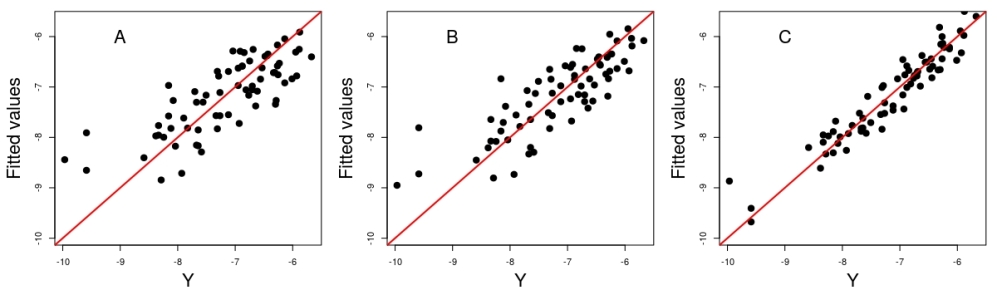
Figure 2: Riboflavin data – fitted vs. observed values. A: Lederer and Müller (2015), B: Bühlmann et al. (2014), C: our ‘weighted probability’ (best fit).

Table 2 provides the parameter estimates for the best model which was obtained using our weighted probability method. All seven variables are significant and they all have low variance inflation factors, indicating that the selected variables are not highly correlated.

	Estimate	Std. Error	t value	Pr($>|t|$)	VIF
(Intercept)	-7.60	0.06	-135.32	0.00	1.00
ARGF_at	-0.86	0.09	-9.28	0.00	1.24
XHLB_at	0.69	0.16	4.31	0.00	2.90
XKDN_at	-0.51	0.15	-3.43	0.00	3.14
XKDS_at	0.43	0.19	2.21	0.03	3.77
YHDZ_at	0.46	0.09	5.21	0.00	1.41
YOAB_at	-1.13	0.10	-11.29	0.00	1.35
YXLE_at	-0.92	0.09	-10.39	0.00	1.41

Table 2: Parameter estimates for the best fitting model - the riboflavin data.

Clearly, our method found an excellent combination of a small number of putative variables that explain over 90% of the variability in the data, and none of these putative variables is approximately a linear combination of the others. However, one should be careful not to interpret it as the ‘right model’ for two reasons. First, when the number of putative variables is large there is no way to evaluate all possible models. Second, if two genes are highly correlated and one of them is found to be significantly associated with the outcome, then we expect the other gene to also be associated with the outcome. Thus, we recommend to run the randomized version of our algorithm and analyze the relationships between selected variables, as we demonstrate now.

Among the 191 variables that were selected by our method in at least one iteration of the weighted probability method there are 64 highly correlated pairs (absolute value of the correlation coefficient greater than 0.8). Now consider the seven variables in the best fitting model. Table 3 shows the number of models in which each of these variables was included. Three of the variables actually represent a set of highly correlated genes. For example, ARGF_at was selected 8 times, but it is highly correlated with three other genes (ARGD_at, ARGH_at, and ARGJ_at) which were selected a total of 4 times. So this set of related genes was selected in 12 of the models. The cluster of genes which are correlated with XHLB_at consists of 7 genes and was represented in 95 of the models. Similarly, YXLE_at represents a cluster of 6 genes, of which one was included in 97 of the models. The large number of models which included a variable from the XHLB_at and YXLE_at clusters suggests that the final model should include a representative from these clusters. Note that our model never selected more than one gene from the same cluster. The other four selected genes were not correlated with any other selected genes. Two of these genes (XKDS_at and YOAB_at) appear in a relatively large number of models (23 and 24, respectively).

Variable	# models	Correlated variables	# models	Total models
ARGF_at	8	ARGH_at, ARGJ_at, ARGD_at	2, 1, 1	12
XHLB_at	22	XKDF_at, XKDH_at, XKDI_at,	13, 2, 19,	95
		XKDK_at, XHLA_at, XLYA_at	9, 17, 13
XKDN_at	1			1
XKDS_at	23			23
YHDZ_at	3			3
YOAB_at	24			24
YXLE_at	18	YXLC_at, YXLD_at, YXLF_at,	6, 18, 23,	97
		YXLG_at, YXLJ_at	14, 18

Table 3: The riboflavin data - the number of models in which each selected variable was included. ARGF_at, XHLB_at, YXLE_at are correlated with other selected genes. The last column shows the total number of models (out of 100) in which each cluster of genes was represented.

6.2 The BMI Data

Lin et al. (2014) demonstrated an application of a LASSO-based variable selection method for regression models with compositional covariates. The analysis aims to identify a subset of 87 bacteria genera in the gut whose subcomposition is associated with body-mass index (BMI). The data in this case is compositional, which using our previous notation means that $\sum_{j=1}^{87}z_{ij}=1$ for each $i$. To apply our method directly, without changing the model to account for the sum constraint, we perform the log ratio transformation and replace the matrix $\mathbf{Z}$ with $\mathbf{Z}^{K}=[\log(z_{ij}/z_{iK})]$. The data contains many zero counts, so Lin et al. (2014) replace them with 0.5 before converting the data to be in compositional form. We analyzed the data with all 87 bacteria and obtained a model that includes all four variables in Lin et al. (2014) and two additional genera (Dorea and Oscillibacter). Wu et al. (2011) report that the Oscillibacter genus was negatively correlated with BMI, which agrees with our overall model. However, when we refit the six genera model we find that Oscillibacter is no longer significant ($p=0.657$).

In this section we summarize the results of our analysis using a subset of 45 bacteria which had non-zero counts in at least 10% of the samples ($N=96$). The omitted genera have minimal contribution to the overall distribution of the proportions. The Lin et al. (2014) analysis finds four genera (Acidaminococcus, Alistipes, Allisonella, Clostridium). The best model obtained by our algorithm includes 8 genera and it yields an increase of 7.5% in the amount of variability explained by the model when compared to the model obtained by Lin et al. (2014). However, when fitting the regression model with the selected genera we observe that two of them (Dorea and Oscillibacter) are not significant. We fit a reduced model with 6 genera (Acidaminococcus, Alistipes, Allisonella, Catenibacterium, Clostridium, Megamonas) and obtain the lowest AIC (564.5) and the largest adjusted $R^{2}$ (0.345). Some goodness of fit statistics for the different models can be found in Table 4, and the parameter estimates for the final model are provided in Table 5.

Method	Variables	AIC	$R^{2}$	MAE
Lin et al. (2014)	4	569.7	0.324	3.290
‘weighted probability’	8	566.5	0.399	3.123
‘weighted probability’ (reduced model)	6	564.5	0.386	3.158

Table 4: Goodness of fit statistics - the BMI data.

	Estimate	Std. Error	t value	Pr($>|t|$)
(Intercept)	28.41	1.49	19.01	0.00
Alistipes	-0.67	0.25	-2.73	0.01
Clostridium	-1.04	0.31	-3.33	0.00
Acidaminococcus	0.92	0.25	3.59	0.00
Allisonella	1.39	0.56	2.49	0.01
Megamonas	-0.86	0.33	-2.61	0.01
Catenibacterium	0.74	0.36	2.06	0.04

Table 5: Parameter estimates in the BMI data.

Our results are consistent with the previous findings in the microbiome literature. The relative proportion of phylum Bacteroidetes (containing the Alistipes genus) to phylum Firmicutes (all others genera found) is lower in obese mice and humans than in lean subjects (Ley et al., 2006). Furthermore the family Veillonellaceae (containing the Acidaminococcus and Allisonella genera) are positively correlated to BMI (Wu et al., 2011). The two additional genera found beyond Lin et al. (2014), Catenibacterium and Megamonas, have been found to be associated with BMI. Chiu et al. (2014) identifies Megamonas as a genus that differentiates between low and high BMI in a Taiwanese population and Turnbaugh et al. (2009) found that the Catenibacterium genus increased diet-induced dysbiosis for high-fat and high-sugar diets in humanized gnotobiotic mice.

7 Extensions

We briefly discuss a number of useful extensions to our model.

Mixed Models: In model (2) we assumed that the mean of the response is a linear combination of two groups of variables, where $\mathbf{X}\bm{\beta}$ represents the ‘locked’ variables, and $\mathbf{Z}\bm{\Gamma}\mathbf{u}$ represents the putative variables. We assumed that the ‘locked’ variables are treated as fixed effects in the model. There are situations in which we may want to ‘lock’ additional random effects in the model. For example, in biological applications (e.g. QTL analysis) one may want to include breed, or kinship information as a random effect. This can be done using the same method that we used to estimate the variance parameter, since the update equations for the EM algorithm extend to any number of variance components (see the general formulation of the estimation in Section 8.3.b in Searle et al. 1992). For example, with one additional random effect only one parameter is added to the model, which can be modified as follows:

$$\mathbf{y} = \mathbf{X}\bm{\beta}+\mathbf{Z}_{0}\mathbf{v}+\mathbf{Z}\bm{\Gamma}\mathbf{u}+\bm{\varepsilon}$$

$$\bm{\varepsilon} \sim N\left(\mathbf{0}_{N},\sigma_{e}^{2}\mathbf{I}_{N}\right)$$

$$\mathbf{Z}_{0}\mathbf{v} \sim N\left(\mathbf{0}_{N},\sigma_{0}^{2}\mathbf{I}\right)$$

$$\mathbf{Z}\bm{\Gamma}\mathbf{u} \sim N\left(\mathbf{Z}\bm{\Gamma}\bm{\mu},\sigma^{2}\mathbf{Z}\bm{\Gamma}^{2}\mathbf{Z}^{\prime}\right)\,.$$

Interactions: In many applications it may be useful to include interactions between fixed effects and all putative variables. For example, if the response is the Forced Expiratory Volume (FEV, which measures how much air is exhaled during a forced breath), it may be the case that the effects of interest are the interactions between gene expression levels (the putative variables) and smoking status (the fixed effects). It is possible that the genetic variables have a different effect on the response for heavy smokers than for non-smokers.

Generalized Linear Models: Our model can be extended to the generalized linear model framework. This will allow us to deal with binomial and Poisson responses, as well as censored survival times using the artificial Poisson model as described by Whitehead (1980). Suppose the response mean vector, $\bm{\mu}$, is related to the linear predictor, $\bm{\eta}=\mathbf{X}\bm{\beta}+\mathbf{Z}\mathbf{u}$, via a link function, $g(\bm{\mu})=\bm{\eta}$, and conditional on the latent indicator vector, $\bm{\gamma}$, the responses are independent outcomes from an exponential dispersion family; i.e.

$$f(y_{i}|\mathbf{u},\bm{\gamma})=h(y_{i})\exp\left\{\frac{w_{i}}{\phi}\left[\theta_{i}y_{i}-b(\theta_{i})\right]+c(y_{i};\phi/w_{i})\right\}$$ (13)

where the identity $\mu_{i}=b^{\prime}(\theta_{i})$ relates the canonical parameter for the $i$th response to its mean, $\phi$ is a (possibly known) dispersion parameter, and $w_{i}$ are known weights. In this setting implementation of the EM algorithm is further complicated by the fact that the complete data likelihood for $(\mathbf{y},\bm{\gamma})$ is not analytically tractable, with the exception being the normal response case, where it is given in (5).

An approximation of the intractable likelihood can be developed by using penalized quasi-likelihood (PQL) approaches proposed by Schall (1991), Breslow and Clayton (1993) and Wolfinger and O’Connell (1993). The basic idea of the PQL approach is to replace the generalized linear mixed model by an approximating linear mixed model, $\mathbf{z}=\mathbf{X}\bm{\beta}+\mathbf{Zu}+\mathbf{e}$, in which $\mathbf{e}=(\mathbf{y}-\bm{\mu})(\partial\bm{\eta}/\partial\bm{\mu})\sim N(0,\mathbf{W}^{-1})$, $\mathbf{u}\sim N(\psi\mathbf{1}_{M},\sigma^{2}_{u}\mathbf{I}_{K})$, and $\mathbf{W}=diag[w_{i}(\partial\mu_{i}/\partial\eta_{i})^{2}/\phi V(\mu_{i})]$, where $V(\cdot)$ denotes the variance function for the GLM. For fixed $\bm{\gamma}$, estimation of the model parameters proceeds in a similar manner to that for a normal theory linear mixed model, except that the working response vector, $\mathbf{z}$, must be iteratively updated. There are also a several different algorithms for estimating the variance components $(\phi,\sigma^{2}_{u})$ (see Pawitan, 2001). The key identity (10) is replaced by

$$\left(\mathbf{W}^{-1}+\sigma^{2}_{u}\mathbf{ZZ}^{\prime}\right)^{-1}=\mathbf{W}+\mathbf{Z}\left(\frac{1}{\sigma^{2}_{u}}\mathbf{W}+\mathbf{Z}^{\prime}\mathbf{W}\mathbf{Z}\right)^{-1}\mathbf{Z}^{\prime}\,,$$

with the $(k,l)$th component of $\mathbf{Z}^{\prime}\mathbf{W}\mathbf{Z}$ being $(\mathbf{z^{\prime}}_{k}\mathbf{W}\mathbf{z}_{l})\gamma_{k}\gamma_{l}$, so that threshold based on the posterior expected $\gamma$’s again results in a much lower dimensional matrix inversion at the M-step.

Developing methods to implement these extensions will be considered in future work.

8 Conclusion

In 1996 Brad Efron stated that variable selection in regression is the most important problem in statistics (Hesterberg et al., 2008). Since then many papers have been written on the topic, as this continues to be a challenging problem in the age of high-throughput sequencing in genomics, and as other types of ‘omics’ data become available and more affordable.

We developed a model-based, empirical Bayes approach to variable selection. We propose a mixture model in which the putative variables are modeled as random effects. This leads to shrinkage estimation and increases the power to select the correct variables, while maintaining a low rate of false positive selections. The mixture model involves a very small number of parameters. Importantly, that number remains constant regardless of the number of putative variables. This parsimony contributes to the scalability of the algorithm and it can handle a large number of predictors. In contrast, methods based on MCMC sampling often require the user to focus on a relatively small subset of the predictors. Using the EM algorithm and an efficient dimension reduction method our algorithm converges significantly faster than simulation-based methods. Furthermore, a simple modification to the algorithm prevents multicollinearity problems in the fitted regression model.

References

- Aitchison (1982) Aitchison, J. (1982). The statistical analysis of compositional data. Journal of the Royal Statistical Society. Series B (Methodological), 44 139–177.
- Akaike (1974) Akaike, H. (1974). A new look at the statistical model identification. IEEE Transactions on Automatic Control, 19 716–723.
- Bar et al. (2010) Bar, H., Booth, J., Schifano, E. D. and Wells, M. T. (2010). Laplace approximated em microarray analysis: An empirical Bayes approach for comparative microarray experiments. Statistical Science, 25 388–407.
- Benjamini and Gavrilov (2009) Benjamini, Y. and Gavrilov, Y. (2009). A simple forward selection procedure based on false discovery rate control. Ann. Appl. Stat., 3 179–198.
- Benjamini and Hochberg (1995) Benjamini, Y. and Hochberg, Y. (1995). Controlling the false discovery rate-a practical and powerful approach to multiple testing. Journal of The Royal Statistical Society Series B, 57 499–517.
- Bogdan et al. (2014) Bogdan, M., van den Berg, E., Sabatti, C., Su, W. and Candes, E. (2014). Slope – adaptive variable selection via convex optimization. arXiv:1407.3824. URL http://arxiv.org/abs/1407.3824.
- Boisbunon et al. (2014) Boisbunon, A., Canu, S., Fourdrinier, D., Strawderman, W. and Wells, M. T. (2014). Akaike’s information criterion, and estimators of loss for elliptically symmetric distributions. International Statistical Review, 82 422–439.
- Bondell and Reich (2012) Bondell, H. D. and Reich, B. J. (2012). Consistent high-dimensional Bayesian variable selection via penalized credible regions. Journal of the American Statistical Association, 107 1610–1624.
- Breiman (1995) Breiman, L. (1995). Better subset regression using nonnegative garrote. Technometrics, 104 373–384.
- Breslow and Clayton (1993) Breslow, N. E. and Clayton, D. (1993). Approximate inference in generalized linear mixed models. Journal of the American Statistical Association, 88 9–25.
- Bühlmann et al. (2014) Bühlmann, P., Kalisch, M. and Meier, L. (2014). High-dimensional statistics with a view toward applications in biology. Annual Review of Statistics and Its Application, 1 255–278.
- Candes and Tao (2005) Candes, E. J. and Tao, T. (2005). Decoding by linear programming. Information Theory, IEEE Transactions, 51 4203–4215.
- Casella and Moreno (2006) Casella, G. and Moreno, E. (2006). Objective Bayesian variable selection. Journal of the American Statistical Association, 101 157–167.
- Chiu et al. (2014) Chiu, C.-M., Huang, W.-C., Weng, S.-L., Tseng, H.-C., Liang, C., Wang, W.-C., Yang, T., Yang, T.-L., Weng, C.-T., Chang, T.-H. et al. (2014). Systematic analysis of the association between gut flora and obesity through high-throughput sequencing and bioinformatics approaches. BioMed Research International, 2014.
- Dempster et al. (1977) Dempster, A. P., Laird, N. M. and Rubin, D. B. (1977). Maximum likelihood from incomplete data via the EM algorithm. Journal Of The Royal Statistical Society, Series B, 39 1–38.
- Efron et al. (2004) Efron, B., Hastie, T., Johnstone, I. and Tibshirani, R. (2004). Least angle regression. Annals of Statistics, 32 407–499.
- Fan and Li (2001) Fan, J. and Li, R. (2001). Variable selection via nonconcave penalized likelihood and its oracle properties. Journal of the American Statistical Association, 96 1348–1360.
- George and McCulloch (1993) George, E. and McCulloch, R. (1993). Variable selection via Gibbs sampling. Journal of the American Statistical Association, 88 881–889.
- Golub and Van Loan (1996) Golub, G. and Van Loan, C. (1996). Matrix Computations. The Johns Hopkins University Press, Baltimore, MD, US.
- Guan and Stephens (2012) Guan, Y. and Stephens, M. (2012). Bayesian variable selection regression for genome-wide association studies and other large-scale problems. Annals of Applied Statistics, 5 1780–1815.
- Hastie and Efron (2013) Hastie, T. and Efron, B. (2013). lars: Least Angle Regression, Lasso and Forward Stagewise. R package version 1.2, URL http://CRAN.R-project.org/package=lars.
- Hebiri and Lederer (2013) Hebiri, M. and Lederer, J. (2013). How correlations influence lasso prediction. Information Theory, IEEE Transactions on, 59 1846–1854.
- Hesterberg et al. (2008) Hesterberg, T. C., Choi, N. H., Meier, L. and Fraley, C. (2008). Least angle and L1 penalized regression: A review. Statistics Surveys, 2 61–93.
- Hocking (1976) Hocking, R. R. (1976). The analysis and selection of variables in linear regression. Biometrics, 32 661–675.
- Ishwaran and Rao (2005) Ishwaran, H. and Rao, J. S. (2005). Spike and slab variable selection: Frequentist and Bayesian strategies. Annals of Statistics, 33 730–773.