Optimal Time-Reversed Wideband Signals for Distributed Sensing

Abstract

This paper considers a distributed wave-based sensing system that probes a scene consisting of multiple interacting idealized targets. Each sensor is a collocated transmit-receive pair that is capable of transmitting arbitrary wideband waveforms. We address the problem of finding the space-time transmit waveform that provides the best target detection performance in the sense of maximizing the energy scattered back into the receivers. Our approach is based on earlier work that constructed the solution by an iterative time-reversal (TR) process. In particular, for the case of idealized point-like scatterers in free space, we examine the frequency dependence of the eigenvalues of the TR operator, and we show that their behavior depends on constructive and destructive interference of the waves traveling along different paths. In addition, we show how these eigenvalues are connected to the poles of the Singularity Expansion Method. Our study of the frequency behavior distinguishes this work from most previous TR work, which focused on single-frequency waveforms and noninteracting targets. The main result of the present paper is that the TR process provides an automated, guaranteed way to find the resonant frequencies of the scattering system.

I Introduction

This paper addresses the problem of finding the space-time waveform that results in the most energy scattered back to the sensors from a distant target. We consider the case in which a small number of ideal discrete sensors both transmit and receive, so that the problem becomes one of determining the time-domain waveforms that should be transmitted by the different sensors so that those sensors receive the maximum scattered energy.

The problem of increasing the scattered energy received by the sensors has been previously studied by a number of authors. For a single sensor, [1] proposed an approach based on trying dfferent frequencies in a random sequence. For multiple sensors, received signal energy can be increased by a process known as Time Reversal (TR) or Décomposition de l’Opérateur de Retournement Temporel (DORT), in which scattered signals are recorded at the receivers and then time-reversed and retransmitted. The TR idea, which has its roots in optical phase conjugation, has been used in numerous studies in acoustics and electromagnetism [2, 3, 4, 5], and has potential applications ranging from sensing (remote imaging, radar, acoustics, optics, etc.) to communications [4, 6, 7, 3].

The lynchpin of the single-frequency TR approach is the application of the classical mathematical theorem known as the Power Method, which guarantees that under mild conditions, the application of successive powers of an operator to an arbitrary seed vector results in a sequence of vectors that converges to the eigenvector associated with the maximum eigenvalue [8]. In the sensing context, the relevant operator is the TR operator, which is the product of the scattering operator and its adjoint. The “largest eigenvector” (i.e., the eigenvector corresponding to the largest eigenvalue) corresponds to specifying the relative strengths and phases of the transmitted fields in a way that causes the most energy to scatter back to the receivers. This eigenvector contains information about the scatterers: [9, 10] showed that for point-like scatterers, the temporal wavefield focuses on the strongest scatterer [11, 12]; for a single spherical target, [13] showed that this eigenvector contains information about the target size and composition. The work [14, 15] showed that use of TR can improve target detection. These analyses were all carried out for waveforms of a single temporal frequency under the single-scattering assumption (Born approximation).

Analysis of the TR temporal behavior for the general case of multiple scattering was investigated by [16, 17], through an analysis of the frequency dependence of the TR operator. This work showed that in general the time-domain TR construction converges automatically to a certain single-frequency waveform. The frequency of this limiting waveform is a resonance, namely a frequency at which the largest eigenvalue has a local maximum, and the waveform’s spatial shape (which determines its radiation pattern) is given by the corresponding eigenvector. Thus the time-domain TR process can be used to tune automatically to the space-time waveform that is optimal in the sense of providing the best target detection performance. These predictions of Cheney et al. [16, 17] are consistent with experimental observations reported by [18, 3, 9, 11], who noticed that as the iterative TR process proceeds, the pulse temporally broadens, the frequency can shift, and the spectrum narrows. The predictions are also consistent with the simulations of [19], who also found that the iterative TR process converges to a time-harmonic waveform.

This paper carries out a detailed analysis of the case of two sensors and two point-like scatterers, where the scatterers are “interacting” in the sense that there is multiple scattering between them. In particular, we obtain formulas for the scattering operator and the associated resonances; we show that these resonances arise from constructive interference between the various scattered waves. We show, moreover, that the TR method provides a stable experimental method for finding these resonances.

Our explicit consideration of multiple scattering is one aspect that differentiates this work from previous TR analysis.

Another important connection between the present paper and earlier work is its relation to the Singularity Expansion Method (SEM) [20]. Specifically, the poles of the SEM are associated with information derived from the iterative TR process. The analysis of the eigenvalues associated with the TR matrix leads to an understanding of the relationship between the poles of the SEM and the eigenvalues of the TR matrix. In particular, the poles of the SEM appear in the expression for the scattered field. Here our approach uses Fourier analysis to avoid issues with the two-sided Laplace transform in existing SEM analyses.

This paper is organized as follows. In Section II, we provide some mathematical background on scattering theory. In Section III, we specialize to the case of two point scatterers and two transmit/receive pairs, where the Foldy-Lax method [21, 22] is used to obtain the scattering operator. In Section III-C, we obtain explicit analytical expressions for the scattering operator and its spectral decomposition. In Section IV, we outline the TR process and discuss its behavior in the two-target, two-sensor case. In Section V, we discuss the connection to the SEM poles. In Section VI, we show that the TR process and the eigenvalue information obtained from it are stable with respect to noise. In Section VII, we show simulation results. Section VIII gives conclusions and suggestions for future work.

II Mathematical Formulation and Derivation

We begin by solving the simplified scalar model of the wave equation for the time-domain electric field $E$,

$$\left(\nabla^{2}-\frac{1}{c^{2}(\mathbf{r})}\frac{\partial^{2}}{\partial t^{2}}\right)E(\mathbf{r},t)=0,$$ (1)

where we think of $c(\mathbf{r})$ as the local speed of propagation of the electromagnetic (EM) waves in a specified media. In free space, the speed is $c_{0}$. Scattering can be thought of as being produced by changes in the wave speed with perturbation (scattering potential)

$$V(\mathbf{r})=\frac{1}{c_{0}^{2}}-\frac{1}{c^{2}(\mathbf{r})}.$$ (2)

Under the Fourier Transform pair

$$\tilde{E}(\mathbf{r},\omega)=\int_{-\infty}^{\infty}E(\mathbf{r},t)e^{-j\omega t}\>\mathrm{d}t,$$ (3)

$$E(\mathbf{r},t)=\frac{1}{2\pi}\int_{-\infty}^{\infty}\tilde{E}(\mathbf{r},\omega)e^{j\omega t}\>\mathrm{d}\omega,$$ (4)

(3) converts (1) into

$$(\nabla^{2}+k^{2}-\omega^{2}V(\mathbf{r}))\tilde{E}=0,$$ (5)

where $k=\omega/c_{0}$. The convention throughout is that a tilde denotes a frequency-domain quantity.

The relevant free-space fundamental solution $\tilde{G}$, which satisfies

$$(\nabla^{2}+k^{2})\tilde{G}=-\delta(\mathbf{r}),$$ (6)

is the Green’s function

$$\tilde{G}(\mathbf{r},\omega)=-\frac{e^{-jk\|\mathbf{r}\|}}{4\pi\|\mathbf{r}\|},$$ (7)

where $\|\cdot\|$ is the Euclidean norm, and $\delta$ is the Dirac delta.

For a radiation source

$$\tilde{F}(\mathbf{r},\omega)=\mu_{0}j\omega\tilde{J}(\mathbf{r},\omega),$$ (8)

where $\mu_{0}$ is the permeability of free space and $\tilde{J}$ is a scalar current density, the solution to the inhomogeneous wave equation

$$\left(\nabla^{2}+k^{2}\right)\tilde{E}_{\mathrm{in}}(\mathbf{r},\omega)=\tilde{F}(\mathbf{r},\omega)$$ (9)

is the radiated field

$$\tilde{E}_{\mathrm{in}}(\mathbf{r},\omega)=\int\limits_{\Omega}\tilde{G}(\mathbf{r}-\mathbf{y},\omega)\tilde{F}(\mathbf{y},\omega)\>\mathrm{d}\mathbf{y},$$ (10)

where the volume $\Omega$ of the source is a subset of $\mathbb{R}^{3}$ and $d\mathbf{y}$ denotes the volume element.

The total field $\tilde{E}_{\mathrm{tot}}$ due to the source in the presence of scatterers satisfies

$$\left(\nabla^{2}+k^{2}-\omega^{2}V(\mathbf{r})\right)\tilde{E}_{\mathrm{tot}}(\mathbf{r},\omega)=\tilde{F}(\mathbf{r},\omega).$$ (11)

We can write the total field as a sum of the incident field in (10) plus the scattered field generated by a target, $\tilde{E}_{\mathrm{tot}}=\tilde{E}_{\mathrm{in}}+\tilde{E}_{\mathrm{sc}}$ [23]. Subtracting (9) from (11) yields

$$\left(\nabla^{2}+k^{2}\right)\tilde{E}_{\mathrm{sc}}(\mathbf{r},\omega)=-V(\mathbf{r})\omega^{2}\tilde{E}_{\mathrm{tot}}(\mathbf{r},\omega).$$ (12)

By convolving both sides of (12) with $\tilde{G}$, we obtain the Lippmann-Schwinger equation for the scattered field at an arbitrary observation point $\mathbf{r}$

$$\tilde{E}_{\mathrm{sc}}(\mathbf{r},\omega)=\int\limits_{\Omega}\tilde{G}(\mathbf{r}-\mathbf{y},\omega)\omega^{2}V(\mathbf{y})\tilde{E}_{\mathrm{tot}}(\mathbf{y},\omega)\>\mathrm{d}\mathbf{y}.$$ (13)

Equation (13) is a Fredholm integral equation of the second kind [24, pp. 98-101] and can be solved by a variety of different methods. This Lippmann-Schwinger equation provides a framework for constructing the map from the source $\tilde{F}$ to the fields at observation point $\mathbf{r}$. We call this map the scattering operator $S$.

In the next section, we work out the explicit special case of a scattering operator for 2 point scatterers and 2 transmit/receive pairs.

III Scattering Operator for two point scatterers and two transmit/receive pairs

In this section, we examine the scattering operator $S$ for the special case of two point scatterers and two transmit/receive pairs of sensors. First the incident, scattered, and total fields are derived using the Foldy-Lax method [25, 21, 22]. Then $S$ is obtained and recast in terms of three physically interpretable matrices: the forward and back-scattered propagators associated with the paths between sensors and scatterers; and an interaction matrix that characterizes the interactions among the scatterers.

The wave speed perturbation $V$ in (2) can be modeled as a sum of point scatterers. For two point scatterers, located at $\mathbf{x}_{1}$ and $\mathbf{x}_{2}$, (2) becomes

$$V(\mathbf{r})=\sum_{m=1}^{2}q_{m}\delta(\mathbf{r}-\mathbf{x}_{m}),$$ (14)

where $q_{m}$ is the scattering strength or the reflectivity of the $m$th target.

III-A Foldy-Lax Method

We use the Foldy-Lax method [25, 21, 22] to obtain an explicit expression for the scattering operator. The Foldy-Lax method requires solving the set of linear equations ($n=1,2$):

$$\tilde{E}^{n}(\mathbf{x}_{n},\omega) =\tilde{E}_{\mathrm{in}}(\mathbf{x}_{n},\omega)$$

$$+\sum_{m\neq n}\tilde{G}(\mathbf{x}_{n}-\mathbf{x}_{m},\omega)\omega^{2}q_{m}\tilde{E}^{m}(\mathbf{x}_{m},\omega).$$ (15)

Here $\tilde{E}^{m}$ denotes the “locally incident field” at the scatterer $m$, namely the incident field seen by the $m$th scatterer. Equation (III-A) expresses the incident field at the scattering location $\mathbf{x}_{n}$ as a sum of the overall incident field $\tilde{E}_{\mathrm{in}}$ plus the sum of the scattered fields from all of the other scatterers.

In (13) we use (14) and substitute the “locally incident field” of (III-A) for the “total” field $\tilde{E}_{\mathrm{tot}}$ at the appropriate scatterer. The scattered field is then

$$\tilde{E}_{\mathrm{sc}}(\mathbf{r},\omega)=\sum_{m=1}^{2}\tilde{G}(\mathbf{r}-\mathbf{x}_{m},\omega)\omega^{2}q_{m}\tilde{E}^{m}(\mathbf{x}_{m},\omega).$$ (16)

Figure 1 shows the possible direct paths of the fields to the point scatterers and their scattered returns.

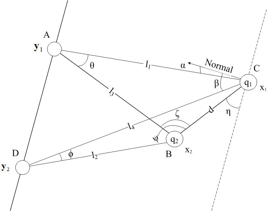
Figure 1: Scattering geometry. $\mathbf{y}_{i}$ denotes the transmit/receive pairs at points $C$ and $D$. $l_{i}$ denotes the distances from the $\mathbf{y}_{i}$ to the scatterer at $\mathbf{x}_{k}$ at Points $A$ and $B$ with reflectivity coefficient $\mu_{k}$.

We re-write (III-A) in matrix form

$$\left(\begin{array}[]{cc}1&-\omega^{2}q_{2}\tilde{G}(\mathbf{d},\omega)\\ -\omega^{2}q_{1}\tilde{G}(\mathbf{d},\omega)&1\end{array}\right)$$ (19)

$$\times \left(\begin{array}[]{c}\tilde{E}^{1}(\mathbf{x}_{1},\omega)\\ \tilde{E}^{2}(\mathbf{x}_{2},\omega)\end{array}\right)=\left(\begin{array}[]{c}\tilde{E}_{\mathrm{in}}(\mathbf{x}_{1},\omega)\\ \tilde{E}_{\mathrm{in}}(\mathbf{x}_{2},\omega)\end{array}\right),$$ (24)

where $\mathbf{d}=\mathbf{x}_{1}-\mathbf{x}_{2}$. The solution to (19) is

$$\tilde{E}^{1}(\mathbf{x}_{1},\omega)=\frac{\tilde{E}_{\mathrm{in}}(\mathbf{x}_{1},\omega)+q_{2}\omega^{2}\tilde{G}(\mathbf{d})\tilde{E}_{\mathrm{in}}(\mathbf{x}_{2},\omega)}{1-\omega^{4}q_{1}q_{2}\tilde{G}^{2}(\mathbf{d})}$$ (25)

$$\tilde{E}^{2}(\mathbf{x}_{2},\omega)=\frac{\tilde{E}_{\mathrm{in}}(\mathbf{x}_{2},\omega)+q_{1}\omega^{2}\tilde{G}(\mathbf{d})\tilde{E}_{\mathrm{in}}(\mathbf{x}_{1},\omega)}{1-\omega^{4}q_{1}q_{2}\tilde{G}^{2}(\mathbf{d})}$$ (26)

where for notational convenience we have suppressed the $\omega$ argument in $\tilde{G}$. Substituting (25) and (26) into (16) implies

$$\tilde{E}_{\mathrm{sc}}(\mathbf{r},\omega)= \omega^{2}q_{1}\tilde{G}(\mathbf{r}-\mathbf{x}_{1})$$

$$\times \frac{\tilde{E}_{\mathrm{in}}(\mathbf{x}_{1},\omega)+\omega^{2}q_{2}\tilde{G}(\mathbf{d})\tilde{E}_{\mathrm{in}}(\mathbf{x}_{2},\omega)}{1-\omega^{4}q_{1}q_{2}\tilde{G}^{2}(\mathbf{d})}$$

$$+\omega^{2}q_{2}\tilde{G}(\mathbf{r}-\mathbf{x}_{2})$$

$$\times \frac{\tilde{E}_{\mathrm{in}}(\mathbf{x}_{2},\omega)+\omega^{2}q_{1}\tilde{G}(\mathbf{d})\tilde{E}_{\mathrm{in}}(\mathbf{x}_{1},\omega)}{1-\omega^{4}q_{1}q_{2}\tilde{G}^{2}(\mathbf{d})}.$$ (27)

Note that when $\omega^{4}q_{1}q_{2}\tilde{G}^{2}(\mathbf{d})<1$, the denominator of (III-A) can be expanded in a geometric series, and in the resulting expression, each term can be interpreted in terms of scattering and propagation between sensors and scatterers. This interpretation is discussed in more detail in Section IV-B.

III-B Incident field and scattering matrix

In this example, the source in (8) is the sum of point-like sources from the transmitter locations $\mathbf{y}_{i}$

$$\tilde{F}(\mathbf{r},\omega)=\sum\limits_{i=1}^{2}\mu_{0}j\omega\tilde{J}_{i}(\omega)\delta(\mathbf{r}-\mathbf{y}_{i}).$$ (28)

Consequently, the incident field in (10) is

$$\tilde{E}_{\mathrm{in}}(\mathbf{r},\omega)= \sum\limits_{i=1}^{2}-\mu_{0}j\omega\tilde{J}_{i}(\omega)\frac{e^{-jk\|\mathbf{r}-\mathbf{y}_{i}\|}}{4\pi\|\mathbf{r}-\mathbf{y}_{i}\|}.$$ (29)

Next we substitute (29) into (III-A) and evaluate the scattered field $\tilde{E}_{\mathrm{sc}}(\mathbf{r},\omega)$ at the sensor location $\mathbf{r}=\mathbf{y}_{i}$ to obtain the received signal for the $i$th sensor. We denote this received field as

$$\tilde{R}_{i}(\omega)=\tilde{E}_{\mathrm{sc}}(\mathbf{y}_{i},\omega)$$

$$=\sum_{k=1}^{2}\frac{\mu_{0}j\omega\tilde{J}_{k}(\omega)}{\xi}\sum_{n=1}^{2}\tilde{G}(\mathbf{y}_{i}-\mathbf{x}_{n},\omega)q_{n}\omega^{2}\times$$

$$[\tilde{G}(\mathbf{x}_{n}-\mathbf{y}_{k},\omega)+q_{(n\;\mathrm{mod}\;2)+1}\omega^{2}\tilde{G}(\mathbf{d},\omega)$$

$$\times\tilde{G}(\mathbf{x}_{(n\;\mathrm{mod}\;2)+1}-\mathbf{y}_{k},\omega)],$$ (30)

where $(n\;\mathrm{mod}\;2)+1$ is equal to 1 when $n=2$ and 2 when $n=1$, and

$$\xi=1-q_{1}q_{2}\omega^{4}\tilde{G}^{2}(\mathbf{d},\omega).$$ (31)

The parameter $\xi$ is the determinant of the matrix in (19) and describes how the fields scatter between the two point scatterers. If the scattering between the two scatterers is weak, we can assume $\xi\approx 1$. It turns out that $\xi$ is an important parameter that contributes key information about the resonant frequencies of the scattering system, a fact that is discussed in more detail below.

In (III-B), define the inner summand as

$$S_{ik}= \frac{1}{\xi}\sum_{n=1}^{2}\tilde{G}(\mathbf{y}_{i}-\mathbf{x}_{n},\omega)\omega^{2}q_{n}$$

$$\times [\tilde{G}(\mathbf{x}_{n}-\mathbf{y}_{k},\omega)+\omega^{2}q_{(n\;\mathrm{mod}\;2)+1}\tilde{G}(\mathbf{d},\omega)$$

$$\times \tilde{G}(\mathbf{x}_{(n\;\mathrm{mod}\;2)+1}-\mathbf{y}_{k},\omega)].$$ (32)

The square matrix $(S_{ik})$ is the standard scattering operator $S$, also known as the multistatic data matrix or the transfer matrix. The matrix $S$ maps the transmitted signal vector

$$T(\omega)=\left[\begin{array}[]{c}\mu_{0}j\omega\tilde{J}_{1}(\omega)\\ \mu_{0}j\omega\tilde{J}_{2}(\omega)\end{array}\right],$$ (33)

to the received signal vector

$$R(\omega)=\left[\begin{array}[]{c}\tilde{R}_{1}(\omega)\\ \tilde{R}_{2}(\omega)\end{array}\right].$$ (34)

The components of these signal vectors are the transmitted and induced current densities at sensors 1 and 2, respectively.

III-C Analysis of the scattering matrix

On careful examination, (III-B) can be expressed as

$$S=\frac{\omega^{2}}{\xi}P\Delta P^{T},$$ (35)

the product of two propagator matrices ($P$ and $P^{T}$) and an interaction matrix $(\Delta)$, where

$$\Delta=\left[\begin{array}[]{cc}q_{1}&q_{1}q_{2}\omega^{2}\tilde{G}(\mathbf{d},\omega)\\ q_{1}q_{2}\omega^{2}\tilde{G}(\mathbf{d},\omega)&q_{2}\end{array}\right],$$ (36)

$$P=\left[\begin{array}[]{cc}\tilde{G}(\mathbf{y}_{1}-\mathbf{x}_{1},\omega)&\tilde{G}(\mathbf{y}_{1}-\mathbf{x}_{2},\omega)\\ \tilde{G}(\mathbf{y}_{2}-\mathbf{x}_{1},\omega)&\tilde{G}(\mathbf{y}_{2}-\mathbf{x}_{2},\omega)\end{array}\right],$$ (37)

and the superscript $T$ denotes matrix transposition. All three matrices are physically interpretable. In particular, P is an operator that maps the fields at the scatterer locations $\mathbf{x}_{1}$ and $\mathbf{x}_{2}$ to the corresponding fields at receiver locations $\mathbf{y}_{1}$ and $\mathbf{y}_{2}$. The transpose $P^{T}$ maps the fields from the transmitters located at $\mathbf{y}_{1}$ and $\mathbf{y}_{2}$ to the fields at the scatterers. The interaction matrix $\Delta$ describes the field interactions due to the scatterers.

The interaction matrix is singular at the frequencies $\omega_{\alpha}$ for which

$$\xi(\omega_{\alpha})=1-q_{1}q_{2}\omega_{\alpha}^{4}\tilde{G}^{2}(\mathbf{d},\omega_{\alpha})=0.$$ (38)

We note also that the interaction matrix $\Delta$ is aspect-independent; in other words, it does not depend on the spatial relationship between the targets and sensors. Consequently, it could be useful for various applications such as target classification. Unfortunately, the interaction matrix (36) cannot be measured directly; instead the scattering matrix (35) is the measurable quantity. The scattering matrix $S$ depends on the viewing angles between sensors and targets because the propagator matrices (37) do.

One case in which the scattering matrix can be used to obtain information about the scatterers is when the coupling between the scatterers, namely $q_{1}q_{2}\omega^{4}\tilde{G}^{2}(\mathbf{d},\omega)$, is weak. In this case, the off-diagonal elements of $\Delta$ are negligible, and $\xi=1$ from (31). This case was addressed in [26, 10], which showed that with enough sensors, the $n$th eigenvalue of the scattering matrix corresponds to the $n$th strongest scatterer.

In this paper we consider the more general case in which there is coupling between the two scatterers; that is, we take into account the effects of multiple scattering between the two scatterers. In this case, the eigenvalues of the scattering operator do not necessarily correspond to individual scatterers. To understand the connection between eigenvalues and the scattering strengths $q_{i}$, we carry out the following analysis. For notational convenience, we omit explicit references to frequency in the Green’s function, eigenvalues, and the operators unless it is required.

III-D Spectral decomposition of interaction matrix $\Delta$

The eigenvalues of $\Delta$ are

$$\lambda_{1,2}=\frac{(q_{1}+q_{2})\pm\sqrt{(q_{1}-q_{2})^{2}+4(q_{1}q_{2}\tilde{G}(\mathbf{d})\omega^{2})^{2}}}{2}$$ (39)

and the corresponding eigenvectors are

$$X_{1} =\left[\begin{array}[]{cc}-\frac{-q_{1}+q_{2}-\sqrt{(q_{1}-q_{2})^{2}+4(q_{1}q_{2}\tilde{G}(\mathbf{d})\omega^{2})^{2}}}{2\omega^{2}\tilde{G}(\mathbf{d})q_{1}q_{2}}&1\end{array}\right]^{T}$$ (41)

$$X_{2} =\left[\begin{array}[]{cc}-\frac{-q_{1}+q_{2}+\sqrt{(q_{1}-q_{2})^{2}+4(q_{1}q_{2}\tilde{G}(\mathbf{d})\omega^{2})^{2}}}{2\omega^{2}\tilde{G}(\mathbf{d})q_{1}q_{2}}&1\end{array}\right]^{T}.$$ (43)

In the case that $q_{1}>q_{2}$ and $\left|\frac{4q_{1}q_{2}\tilde{G}(\mathbf{d})\omega^{2}}{(q_{1}-u_{2})^{2}}\right|<1$ (multiple scattering is weak), the eigenvalues can be written in a series by using $\sqrt{1+x}=\sum\limits_{n=0}^{\infty}\binom{1/2}{n}x^{n}$ for $|x|<1$ to obtain

$$\lambda_{1}=q_{1}+\sum\limits_{n=1}^{\infty}\frac{q_{1}-q_{2}}{2}\binom{1/2}{n}\left(\frac{4q_{1}q_{2}\tilde{G}(\mathbf{d})\omega^{2}}{(q_{1}-q_{2})^{2}}\right)^{n},$$ (44)

$$\lambda_{2}=q_{2}-\sum\limits_{n=1}^{\infty}\frac{q_{1}-q_{2}}{2}\binom{1/2}{n}\left(\frac{4q_{1}q_{2}\tilde{G}(\mathbf{d})\omega^{2}}{(q_{1}-q_{2})^{2}}\right)^{n}.$$ (45)

When the higher-order terms in (44) and (45) are negligible, the eigenvalues reduce to

$$\lambda_{1} \approx q_{1},$$ (46)

$$\lambda_{2} \approx q_{2}.$$ (47)

Consequently, the eigenvalues of the interaction matrix $\Delta$ correspond directly to the scattering strengths when the multiple scattering between the scatterers is weak, which is the case analyzed in [26, 10].

In the general case when the interaction between the scatterers can not be neglected, the interaction matrix can be decomposed into the form

$$\Delta=X\Lambda X^{-1},$$ (48)

where $X$ is a matrix whose columns are the eigenvectors $\hat{X}_{i}=X_{i}/\|X_{i}\|$ for $i=1,2$, and $\Lambda$ is a diagonal matrix of the eigenvalues of $\Delta$.

III-E Spectral decomposition of scattering matrix $S$

The spectral decomposition of $S$ can be written

$$S=Y\Gamma Y^{-1},$$ (49)

where $\Gamma$ is a diagonal matrix whose diagonal elements are the eigenvalues of $S$ and $Y$ is a matrix whose columns are the eigenvectors of $S$. To relate the eigenvalues of $S$ to those of $\Delta$, we use (48) in (35) to obtain

$$S=\frac{\omega^{2}}{\xi}(PX)\Lambda(X^{-1}P^{T})=\frac{\omega^{2}}{\xi}P\Delta P^{T}.$$ (50)

We determine the eigenvalues $\gamma$ of $S$ by solving the characteristic equation

$$\det(S-\gamma I)=0,$$ (51)

which, with (50), becomes

$$0 =\det\left(\frac{\omega^{2}}{\xi}PX\Lambda X^{-1}P^{T}-(PX)\gamma I(PX)^{-1}\right)$$

$$=\det(PX)\det\left(\frac{\omega^{2}}{\xi}\Lambda X^{-1}P^{T}(PX)-\gamma I\right)$$

$$\hskip 113.81102pt\times\det(PX)^{-1},$$ (52)

which implies

$$\det\left(\frac{\omega^{2}}{\xi}\Lambda X^{-1}P^{T}PX-\gamma I\right)=0.$$ (53)

Let

$$M=X^{-1}P^{T}PX.$$ (54)

Then (53) can be written as

$$\det\left(\frac{\omega^{2}}{\xi}\left[\begin{array}[]{cc}\lambda_{1}m_{11}&\lambda_{1}m_{12}\\ \lambda_{2}m_{21}&\lambda_{2}m_{22}\end{array}\right]-\gamma I\right)=0,$$ (55)

where $m_{ik}$ is $ik^{\mathrm{th}}$ element of matrix $M$ and is explicitly shown in Appendix A. Equation (55) implies that the eigenvalues $\{\gamma_{1},\gamma_{2}\}$ of the scattering matrix $S$ are related to the eigenvalues $\{\lambda_{1},\lambda_{2}\}$ of the interaction matrix $\Delta$. Because the system is coupled, the contribution from each of the scatterers can be seen in each of the eigenvalues of $S$.

Under certain propagation conditions, for example when the off-diagonal elements of $M$ are negligible, the eigenvalues $\gamma$ of $S$ in (55) can correspond directly to the eigenvalues $\lambda$ of $\Delta$. Consequently, the corresponding eigenvectors provide the phase information for each of the transmitters to transmit with the appropriate time delays on the signal such that the field energy will spatially focus at the point corresponding to $\lambda$. In general, however, the relationship is more complicated. The next section gives an experimental method, the Time-Reversal (TR) method, for obtaining information about the frequency dependence of the eigenvalues of $S$.

IV Time-Reversal Process

The TR process involves an array of sensors (possibly distributed) that both transmits and receives. The TR process is implemented via the following steps:

1. Transmit a designated waveform (see below) from each transmitter. Denote the signal transmitted from the $m$th transmitter by $T_{m}(t)$, so that the signal transmitted from the sensor array can be written $\mathbf{T}(t)=[T_{1}(t),T_{2}(t)]^{T}$.

   The transmitted field then scatters from the targets and propagates back to the sensors.

2. The sensors each receive the scattered signal and store it in some manner. Denote the signal received at the $n$th sensor by

   $$R_{n}(t)=\sum\limits_{m=1}^{2}s_{nm}(t)*T_{m}(t),$$ (56)

   where $*$ is convolution in time and $s_{nm}$ is the inverse Fourier transform of (III-B).

3. These stored received signals are time reversed to obtain $\mathbf{R}(-t)=[R_{1}(-t),R_{2}(-t)]^{T}$.

4. The process repeats, with the next transmitted waveform being the previous time reversed-received signal: $\mathbf{T}(t)=\mathbf{R}(-t)$.

Since the process is straightforward to analyze in the frequency domain, where the matrix version of (56) is simply

$$\mathbf{\tilde{R}}(\omega)=S(\omega)\mathbf{\tilde{T}}(\omega).$$ (57)

Here $S$ is a $2\times 2$ matrix and

$$\mathbf{\tilde{R}(\omega)}=\left[\begin{array}[]{c}\tilde{R}_{1}(\omega)\\ \tilde{R}_{2}(\omega)\end{array}\right],\quad\mathbf{\tilde{T}(\omega)}=\left[\begin{array}[]{c}\tilde{T}_{1}(\omega)\\ \tilde{T}_{2}(\omega)\end{array}\right].$$ (58)

Moreover, the time-reversed received signal vector is the phase conjugate of the received signal $\tilde{\mathbf{R}}$.

To illustrate the TR process, let the first transmitted vector be

$$\mathbf{\tilde{T}}^{0}(\omega)=\left[\begin{array}[]{c}\mu_{0}j\omega\tilde{J}_{1}(\omega)\\ \mu_{0}j\omega\tilde{J}_{2}(\omega)\end{array}\right],$$ (59)

where $\tilde{J}_{i}$ is the current density induced on the $i^{\mathrm{th}}$ antenna. The corresponding received vector is

$$\mathbf{\tilde{R}}^{0}(\omega)=S\mathbf{\tilde{T}}^{0}(\omega).$$ (60)

After the received signal is phase conjugated, the new transmitted signal is

$$\mathbf{\tilde{T}}^{1}(\omega)=\mathbf{\tilde{R}}^{0*}(\omega)=S^{*}\mathbf{\tilde{T}}^{0*}(\omega),$$

where the asterisk in the exponent denotes complex conjugation. Consequently, the next received signal is

$$\mathbf{\tilde{R}}^{1}(\omega)=S\mathbf{\tilde{T}}^{1}(\omega)=SS^{*}\mathbf{\tilde{T}}^{0*}(\omega).$$

Therefore, the transmit signals at the second and the third iterations are

$$\mathbf{\tilde{T}}^{2}(\omega) = S^{*}S\mathbf{\tilde{T}}^{0}(\omega)$$

$$\mathbf{\tilde{T}}^{3}(\omega) = S^{*}SS^{*}\mathbf{\tilde{T}}^{0*}(\omega).$$

Generally for the even and odd iterations,

$$\begin{array}[]{lcl}\mathbf{\tilde{T}}^{2n}(\omega)&=&\left(S^{*}S\right)^{n}\mathbf{\tilde{T}}^{0}(\omega)\\ \mathbf{\tilde{T}}^{2n+1}(\omega)&=&\left(S^{*}S\right)^{n}S^{*}\mathbf{\tilde{T}}^{0*}(\omega).\end{array}$$ (61)

These transmitted signals are identical to the ones derived by Prada and Fink [3, 2]. The well-known Power Method [8] guarantees that with any choice of initial non-zero vector (59) and appropriate normalization, in practice the TR process converges to the eigenvector of the TR matrix associated with the largest eigenvalue, provided that this largest eigenvalue is not degenerate. If the largest eigenvalue is degenerate, the TR process still provides a vector in the eigenspace associated with the largest eigenvalue.

The classical Power Method [8] and the Prada-Fink analyses [3, 2] apply to a single time-harmonic wave. Cheney et al. [16, 17] showed that the time-domain iterative TR process converges in general to a single time-harmonic wave; in other words, the TR process sharpens peaks in the spectrum. In this paper, we further analyze the behavior of the TR process as a function of frequency.

IV-A Spectral decomposition of TR matrix $L$

Since $S$ is symmetric, $S^{\dagger}=S^{*}$. We define the TR matrix to be

$$L=S^{*}S=S^{\dagger}S.$$ (62)

Because $L$ is Hermitian, its eigenvalues $\{\sigma_{1},\sigma_{2}\}$ are real-valued, and its eigenvectors are orthonormal. In particular, if $\Sigma$ denotes the diagonal matrix consisting of the eigenvalues of $L$, and $V$ denotes the unitary matrix whose columns are the corresponding eigenvectors of $L$, then the eigendecomposition of the TR matrix is

$$L=V\Sigma V^{\dagger}.$$ (63)

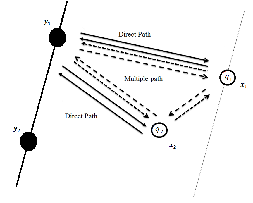
Figure 2: Four propagation paths associated with transmitted signal from sensor $\mathbf{y}_{1}$ in (IV-A).

For this two-sensor problem,

$$S=\begin{pmatrix}a&c\\ c&b\end{pmatrix}$$ (64)

where

$$a= \left(\omega^{2}\tilde{G}(\mathbf{y}_{1}-\mathbf{x}_{2})q_{2}\tilde{G}(\mathbf{x}_{2}-\mathbf{x}_{1})q_{1}\tilde{G}(\mathbf{x}_{1}-\mathbf{y}_{1})\right.$$

$$+\omega^{2}\tilde{G}(\mathbf{y}_{1}-\mathbf{x}_{1})q_{1}\tilde{G}(\mathbf{x}_{1}-\mathbf{x}_{2})q_{2}\tilde{G}(\mathbf{x}_{2}-\mathbf{y}_{1})$$

$$+\tilde{G}(\mathbf{y}_{1}-\mathbf{x}_{1})q_{1}\tilde{G}(\mathbf{x}_{1}-\mathbf{y}_{1})$$

$$\left.+\tilde{G}(\mathbf{y}_{1}-\mathbf{x}_{2})q_{2}\tilde{G}(\mathbf{x}_{2}-\mathbf{y}_{1})\right)\frac{\omega^{2}}{\xi},$$ (65)

$$b= \left(\omega^{2}\tilde{G}(\mathbf{y}_{2}-\mathbf{x}_{2})q_{2}\tilde{G}(\mathbf{x}_{2}-\mathbf{x}_{1})q_{1}\tilde{G}(\mathbf{x}_{1}-\mathbf{y}_{2})\right.$$

$$+\omega^{2}\tilde{G}(\mathbf{y}_{2}-\mathbf{x}_{1})q_{1}\tilde{G}(\mathbf{x}_{1}-\mathbf{x}_{2})q_{2}\tilde{G}(\mathbf{x}_{2}-\mathbf{y}_{2})$$

$$+\tilde{G}(\mathbf{y}_{2}-\mathbf{x}_{2})q_{2}\tilde{G}(\mathbf{x}_{2}-\mathbf{y}_{2})$$

$$\left.+\tilde{G}(\mathbf{y}_{2}-\mathbf{x}_{1})q_{1}\tilde{G}(\mathbf{x}_{1}-\mathbf{y}_{2})\right)\frac{\omega^{2}}{\xi},$$ (66)

$$c= \left(\tilde{G}(\mathbf{y}_{2}-\mathbf{x}_{1})q_{1}\omega^{2}\tilde{G}(\mathbf{x}_{1}-\mathbf{x}_{2})q_{2}\tilde{G}(\mathbf{x}_{2}-\mathbf{y}_{1})\right.$$

$$+\tilde{G}(\mathbf{y}_{2}-\mathbf{x}_{2})q_{2}\tilde{G}(\mathbf{x}_{2}-\mathbf{y}_{1})$$

$$+\tilde{G}(\mathbf{y}_{2}-\mathbf{x}_{2})q_{2}\tilde{G}(\mathbf{x}_{2}-\mathbf{x}_{1})q_{1}\omega^{2}\tilde{G}(\mathbf{x}_{1}-\mathbf{y}_{1})$$

$$\left.+\tilde{G}(\mathbf{y}_{2}-\mathbf{x}_{1})q_{1}\tilde{G}(\mathbf{x}_{1}-\mathbf{y}_{1})\right)\frac{\omega^{2}}{\xi}.$$ (67)

The derivations of these expressions are provided in Appendix C. In terms of (IV-A)-(IV-A), the trace of $L$ is

$$\mathrm{tr}(L)=\left(|a|^{2}+|b|^{2}+2|c|^{2}\right),$$ (68)

and the determinant of $L$ is

$$\det(L) =|\det(S)|^{2}=|ab-c|^{2}.$$ (69)

The eigenvalues of a $2\times 2$ matrix can be written in terms of the trace and determinant as

$$\sigma_{1,2}={\mathrm{tr}(L)\pm\sqrt{\mathrm{tr}(L)^{2}-4\det(L)}\over 2}.$$ (70)

Because the eigenvalues are real valued, tr$(L)$ and det$(L)$ must be real, and in particular the discriminant of (70) cannot be negative. Therefore, $4\det(L)/\mathrm{tr}(L)^{2}<1$. We can expand the square root in (70) and approximate both eigenvalues by their first-order terms

$$\sigma_{1} \approx\mathrm{tr}(L)-\frac{\det(L)}{\mathrm{tr}(L)}$$ (71)

$$\sigma_{2} \approx{\det(L)\over\mathrm{tr}(L)}.$$ (72)

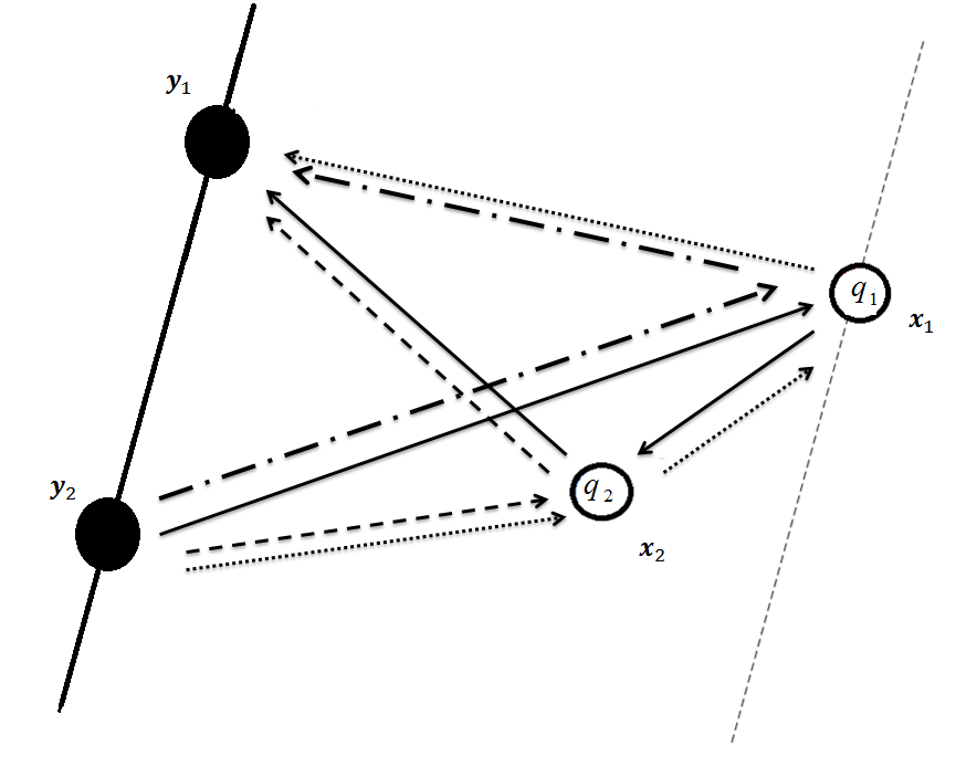
Figure 3: Propagation paths of $c$ in (IV-A) from sensor $\mathbf{y}_{2}$.

IV-B Frequency dependence of TR matrix $L$

The quantities $a$, $b$, and $c$ of (64) have physical meaning: they describe how the scatterers diffract the waves. To understand their physical interpretations, we inspect the product of $S$ with the $k^{\mathrm{th}}$ iterate of the transmitted vector in the Power Method of (59)-(61):

$$S(\omega)\tilde{\mathbf{T}}^{k}(\omega) = \left(\begin{array}[]{cc}a&c\\ c&b\end{array}\right)\left(\begin{array}[]{c}\tilde{T}^{k}_{1}(\omega)\\ \tilde{T}^{k}_{2}(\omega)\end{array}\right)$$ (77)

$$= \left(\begin{array}[]{c}a\tilde{T}^{k}_{1}(\omega)+c\tilde{T}^{k}_{2}(\omega)\\ c\tilde{T}^{k}_{1}(\omega)+b\tilde{T}^{k}_{2}(\omega)\end{array}\right).$$ (80)

Since the first component $a\tilde{T}^{k}_{1}+c\tilde{T}^{k}_{2}$ is a sum of transmitted signals from sensor $\mathbf{y}_{1}$ $(a\tilde{T}^{k}_{1})$ and sensor $\mathbf{y}_{2}$ $(c\tilde{T}^{k}_{2})$, then $a$ and $c$ are associated with the propagation paths starting from sensors $\mathbf{y}_{1}$ and $\mathbf{y}_{2}$, respectively. Similarly, for the second component $(c\tilde{T}^{k}_{1}+b\tilde{T}^{k}_{2})$, $c$ and $b$ are associated with propagation paths starting from sensor $\mathbf{y}_{1}$ $(c\tilde{T}^{k}_{1})$ and sensor $\mathbf{y}_{2}$ $(b\tilde{T}^{k}_{2})$, respectively.

As depicted in Fig. 2, the wave propagation corresponding to $a$ has four propagation paths associated with a signal that is transmitted from and received by sensor $\mathbf{y}_{1}$. The first term in $a$ describes a wave propagating from the sensor $\mathbf{y}_{1}$ to the scatterer at $\mathbf{x}_{1}$ where it scatters with strength $q_{1}$, then travels to $\mathbf{x}_{2}$ where it is scattered with strength $q_{2}$, and finally propagates from $\mathbf{x}_{2}$ to $\mathbf{y}_{1}$ $(\text{path }\mathbf{y}_{1}\to\mathbf{x}_{1}\to\mathbf{x}_{2}\to\mathbf{y}_{1})$. Similarly, the second term corresponds to the path $\mathbf{y}_{1}\to\mathbf{x}_{2}\to\mathbf{x}_{1}\to\mathbf{y}_{1}$. The third term of $a$ describes the direct-path scattering, in which the wave propagates from $\mathbf{y}_{1}$ to the scatterer at $\mathbf{x}_{1}$, where it is reflected with strength $q_{1}$ directly back to sensor $\mathbf{y}_{1}$ $(\mathbf{y}_{1}\to\mathbf{x}_{1}\to\mathbf{y}_{1})$. The fourth term describes the corresponding direct-path scattering from the scatterer at $\mathbf{x}_{2}$ back to $\mathbf{y}_{1}$ $(\mathbf{y}_{1}\to\mathbf{x}_{2}\to\mathbf{y}_{1})$. The factor $\xi$ corresponds to waves reverberating between the scatterers.

Similarly, expression $b$ represents the four paths emanating from and returning to sensor $\mathbf{y}_{2}$.

Expression $c$ has two interpretations, depending on whether the signal starts from sensor $\mathbf{y}_{1}$ or sensor $\mathbf{y}_{2}$. If the signal is transmitted from sensor $\mathbf{y}_{2}$ $(c\tilde{T}^{k}_{2})$, the first term in (IV-A) represents propagation from sensor $\mathbf{y}_{2}$ to scatterer $\mathbf{x}_{1}$ to scatterer $\mathbf{x}_{2}$ and finally to sensor $\mathbf{y}_{1}$ $(\mathbf{y}_{2}\to\mathbf{x}_{1}\to\mathbf{x}_{2}\to\mathbf{y}_{1})$. The second through fourth terms describe the remaining three paths $(\mathbf{y}_{2}\to\mathbf{x}_{2}\to\mathbf{y}_{1},\ \mathbf{y}_{2}\to\mathbf{x}_{2}\to\mathbf{x}_{1}\to\mathbf{y}_{1},\ \mathbf{y}_{2}\to\mathbf{x}_{1}\to\mathbf{y}_{1})$ in Fig. 3. Each path starts at sensor $\mathbf{y}_{2}$ and ends at sensor $\mathbf{y}_{1}$. Now if the signal is transmitted by sensor $\mathbf{y}_{1}$ $(c\tilde{T}^{k}_{1})$, the four terms in $c$ are interpreted as all possible single-scatter paths from sensor $\mathbf{y}_{1}$ to sensor $\mathbf{y}_{2}$: $\mathbf{y}_{1}\to\mathbf{x}_{2}\to\mathbf{x}_{1}\to\mathbf{y}_{2},\ \mathbf{y}_{1}\to\mathbf{x}_{2}\to\mathbf{y}_{2},\ \mathbf{y}_{1}\to\mathbf{x}_{1}\to\mathbf{x}_{2}\to\mathbf{y}_{2},\ \mathbf{y}_{1}\to\mathbf{x}_{1}\to\mathbf{y}_{2}$. We observe that these four paths are the reverse of the four paths when the signal emanates from sensor $\mathbf{y}_{2}$.

The largest eigenvalue of the TR operator $L$ in (71) represents the contribution of all the wave interactions that occur in the medium measured at the sensor locations. The maximum value for the eigenvalue $\sigma_{1}$ of $L$ occurs when the waves described in $a$, $b$, and $c$ all constructively add. This occurs when the path differences between every pair of propagation paths are equal to integer multiples of some fundamental wavelength $\lambda_{0}$. From the many redundant equations corresponding to this constructive addition condition, only the following three relations are needed to specify that all waves add constructively.

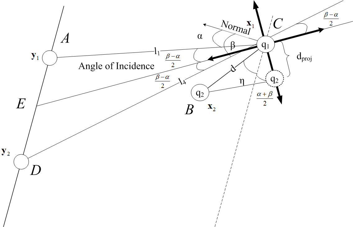
Figure 4: Geometry of the distributed sensors and scatterers $d<<l_{k}$, $l_{k}\to\infty$. Farfield approximation of Figure 1 using $\mathbf{x}_{1}$ as the reference scatterer. As the distance of the sensors and scatterers increases, $l_{1}\approx l_{4}\approx l$ and $l_{2}\approx l_{3}$ in Figure 1 result in the bisection of subtending angle by the segment connecting the midsection between the sensors to the reference scatterer.

1. From Figure 1, we see that the difference between the direct-path scattering $\mathbf{y}_{1}\longleftrightarrow\mathbf{x}_{2}$ and the path $\mathbf{y}_{1}\to\mathbf{x}_{2}\to\mathbf{x}_{1}\to\mathbf{y}_{1}$ must be an integer multiple of the wavelength $\lambda_{0}$:

   $${2l_{3}-(l_{3}+d+l_{1})\over\lambda_{0}}={l_{3}-d-l_{1}\over\lambda_{0}}=m,$$ (81)

   where $m$ is an integer.

2. The path difference between the direct-path scattering $\mathbf{y}_{2}\longleftrightarrow\mathbf{x}_{1}$ and the path $\mathbf{y}_{2}\to\mathbf{x}_{2}\to\mathbf{x}_{1}\to\mathbf{y}_{2}$, must be an integer multiple of the wavelength:

   $${2l_{4}-(l_{2}+d+l_{4})\over\lambda_{0}}={l_{4}-d-l_{2}\over\lambda_{0}}=p,$$ (82)

   where $p$ is an integer.

3. The path difference between paths $\mathbf{y_{2}}\to\mathbf{x}_{2}\to\mathbf{y}_{1}$ and $\mathbf{y_{2}}\to\mathbf{x}_{1}\to\mathbf{x}_{2}\to\mathbf{y}_{1}$ must be an integer multiple of the wavelength:

   $${l_{2}+l_{3}-(l_{4}+d+l_{3})\over\lambda_{0}}={l_{2}-l_{4}-d\over\lambda_{0}}=r,$$ (83)

   where $r$ is an integer.

To obtain a single equation that involves the four propagation distances $\{l_{1},l_{2},l_{3},l_{4}\}$, we add (83) and (82) to get $-2d/\lambda_{0}=p+r$, and substitute this result into sum of (81) and (82). Consequently,

$${l_{3}+l_{4}-l_{1}-l_{2}\over\lambda_{0}}=m+p-(p+r)=n,$$ (84)

where $n$ is an integer. By the law of sines,

$$l_{1} = {d\sin\zeta\over\sin\theta}$$ (85)

$$l_{2} = {d\sin(\phi+\psi)\over\sin\phi}$$ (86)

$$l_{3} = {d\sin(\zeta+\theta)\over\sin\theta}$$ (87)

$$l_{4} = {d\sin\psi\over\sin\phi},$$ (88)

which represent each $l_{k}$ in terms of $d$ and various incident angles in Fig. 1. After some manipulation (Appendix D), Equation (84) becomes

$$(l_{4}-l_{2})+ (l_{3}-l_{1})=d\left({\sin\psi-\sin(\phi+\psi)\over\sin\phi}\right.$$

$$+\left.{\sin(\zeta+\theta)-\sin\zeta\over\sin\theta}\right)=n\lambda_{0},$$ (89)

which is Bragg’s condition for constructive interference [27, pp. 706-707]. As the distances from the sensors to the scatterers approach infinity, $l_{k}\to\infty$, which implies that $\theta\to 0$, $\phi\to 0$, and $(\beta-\alpha)/2$ bisects the angle subtended by vectors from $\mathbf{x}_{1}$ to the two sensors. In the far-field limit, (IV-B) becomes (see Appendix D for the proof)

$$n\lambda_{0} \approx d(-\cos\psi+\cos\zeta)$$

$$\approx d\left(\sin(\eta+\beta)-\sin(\eta+\alpha)\right)$$

$$=2d\cos\left(\eta+{\alpha+\beta\over 2}\right)\sin\left({\beta-\alpha\over 2}\right).$$ (90)

Equation (IV-B) can be understood in terms of Bragg’s Law with the help of Fig. 4, where the four thick axis vectors in Fig. 4 define a relevant reference frame. The angle between the axis vector from $C$ to the sensor midpoint $E$ and the “normal” is $(\alpha+\beta)/2$. This angle, when rotated by $90^{\circ}$, is the angle in Fig. 4 labelled $(\alpha+\beta)/2$. Consequently, Bragg’s Law is

$$2d_{\mathrm{proj}}\sin\left({\beta-\alpha\over 2}\right)\approx n\lambda_{0}$$ (91)

where $d_{\mathrm{proj}}=d\cos\left(\eta+\frac{\alpha+\beta}{2}\right)$ is the projection of $d$ onto the line perpendicular to the bisecting vector.

From the preceding analysis, Bragg’s Law also gives the frequencies at which the largest eigenvalue $\sigma_{1}$ of the TR matrix $L$ achieves a maximum. This largest $\sigma_{1}$ is the maximum field intensity at both sensors. The smaller eigenvalue $\sigma_{2}$ in (72) is the ratio of the determinant and the trace of $L$. From (69), the determinant is $|ab-c|^{2}$. The quantities $a$ and $b$ correspond to propagation paths beginning and ending at $\mathbf{y}_{1}$ and $\mathbf{y}_{2}$, respectively. Since $c$, which corresponds to propagation paths that begin at one sensor and end at the other, is subtracted from $ab$, the determinant of $L$ in (69) can be interpreted as the contribution from the destructive interference of the received fields at both sensors. We now discuss the relationship between the two eigenvalues.

V Connection to SEM

Carl Baum first introduced SEM in the context of electromagnetic scatterers and antennas [28, 20]. His approach to modeling the scattered field in terms of poles was originally motivated by the observation of typical transient responses of complex scatterers. He conjectured that the responses were dominated by several damped sinusoids, and his main focus was scatterers on which the incident field creates surface current densities. These densities can be analyzed in terms of the object’s natural frequencies $\omega_{\alpha}$ [20], which typically occur at complex (non-physical) values.

In particular, each component of the scattering matrix $S$ is a meromorphic function of $\omega$, where the poles $\{\omega_{\alpha_{k}}\}_{k=1}^{\infty}$ satisfy $\xi=1-q_{1}q_{2}\omega_{\alpha_{k}}^{4}\tilde{G}^{2}(\mathbf{d},\omega_{\alpha_{k}})=0$ and are put in order of increasing imaginary part. Each element of the scattering matrix can be expanded in a Laurent series for $S(\omega)$ around a given pole $\omega_{\alpha_{k}}$

$$S(\omega)=\sum\limits_{n=-m}^{\infty}s_{n}(\omega-\omega_{\alpha_{k}})^{n},$$ (92)

where $m$ is a positive integer, and $s_{n}$ is a matrix of the residues of the element of $S(\omega)$ at $\omega_{\alpha_{k}}$.

When the transmitted waveform $\tilde{\mathbf{T}}(\omega)$ is analytic, then $\tilde{\mathbf{R}}(\omega)$ is meromorphic. Moreover, both $\mathbf{T}(t)$ and $\mathbf{R}(t)$ must be causal ($\mathbf{T}(t)=\mathbf{0}=\mathbf{R}(t)$ for $t<0$). By the Paley-Wiener theorem [29, p. 494], both $\tilde{\mathbf{T}}(\omega)$ and $\tilde{\mathbf{R}}(\omega)$ are then analytic in the lower half-plane. Consequently the poles of the $\tilde{\mathbf{R}}(\omega)$ must lie in the upper half plane. Using the Paley-Wiener Theorem allows one to avoid the convergence issues inherent in Baum’s Laplace formulation.

To predict the time-domain received signal, we must compute the inverse Fourier transform (4) for the received signal, which may require modification of the integration contour. By an appropriate contour deformation and residue calculus,

$$\mathbf{R}(t)\approx 2\pi j\sum\limits_{i=1}^{N} \underset{\omega=\omega_{\alpha_{i}}}{\mathrm{Res}}\left(\frac{\mathbf{\tilde{R}}(\omega)e^{j\omega t}}{2\pi}\right)$$

$$+O(e^{-|\mathrm{Im}(\omega_{\alpha_{N}})|t}),$$ (93)

where the higher-order terms vanish as $t\to\infty$, and the notation $f(x)=O(g(x))$ means that $|f(x)|\leq M|g(x)|$ for some positive real number $M$ as $x\to\infty$. Equation (V) is the SEM representation of the transient backscattered response at the receivers [28, 30].

We note that the poles due to $\xi$ are a result of the interaction between the fields and scatterers. These poles are aspect independent, and it is for this reason that they have been proposed for use in target classification [31]. Consequently, a number of methods, such as the Matrix Pencil Method and Prony’s Method, have been developed for determining these poles [32, 33, 34, 35, 36]. Unfortunately, the problem of obtaining these poles from real data is ill-posed and sensitive to noise.

Previous research [37, 38] has shown, however, that there is a connection between the eigenvalues of the scattering matrix and the complex poles used for Baum’s SEM. Although the SEM poles are aspect-independent, unfortunately the scattering matrix itself and consequently the received signals are aspect-dependent.

We show below that the TR matrix can be used to obtain certain information about the poles of $S$ in a stable manner. First, we introduce the notation $\hat{S}$:

$$S=\frac{\omega^{2}}{\xi}P\Delta P^{T}=\frac{\omega^{2}}{\xi}\hat{S},$$ (94)

where $\hat{S}=P\Delta P^{T}$ and

$$\det(\hat{S}(\omega))=\det(P(\omega))\underbrace{\det(\Delta(\omega))}_{q_{1}q_{2}\xi(\omega)}\det(P^{T}(\omega)).$$ (95)

The corresponding modified TR matrix $\hat{L}$ is

$$\hat{L}=\hat{S}^{\dagger}\hat{S},\quad L=\left|\frac{\omega^{2}}{\xi}\right|^{2}\hat{L}.$$ (96)

From (38), at a natural frequency $\omega=\omega_{\alpha}$, we have $\xi(\omega_{\alpha})=0$; from (95) we see that the determinant of $\hat{S}$ and therefore also of $\hat{L}$ must be zero, implying that at least one of the eigenvalues of $\hat{S}$ and $\hat{L}$ must be 0. As $\omega\to\omega_{\alpha}$ and $\xi\to 0$, the eigenvalues of the interaction matrix $\Delta$ can be approximated from (39) by

$$\lim\limits_{\omega\to\omega_{\alpha}}\lambda_{1}(\omega) \approx q_{1}+q_{2},$$ (97)

$$\lim\limits_{\omega\to\omega_{\alpha}}\lambda_{2}(\omega) \approx \frac{q_{1}q_{2}}{q_{1}+q_{2}}\xi,$$ (98)

where the derivation of (98) is in Appendix E. From (A) in Appendix A, the eigenvalues of $S$ behave as

$$\lim\limits_{\omega\to\omega_{\alpha}}\gamma_{1}(\omega) \approx\lim\limits_{\omega\to\omega_{\alpha}}\frac{\omega^{2}}{\xi}\lambda_{1}m_{11}$$

$$=\frac{\omega_{\alpha}^{2}}{\xi}(q_{1}+q_{2})m_{11},$$ (99)

$$\lim\limits_{\omega\to\omega_{\alpha}}\gamma_{2}(\omega) \approx\lim\limits_{\omega\to\omega_{\alpha}}\frac{\omega^{2}}{\xi}\lambda_{2}m_{22}$$

$$=\frac{\omega_{\alpha}^{2}q_{1}q_{2}}{q_{1}+q_{2}}m_{22}.$$ (100)

Clearly, $\gamma_{1}$ diverges as $\xi\to 0$, while $\gamma_{2}$ converges to $\omega_{\alpha}^{2}q_{1}q_{2}m_{22}/(q_{1}+q_{2})$ .

We determine the eigenvalues of the TR matrix $L$ from $\{\gamma_{1},\gamma_{2}\}$ by (123) in Appendix B. Consequently, the eigenvalues of $L$ behave as

$$\lim\limits_{\omega\to\omega_{\alpha}}\sigma_{1} =\left(\frac{\omega_{\alpha}^{2}}{\xi}(q_{1}+q_{2})m_{11}\frac{(\mathbf{v}_{1}^{*},\mathbf{y}_{1})}{(\mathbf{v}_{1},\mathbf{y}_{1})}\right)^{2},$$ (101)

$$\lim\limits_{\omega\to\omega_{\alpha}}\sigma_{2} =\left(\frac{\omega_{\alpha}^{2}q_{1}q_{2}m_{22}(\mathbf{v}_{2}^{*},\mathbf{y}_{2})}{(q_{1}+u_{2})(\mathbf{v}_{2},\mathbf{y}_{2})}\right)^{2},$$ (102)

where $\mathbf{v}_{i}$ is an eigenvector of $L$ for $\sigma_{i}$ and $\mathbf{y}_{i}$ is an eigenvector of $S$ for $\gamma_{i}$. Clearly, the larger eigenvalue of $L$ diverges to positive infinity in the limit $\omega\to\omega_{\alpha}$, while smaller eigenvalue $\sigma_{2}$ converges to a finite number. Because in general the natural frequencies $\omega_{\alpha_{k}}$ are complex-valued, the larger eigenvalue does not actually diverge for real frequencies, and instead one sees resonance peaks.

When the damping is small ($\mathrm{Im}(\omega_{\alpha})<<1$), the real resonant frequency is approximately equal to the complex natural frequency, and we will expect a significant response at this frequency. The difference between a real resonant frequency $\omega_{\alpha}$ and its associated complex natural frequency depends on the phase of $\omega_{\alpha}$.

Thus the TR algorithm provides information about the rotation of the natural frequencies $\omega_{\alpha_{k}}$ onto the real axis. Moreover, we show in the next section that this information can be obtained in a stable manner. Therefore, the TR algorithm provides a stable way of obtaining information about the SEM poles.

VI Stability of Eigenvalues

In this section, we compare and contrast the eigenvalues of $S$ and $L$ and show how these eigenvalues are respectively perturbed by noise.

VI-A Stability of finding eigenvalues from measurements of $S$

Thermal noise gives rise to perturbations in the elements of the scattering matrix. We would like to examine how a small change $\delta S$ in the scattering matrix is translated to the changes $\delta\Gamma$ in the eigenvalues of $S$. We re-write (49) as

$$Y^{-1}SY=\Gamma.$$ (103)

Inserting $\Gamma+\delta\Gamma$ and $S+\delta S$ into (103) and rearranging, we have

$$\delta\Gamma=Y^{-1}\delta SY.$$ (104)

Taking the operator norm $\|\cdot\|$ and applying a standard matrix product inequality yields

$$\|\delta\Gamma\|=\|Y^{-1}\delta SY\|\leq\|Y^{-1}\|\|\delta S\|\|Y\|.$$ (105)

The error is then bounded by

$$\max_{\omega}\|\delta\Gamma\|\leq\|Y^{-1}\|\|Y\|\|\delta S\|=\max_{\omega}\>\kappa(Y)\|\delta S\|,$$ (106)

where $\kappa$ is the condition number. The errors in the eigenvalues are thus bounded by the errors in measurement introduced in $S$ and the conditioning of the eigenvectors of $S$ (columns of $Y$). Since $Y$ depends on the field propagation paths and scattering, the conditioning will be a function of the configuration of the transmitters, receivers, scatterers, and the frequency. In general, finding the eigenvalues of $S$ from measurements of $S$ is an unstable process.

VI-B Stability of finding eigenvalues from TR measurements

For the TR operator, the errors in the eigenvalues are less subject to the configuration of the system. From (63),

$$\max_{\omega}\|\delta\Sigma\|\leq\|V\|\|V^{\dagger}\|\|\delta L\|.$$ (107)

Since $V$ is unitary, the norms are both $1$, and

$$\max_{\omega}\|\delta\Sigma\|\leq\max_{\omega}\|\delta L\|.$$ (108)

The error in the eigenvalues of $L$ is bounded by the error introduced in the measurement and does not rely on the conditioning of $Y$. The error bound in (108) suggests that finding the eigenvalues of the TR operator is a more well-conditioned problem than finding the eigenvalues of the scattering operator and may provide a stable way of calculating the eigenvalues of the scattering operator.

VII Numerical Results

In this section, we provide simulations of the TR algorithm for two transmitter/receiver pairs and two isotropic scatterers in free space. The two transmit/receive pairs are placed at coordinates (-500 m, 700 m, 10 m) and (-500 m, 1000 m, 10 m). The scatterers are separated by 500 m, with the strong one $(q_{1})$ located at (150 m, 850 m, 10 m) and the weaker one $(q_{2})$ located at (-107.52 m, 1278.58 m, 10 m). In addition, the transmitter/receiver pairs and the scatterers are placed in a plane with $q_{1}=0.75\>\mathrm{Hz}^{-2}\mathrm{m}^{-2}$ and $q_{2}=0.4\>\mathrm{Hz}^{-2}\mathrm{m}^{-2}$. The initial waveform $T^{0}(t)$ for each transmitter is the same linear frequency modulated (LFM) signal with the following characteristics:

1. $10\>\mu\mathrm{s}$ pulse duration;

2. $10^{12}\>\mathrm{s}^{-2}$ chirp rate;

3. $100\>\mathrm{MHz}$ carrier frequency.

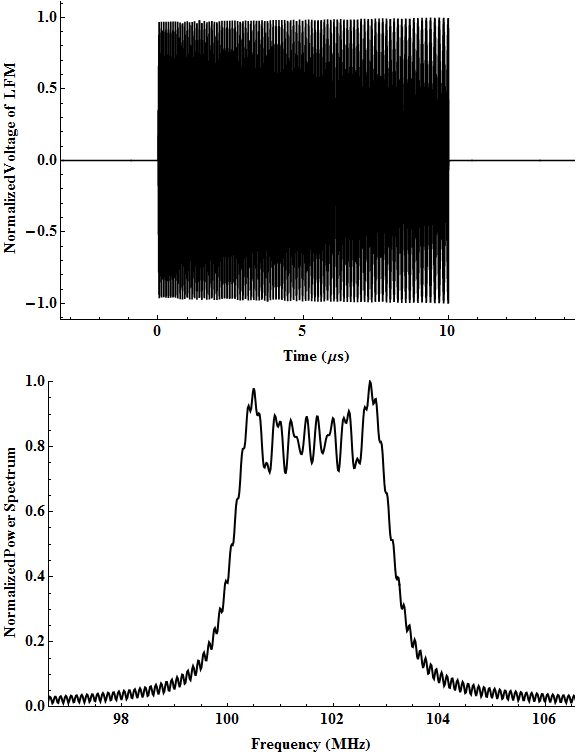
Figure 5: Original LFM Signal $T^{0}$: time-domain signal (top); square magnitude of power spectrum (bottom) with 4 MHz bandwidth centered at 100 MHz.

For the simulations, we limit ourselves to the even iterations of the transmitted signal. We normalize the signal vector with the euclidean norm for each iteration. We observe the transformation of the original chirp to the final waveform in the time domain and the power spectrum of the signal.

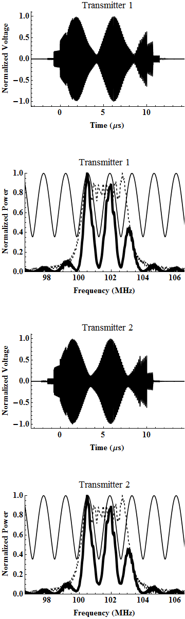
Figure 6: Top two rows show the normalized transmitted waveform and the power spectrum of sensor 1 after two iterations of the TR algorithm. Bottom two rows show the normalized transmitted waveform and power spectrum of sensor 2 after two iterations. The original LFM (dotted line), the normalized power spectrum of the signal (thick line), and the normalized calculated eigenvalues (thin line) are shown. Scatterers are 500m apart.

Figure 6 shows the final waveform from $T^{0}$ after 2 iterations of the TR process, the normalized magnitude of the spectra for TR-generated signals, and the normalized calculated eigenvalues of $L$ for a scatterer separation of 500 m. As the figure indicates, the time-domain waveform significantly changes and broadens from the original LFM signal for both transmitters. The power spectrum of each new waveform has relative maximum values at the resonant frequencies. Observe that for a given bandwidth of the original LFM signal, the energy of the TR-generated signals after 2 iterations (thick line) concentrates near the resonant frequencies. Significantly, the maxima of this power spectrum aligns with the maxima of the calculated eigenvalues of the TR operator (thin line). The peaks of the power spectrum occur within the bandwidth of the power spectrum of $T^{0}$ (dashed curve).

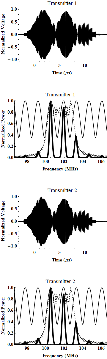
Figure 7: Top two rows show the normalized transmitted waveform and the power spectrum of sensor 1 after ten iterations of the TR algorithm. Bottom two rows show the normalized transmitted waveform and power spectrum of sensor 2 after ten iterations. The original LFM (dotted line), the normalized power spectrum of the signal (thick line), and the normalized calculated eigenvalues (thin line) are shown. Scatterers are 500m apart.

At higher iterations of the TR process, the field intensities increase at the resonant frequencies and decrease at other frequencies.. In particular, Fig. 7 plots the power spectrum and the time-domain signal at 10 iterations. The frequency peaks are sharp, and one can observe the key resonating frequency where the intensity is at its highest. The time-domain waveform has broadened from the $10\>\mu s$ pulse in Fig. 5 as the new waveform is determined by the resonant frequencies. The plot of the power of the original LFM signal is now narrowed and centered around the resonant frequencies. The largest intensity is found within the bandwidth of the original signal.

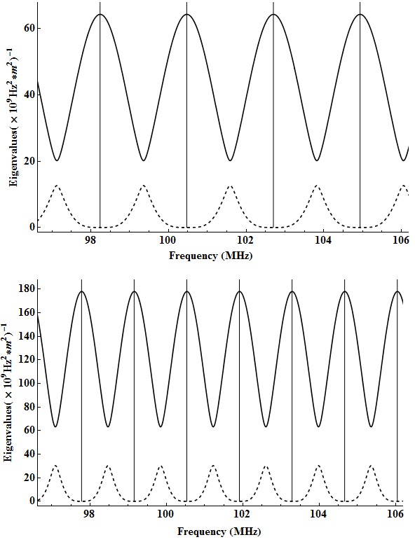
Figure 8: First and second eigenvalues of the TR matrix $L$ are shown at two separate distances of the point scatterers, 300 m (top) and 500 m (bottom) respectively with the transmitter and stronger scatterer in the same position. The two figures shown are the theoretical eigenvalues – larger eigenvalue (solid), smaller eigenvalue (dashed), and the vertical line indicates the Bragg frequencies.

Figure 8 shows the large and small eigenvalues. As discussed in Section V, the larger eigenvalues attain relative maximum values at resonance. The vertical lines indicate the frequency at which Bragg’s condition is met. Maximum constructive interference occurs at these frequencies and matches the eigenvalue peaks which are $1.37$ MHz apart. This frequency separation corresponds to the projected distance between the scatterers, where the projection is onto the axis normal to the axis vector from the strong scatterers to the midpoint of the sensors ($d_{\mathrm{p}roj}$ in Fig. 4). In this case, the actual distance between the scatterers is $500$ m ($=$$d$), and the projected distance is $484$ m. For both scatterer separations in Fig. 8, the larger eigenvalue has a maximum at the resonance frequencies. The locations of the resonances (vertical lines) are exact because the formula for Bragg’s Law (a geometric approximation) is not used. However, when Bragg’s Law is used, the vertical lines will be slightly displaced from the relative maxima due to the geometrical approximation introduced in deriving the Bragg’s formula in Appendix D. This displacement error can be explained by modifying the analysis treated in [39].

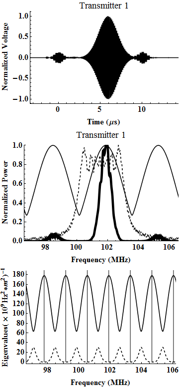
Figure 9: The scatterers rotated $81^{\circ}$ in azimuth from the initial configuration. $d$ remains the same. The eigenvalue peaks are $3.39$ MHz apart. TR process was taken out to 10 iterations. Top row is the time-domain signal; middle row is the power spectrum, bottom row is the first (solid line) and second eigenvalues (dashed line) of the TR matrix.

In Figure 9, the weaker scatterer is rotated $81^{\circ}$ in azimuth about the stronger scatterer from the original configuration. The projected distance is $197$ m. The scatterer separation distance of $500$ m remains the same, but the separation between frequency peaks changes to 3.39 MHz. As the projected distance decreases, the eigenvalue peaks will be further apart. A signal with a broader bandwidth will be required to observe multiple resonant peaks. Thus the aspect angle, which determines the propagation paths of the fields, has a strong influence on the locations of the eigenvalue peaks.

VIII Conclusions

We have shown that in a multiple-scattering environment, the TR matrix has eigenvalues that vary with frequency in ways that can be predicted by the interaction of the scattered waves. In contrast to the case of non-interacting scatterers [26, 10] where different eigenvalues correspond to different scatterers, we have shown that when multiple scattering is present, each eigenvalue involves the field interactions from all the propagation paths and all the scatterers. The largest eigenvalue can be thought of as corresponding to the field intensities at the receivers from all the scattered waves. The frequencies at which the largest eigenvalue has local maxima are the resonance frequencies, where maximum constructive interference occurs, and the frequency difference between the peaks depends on the wavelength and geometry of the scatterers.

Our work shows that the TR process provides a stable way of finding the resonances of a scattering system. Moreover, the TR process can be applied to an arbitrary waveform of arbitrary bandwidth. Our work confirms the findings of [17, 16], which showed, for an idealized half-space scattering geometry, the TR algorithm automatically converges to the space-time waveform that maximizes the energy scattered back to the receivers. Our work shows that the same result holds for a more realistic scattering geometry. Thus the best waveform for target detection is a single harmonic waveform at one of the resonance frequencies, and the TR process provides a stable method to find these resonance frequencies.

We have shown, moreover, that these scattering system resonances are closely related to the poles of the SEM. In particular, as the poles of the SEM approach the real axis, the SEM poles become exactly the resonances found by the TR process. The precise nature of the information about the SEM poles that is provided by the TR process is a question we leave for future work.

Appendix A Derivation of the eigenvalues of the Scattering Matrix $S$

The characteristic polynomial of (53) using (54) can be expressed as

$$\det\left(\frac{\omega^{2}}{\xi}\Lambda M-\gamma I\right)=0,$$ (109)

$$\Lambda=\left[\begin{array}[]{cc}\lambda_{1}&0\\ 0&\lambda_{2}\end{array}\right],\quad M=\left[\begin{array}[]{cc}m_{11}&m_{12}\\ m_{21}&m_{22}\end{array}\right],$$ (110)

which after substitution of (110) becomes

$$\det\left(\left[\begin{array}[]{cc}\frac{\omega^{2}}{\xi}\lambda_{1}m_{11}-\gamma&\frac{\omega^{2}}{\xi}\lambda_{1}m_{12}\\ \frac{\omega^{2}}{\xi}\lambda_{2}m_{21}&\frac{\omega^{2}}{\xi}\lambda_{2}m_{22}-\gamma\end{array}\right]\right)=0.$$ (111)

Since the matrix is $2\times 2$, the solution to (111) can be expressed in terms of the trace and determinant of $\Lambda M$:

$$\gamma=\frac{\omega^{2}}{\xi}\frac{\mathrm{tr}(\Lambda M)\pm\sqrt{\mathrm{tr}(\Lambda M)^{2}-4\det(\Lambda M)}}{2},$$ (112)

where

$$\mathrm{tr}(\Lambda M) = \lambda_{1}m_{11}+\lambda_{2}m_{22}$$

$$\det(\Lambda M) = \lambda_{1}\lambda_{2}m_{11}m_{22}-\lambda_{1}\lambda_{2}m_{12}m_{21}.$$

From (54), $m_{ip}$ can be written in index form as

$$m_{ip}=\sum\limits_{n=1}^{2}\sum\limits_{k=1}^{2}\sum\limits_{l=1}^{2}X_{in}^{-1}P_{kn}P_{kl},X_{lp},$$ (113)

and

$$\gamma_{1,2} =\frac{\omega^{2}}{\xi}\times\left(\frac{\lambda_{1}m_{11}+\lambda_{2}m_{22}}{2}\right.$$

$$\left.{\pm\sqrt{(\lambda_{1}m_{11}-\lambda_{2}m_{22})^{2}+4\lambda_{1}\lambda_{2}m_{21}m_{12}}\over 2}\right).$$ (114)

Appendix B Relationship between Singular Values of the Scattering Operator $S$ and the Eigenvalues of the TR Operator $L$

Any matrix $S$ has a singular value decomposition

$$S=U\Sigma V^{\dagger},$$ (115)

where $U$ and $V$ are unitary matrices. If we multiply (115) by the adjoint $S^{\dagger}$, then we have

$$L=S^{\dagger}S = V\Sigma^{\dagger}U^{\dagger}U\Sigma V^{\dagger}$$ (116)

$$= V\Sigma^{2}V^{\dagger},$$ (117)

and then post multiplying $V$ on both sides implies

$$S^{\dagger}SV=V\Sigma^{2}.$$ (118)

Therefore, the right singular vectors of $S$ are the eigenvectors of $L=S^{\dagger}S$, and the eigenvalues $\{\sigma_{1},\sigma_{2}\}$ of $L$ are the squares of the corresponding singular values $\{\zeta_{1},\zeta_{2}\}$ of $S$.

For a square matrix with distinct singular values, the left and right singular vectors are unique up to a complex sign (i.e., complex scalar factors of absolute value unity) [40, p. 29]. Since $S$ is square and symmetric but not self-adjoint, the left singular vectors are the conjugates of the right singular vectors:

$$V^{*}\Sigma U^{T}=S^{T}=S=U\Sigma V^{\dagger}.$$ (119)

Therefore $U=V^{*}$, which implies that for any right singular vector $\mathbf{v}_{l}$, there is a left singular vector $\mathbf{u}_{l}$ such that

$$S\mathbf{v}_{l}=\zeta_{l}\mathbf{u}_{l}=\zeta_{l}\mathbf{v}_{l}^{*}.$$ (120)

The inner product of $L\mathbf{v}_{l}$ with an eigenvector $\mathbf{y}_{n}$ of $S$ corresponding to the eigenvalue $\gamma_{n}$ is

$$\sigma_{l}(\mathbf{v}_{l},\mathbf{y}_{n}) =(L\mathbf{v}_{l},\mathbf{y}_{n})=(S^{\dagger}S\mathbf{v}_{l},\mathbf{y}_{n})=(S\mathbf{v}_{l},S\mathbf{y}_{n})$$ (121)

where $\zeta_{l}^{2}=\sigma_{l}$. In (121), we use expression (120) for $S\mathbf{v}_{l}$ and the relation $S\mathbf{y}_{n}=\gamma_{n}\mathbf{y}_{n}$ to obtain

$$\sigma_{l}(\mathbf{v}_{l},\mathbf{y}_{n})=\zeta_{l}\gamma_{n}(\mathbf{v}_{l}^{*},\mathbf{y}_{n}).$$ (122)

Since $\sqrt{\sigma_{l}}=\zeta_{l}$,

$$\sqrt{\sigma_{l}}=\gamma_{n}\frac{(\mathbf{v}_{l}^{*},\mathbf{y}_{n})}{(\mathbf{v}_{l},\mathbf{y}_{n})}.$$ (123)

Appendix C Derivation of the TR matrix $L$

We recall the definitions (94), (37), and (36) of $\hat{S}$, the propagation matrix $P$, and the interaction matrix, together with the relation $\hat{S}=P\Delta P^{T}$ between them. Then in index form,

$$\hat{S}_{ij}=\sum_{k}\sum_{l}P_{ik}\Delta_{kl}P_{jl}.$$ (124)

The corresponding modified TR matrix, which is given by (96), is

$$\hat{L}_{mj}=\sum_{i}\hat{S}^{*}_{im}\hat{S}_{ij}.$$ (125)

The trace of $\hat{L}$ is

$$\mathrm{tr}(\hat{L})=\hat{L}_{11}+\hat{L}_{22},$$ (126)

where

$$\hat{L}_{11} = \sum_{i}\hat{S}^{*}_{i1}\hat{S}_{i1},$$ (127)

$$\hat{L}_{22} = \sum_{i}\hat{S}^{*}_{i2}\hat{S}_{i2}.$$ (128)

The elements of $S$ using (124) are

$$\hat{S}_{11}=P_{11}\Delta_{11}P_{11} +P_{11}\Delta_{12}P_{12}+P_{12}\Delta_{21}P_{11}$$

$$+P_{12}\Delta_{22}P_{12},$$ (129)

$$\hat{S}_{22}=P_{21}\Delta_{11}P_{21} +P_{21}\Delta_{12}P_{22}+P_{22}\Delta_{21}P_{21}$$

$$+P_{22}\Delta_{22}P_{22},$$ (130)

$$\hat{S}_{12}=P_{11}\Delta_{11}P_{21} +P_{11}\Delta_{12}P_{22}+P_{12}\Delta_{21}P_{21}$$

$$+P_{12}\Delta_{22}P_{22},$$ (131)

$$\hat{S}_{21}=P_{21}\Delta_{11}P_{11} +P_{21}\Delta_{12}P_{12}+P_{22}\Delta_{21}P_{11}$$

$$+P_{22}\Delta_{22}P_{12},$$ (132)

which gives (64), (IV-A), (IV-A), and (IV-A). The elements of the TR matrix are then

$$L_{11} = |S_{11}|^{2}+|S_{21}|^{2}=|a|^{2}+|c|^{2}$$ (133)

$$L_{22} = |S_{22}|^{2}+|S_{12}|^{2}=|b|^{2}+|c|^{2}$$ (134)

$$L_{12} = S_{11}^{*}S_{12}+S_{21}^{*}S_{22}=a^{*}c+c^{*}b$$ (135)

$$L_{21} = S_{12}^{*}S_{11}+S_{22}^{*}S_{21}=c^{*}a+b^{*}c.$$ (136)

Appendix D Derivation of Bragg’s Formula

From Figure 1, $\triangle ABC$ and the law of sines yield

$$\frac{\sin\zeta}{l_{1}} = \frac{\sin\theta}{d},$$ (137)

$$\frac{\sin\theta}{d} = \frac{\sin\angle ACB}{l_{3}},$$ (138)

and $\angle ACB=\pi-\theta-\zeta$. Substituting this angle into (138), we obtain

$$\frac{\sin\theta}{d} = \frac{\sin(\theta+\zeta)}{l_{3}}.$$ (139)

For $\triangle DBC$,

$$\frac{\sin\phi}{d} = \frac{\sin\psi}{l_{4}},$$ (140)

$$\frac{\sin\phi}{d} = \frac{\sin\angle DCB}{l_{2}},$$ (141)

and $\angle DCB=\pi-\phi-\psi$. Substituting this angle into (141), we obtain

$$\frac{\sin\phi}{d} = \frac{\sin(\phi+\psi)}{l_{2}}.$$ (142)

These equations lead to (85), (86), (87), and (88). For $\triangle ABC$, the law of cosines yields

$$\frac{l_{1}^{2}+l_{3}^{2}-d^{2}}{2l_{1}l_{3}}=\cos\theta.$$ (143)

As $l_{1}\to\infty,l_{3}\to\infty$, $\cos\theta\to 1$, and $\theta\to 0$, the second term of (IV-B) is

$$\lim\limits_{\theta\to 0}\frac{\sin(\zeta+\theta)-\sin\zeta}{\sin\theta}=\cos\zeta.$$ (144)

For the first term of (IV-B), we look at $\triangle DBC$: from the law of cosines we have

$$\frac{l_{2}^{2}+l_{4}^{2}-d^{2}}{2l_{2}l_{4}}=\cos\phi.$$ (145)

As $l_{2}\to\infty,l_{4}\to\infty$, $\cos\phi\to 1$, and $\phi\to 0$, the first term of (IV-B) has the limit

$$\lim\limits_{\phi\to 0}\frac{\sin\psi-\sin(\phi+\psi)}{\sin\phi}=-\cos\psi.$$ (146)

When the sensors are far from the scatterers, (IV-B) can be approximated as

$$d(-\cos\psi+\cos\zeta)=q\lambda_{\text{wave}}.$$ (147)

Moreover, since the sum of the interior angles of the triangle $\triangle DBC$ must be $\pi$, and the sum of the unmarked angle of $\triangle DBC$ plus $\eta$ plus $\beta$ must be $\pi/2$, and recalling that $\phi\approx 0$, we have

$$\psi = \frac{\pi}{2}+\eta+\beta.$$ (148)

Similarly, we have

$$\zeta = \frac{\pi}{2}+\alpha+\eta.$$ (149)

In the far field, trigonometric identities can be used to rewrite (147) as (IV-B).

Appendix E Derivation of (98)

In (39) we use (31) to replace $q_{1}q_{2}\omega^{4}\tilde{G}^{2}(d,\omega)$:

$$\lambda_{2} ={1\over 2}\left[q_{1}+q_{2}-\sqrt{(q_{1}-q_{2})^{2}+4q_{1}q_{2}(1-\xi)}\right]$$ (150)

$$={1\over 2}\left[q_{1}+q_{2}-\sqrt{(q_{1}+q_{2})^{2}-4q_{1}q_{2}\xi}\right]$$ (151)

$$={1\over 2}\left[q_{1}+q_{2}-(q_{1}+q_{2})\right.$$ (152)

$$\hskip 71.13188pt\times\left.\left(1-{1\over 2}{4q_{1}q_{2}\xi\over(q_{1}+q_{2})^{2}}+\cdots\right)\right]$$ (153)

$$={q_{1}q_{2}\xi\over q_{1}+q_{2}}+O\left(\frac{q_{1}^{2}q_{2}^{2}\xi^{2}}{(q_{1}+q_{2})^{3}}\right)$$ (154)

References

- [1] V. Gregers-Hansen, “A sequential logic for improving signal detectability in frequency-agile search radars,” IEEE Trans. Aerosp. Electron. Syst., vol. AES-4, no. 5, pp. 763–773, September 1968.
- [2] M. Fink, “Time reversal of ultrasonic fields. i. basic principles,” IEEE Trans. Ultrason., Ferroelect., Freq. Control, vol. 39, no. 5, pp. 555–566, September 1992.
- [3] M. Fink and C. Prada, “Acoustic time-reversal mirrors,” Inverse Probl, vol. 17, pp. R1–R38, 2001.
- [4] W. M. G. Dyab, T. K. Sarkar, A. Garcia-Lampérez, M. Salazar-Palma, and M. A. Lagunas, “A critical look at the principles of electromagnetic time reversal and its consequences,” IEEE Antennas Propag. Mag., vol. 55, no. 5, pp. 28–62, October 2013.
- [5] J. de Rosny, G. Lerosey, and M. Fink, “Theory of electromagnetic time-reversal mirrors,” IEEE Trans. Antennas Propag., vol. 58, no. 10, pp. 3139–3149, October 2010.
- [6] B. P. Bogert, “Demonstration of delay distortion correction by time-reversal techniques,” IRE Transactions on Communication Systems, vol. 5, no. 3, pp. 2–7, December 1957.
- [7] H. Tortel, G. Micolau, and M. Saillard, “Decomposition of the time reversal operator for electromagnetic scattering,” J. Electromagn. Waves Appl., vol. 13, pp. 687–719, 1999.
- [8] E. Isaacson and H. B. Keller, Analysis of Numerical Methods. Dover Publications Inc, 1966, pp. 147–150.
- [9] C. Prada, J.-L. Thomas, and M. Fink, “The iterative time reversal process: Analysis of the convergence,” J. Acoust Soc. Am., vol. 97, no. 1, pp. 62–71, January 1995.
- [10] C. Prada and M. Fink, “Eigenmodes of the time reversal operator: a solution to selective focusing in multiple-target media,” Wave Motion, vol. 20, pp. 151–163, 1994.
- [11] M. Fink, “Time-reversed acoustics,” Scientific American, vol. 281, no. 5, pp. 91–97, November 1999.
- [12] P. Blomgren, G. Papanicolaou, and H. Zhao, “Super-resolution in time-reversal acoustics,” J. Acoust Soc. Am., vol. 111, no. 1, January 2002.
- [13] D. H. Chambers and A. K. Gautesen, “Time reversal for a single spherical scatterer,” J. Acoust. Soc. Am., vol. 109, no. 6, pp. 2616–2624, 2001. [Online]. Available: http://scitation.aip.org/content/asa/journal/jasa/109/6/10.1121/1.1368404
- [14] Y. Jin and J. Moura, “Time-reversal detection using antenna arrays,” IEEE Trans. Signal Process, vol. 57, no. 4, pp. 1396–1414, April 2009.
- [15] J. Moura and Y. Jin, “Detection by time reversal: Single antenna,” IEEE Trans. Signal Process., vol. 55, no. 1, pp. 187–201, January 2007.
- [16] M. Cheney, D. Isaacson, and M. Lassas, “Optimal acoustic measurements,” SIAM J APPL. MATH., vol. 61, no. 5, pp. 1628–1647, 2001.
- [17] M. Cheney and G. Kristensson, “Optimal electromagnetic measurements,” J Electromagnet Wave, vol. 15, no. 10, pp. 1323–1336, 2001. [Online]. Available: http://dx.doi.org/10.1163/156939301X01228
- [18] P. Kyritsi and G. Papanicolaou, “Time-reversal: Spatio-temporal focusing and its dependence on channel correlation,” in International Conference on Signal Processing and Communication Systems ICSPCS, 2007, pp. 17–19.
- [19] E. Cherkaeva and A. Tripp, “On optimal design of transient electromagnetic waveforms,” in Expanded Abstracts, 67th Ann. Meeting, Soc. Exploration Geophys, 1997, pp. 438–441.
- [20] C. E. Baum, On the singularity expansion method for the solution of Electromagnetic Interaction Problems. Kirtland AFB USASF, 11 December 1971, vol. Interaction Notes #88.
- [21] L. L. Foldy, “The multiple scattering of waves: I general theory of isotropic scattering by randomly distributed scatterers,” Physical Review, vol. 67, no. 3, pp. 107–119, February 1 1945.
- [22] ——, “The multiple scattering of waves: I general theory of isotropic scattering by randomly distributed scatterers,” Physical Review, vol. 67, no. 4, pp. 107–119, February 15 1945.
- [23] M. Cheney and B. Borden, Fundamentals of Radar Imaging, ser. CBMS-NSF Regional Conference Series in Applied Mathematics. Society for Industrial and Applied Mathematics, 2009. [Online]. Available: http://books.google.com/books?id=E7M7HQGB0EwC
- [24] M. Reed and B. Simon, Methods of Modern Mathematical Physics: Scattering Theory, vol. III. ACADEMIC PRESS, INC., 1979.
- [25] A. J. Devaney, Mathematical Foundations of Imaging, Tomography and Wavefield Inversion. CAMBRIDGE UNIVERSITY PRESS, 2012.
- [26] C. Prada, S. Manneville, D. Spoliansky, and M. Fink, “Decomposition of the time reversal operator: Detection and selective focusing on two scatterers,” J Acoust. Soc. Am., vol. 99, no. 4, pp. 2067–2076, 1996. [Online]. Available: http://scitation.aip.org/content/asa/journal/jasa/99/4/10.1121/1.415393
- [27] M. Born and E. Wolf, Principles of Optics, 7th ed. Cambridge University Press, 1999.
- [28] C. E. Baum, “Toward an engineering theory of electromagnetic scattering: The singularity and eigenmode expansion methods,” in Electromagnetic Scattering, P. L. E. Uslenghi, Ed. ACADEMIC PRESS, INC., 1978, ch. 13.
- [29] P. D. Lax, Functional Analysis. John Wiley & Sons, Inc., 2002.
- [30] A. G. Ramm, “Mathematical foundations of singularity and eigenmode expansion methods (sem and eem),” J Math Anal Appl, vol. 86, no. 86, pp. 562–591, 1982.
- [31] C. Baum, E. Rothwell, Y. Chen, and D. Nyquist, “The singularity expansion method and its application to target identification,” Proceedings of the IEEE, vol. 79, no. 10, pp. 1481–1492, October 1991.
- [32] T. K. Sarkar, S. Park, J. Koh, and S. Rao, “Application of the matrix pencil method for estimating the sem (singularity expansion method) poles of source-free transient responses from multiple look directions,” IEEE Trans. Antennas Propagat., vol. 48, no. 4, pp. 612–618, April 2000.
- [33] T. Sarkar and O. Pereira, “Using the matrix pencil method to estimate the parameters of a sum of complex exponentials,” IEEE Antennas Propag. Mag., vol. 37, no. 1, pp. 48–55, February 1995.
- [34] T. Lobos and J. Rezmer, “Spectral estimation of distorted signals using prony method,” Spectrum, vol. 6, p. 7, 2003.
- [35] M. Hurst and R. Mittra, “Scattering center analysis via prony’s method,” IEEE Trans. Antennas Propagat., vol. 35, no. 8, pp. 986–988, August 1987.
- [36] S. K. Hong, W. S. Wall, T. D. Andreadis, and W. Davis, “Practical implications of poles series convergence and the early-time in transient backscatter,” Naval Research Laboratory, Washington DC 20375, NRL/MR/5740–12-9411 DTIC Document, April 2012. [Online]. Available: http://oai.dtic.mil/oai/oai?verb=getRecord&metadataPrefix=html&identifier=ADA559950
- [37] C. Dolph and S. Cho, “On the relationship between the singularity expansion method and the mathematical theory of scattering,” IEEE Trans. Antennas Propagat., vol. 28, no. 6, pp. 888–897, November 1980.
- [38] L. Marin, “Natural-mode representation of transient scattered fields,” IEEE Trans. Antennas Propagat., vol. AP-21, no. 6, November 1973.
- [39] E. L. Mokole, “Contributions to radar tracking errors for a two-point target caused by geometric approximations,” Naval Research Laboratory, Washington DC 20375, NRL Report 9349 (DTIC Document ADA-241635), September 19 1991.
- [40] L. N. Trefethen and D. B. III, Numerical Linear Algebra. SIAM, 1997.