Radiative origin of neutrino masses

Abstract

Mechanisms for Majorana neutrino mass generation can be classified according to the level at which the Weinberg operator is generated. The different possibilities can be sorted in “canonical” tree level and loop-induced realizations, the latter being motivated by their potential experimental testability. Here we discuss the one- and two-loop cases, paying special attention to systematic classification schemes whose aim is that of constructing a full picture for neutrino mass generation.

14.60.Lm, 14.60.St

1 Introduction

Neutrino oscillation experimental data has provided unquestionably evidence for beyond-the-Standard-Model physics. Non-vanishing neutrino mixing angles and neutrino masses require new degrees of freedom (dof) whose scale is to a large extent a free parameter. An effective description of the neutrino oscillation phenomena can be well accounted for through the dimension-five effective operator

$$\mathcal{O}_{5}\sim\frac{C_{ij}}{\Lambda}\ell_{i}\,\ell_{j}\,H\,H\,,$$ (1)

the so-called Weinberg operator [1]. Pinning down the origin of neutrino masses and mixings (and of CP violation), however, requires unraveling the nature of the UV completion responsible for this operator. The presence of new dof enable writing the operator in a particular way, so different UV completions lead to different realizations of $\mathcal{O}_{5}$. Though it might be as well that the UV completion does not allow for $\mathcal{O}_{5}$, case in which the resulting neutrino mass matrix will be determined by a higher-order lepton-number-violating operator, see e.g. [2].

2 Different forms of the Weinberg operator

The conventional wisdom is that the new dof have masses at about the GUT scale. The motivation for such “belief” resides on two observations. First of all, order one couplings in (1), combined with an order 0.1 eV neutrino mass [3] fixes the lepton-number-violating scale at $\Lambda\sim 10^{14}\,$ GeV. Secondly, such scale is very suggestive of a new fundamental scale, which can be associated with a GUT. Type-I, II and III seesaws fit perfectly within this paradigm, and so can be regarded as “orthodox” approaches.

It can be as well that rather than being $\mathcal{O}\sim 1$, the coupling in (1) is smaller, thus implying smaller $\Lambda$. Sticking to $\mathcal{O}_{5}$, two generic mechanisms can be envisaged:

• The operator is generated radiatively. The suppression of the loop factors and extra couplings account for the smallness of $C$, thus assuring a smaller lepton-number-violating scale.

• The operator involves small parameters whose values “measure” the amount of lepton number breaking. These realizations, although involving the same UV completions that those of the “orthodox” approaches, allow for smaller lepton-number-violating scales.

In both categories the list of particular realizations is large, so presenting here a complete listing is impossible. Focusing on the more well-known cases, one can certainly argue that in the first category at the one- and two-loop order the Zee and the Cheng-Li-Babu-Zee models stand as the “benchmark” references [4, 5, 6, 7] . This is probably the reason why these cases have been the subject of extensive phenomenological studies (see e.g. [11, 12]). Other known examples involve colored scalars at the one- or two-loop level [13, 14] and radiative seesaw realizations [15]. The latter being as well subject to throughout phenomenological analysis (see e.g. [16]). The inverse seesaw, on the other hand, is an example of a model where the neutrino mass matrix involves extra suppression factors accounting for slightly broken lepton number [17, 18].

Once a particular neutrino mass generating framework is fixed, the origin of neutrino mixing can be addressed in several ways. The “standard” approach, however, relies on the idea that the UV completion involves, in addition to the new dof, extra symmetries which enforce the observed mixing pattern, see e.g. [19, 20]. Another approach, pointed out in the context of the tribimaximal (TBM) pattern, consist of “hybrid” neutrino masses. Where the TBM structure is sourced by one mechanism, while the experimentally required deviations by a another one, see refs. [21] for more details.

3 Sorting TeV-scale models systematically

Although intrinsically useful, analyses based on particular models are limited. Getting a more complete picture requires a systematical treatment of different categories sharing common features. Starting with the tree level [22], systematic analyses of different forms of the Weinberg operator (and higher lepton-number-breaking operators too) have been pointed out. Two approaches have been adopted: effective operator [23, 24, 25, 26, 27] and diagrammatic classifications [29, 30], with “ingredients and recipes” written up to the three-loop order [28]. In the diagrammatic case, classifications of $\mathcal{O}_{5}$ are based on: $(a)$ identification of relevant inequivalent renormalizable topologies (at a given order), $(b)$ systematic construction of relevant diagrams, $(c)$ quantum number assignments, $(d)$ loop integrals calculation. Of fundamental relevance in the overall classification, is the certainty that a particle content of a given $n$-loop diagram does not generate a leading $n-1$ (or below) contribution. This turns out to be particularly relevant in the two-loop case, where such “genuineness” is assured by conditions placed over the possible particle content.

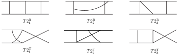
Figure 1: Relevant topologies for the two-loop Weinberg operator

3.1 Two-loop-induced neutrino mass models

In the two-loop case one finds in total 29 topologies out of which only six are relevant, as displayed in fig. 1 [30]. They are relevant in the following sense. The different diagrams one can construct from the full set of topologies can be sorted in three categories:

1. Genuine diagrams: Defined as diagrams for which the absence of one-loop and tree level realizations of $\mathcal{O}_{5}$ is guaranteed. These diagrams are those that one can regard as leading to genuine two-loop models.

2. Non-genuine but finite diagrams: These diagrams involve finite two-loop integrals. They define effective two-loop models: The neutrino mass matrix is one-loop-generated, but one of the “inner” couplings is generated radiatively at the one-loop order.

3. Non-genuine and divergent diagrams: The two-loop integrals for these diagrams are divergent. Thus, all of them are “just” two-loop corrections to either tree or one-loop neutrino mass matrices. From that point of view, therefore, they are of no interest.

Genuine diagrams arise from, and only from, the topologies shown in fig. 1, is in that sense that these topologies are relevant. They however can as well generate non-genuine diagrams falling into categories (II) and (III). Thus, they need to be endowed with further rules (“genuineness rules”) that guarantee genuineness, namely [30]: $(i)$ absence of hypercharge zero fermion $SU(2)$ singlets and triplets or hypercharge two scalar $SU(2)$ triplets; $(ii)$ absence of hypercharge zero scalar EW singlets or triplets; $(iii)$ internal scalars should not have quantum numbers matching those of the standard model Higgs ($H$); $(iv)$ for quartic scalar couplings $H\,H\,S_{1}\,S_{2}$, the following choices: $S_{1,2}=S_{D}$, $S_{1}=S_{S}$ and $S_{2}=S_{T}$, $S_{1}=S_{T}$ and $S_{2}=S_{T}$ (with $S,D,T$ referring to singlet, doublet and triplet), require the difference in hypercharge of these states to be different from $2Y_{H}$ ($Y_{H}$ being the Higgs hypercharge).

Figure 2: The three different classes of genuine two-loop diagrams. The different models arising from these diagrams depend on how the Higgs external legs are attached.

The topologies in fig. 1, combined with the above rules lead to a limited number of genuine diagrams falling in three different non-overlapping classes, as shown in fig. 2. The different genuine two-loop models one can get are determined by the different ways in which the Higgs external legs can be attached to a given diagram. According to the different possibilities, “genuineness rules” allow for a quite limited number of diagrams as follows: 10 diagrams for class (A), 6 diagrams for class (B) and 4 for class (C). Fig. 3 shows the four different diagrams for class (C).

Figure 3: Class (C) possible diagrams.

Once the genuine diagrams are identified, $SU(2)$ quantum numbers of the new fields are fixed by means of direct product decomposition. Due to the two-loop character of the different diagrams, hypercharge is determined up to two arbitrary constants. Sticking to lower EW representations (singlets, doublets and triplets), all possible $SU(2)\times U(1)_{Y}$ quantum numbers have been presented in [30]. These results, along with tabulated two-loop integrals presented as well in [30], provide a complete catalog for radiative neutrino masses at the two-loop order.

4 Conclusions

Among the several mechanism one can envisage for neutrino mass generation, radiatively-induced neutrino masses are a well-motivated option. Certainly, their motivation resides on the fact that in contrast to the “standard” tree level mechanism, loop-induced neutrino masses are (in principle) testable. Here, after sketching the different pathways that can be considered (beyond the tree level and radiative cases), we have discussed the different possibilities for the two-loop case. The results presented here, along with the results from the one-loop systematic classification, complete the model building picture for radiative neutrino masses up to the two-loop order.

References

- [1] S. Weinberg, Phys. Rev. D 22, 1694 (1980).
- [2] F. Bonnet, D. Hernandez, T. Ota and W. Winter, JHEP 0910, 076 (2009) [arXiv:0907.3143 [hep-ph]].
- [3] D. V. Forero, M. Tortola and J. W. F. Valle, Phys. Rev. D 90, no. 9, 093006 (2014) [arXiv:1405.7540 [hep-ph]].
- [4] A. Zee, Phys. Lett. B 93, 389 (1980) [Phys. Lett. B 95, 461 (1980)].
- [5] T. P. Cheng and L. F. Li, Phys. Rev. D 22, 2860 (1980).
- [6] A. Zee, Nucl. Phys. B 264, 99 (1986).
- [7] K. S. Babu, Phys. Lett. B 203, 132 (1988).
- [8] W. Grimus and H. Neufeld, Nucl. Phys. B 325, 18 (1989).
- [9] A. Pilaftsis, Z. Phys. C 55, 275 (1992) [hep-ph/9901206].
- [10] D. Aristizabal Sierra and C. E. Yaguna, JHEP 1108, 013 (2011) [arXiv:1106.3587 [hep-ph]].
- [11] D. Aristizabal Sierra and D. Restrepo, JHEP 0608, 036 (2006) [hep-ph/0604012].
- [12] D. Aristizabal Sierra and M. Hirsch, JHEP 0612, 052 (2006) [hep-ph/0609307].
- [13] D. Aristizabal Sierra, M. Hirsch and S. G. Kovalenko, Phys. Rev. D 77, 055011 (2008) [arXiv:0710.5699 [hep-ph]].
- [14] K. S. Babu and J. Julio, Nucl. Phys. B 841, 130 (2010) [arXiv:1006.1092 [hep-ph]].
- [15] E. Ma, Phys. Rev. D 73, 077301 (2006) [hep-ph/0601225].
- [16] D. Aristizabal Sierra, J. Kubo, D. Restrepo, D. Suematsu and O. Zapata, Phys. Rev. D 79, 013011 (2009) [arXiv:0808.3340 [hep-ph]].
- [17] R. N. Mohapatra and J. W. F. Valle, Phys. Rev. D 34, 1642 (1986).
- [18] E. K. Akhmedov, M. Lindner, E. Schnapka and J. W. F. Valle, Phys. Lett. B 368, 270 (1996) [hep-ph/9507275].
- [19] S. F. King, arXiv:1510.02091 [hep-ph].
- [20] S. Morisi and J. W. F. Valle, Fortsch. Phys. 61, 466 (2013) [arXiv:1206.6678 [hep-ph]].
- [21] D. Aristizabal Sierra, I. de Medeiros Varzielas and E. Houet, Phys. Rev. D 87, no. 9, 093009 (2013) [arXiv:1302.6499 [hep-ph]]; D. Aristizabal Sierra and I. de Medeiros Varzielas, JHEP 1407, 042 (2014) [arXiv:1404.2529 [hep-ph]].
- [22] E. Ma, Phys. Rev. Lett. 81, 1171 (1998) [hep-ph/9805219].
- [23] K. S. Babu and C. N. Leung, Nucl. Phys. B 619, 667 (2001) [hep-ph/0106054].
- [24] K. w. Choi, K. S. Jeong and W. Y. Song, Phys. Rev. D 66, 093007 (2002) [hep-ph/0207180].
- [25] A. de Gouvea and J. Jenkins, Phys. Rev. D 77, 013008 (2008) [arXiv:0708.1344 [hep-ph]].
- [26] F. del Aguila, A. Aparici, S. Bhattacharya, A. Santamaria and J. Wudka, JHEP 1206 (2012) 146 [arXiv:1204.5986 [hep-ph]].
- [27] P. W. Angel, N. L. Rodd and R. R. Volkas, Phys. Rev. D 87, no. 7, 073007 (2013) [arXiv:1212.6111 [hep-ph]].
- [28] Y. Farzan, S. Pascoli and M. A. Schmidt, JHEP 1303, 107 (2013) [arXiv:1208.2732 [hep-ph]].
- [29] F. Bonnet, M. Hirsch, T. Ota and W. Winter, JHEP 1207, 153 (2012) [arXiv:1204.5862 [hep-ph]].
- [30] D. Aristizabal Sierra, A. Degee, L. Dorame and M. Hirsch, JHEP 1503, 040 (2015) [arXiv:1411.7038 [hep-ph]].