March 8, 2024

SURFACE CORRECTIONS TO THE MOMENT OF INERTIA AND SHELL STRUCTURE IN FINITE FERMI SYSTEMS

Abstract

The moment of inertia for nuclear collective rotations is derived within a semiclassical approach based on the Inglis cranking and Strutinsky shell-correction methods, improved by surface corrections within the nonperturbative periodic-orbit theory. For adiabatic (statistical-equilibrium) rotations it was approximated by the generalized rigid-body moment of inertia accounting for the shell corrections of the particle density. An improved phase-space trace formula allows to express the shell components of the moment of inertia more accurately in terms of the free-energy shell correction. Evaluating their ratio within the extended Thomas-Fermi effective-surface approximation, one finds good agreement with the quantum calculations.

PACS numbers: 21.60.Cs, 24.60.Ev

I INTRODUCTION

Many theoretical approaches for nuclear rotations are based on the Inglis cranking model and Strutinsky shell-correction method (SCM) strutMOP , extended to the rotational problems by Pashkevich and Frauendorf pashfrau1975 ; mikhailovepnp . For a deeper understanding of the correspondence between classical and quantum physics of such rotations, it is worth to analyze the shell components of the moment of inertia (MI) within the periodic-orbit theory (POT) gutz ; StrMag1976 ; KMS1979 ; FKMS1998 ; book ; MYAB2011 . In this context, one should refer to Ref. KMS1979 for the semiclassical description of the so called “classical rotation” as an alignment of the particle angular momenta along the symmetry axis. The semiclassical extended-Gutzwiller approach StrMag1976 ; KMS1979 ; MKS1978 also was applied successfully to the description of the magnetic susceptibilities in metallic clusters and quantum dots as a Landau diamagnetic response FKMS1998 (see also Refs. Richter1996 ; MSKB2010 ; belyaev ; GMBBPS2015 ). The perturbation expansion of Creagh book has been used in the POT calculations of the MI shell corrections for the spheroidal-cavity mean field DFP2004 . The semiclassical nature of the cranking model imposes conditions of high angular momenta at larger nuclear deformations. The non-perturbative Gutzwiller POT gutz ; StrMag1976 , extended to the bifurcation phenomena at large deformations MYAB2011 ; MAFM2002 , was applied MSKB2010 to adiabatic (statistical-equilibrium) collective rotations around an axis perpendicular to the symmetry axis in the case of the harmonic-oscillator mean field. The MI for such rotations is described as the sum of the Extended Thomas-Fermi (ETF) MI $\Theta_{\rm ETF}$ bartel ; belyaev and shell corrections $\delta\Theta$ MSKB2010 ; belyaev . By including self-consistency and spin effects into the MI calculations, a more realistic description of collective rotations is obtained within the ETF approach bartel ; ETF_BGH1985 . A phase-space trace formula for the MI shell components $\delta\Theta$ was obtained GMBBPS2015 in terms of the free-energy shell corrections $\delta F$, for integrable highly idealized Hamiltonians such as the deformed harmonic oscillator MSKB2010 and the spheroidal cavity MYAB2011 ; MAFM2002 ; GMBBPS2015 . Spin and pairing effects, as well as higher order $\hbar^{2}$ corrections were however neglected GMBBPS2015 . In the present work, $\hbar^{2}$ surface corrections to the ratio $\delta\Theta/\delta F$ are taken into account within the ETF model in the (leptodermous) effective surface (ES) approach strmagden ; BMRV ; BMR_PS2015 ; BMR_PRC2015 .

II CRANKING MODEL AND SHELL-STRUCTURE

Within the cranking model, the nuclear collective rotation of an independent-particle Fermi system is associated with an eigenvalue problem for the many-body Hamiltonian (Routhian), $\widehat{H}_{\omega}=\widehat{H}\!-\!\omega\widehat{\ell}_{x}$, where $\hat{\ell}_{x}$ is the operator for the particle angular-momentum projection onto the $x$ axis, perpendicular to the symmetry $z$ axis. The frequency $\omega$ and the chemical potential $\lambda$, which are the Lagrange multipliers of the constrained variational problem, are determined by the angular momentum projection $I_{x}$ onto this $x$ axis and the particle number conservation $N$. The MI $\Theta_{x}$ can be considered as a susceptibility (Refs. FKMS1998 ; Richter1996 ; MSKB2010 ; belyaev ; GMBBPS2015 ):

$$\Theta_{x}=\partial\langle\hat{\ell}_{x}\rangle_{\omega}/\partial\omega=\partial^{2}E(\omega)/\partial\omega^{2}\;,$$ (1)

where $E(\omega)$ is the quantum average of the Hamiltonian $\widehat{H}$, i.e. the energy of the yrast line $E(I_{x},N)$ resulting from these two constraints. Using the coordinate representation for the MI $\Theta_{x}$ in terms of the one-body semiclassical Gutzwiller expansion for the Green’s function, for the adiabatic statistically equilibrium rotations in the nearly local approximation one obtains the MI phase-space trace formula GMBBPS2015 :

$$\Theta_{\rm scl}\approx d_{s}\,m\int{\rm d}\varepsilon\;\varepsilon\;n(\varepsilon)\int\frac{{\rm d}{\bf r}{\rm d}{\bf p}}{(2\pi\hbar)^{3}}\frac{r_{\perp}^{2}}{\varepsilon}$$ (2)

$$\times g_{\rm scl}({\bf r},{\bf p};\varepsilon)=\Theta_{\rm ETF}+\delta\Theta_{\rm scl}\;,$$

where $m$ is the nucleon mass, $n(\varepsilon)$ the occupation number, $d_{s}$ the spin (spin-isospin) degeneracy, and $r_{\perp}^{2}\!=\!y^{2}+z^{2}$ in Cartesian coordinates. Starting from the Wigner distribution function $f({\bf r},{\bf p})$, one defines the one-body density $g({\bf r},{\bf p};\varepsilon)$ in the phase space ${\bf r},{\bf p}$ and energy $\varepsilon$ as the derivative of $f({\bf r},{\bf p})$ with respect to $\varepsilon$ [see Eq. (A12)]. This density $g$ can be written, like traditionally done, as MSKB2010 ; GMBBPS2015 ; belyaev

$$g_{\rm scl}({\bf r},{\bf p};\varepsilon)=g_{\rm ETF}({\bf r},{\bf p};\varepsilon)+\delta g({\bf r},{\bf p};\varepsilon)\;,$$ (3)

where $g_{\rm ETF}({\bf r},{\bf p};\varepsilon)$ is the ETF component and $\delta g({\bf r},{\bf p};\varepsilon)$ the shell correction (see Ref. GMBBPS2015 for the relation of $g_{\rm scl}({\bf r},{\bf p};\varepsilon)$ to the Gutzwiller Green’s function expansion over classical trajectories).

In what follows we shall take advantage of the strong resemblance of the MI (2) with the semiclassical single-particle energy. The only difference is that an additional factor $\leavevmode\nobreak\ mr_{\perp}^{2}/\varepsilon\leavevmode\nobreak\$ appears in Eq. (2). The same subdivision in terms of the ETF and shell components is obtained at finite temperatures $T$ after a statistical averaging in Eq. (2) where

$$\delta\Theta_{\rm scl}\approx m\,\langle r_{\perp}^{2}/\varepsilon\rangle\;\delta F_{\rm scl}\;,$$

$$\delta F_{\rm scl}={\mbox{\rm Re}}\sum_{\rm PO}\frac{\pi t_{\rm PO}T/\hbar}{\hbox{sinh}(\pi t_{\rm PO}T/\hbar)}\;\delta E_{\rm PO}\;.$$ (4)

Brackets $\langle\cdots\rangle$ indicate an average over the variables ${\bf r}$, ${\bf p}$, and $\varepsilon$ with a weight $\varepsilon$, i.e.,

$$\langle\,\frac{r_{\perp}^{2}}{\varepsilon}\,\rangle=\frac{\int{\rm d}\varepsilon\;\varepsilon\;n(\varepsilon)\int{\rm d}{\bf r}\,{\rm d}{\bf p}\;\frac{r_{\perp}^{2}}{\varepsilon}g_{\rm scl}({\bf r},{\bf p};\varepsilon)}{\int{\rm d}\varepsilon\;\varepsilon\;n(\varepsilon)\int{\rm d}{\bf r}\,{\rm d}{\bf p}\;g_{\rm scl}({\bf r},{\bf p};\varepsilon)}\;\;.$$ (5)

In Eq. (II), $\delta F_{\rm scl}$ is the semiclassical free-energy shell correction and $\delta E_{\rm PO}$ the periodic-orbit (PO) component of the energy shell correction,

$$\delta E\approx\delta E_{\rm scl}={\mbox{\rm Re}}\sum_{\rm PO}\delta E_{\rm PO}\quad\mbox{with}\quad$$

$$\delta E_{\rm PO}\propto\frac{\hbar^{2}}{t_{\rm PO}^{2}}\;\hbox{exp}\left[\frac{i}{\hbar}\;S_{\rm PO}(\lambda)-\frac{i\pi}{2}\;\mu_{\rm PO}\right]\;.$$ (6)

The period $\leavevmode\nobreak\ t_{\rm PO}\leavevmode\nobreak\$, and the action $\leavevmode\nobreak\ S_{\rm PO}(\varepsilon)\leavevmode\nobreak\$ for the particle motion along the PO are taken at the chemical potential $\varepsilon\!=\!\lambda\!\approx\!\varepsilon_{F}$ (at $\omega\!=\!0$ and $T\!=\!0$) where $\varepsilon_{F}$ is the Fermi energy book ; MYAB2011 ; belyaev . The Maslov phase $\mu_{\rm PO}$ is determined by the number of the caustic and turning points along the PO. POs appear by the improved stationary phase method (ISPM) through integrations over the phase space variables MYAB2011 ; MAFM2002 ; belyaev ; GMBBPS2015 . For the phase-space average $\langle r_{\perp}^{2}/\varepsilon\rangle$ in Eq. (5) one again obtains approximately a decomposition into ETF and shell-correction contributions through the distribution function $g_{\rm scl}({\bf r},{\bf p};\varepsilon)$.

III SURFACE CORRECTIONS

Using the inverse Laplace transformation (A12) one arrives at an expansion up to order $\hbar^{2}$ of the smooth semiclassical one-body distribution function (Appendix A),

$$g_{\rm ETF}({\bf r},{\bf p};\varepsilon)\approx g_{\rm TF}({\bf r},{\bf p};\varepsilon)+g_{\rm S}({\bf r},{\bf p};\varepsilon)\;,$$ (7)

with the TF and surface components,

$$g_{\rm TF}({\bf r},{\bf p};\varepsilon)=\delta\left(\varepsilon-H_{\rm cl}({\bf r},{\bf p})\right)\;,$$ (8)

$$g_{\rm S}({\bf r},{\bf p};\varepsilon)=\hbar^{2}\left\{-\frac{\nabla^{2}V}{4m}\;\frac{\partial^{2}\delta\left(\varepsilon-H_{\rm cl}({\bf r},{\bf p})\right)}{\partial\varepsilon^{2}}\right.$$ (9)

$$+ \left.\left[\frac{\left(\nabla V\right)^{2}}{6m}+\frac{\left({\bf p}\nabla\right)^{2}V}{6m^{2}}\right]\;\frac{\partial^{3}\delta\left(\varepsilon-H_{\rm cl}({\bf r},{\bf p})\right)}{\partial\varepsilon^{3}}\right.$$

$$- \left.\frac{\left({\bf p}\nabla V\right)^{2}}{8m^{2}}\;\frac{\partial^{4}\delta\left(\varepsilon-H_{\rm cl}({\bf r},{\bf p})\right)}{\partial\varepsilon^{4}}\right\}\;.$$

Here $H_{\rm cl}({\bf r},{\bf p})\!=\!p^{2}/(2m)\!+\!V({\bf r})$ is the classical Hamiltonian with the mean-field potential $V({\bf r})$ . Gradients of the potential V in the surface correction $g_{\rm S}$ of order $\hbar^{2}$ can be expressed, within the ETF method ETF_BGH1985 ; book , to the same $\hbar^{2}$ order, in terms of gradients of the TF particle density [see Eqs. (A10) and (A11)],

$$\rho_{\rm TF}=d_{s}[2m(\lambda-V({\bf r}))]^{3/2}/(6\pi^{2}\hbar^{3})\;.$$ (10)

From Eqs.  (3), (7)–(9) and (5) one obtains, for the spheroidal cavity, within the ETF ES approximation up to $\hbar^{2}$ corrections,

$$\langle r_{\perp}^{2}/\varepsilon\rangle_{\rm ETF}\approx\frac{a^{2}+b^{2}}{3\lambda}\;\frac{1+\Theta_{\rm S}/\Theta_{\rm TF}}{1+E_{\rm S}/E_{\rm TF}}\;,$$ (11)

where $a$ and $b$ are the semi-axes of the spheroid. Imposing volume conservation requires that $a^{2}b=R^{3}$, where $R$ is the radius of the equivalent sphere. $E_{\rm TF}$, $\Theta_{\rm TF}$ and $E_{\rm S}$, $\Theta_{\rm S}$ are the TF and $\hbar^{2}$ ETF surface components, respectively book . The surface energy $\leavevmode\nobreak\ E_{\rm S}\!=\!\sigma\mathcal{S}\!=\!b_{\rm S}N^{2/3}\leavevmode\nobreak\$ with the spheroid area $\mathcal{S}$ and surface energy constant $b_{\rm S}=4\pi r_{0}^{2}\sigma$ is determined by the surface tension $\sigma$ of the capillary pressure. Within the ETF model, $\sigma$ is defined by the $\hbar^{2}$ correction to the kinetic energy (Appendix B),

$$\sigma=\frac{\hbar^{2}}{72m}\;\int_{-\infty}^{\infty}\frac{\hbox{d}\xi}{\rho_{\rm TF}}\;\left(\frac{\partial\rho_{\rm TF}}{\partial\xi}\right)^{2}\;,$$ (12)

where $\xi$ is locally the distance from a given point ${\bf r}$ to the ES book ; belyaev ; strmagden . The surface corrections in Eq. (11) are given by

$${}\frac{E_{\rm S}}{E_{\rm TF}} = \frac{5b_{\rm S}\mathcal{S}}{12\pi\eta^{2/3}a^{2}\lambda\;N^{1/3}}\qquad\mbox{and}$$

$$\frac{\Theta_{\rm S}}{\Theta_{\rm TF}} = 5b_{\rm S}\;\frac{\eta^{2}I_{0}+\pi(1-2\eta^{2})I_{1}}{\pi^{2}\eta^{2/3}(1+\eta^{2})\lambda\;N^{1/3}}\;,$$ (13)

where

$$I_{0}=1+\frac{\eta^{2}\arctan\sqrt{\eta^{2}-1}}{\sqrt{\eta^{2}-1}}$$

and

$$I_{1} = \frac{2\eta}{3\sqrt{\eta^{2}-1}}\left[(2\eta^{2}-1)E\left(\sqrt{\eta^{2}-1}/\eta\right)\right.$$ (14)

$$- \left.K\left(\sqrt{\eta^{2}-1}/\eta\right)\right]$$

with $E(\kappa)$ and $K(\kappa)$ being the complete elliptic integrals byrd . The deformation parameter is given by $\eta=b/a$. In units of the classical rigid-body (TF) MI, $\Theta_{\rm TF}\!=\!m\left(a^{2}+b^{2}\right)N/5$, one finally obtains

$$\frac{\delta\Theta_{x}}{\Theta_{\rm TF}}=\frac{5\left(1+\Theta_{\rm S}/\Theta_{\rm TF}\right)}{1+E_{\rm S}/E_{\rm TF}}\frac{\delta F}{3N\lambda}\;.$$ (15)

IV DISCUSSION OF RESULTS

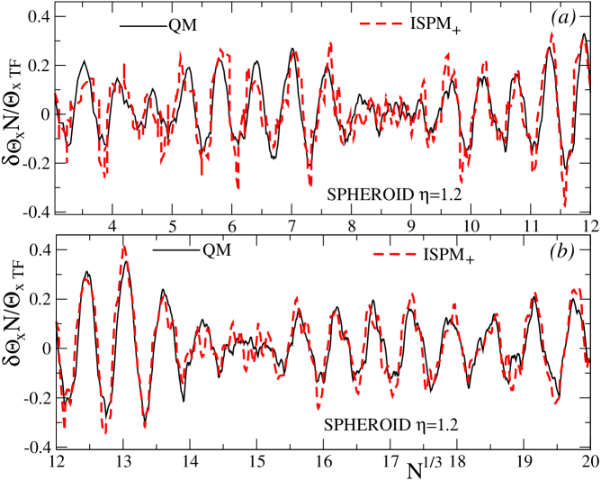
Figure 1: (Color online) MI shell components $\delta\Theta_{x}$ (in TF units) as function of $N^{1/3}$ at deformation $\eta=b/a=1.2$ obtained in a quantum-mechanical (QM) and a semiclassical calculation, including surface corrections (ISPM₊) for smaller (upper part (a)) and larger (lower part (b)) particle numbers.

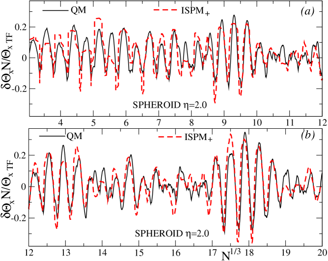
Figure 2: (Color online) Same as Fig. 1 but for a deformation of $\eta=2.0$.

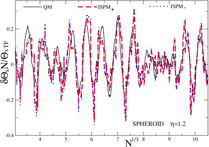
Figure 3: (Color online) Comparison between the MI shell components $\delta\Theta_{x}$ (in TF units) obtained with (ISPM₊) and without (ISPM_-) surface corrections as function of $N^{1/3}$. For comparison the quantum result (black solid line) is also shown. The deformation is $\eta=1.2$.

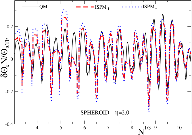
Figure 4: (Color online) Same as Fig. 3 but for $\eta=2.0$.

Figures 1 and 2 show a comparison between the semiclassical ISPM MI shell corrections (II) obtained with (index $+$) surface terms and the quantum-mechanical (QM) result. The latter is determined through the ETF average (11) for $\langle r_{\perp}^{2}/\varepsilon\rangle$ with a realistic surface energy constant $b_{\rm S}\approx 20$ MeV whereas the energy shell correction $\delta E$ (equal $\delta F$ at zero temperature $T$) is calculated by the SCM using the quantum spectrum. A large supershell effect appears in $\delta\Theta_{x}$, especially for larger deformations in the PO bifurcation region (Figs. 2 and 4). The effect of the surface correction, Eq. (III), is analyzed in Figs. 3 and 4 that show, together with the result of the quantum calculation, the shell components $\delta\Theta_{x}/\Theta_{\rm TF}$ obtained with (ISPM₊) and without (ISPM_-) these surface corrections. The difference between both curves is seen to be more important for small particle numbers, which can be easily understood since the surface corrections decreases as $N^{-1/3}$ as seen from Eq. (III). The contribution of the shorter three-dimensional orbits bifurcated from the equatorial ones are dominating in the case of large deformations (Fig. 2), in contrast to the small deformation region where the meridian orbits are predominant (Figs. 1 and 3), in accordance with Refs. MYAB2011 ; MAFM2002 . One also observes that the surface corrections become more significant with increasing deformation of the system.

For small temperatures one has $\delta F_{\rm scl}\!\approx\!\delta E_{\rm scl}$, and therefore, a remarkable interference of the dominant short three-dimensional and meridian orbits is shown in Refs. MYAB2011 ; MAFM2002 ; GMBBPS2015 . Their bifurcations in the superdeformed region give essential contributions to the MI through the (free) energy shell corrections. With increasing temperature the shorter equatorial orbits become dominating, as seen analytically from the exponentially decreasing temperature-dependent factor in Eq. (II).

The shell corrections (II) to the MI are relatively much smaller than the classical rigid-body (TF) component. This is similar to the (free) energy shell corrections $\delta E$ (or $\delta F$) as compared with the ETF volume and surface energy. However, many important physical effects, such as fission isomerism and high spin physics depends basically on the shell effects. Our non-perturbation results for the MI shell corrections can be applied for larger rotational frequencies and larger deformations $\eta\!\sim\!1.5\!-\!2.0$ where the bifurcations play the dominating role.

V SUMMARY AND CONCLUSIONS

Within the non-perturbative Gutzwiller POT we derived the MI shell component $\delta\Theta$ in terms of the free-energy shell correction $\delta F$ for any mean-field potential by taking into account the ETF $\hbar^{2}$ corrections in the effective surface approximation. For the deformed spheroidal cavity, we found a good agreement between the semiclassical POT and quantum results for $\delta\Theta$ at several deformations and temperatures. The surface corrections become more significant with increasing deformations and decreasing particle numbers. With increasing temperature, one finds the generally observed exponential decrease of the shell effects. For large deformations and small temperatures, one observes some remarkable supershell effects due to the interference of three-dimensional and meridian orbits bifurcating from the equatorial orbits.

For future research in this field, it would be valuable to include the neutron-proton asymmetry BMRV ; BMR_PS2015 ; BMR_PRC2015 and the spin degrees of freedom into the semiclassical MI shell calculations belyaev . The latter lead to the well-known spin-orbit splitting which significantly changes the nuclear shell structure and accounts for spin paramagnetic effects belyaev . The MI expressions obtained analytically at the present stage have therefore only a somewhat restricted values for the use in real nuclei, but could be directly applied to the magnetic susceptibility for metallic clusters and quantum dots FKMS1998 . The extension of the POT to the MI shell correction calculations with the inclusion of the spin degree of freedom would constitute an essential progress in understanding the relation between the nuclear MI and the free-energy shell corrections. For a more realistic study, let us also mention the inclusion of pairing correlations, especially far from deformed magic nuclei and non-adiabatic effects. The work along these lines is in progress.

ACKNOWLEDGMENTS

We would like to thank K. Arita, M. Brack, M. Matsuo, K. Matsuyanagi, and K. Pomorski for helpful and stimulating discussions. One of us (A.G.M.) is also very grateful for nice hospitality and financial support during his working visits of the National Centre for Nuclear Research (Poland), the Strasbourg Institut Pluridisplinaire Hubert Curien (France), the Nagoya Institute of Technology (Japan), and Japanese Society of Promotion of Sciences, Grant No. S-14130.

Appendix A: THE WIGNER-KIRKWOOD METHOD

The Wigner-Kirkwood method starts with the Gibbs operator book , $\hat{C}_{\beta}\!=\!\hbox{exp}(-\beta\hat{H})$, where $\hat{H}$ is the quantum-mechanical Hamiltonian. In the case that $\hat{H}$ is time independent, the coordinate-space representation of the Gibbs operator, the so-called Bloch density matrix, is given by

$$C({\bf r}_{1},{\bf r}_{2};\beta)=\sum_{i}\psi^{\ast}_{i}({\bf r}_{1})\;\hbox{exp}(-\beta\;\varepsilon_{i})\;\psi_{i}({\bf r}_{2}),$$ (A1)

where $\psi_{i}$ and $\varepsilon_{i}$ are the eigenfunctions and eigenvalues of the Hamiltonian ($\hat{H}\psi_{i}\!=\!\varepsilon_{i}\psi_{i}$). Therefore, after formally replacing $\beta\!=\!it/\hbar$, the Bloch density matrix $C({\bf r}_{1},{\bf r}_{2};\beta)$ is seen to be nothing but the one-body time-dependent propagator (Green’s function) $K({\bf r}_{1},{\bf r}_{2};t)$ and one can use the corresponding Schrödinger equation for the calculation of $C({\bf r}_{1},{\bf r}_{2};\beta)$ book . Note that the POT in the extended Gutzwiller version starts with the solution of this equation for the propagator $K({\bf r}_{1},{\bf r}_{2};t)$ in terms of the Feynman path integral. Its calculation by the stationary phase method leads to the semiclassical expression for $K({\bf r}_{1},{\bf r}_{2};t)$, and then, one can get the semiclassical expansion of the Green’s function, $G({\bf r}_{1},{\bf r}_{2};\varepsilon)$, and its traces, namely the level density, $g(\varepsilon)$, and the particle density $\rho({\bf r})$ (at ${\bf r}_{1}\!\rightarrow\!{\bf r}_{2}\!=\!{\bf r}$). The shell components of these densities can be expressed in terms of the closed trajectories (see the main text for the case of the oscillating level-density part written in terms of POs). Thus, the POT can be developed for the Bloch density matrix $C({\bf r}_{1},{\bf r}_{2};\beta)$ itself.

In order to solve semiclassically the Schrödinger equation for the Bloch function $C({\bf r}_{1},{\bf r}_{2};\beta)$, one can make a transformation, first from ${\bf r}_{1}$ and ${\bf r}_{2}$ to the center-of-mass and relative coordinates, ${\bf r}\!=\!({\bf r}_{1}\!+\!{\bf r}_{2})/2$ and ${\bf s}\!=\!{\bf r}_{2}\!-\!{\bf r}_{1}$, and then, by the Fourier transformation to the phase-space variables, $\{{\bf r},{\bf p}\}$, what corresponds to a Wigner transformation from $C({\bf r}_{1},{\bf r}_{2};\beta)$ to $C_{W}({\bf r},{\bf p};\beta)$,

$$C_{W}({\bf r},{\bf p};\beta) = \int\frac{\hbox{d}{\bf s}}{(2\pi\hbar)^{3}}\;C({\bf r}-{\bf s}/2,{\bf r}+{\bf s}/2;\beta)$$ (A2)

$$\times \hbox{exp}\left(i{\bf p}{\bf s}/\hbar\right)\;.$$

This reduces one complicated Schrödinger equation to an infinite system of much simpler first-order ordinary differential equations (at each power of $\hbar$, see Ref. book ) which can be analytically integrated.

The advantage of the Wigner-Kirkwood method is obviously to generate smooth quantities averaged over many quantum states to smooth out quantum oscillations like shell effects. The POT on the contrary is aimed at the derivation of analytical expressions for the shell components of the partition function, and thereby of the level and particle densities. In the Wigner-Kirkwood method, the main term of the expansion of $C_{W}({\bf r},{\bf p};\beta)$ is proportional to the classical distribution function $f_{\rm cl}({\bf r},{\bf p})$, and $\hbar$ corrections can be obtained by solving a simple system of differential equations at each power of $\hbar$. Strictly speaking there is no convergence of this asymptotical expansion because of presence of the $\hbar$ in the rapidly oscillating exponents. Therefore, to get the convergent series in $\hbar$ of the ETF approach, one first has to use local averaging in the phase space variables and then, expand smooth quantities in a $\hbar$ series, in contrast to the shell-structure POT. In this way, the simple ETF $\hbar$ expansions of local quantities such as the particle density $\rho({\bf r})$, kinetic energy density $\tau({\bf r})$, and level density $g(\varepsilon)$ are obtained.

The canonic partition function $\mathcal{Z}(\beta)$ is obtained by integrating over the whole space the diagonal Bloch matrix $C({\bf r},{\bf r};\beta)\!=\!C({\bf r};\beta)$,

$$\mathcal{Z}(\beta)=\int\hbox{d}{\bf r}\;C({\bf r};\beta)=\sum_{i}\hbox{exp}(-\beta\varepsilon_{i})\;.$$ (A3)

The trace, $\mathcal{Z}\!=\!\mbox{Tr}\{\hbox{exp}(-\beta\hat{H})\}$, can be taken for any complete set of states. For the semiclassical expansion involving an integral over the phase space, it is more convenient to take plane waves as the complete set. We may then write

$$\mathcal{Z}(\beta)=\int\frac{\hbox{d}{\bf r}\;\hbox{d}{\bf p}}{(2\pi\hbar)^{3}}e^{-i{\bf p}{\bf r}/\hbar}\;e^{-\beta\hat{H}}\;e^{i{\bf p}{\bf r}/\hbar}\;.$$ (A4)

As the kinetic operator in $\hat{H}$ does not commute with the potential $V({\bf r})$, it is convenient to use the following representation book :

$$e^{-\beta\hat{H}}e^{i{\bf p}{\bf r}/\hbar}=e^{-\beta H_{\rm cl}}\;e^{i{\bf p}{\bf r}/\hbar}\;w({\bf r},{\bf p};\beta)\;,$$ (A5)

where $H_{\rm cl}$ is the classical Hamiltonian that appears in Eqs. (8) and (9). Solving the Schrödinger equation for the function $w$ with the boundary condition $\mbox{lim}_{\beta\to 0}w({\bf r},{\bf p};\beta)\!=\!1$, one assumes that $w({\bf r},{\bf p};\beta)$ can be expanded in a power series in $\hbar$:

$$w=1+\hbar w_{1}+\hbar^{2}w_{2}+\cdots\;.$$ (A6)

Equating terms of the same power in $\hbar$ from both sides of this differential equation, one obtains the $\hbar$ corrections:

$$w_{1}=-\frac{i\beta^{2}}{2m}\;{\bf p}\cdot\nabla V,\hskip 51.21504pt$$ (A7)

and

$$w_{2}=-\frac{\beta^{2}}{4m}\nabla^{2}V+\frac{\beta^{3}}{6m}\left(\nabla V\right)^{2}$$ (A8)

$$- \frac{\beta^{4}}{8m^{2}}\left({\bf p}\cdot\nabla V\right)^{2}+\frac{\beta^{3}}{6m^{2}}\left({\bf p}\cdot\nabla\right)^{2}V\;.$$

The semiclassical series for the partition function takes then the form:

$$\mathcal{Z}(\beta) = \int\frac{\hbox{d}{\bf r}\;\hbox{d}{\bf p}}{(2\pi\hbar)^{3}}e^{-i{\bf p}{\bf r}/\hbar}\;e^{-\beta H_{\rm cl}}$$ (A9)

$$\times \left(1+\hbar w_{1}+\hbar^{2}w_{2}+...\right)\;.$$

Differentiating the TF particle density $\rho_{\rm TF}$ (10) and solving the obtained linear system of equations for the gradients of the potential, one finds

$$\left(\nabla V\right)^{2}=\left(\frac{\pi^{2}\hbar^{2}}{m(3\pi^{2}\rho)^{1/3}}\right)^{2}\left(\nabla\rho\right)^{2},$$ (A10)

$$\nabla^{2}V=\frac{\pi^{2}\hbar^{2}}{m(3\pi^{2}\rho)^{1/3}}\left[\frac{\left(\nabla\rho\right)^{2}}{3\rho}-\nabla^{2}\rho\right]$$ (A11)

where the subscript TF on the density has been omitted. These expressions are more convenient to use in the more general case, including billiard systems, in particular, the spheroidal cavity.

For calculations of the semiclassical distribution function $g({\bf r},{\bf p};\varepsilon)$, one can apply the inverse Laplace transformation:

$$g({\bf r},{\bf p};\varepsilon)=\frac{\partial f({\bf r},{\bf p})}{\partial\varepsilon}=\frac{1}{2\pi i}\;\int_{\beta_{r}-i\infty}^{\beta_{r}+i\infty}d\beta\;$$ (A12)

$$\times \hbox{exp}\left[\beta\left(\varepsilon-H_{\rm cl}\right)\right]\left(1+\hbar w_{1}+\hbar^{2}w_{2}\right),$$

where $w_{1}$ and $w_{2}$ are the semiclassical corrections of Eqs. (A7) and (A8). The integration in the complex $\beta$ plane in Eq. (A12) has to be taken along the imaginary axis, at a distance $\beta_{r}$ such that all singularities are located at its left. The linear term in $\hbar$, i.e. the term $w_{1}$ that is linear in ${\bf p}$, does not contribute to the phase-space (momentum) integral for the energy $E$ and for the MI $\Theta$ in Eq. (2). Calculating the integral in Eq. (A12) using Eq. (A8), one arrives, after some simple algebraic transformations, at Eq. (9).

Appendix B: THE ES METHOD

For independent nucleons bound in a potential well, the energy density $\mathcal{E}(\rho)$ of symmetric nuclear matter ($N\!=\!Z\!=\!A/2$) is found to be strmagden ; BMRV ; BMR_PS2015 ; BMR_PRC2015

$$\mathcal{E}\left(\rho\right)=-b_{\rm V}\rho+\rho\varepsilon(\rho)+\Gamma\;\left(\nabla\rho\right)^{2}/(4\rho)\;,$$ (B1)

where $b_{V}$ is the separation energy per particle, $\varepsilon(\rho)\!\approx\![K/18\rho^{2}_{\infty}]\left(\rho\!-\!\rho_{\infty}\right)^{2}$, and where $K$ and $\rho_{\infty}$ are the incompressibility modulus and the particle density of infinite nuclear matter, and $\Gamma\!=\!\hbar^{2}/(18m)$. For simplicity we neglect spin-orbit and asymmetry terms. A variation of the energy functional, $E\!=\!\int\hbox{d}{\bf r}\;\mathcal{E}[\rho({\bf r})]$ with the energy density (B1) leads to the Lagrange equation strmagden :

$$\frac{\Gamma}{2\rho}\;\triangle\rho-\frac{\Gamma}{4\rho^{2}}\left(\nabla\rho\right)^{2}-\frac{\hbox{d}}{\hbox{d}\rho}\left[\rho\;\varepsilon(\rho)\right]+\Lambda=0\;,$$ (B2)

where $\Lambda=\lambda\!+\!b_{\rm V}$ is the correction to the separation energy $-b_{\rm V}$ in the chemical potential $\lambda$. This correction is proportional to a small leptodermous parameter $a/R\!\sim\!A^{-1/3}$ for heavy nuclei. Introducing a local orthogonal-coordinate system with a coordinate $\xi$ that defines the distance from a given point ${\bf r}$ to the effective surface (ES), one gets for the particle density $\rho_{0}$, in leading order in the leptodermous parameter $a/R$, a simple ordinary differential equation

$$\hbox{d}\rho_{0}/\hbox{d}\xi=-2\rho_{0}\;\varepsilon^{1/2}(\rho_{0})/\Gamma^{1/2}\;.$$ (B3)

This equation can be solved analytically for the quadratic approximation to $\varepsilon(\rho)$. Transforming the differential equation (B3) to one for the dimensionless particle density,

$$w(x) = \rho(\xi)/\rho_{\infty}\quad\mbox{with}\quad x=\xi/a\;,$$

$$\epsilon(w) = (18/K)\;\varepsilon(\rho)=(1-w)^{2}\;,$$ (B4)

one finds

$$w^{\prime}(x)=-\zeta w\sqrt{\epsilon(w)}\;,$$ (B5)

where $\zeta\!=\!2a\sqrt{K/(18\Gamma)}$. Differentiating once more and using the fact that, by definition, $w^{\prime\prime}(x)\!=\!0$ at the ES, one gets the boundary condition for $w_{0}\!=\!w(x=0)$:

$$2\epsilon(w_{0})+w_{0}\epsilon^{\prime}(w_{0})=0\;.$$ (B6)

With Eq. (V) for $\epsilon(w)$, one finds the solution $w_{0}\!=\!1/2$. Integrating Eq. (B5) using the boundary condition (B6), one obtains the explicit solution

$$w(x)=\left[1+\hbox{exp}\left(\zeta x\right)\right]^{-1}\;,$$ (B7)

which tends asymptotically (for $x\!\rightarrow\!\infty$) to $w(x)\!\rightarrow\!\hbox{exp}(-\zeta x)$. Therefore, one can define the diffuseness parameter $a$ from the usual condition, $\zeta\!=\!1$ so that the particle density $w(x)$ will be decreasing at large $x$ as $\hbox{exp}(-x)$:

$$a=\sqrt{9\Gamma/(2K)}=\sqrt{\hbar^{2}/(4mK)}\;.$$ (B8)

Another limiting case of finite constants of the potential part of the energy density [in front of $(\nabla\rho)^{2}$], including the spin-orbit and asymmetry terms but neglecting the kinetic energy term proportional to $\Gamma$ in Eq. (B1), was investigated in Refs. BMRV ; BMR_PS2015 ; BMR_PRC2015 .

For the energy $E$ with Eq. (B1), one has

$$E = -b_{\rm V}A+\int\hbox{d}{\bf r}\left[\frac{\Gamma}{4}\,\frac{\left(\nabla\rho\right)^{2}}{\rho}+\rho\varepsilon(\rho)\right]$$ (B9)

$$= E_{\rm V}+E_{\rm S}\;,$$

where $E_{\rm V}\!=\!-b_{\rm V}A$ is the volume and $E_{\rm S}\!=\!\sigma S$ the surface component with the surface-tension coefficient

$$\sigma=\frac{\Gamma}{2}\int_{-\infty}^{\infty}\frac{\hbox{d}\xi}{\rho_{0}}\;\left(\frac{\partial\rho_{0}}{\partial\xi}\right)^{2}\;.$$ (B10)

For the calculation of the surface energy $E_{\rm S}$ from Eq. (B9), one needs the particle density $\rho\!\approx\!\rho_{0}$ at leading order in the leptodermous parameter $a/R$. Due to the spatial derivatives in its integrand, and the definition of $\epsilon(w)$ [Eq. (V)], this surface integration gives, in addition to the integrand, the contribution of order $a/R$. Therefore, according to the Lagrange equation at this order, Eq. (B3), the two terms in square brackets in the integral in Eq. (B9) turn out to be identical. Thus, we arrived at Eq. (B10). Using Eqs. (B3) and (B10) for the surface-tension coefficient, one finds (after transforming to dimensionless quantities and changing the integration variable from $x$ to $w$) the analytical result

$$\sigma=(\hbar\rho_{\infty}/36)\;\sqrt{K/m}\;.$$ (B11)

Other limit cases are considered in Refs. BMRV ; BMR_PS2015 ; BMR_PRC2015 .

References

- (1) V.M. Strutinsky Nucl. Phys. A 95 420 (1967); 1 (1968).
- (2) V.V. Pashkevich and S. Frauendorf, Sov. J. Nucl. Phys. 20, 588 (1975).
- (3) I.N. Mikhailov, K. Neergard, V.V. Pashkevich, and S. Frauendorf, Sov. J. Part. Nucl. 8 550 (1977).
- (4) M. Gutzwiller, J. Math. Phys. 12, 343 (1971); M. Gutzwiller, Chaos in Classical and Quantum Mechanics (Springer-Verlag, New York, 1990).
- (5) V.M. Strutinsky, Nucleonika 20, 679 (1975); V.M. Strutinsky and A.G. Magner, Sov. J. Part. Nucl. 7, 138 (1976).
- (6) V.M. Kolomietz, A.G. Magner, and V.M. Strutinsky, Sov. J. Nucl. Phys. 29 758 (1979).
- (7) S. Frauendorf, V.M. Kolomietz, A.G. Magner, and A.I. Sanzhur, Phys. Rev. B 58 5622 (1998).
- (8) M. Brack and R.K. Bhaduri, Semiclassical Physics. Frontiers in Physics, No 96, 2nd ed. (Westview Press, Boulder, CO, 2003).
- (9) A.G. Magner, Y.S. Yatsyshyn, K. Arita, and M. Brack, Phys. At. Nucl. 74 1445 (2011).
- (10) A.G. Magner, V.M. Kolomietz, V.M. Strutinsky, Sov. J. Nucl. 28, 764 (1978).
- (11) K. Richter, D. Ulmo, and R.A. Jalabert, Phys. Rep. 276, 1 (1996).
- (12) A.G. Magner, A.S. Sitdikov, A.A. Khamzin, and J. Bartel, Phys. Rev. C 81 064302 (2010).
- (13) D.V. Gorpinchenko, A.G. Magner, J. Bartel, and J.P. Blocki, Phys. Scr., T 90, 114008 (2015).
- (14) A.G. Magner, D.V. Gorpinchenko, and J. Bartel, Phys. At. Nucl. 77 1229 (2014).
- (15) M.A. Deleplanque, S. Frauendorf, V.V. Pashkevich et al. Phys. Rev. C69 044309 (2004).
- (16) A.G. Magner, K. Arita, S.N. Fedotkin, and K. Matsuyanagi, Prog. Theor. Phys. 108 853 (2002).
- (17) K. Bencheikh, P. Quentin, and J. Bartel, Nucl. Phys. A 571, 518 (1994).
- (18) M. Brack, C. Guet, and H.-B. Håkansson, Phys. Rep. 123, 275 (1985).
- (19) V.M. Strutinsky, A.G. Magner, and V.Yu. Denisov, Z. Phys. A 322, 149 (1985).
- (20) J.P. Blocki, A.G. Magner, P. Ring, and A.A. Vlasenko, Phys. Rev. C 87, 044304 (2013).
- (21) J.P. Blocki, A.G. Magner, and P. Ring, Phys. Scr. T 90, 114009 (2015).
- (22) J.P. Blocki, A.G. Magner, and P. Ring, Phys. Rev. C92, 064311 (2015).
- (23) P.F. Byrd and M.D. Friedman, Handbook of Elliptic Integrals for Engineers and Scientists (Springer-Verlag, New York, 1971).