Design of metallic nanoparticles gratings for filtering properties in the visible spectrum

Abstract

Plasmonic resonances in metallic nanoparticles are exploited to create efficient optical filtering functions. A Finite Element Method is used to model metallic nanoparticles gratings. The accuracy of this method is shown by comparing numerical results with measurements on a two-dimensional grating of gold nanocylinders with elliptic cross section. Then a parametric analysis is performed in order to design efficient filters with polarization dependent properties together with high transparency over the visible range. The behavior of nanoparticle gratings is also modelled using the Maxwell-Garnett homogenization theory and analyzed by comparison with the diffraction by a single nanoparticle. The proposed structures are intended to be included in optical systems which could find innovative applications.

I Introduction

Metallic nanoparticles supporting plasmonic resonances can be used to design optical functions, for instance filtering properties, or chemical and bio-sensing Perney06 ; Yih06 . Such systems offer several advantages, like the possibility to control the operating wavelength with the nature of the metal, the size of the particles, the polarization of the illumination… In this paper we focus on the design of spectral filtering property in reflectivity, i.e. frequency selective mirror property. In particular, challenges lie in obtaining a narrow reflexion peak while keeping absorption losses as low as possible together with a transmission level averaged over the visible range as high as possible.

Reflective color filters based on plasmonic resonators have already been proposed in the literature. In kumar2012printing , different arrays of metallic nanodisks are deposited on a back reflector made of silver and gold to print a color image at the optical diffraction limit. Dense silver nanorods arrays are used in junahuang2013reflective to create reflective color filters at specific wavelengths depending on the arrays geometry. Nevertheless, in these propositions, the overall transmission remains low. Core-shell nanoparticles, made of silica and silver and embedded into a polymer matrix, have been proposed in hsu2014transparent to make transparent displays based on resonant nanoparticle scattering. The considered filters have reflexion properties at defined wavelengths together with globally transparency over the visible spectrum. However, the latter structure, based on the scattering phenomenon, does not work as a mirror, but as a display with virtual image located in the reflecting structure. High resolution color transmission filtering and spectral imaging have also been achieved xu2010plasmonic , where plasmonic nanoresonators, formed by subwavelength metal-insulator-metal stack arrays, allow efficient manipulation of light and control of the transmission spectra. Also, highly transmissive plasmonic substractive color filters are proposed in zeng2013ultrathin with a single optically-thick nanostructured metal layer thanks to the counter-intuitive phenomenon of extraordinary transmission.

In this paper, the main objective is to design metallic nanoparticles gratings in order to obtain filtering property for wavelengths in visible range together with relatively low absorption. First, we present the formulation of the Finite Element Method (FEM) demesy2010all chosen to model the considered structures, whose accuracy has been checked using comparison with the Fourier Modal Method LiFMM . The relevance of this numerical tool is shown with a comparison between full three-dimensional numerical calculations and measurements on fabricated samples. The numerical tool is then exploited to perform a parametric analysis of the influence of geometric parameters and polarization on the filtering properties and absorption. Next, this parametric analysis is used to propose optimized filtering systems with high level of transparency in average on the visible spectrum. In addition, different models are proposed to analyze the behavior of the nanoparticles gratings. An analytical homogenization model based on the Maxwell-Garnett approximation is faced to the rigorous FEM calculations. Finally, the multipolar radiation of a single nanoparticle is compared to the diffractive properties of a grating of the same nanoparticles.

The considered gratings are defined as two-dimensional square arrays of metallic nanoparticles on a glass (SiO₂) substrate. The lattice constant of the array along the two directions $x$ and $y$ is denoted by $a$. On each node of this array lies a nanocylinder with elliptic cross section of height $h$, diameters $d_{x}$ and $d_{y}$ (along the $x$ and $y$ directions), and made of gold (Au) or silver (Ag). Note that, for fabrication requirements, an optional Indium Tin Oxide (ITO) thin film layer of height $h_{\text{ITO}}$ may be added on the top of the substrate, and a second optional attaching layer of titanium (Ti), of height $h_{\text{Ti}}$, may be also added to the bottom of the nanocylinder. Finally, nanocylinders grating can be embedded into a SiO₂ cover layer of height $h_{\text{cov}}$ from the top of the nanocylinder. Figure 1 presents schemes of the considered structures.

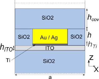
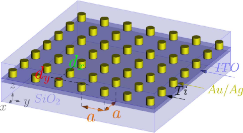
Figure 1: Schemes of the considered nanoparticles gratings.

Finally, the refractive indices of the different materials for the simulations are taken from weber2002handbook for SiO₂, johnson1972optical for gold, palik1998handbook for silver, and rakic1998optical for titanium.

II Numerical modeling

II.1 Finite Element Method formulation

The FEM formulation used in the present paper is described in demesy2010all . This numerical method allows calculation in the time-harmonic regime of the vector fields diffracted by any arbitrarily shaped crossed-grating embedded in a multilayered stack. The considered grating shown on Fig.1 is placed in an air superstrate (incident) medium with permittivity $\epsilon^{+}=1$. The SiO₂ substrate is considered as semi-infinite with permittivity $\epsilon^{-}$. All materials of the structure are considered to be non magnetic ($\mu_{r}=1$). The time-harmonic regime with a $\exp[-i\omega t]$ dependence is considered, where the frequency $\omega$ is related to a wavelength $\lambda=2\pi c/\omega$ in vacuum, $c$ being the speed of light in vacuum. The grating is illuminated with a plane wave $\boldsymbol{E}_{0}=\boldsymbol{A}_{0}\exp[i\,\boldsymbol{k}^{+}\cdot\boldsymbol{x}]$, where the wavevector $\boldsymbol{k}^{+}$ is defined by $\|\boldsymbol{k}^{+}\|={k}^{+}=k_{0}=\omega/c$ and the two angles $\theta_{0}\in[0,\pi/2]$ and $\psi_{0}\in[0,2\pi]$ ($\boldsymbol{k}^{+}$ is in the $xz$-plane if $\psi_{0}=0$ and $\boldsymbol{k}^{+}$ is in the $yz$-plane if $\psi_{0}=\pi/2$). This incident plane wave is p-polarized if the electric field is inside the incident plane (see left panel of Fig. 2) and s-polarized if the electric field is perpendicular to the incident plane (see right panel of Fig. 2).

                     

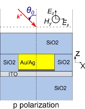
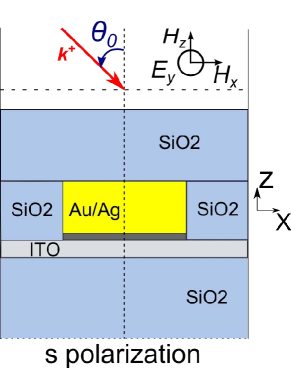
Figure 2: Scheme of the illumination conditions for wavevector $\boldsymbol{k}^{+}$ lying in the $xz$-plane ($\psi_{0}=0$).

We want to retrieve the total electromagnetic field $(\boldsymbol{E}\,,\boldsymbol{H})$ solution of the Helmholtz equation

$$\nabla\times\nabla\times\boldsymbol{E}+k_{0}^{2}\mu_{0}\epsilon\boldsymbol{E}=0\,,$$ (1)

where the diffracted field defined as $\boldsymbol{E}_{d}=\boldsymbol{E}-\boldsymbol{E}_{0}$ satisfies an outgoing wave condition, and where the field $\boldsymbol{E}$ is quasi-periodic along the two directions $x$ and $y$. The vector field $\boldsymbol{E}_{d}$ diffracted by the structure is calculated using the solution of an ancillary problem corresponding to the associated multilayered diffraction problem (without any diffractive element and with the same condition of illumination). This intermediate solution is then used as a known vectorial source term whose support is localized inside the diffractive element itself. Hence, the total field $\boldsymbol{E}$ of the structure is compound of three fields: i) the diffracted field $\boldsymbol{E}_{d}$ calculated using the FEM; ii) the incident plane wave $\boldsymbol{E}_{0}$; iii) the plane waves diffracted by the multilayer structure (the diffracted field associated to the ancillary problem which is compound of the transmitted and reflected waves of the multilayer structure). The total field $\boldsymbol{E}$ having Bloch-boundary conditions along the two directions of periodicity, the computation domain is then reduced to a single cell of the grating through the set $({k}_{x},{k}_{y})\equiv({k}^{+}_{x},{k}^{+}_{y})$ imposed by the incident plane-wave. [Note that the two-components wavevector $({k}_{x},{k}_{y})$ is the same in the whole structure with the grating periodicity: hence $({k}^{+}_{x},{k}^{+}_{y})$ is denoted by $({k}_{x},{k}_{y})$.] The implementation of those specific boundary conditions adapted to the FEM is described in nicolet2004modelling . As mentioned above, the diffracted field $\boldsymbol{E}_{d}$ should also satisfy an outgoing wave condition in the $z$-direction. Thus, a set of Perfectly Matched Layer (PML berenger1994perfectly ) are introduced in order to truncate the substrate and superstrate along the $z$ axis. Indeed, the diffracted field that radiates from the structure towards the infinite regions decays exponentially inside the implemented PML along the $z$ axis.

Once the values of the fields in the whole structure are obtained, they are used to compute a complete energy balance of the bi-periodic grating. It is based on i) the calculation of the diffraction efficiencies of each reflected and transmitted order along the two directions of periodicity of the gratings through a double Rayleigh expansion of the fields, and ii) the calculation of the normalized losses of each part of the diffractive (absorptive) element of the cell. This energy balance is then used to check the accuracy and self-consistency of the whole calculation as the sum of the different components of the energy balance should be equal to $1$.

The described method has been implemented into the following FEM free softwares: Gmsh geuzaine2009gmsh as a mesh generator and visualization tool, and GetDP dular1998general as a Finite Element Library. Numerous comparisons with the Fourier Modal Method LiFMM have been performed to check the accuracy of the present FEM method.

II.2 Comparison with measurements

Samples have been fabricated in order to check the relevance of the numerical tool. We use a commercial SiO₂ substrate covered by a 40 nm ITO layer. This ITO layer is used to evacuate charges during the lithography process. On this ITO thin film, a 4 nm titanium adhesion layer and a 30 nm gold film were deposited by electron beam evaporation. The gold nanocylinders are then realized by electron beam lithography. Scanning Electron Microscopy (SEM) imaging of the realized gratings are then performed and allow measurements of dimensions of the realized elliptical nanocylinders. Three gold nanocylinders gratings with different square periodicities have been fabricated: S1 ($a=200$ nm), S2 ($a=250$ nm) and S3 ($a=300$ nm).

	$a$	$d_{x}$	$d_{y}$
S1	$200$ nm	$91$ nm	$129$ nm
S2	$250$ nm	$87$ nm	$125$ nm
S3	$300$ nm	$84$ nm	$122$ nm

Table 1: Dimensions of cylinders of the three fabricated structures.

The elliptical diameters of nanocylinders for the three fabricated structures S1–S2–S3 are approximately $d_{x}\sim 80$ nm and $d_{y}\sim 120$ nm (see table 1 for the exact dimensions). Figure 3 shows a scheme and a SEM imaging of one of these gratings.

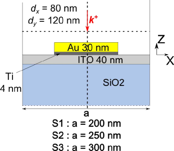
Figure 3: Scheme and SEM imaging of the fabricated structures S1–S2–S3.

The optical characterization of the samples is based on the measurement of transmission. A polychromatic source (Xe lamp) illuminates the samples through a monochromator and a polarizer. The source illuminating the samples is then almost monochromatic (with a wavelength from 400 nm to 1100 nm) and is linearly polarized. The transmission measurement is then performed with a home-made angulo-spectral optical reflectivity and transmissivity bench. Notice that this transmission measurement is normalized with respect to transmission for the bare SiO₂ substrate.

Transmission measurements have been performed for an incident beam in normal incidence with electric field polarized along the $y$-direction (s-polarisation) and the $x$-direction (p-polarisation) for wavelengths ranging from $500$ nm to $1100$ nm. These measurements are compared with the simulation results, where the gratings transmission efficiencies have been also normalized by the transmission of the bare SiO₂ substrate. Notice that the Au refractive index considered in these simulations for comparison is determined from measurements on the samples (there is a small difference from datas in johnson1972optical ).

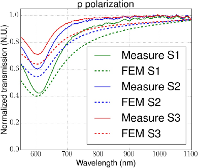
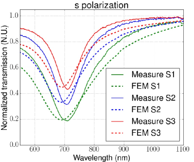
Figure 4: Comparison between the FEM results (dashed) and the measurements (line) in transmission for the three fabricated samples S1–S2–S3 .

Figure 4 shows excellent qualitative and quantitative agreement, and thus the relevance of the numerical tool employed to design plasmonic filters. The small remaining differences between the measurements and calculations can be attributed to the deviations in the shape of the fabricated cylinders, for example slanted walls or rounded corners.

III Parametric analysis and design of filtering properties

In this section, the influence of the different parameters of the system (nature of the metal, geometric parameters and illumination polarization) is analyzed in the case of an illumination with oblique incidence ($\theta_{0}=45^{\circ}$). This analysis is used to design an optimized structure for filtering properties. Here, the challenges are to obtain a choice of resonances in the visible spectrum with a minimum of optical losses or a maximum of averaged transmission.

From results presented in the previous section, it appears that structures of Au nanocylinders lead to resonances around 700 nm. Hence, Ag nanocylinder are considered in subsection 3.A to address the whole visible spectrum for the reflectivity peaks. Next, in subsection 3.B, the presence of absorption is analyzed starting from the reference structures S1–S2–S3 of Au nanoparticles. Finally, in subsection 3.C, optimized structures are proposed.

III.1 Influence of the cylinder diameters and of the incident polarization on the resonance wavelength.

The geometries considered in this subsection 3.A are similar to the ones of subsection 2.B (see Fig. 5) with the same ITO and Ti layers. The differences are: a $300$ nm SiO₂ cover layer in order to prevent the oxidation of the Ag nanocylinders; square periodicity of the gratings fixed to $a=200$ nm; Ag elliptical nanocylinders with axes $d_{x}$ fixed to $100$ nm and $d_{y}$ varying from $100$ nm to $180$ nm with a $20$ nm pitch (structures of type S4). Here, Ag nanocylinders have been introduced in order to address the whole visible spectrum with plasmonic resonances.

            

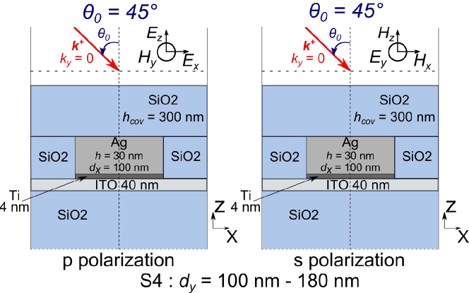
Figure 5: Scheme of the structure S4 for the considered conditions of illumination.

Simulations are performed for a plane wave for a wavevector lying in the $xz$-plane ($k_{y}=0$), and the angle of incidence with respect to the normal of the substrate is $\theta_{0}=45^{\circ}$. Both polarizations are considered (see Fig. 5). The simulations are performed for wavelengths spanning the visible range (380 to 780 nm). Fig. 6 shows the transmission efficiency in the specular order for the various $d_{y}$ diameters, for p and s polarizations.

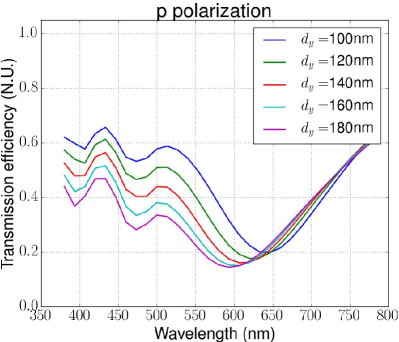
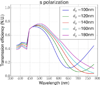
Figure 6: Efficiency in the transmission specular order for the group of structures S4.

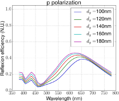
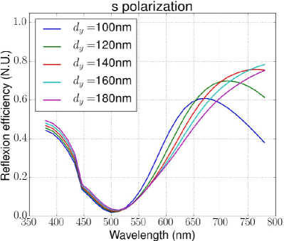
Figure 7: Efficiency in the reflexion specular order for the group of structures S4.

The corresponding efficiencies in the reflexion specular order are reported in Fig. 7. In the present case of an incident plane wave with wavevector lying in the $xz$-plane ($k_{y}=0$), when the plane wave is p-polarized, the electric field “sees” the small axis $d_{x}$ of the elliptical nanocylinder while, when the plane wave is s-polarized, the electric field “sees” the large axis $d_{y}$. One can observe in Figs. 6 and 7 that the resonance occuring for p polarization is at lower wavelength and less efficient that the one that occurs for s polarization. The more the incident electric field meets a high quantity of metal, the more the resonance is pronounced and redshifted. Also, in the two cases of polarizations, increasing $d_{y}$ broadens the reflexion peaks, which is coherent with an increasing quantity of metal. In the same time while increasing $d_{y}$, one can observe that the reflexion peak in p polarization is blueshifted while the one in s polarization is redshifted. Hence the two resonances in the two polarizations are not totally independent, but the general tendencies described above remain valid. These effects may allow us to manipulate the resonances observed in those elliptical nanocylinders gratings and to select wavelengths for which the reflexion peaks occur depending on the plane of incidence of the waves and their polarization. Hence the first challenge to obtain a resonance at the desired wavelength in the whole visible spectrum might be addressed.

III.2 Absorption and influence of the geometrical parameters

The second challenge is to reduce the absorption in order to obtain a high transmission when averaged on the whole visible spectrum. The influence of the quantity of metal is thus investigated in detail.

As a preliminary, we observe that, from the simulated total energy balance obtained for structure S2 (see Fig. 8), losses are important inside the ITO and Ti layers.

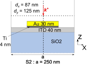
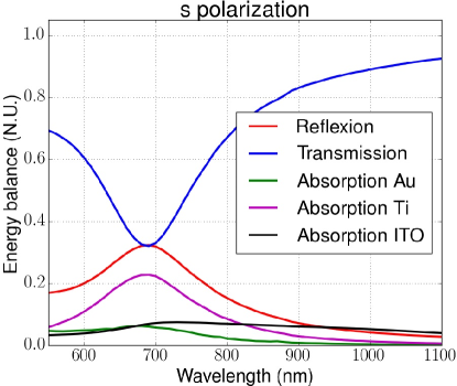
Figure 8: Decomposition of the total energy balance for s-polarization for the structure S2.

Since these materials play no role in the filtering function, suppressing ITO and Ti layers should be addressed in order to reduce Joule losses. From now, the investigation is performed with gold nanocylinders gratings directly deposited on the SiO₂ substrate.

                     

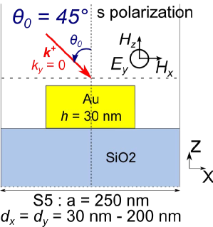
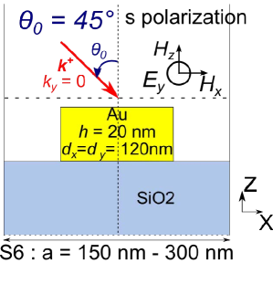
Figure 9: Scheme of the structures S5 (left panel) and S6 (right panel).

The influence of the quantity of metal is investigated by increasing the filling fraction of metal using two groups of structures. For the first group of structures S5 (left panel of Fig. 9), the size of the nanocylinders is increased for a fixed lattice constant $a$ and, conversely, the second group of structures S6 (right panel of Fig. 9), the size of the lattice constant $a$ is increased for a fixed nanocylinder dimension. Also, to simplify the number of parameters of influence, nanocylinders with circular cross section are considered here. The plane wave illuminating the structures has wavevector lying in the $xz$-plane ($k_{y}=0$) with an angle of incidence fixed to $\theta_{0}=45^{\circ}$, and is s polarized.

First the influence of the nanocylinder diameter on the total energy balance spectrum is analyzed. Notice that the propagative diffraction efficiencies higher than the $(0,0)$ specular orders are omitted since they are found to be negligible. The square pitch of the grating is fixed with $a=250$ nm, the gold nanocylinder height is fixed to $h=30$ nm, and their diameters vary from 30 to $200$ nm with $10$ nm pitch (group of structures S5). The left panel of Fig. 10 shows the reflexion efficiency in the specular order on the visible range ($380$ nm – $780$ nm) as a function of the nanocylinder diameter.

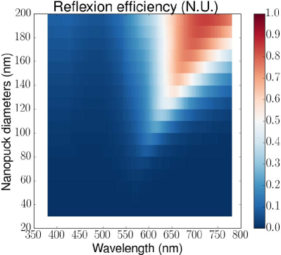
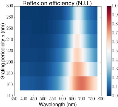
Figure 10: Left panel: Reflexion efficiency in the specular order for structures S5. Right panel: Reflexion efficiency in the specular order for structures S6.

One can observe that as the nanocylinder diameter increases, the reflexion peak intensity is magnified, redshifted and broadened. Again, one can check the possibility to choose the operating wavelength of the filter by selecting the appropriate diameter.

Second, the influence of the lattice constant $a$ on the total energy balance spectrum is analyzed. The nanocylinder geometry is then fixed with a height $h=20$ nm and a diameter $d_{x}=d_{y}=120$ nm. The square periodicity $a$ is now spanning the range (150 nm – 300 nm) with a 25 nm pitch (group of structures S6). The configuration of illumination remains unchanged (incident angle of $45^{\circ}$, $k_{y}=0$, s polarization). The right panel of Fig. 10 presents the spectrum of the reflexion efficiency in the specular order over the visible range ($380$ nm – $780$ nm) as a function of the lattice constant $a$. For fixed nanocylinder dimensions, increasing the grating square periodicity leads to slight variations of the central wavelength of the reflectivity peaks, which confirms that the resonance frequency is mainly governed by the particle diameter. Moreover, the intensity decreases and the peak is sharpened with the increase of the gratings periodicity. This result is fully consistent with the study of the influence of diameter.

Combination of these two parametric investigations leads to the following conclusions: i) the resonance frequency is mainly governed by the nanocylinder dimensions; ii) the ratio of the nanocylinder cross section surface over the lattice unit cell surface $a^{2}$ mainly governs the resonance intensity and absorption.

Before to present optimized structures, it is stressed that, in the configurations S5 and S6, efficient reflectivity peaks occurs for wavelengths around $650$ nm. If the structure is embedded into SiO₂ (like for structures S2 in section 2), then the observed peak in reflexion is redshifted and will occur only in the extreme red part of the visible spectrum, around $700$ nm (for structures S2). Thus, as conclusion iii), it appears necessary to consider the solution based on Ag proposed in the subsection 3.A to blueshift the resonances, since plasma frequency of Ag occurs at lower wavelengths. Finally, as pointed out in the preliminaries of this subsection 3.B, high absorption appears in ITO and Titanium layers (Fig. 8) and thus the optimization should be performed for nanocylinders standing directly on SiO₂ substrate (conclusion iv).

III.3 Optimized design with silver elliptical nanocylinders

In this section, we propose two different designs of silver elliptical nanocylinders gratings embedded in SiO₂ leading to peaks in the specular reflectivity in the visible range. The elliptical cross section of the nanocylinders allows two different peaks at two different wavelengths for a unique structure, depending on the polarization of illumination. The proposed filters possess also properties of global transparency on the visible spectrum.

               

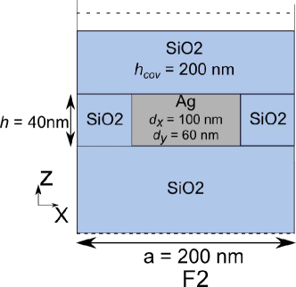
Figure 11: Schemes of the optimized filters F1 (left panel) and F2 (right panel).

The first proposed filter F1 is constituted of nanocylinders of $30$ nm height (left panel of Fig. 11). The ellipse diameters are $d_{x}=80$ nm and $d_{y}=60$ nm. The grating is embedded into SiO₂ (the substrate is SiO₂ and a SiO₂ cover layer of $200$ nm is added) and the square periodicity $a$ of the grating is fixed to $200$ nm. The incident wavevector lies either in the $xz$-plane ($k_{y}=0$) or in the $yz$-plane ($k_{x}=0$), with an angle of incidence fixed to $\theta_{0}=45^{\circ}$, and both p and s polarizations are considered. Figure 12 shows the different components of the energy balance for the filtering structure F1.

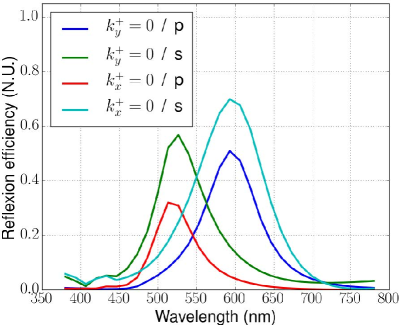
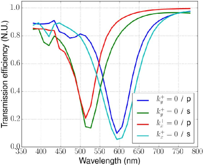
Figure 12: Reflexion (left panel) and transmission (right panel) efficiencies in the specular order for the structure F1.

This geometry leads to reflexion peaks in the specular order centered at two different wavelengths (525 nm and 590 nm) depending on the incidence plane and polarization.

The second proposed filter F2 is made of nanocylinders with $40$ nm height (right panel of Fig. 11). The ellipse diameters are $d_{x}=100$ nm and $d_{y}=60$ nm. The grating is embedded into SiO₂ (cover layer of $200$ nm and substrate). The square periodicity $a$ of the grating remains $200$ nm, and the illumination conditions are the same than for F1.

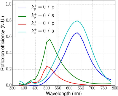
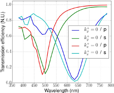
Figure 13: Reflexion (left panel) and transmission (right panel) efficiencies in the specular order for the structure F2.

Figure 13 shows the different components of the energy balance for grating F2. Here, reflexion peaks are obtained at the two different wavelengths $520$ nm and $633$ nm. In both cases the averaged transmission over the whole visible spectrum is above 64%, which ensures correct transparency. This is confirmed by the absorption spectra of the two structures reported on Fig. 14.

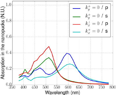
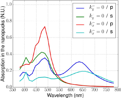
Figure 14: Absorption in the nanocylinders for structures F1 (left panel) and F2 (right panel).

IV Homogenization of nanocylinders structures

In this section, the properties of nanoparticles gratings are modeled using Maxwell-Garnett homogenization. A detailed discussion on this homogenization of elliptic nanoparticles can be found in Hom96 , and more recently in Hom09 .

In the present case, we consider anisotropic inclusions for which the effective permittivity components $\epsilon_{j}$ $(j=x,y,z)$ are given by:

$$\epsilon_{j}-\epsilon_{m}=\epsilon_{m}\,\displaystyle\frac{f(\epsilon_{p}-\epsilon_{m})}{\epsilon_{m}+L_{j}(\epsilon_{p}-\epsilon_{m})}\left[1-L_{j}\,\displaystyle\frac{f(\epsilon_{p}-\epsilon_{m})}{\epsilon_{m}+L_{j}(\epsilon_{p}-\epsilon_{m})}\right]^{-1}\,.$$ (2)

Here, $\epsilon_{p}$ and $\epsilon_{m}$ are the permittivity of particles and surrounding medium respectively, $f$ is the filling fraction of metal, and $L_{j}$ are the components of the depolarization dyadic in the corresponding axis $(j=x,y,z)$. We consider a cylindrical inclusion of elliptical cross section oriented in the z-direction embedded into a rectangular box. The height of the rectangular box is equal to the height $2h$ of the cylinder (see Fig. 15). The basis of the rectangular box is the square unit cell of lattice. Hence the filling fraction $f$ is just the ratio of the cylinder section (an ellipse of radius $R_{x}=d_{x}/2$ and $R_{y}=d_{y}/2$) with respect to $a^{2}$, i.e. $f=\pi R_{x}R_{y}/a^{2}$.

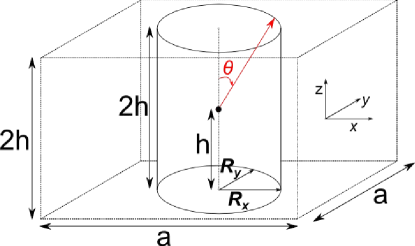
Figure 15: Scheme of the considered unit cell.

The calculation of the depolarization components is reported in the appendix, in the both cases of cylinders with circular (appendix A) and elliptic (appendix B) cross section. After computing the different depolarization factors, the effective permittivity components are calculated from Eq. (2).

This effective model has been applied to a square unit cell ($a=200$ nm) composed of a silver cylinder of elliptical cross section with radii $R_{x}=40$ nm and $R_{y}=30$ nm and height $2h$=30 nm. The considered background medium is SiO₂. Hence, this unit cell represents the one of the grating corresponding to the structure F1. The following depolarization components are obtained using Eqs. (18,22): $L_{x}=0.16$, $L_{y}=0.24$ and $L_{z}=0.60$. The corresponding effective anisotropic relative permittivity components are reported in left panel Fig. 16. One can check that the effective permittivity components show resonances around 480 nm and 575 nm.

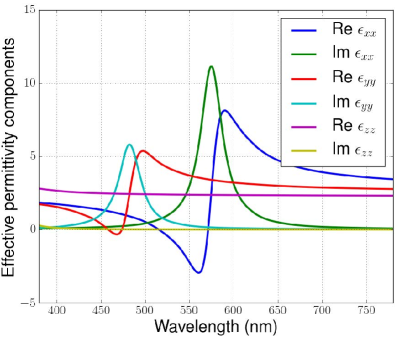
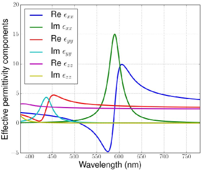
Figure 16: Effective anisotropic relative permittivity components for the unit cell of structures F1 (left panel) and F2 (right panel).

Next the multilayer corresponding to the structure F1 is considered. The multilayer is composed of (from top to bottom): 1) an incident medium (air); 2) a 200 nm SiO₂ layer corresponding to the cover layer; 3) a 30 nm homogenized layer of effective permittivity given in left panel of Fig. 16 corresponding to the grating; 4) a SiO₂ substrate. The reflexion and transmission coefficients have been calculated for an incident plane wave with incident wavevector that lies either in the $xz$-plane ($k_{y}=0$) either in the $yz$-plane ($k_{x}=0$), with an angle of incidence fixed to $\theta_{0}=45^{\circ}$, and for wavelengths spanning the visible range. Both p and s polarizations have been considered and compared to the rigorous FEM calculation of subsection 3.III.3. This comparison is shown in Fig.17.

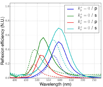
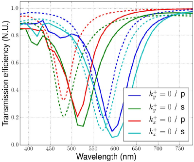
Figure 17: Reflexion (left panel) and transmission (right panel) efficiencies of structure F1 obtained with the rigorous FEM calculation (line) and with the homogenization model (dashed).

The same reasoning has been applied to the structure F2 and leads to the following depolarization components: $L_{x}=0.16$, $L_{y}=0.32$ and $L_{z}=0.52$. The corresponding effective relative permittivity is plotted in right panel of Fig.16, and presents resonances around 440 nm and 575 nm. The reflexion and transmission coefficients for the effective multilayer are compared to FEM results in Fig.18.

One can observe that the homogenization leads to resonances which are in relative agreement with the rigorous FEM results, except a shift about 50 nm for the resonance wavelength. This shift can be attributed to the effect of the finite size of particles, since it can be checked numerically that this shift decreases together with the particle size. These resonances are both present in the effective permittivity components and the spectra of transmission and reflexion. Hence these homogenization results provide useful tendencies with much faster computation time, and can be used to design filtering properties.

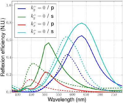
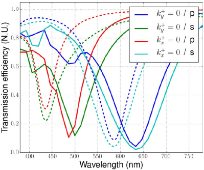
Figure 18: Reflexion (left panel) and transmission (right panel) efficiencies of structure F2 obtained with the rigorous FEM calculation (line) and with the homogenization model (dashed).

Notice that a similar homogenization model can be derived in the more complex situation were the particles stand directly on a substrate, without cover layer (for instance structures S5 or S6). For such case, the calculation of the depolarization factors is given in the appendix C.

V Diffraction by a single nanocyclinder

In this last section, the contribution of the single nanoparticle to the electromagnetic behavior of the grating is analyzed. To that end, the problem of plane wave scattering by a single nanoparticle is solved numerically using the FEM via an approach similar to Sec. II.A changing Bloch-Floquet boundary conditions to perfectly matched layers. Finally, a multipole expansion of the diffracted field is performed and discussed.

Consider a non magnetic scatterer of arbitrary shape, relative permittivity $\varepsilon_{s}^{b}$ embedded in a transparent non magnetic homogeneous background of relative permittivity $\varepsilon_{r}^{b}$. We denote by $\varepsilon_{r}(\mathbf{x})$ the piecewise constant function equal to $\varepsilon_{s}^{b}$ within the scatterer and $\varepsilon_{r}^{b}$ elsewhere. The scatter is enlighten by a plane wave of arbitrary incidence and polarization $\boldsymbol{E}_{0}$. This incident field, i.e. the field in absence of the scatterer is the solution of the vector Helmholtz propagation equation in the resulting homogeneous medium:

$$\nabla\times\nabla\times\boldsymbol{E}_{0}(\mathbf{x})+k_{0}^{2}\,\varepsilon_{r}^{b}\,\boldsymbol{E}_{0}(\mathbf{x})=\mathbf{0}\,.$$ (3)

We are looking for the total field $\boldsymbol{E}$, resulting from the electromagnetic interaction of the scatterer and the incident field, which is the solution of the Helmholtz equation:

$$\nabla\times\nabla\times\boldsymbol{E}(\mathbf{x})+k_{0}^{2}\,\varepsilon_{r}(\mathbf{x})\,\boldsymbol{E}(\mathbf{x})=\mathbf{0}\,.$$ (4)

The field diffracted or scattered by the object is defined as $\boldsymbol{E}_{d}:=\boldsymbol{E}-\boldsymbol{E}_{0}$. Combining Eqs. (3, 4) allows to reformulate scattering problem to a radiation problem. The scattered field now $\boldsymbol{E}_{d}$ satisfies the following propagation equation :

$$\nabla\times\nabla\times\boldsymbol{E}_{d}(\mathbf{x})+k_{0}^{2}\,\varepsilon_{r}(\mathbf{x})\,\boldsymbol{E}_{d}(\mathbf{x})=k_{0}^{2}\,(\varepsilon_{r}(\mathbf{x})-\varepsilon_{r}^{b})\,\boldsymbol{E}_{0}(\mathbf{x})\,$$ (5)

such that $\boldsymbol{E}_{d}$ satisfies a radiation condition. The right hand side can be viewed as a volume (current) source term with support the scatterer itself, $\varepsilon_{r}(\mathbf{x})-\varepsilon_{r}^{b}$ being equal to $\varepsilon_{s}^{b}-\varepsilon_{r}^{b}$ inside the scatterer and 0 elsewhere.

The scattered field $\boldsymbol{E}_{d}$ can be expanded on the basis of outgoing vector partial waves $(\mathsf{\mathbf{M}}_{n,m}^{(+)},\mathsf{\mathbf{N}}_{n,m}^{(+)})$ built upon the vector spherical harmonics $(\mathsf{\mathbf{X}}_{n,m},\mathsf{\mathbf{Y}}_{n,m},\mathsf{\mathbf{Z}}_{n,m})$ following the framework and conventions described in detail in Stout06I ; Stout06II :

$$\mathsf{\mathbf{M}}_{n,m}^{(+)}(k\mathbf{r}) = h_{n}^{(+)}(kr)\,\mathsf{\mathbf{X}}_{n,m}(\theta,\varphi)$$ (6)

$$\mathsf{\mathbf{N}}_{n,m}^{(+)}(k\mathbf{r}) = \frac{1}{kr}\displaystyle\left[\sqrt{n(n+1)}\,h_{n}^{(+)}(kr)\,\mathsf{\mathbf{Y}}_{n,m}(\theta,\varphi)\right.$$

$$+ \xi^{\prime}(kr)\,\mathsf{\mathbf{Z}}_{n,m}(\theta,\varphi)\displaystyle\bigg{]}$$

The so-called multipole expansion is finally given by :

$$\boldsymbol{E}_{d}(\mathbf{r})=\displaystyle\sum_{n=1}^{n_{\mathsf{max}}}\sum_{m=-n}^{m}f^{(h)}_{n,m}\,\mathsf{\mathbf{M}}_{n,m}^{(+)}(k\mathbf{r})+f^{(e)}_{n,m}\,\mathsf{\mathbf{N}}_{n,m}^{(+)}(k\mathbf{r})\,\,$$ (8)

where $f^{(h)}_{n,m}$ and $f^{(e)}_{n,m}$ can be numerically computed on any sphere of radius $R$ englobing the scatterer :

$$f^{(e)}_{n,m} = \frac{kR}{\xi^{\prime}(kR)}\displaystyle\int_{0}^{2\pi}\int_{0}^{\pi}\boldsymbol{E}_{d}(R,\theta,\varphi)\cdot\mathsf{\mathbf{Z}}_{n,m}^{\star}(\theta,\varphi)\,\mathsf{d}\theta\,\mathsf{d}\varphi$$ (9)

$$f^{(h)}_{n,m} = \frac{kR}{h_{n}^{(+)}(kR)}\displaystyle\int_{0}^{2\pi}\int_{0}^{\pi}\boldsymbol{E}_{d}(R,\theta,\varphi)\cdot\mathsf{\mathbf{X}}_{n,m}^{\star}(\theta,\varphi)\,\mathsf{d}\theta\,\mathsf{d}\varphi$$ (10)

Note that $\boldsymbol{E}_{d}$ in Eqs. (9) and (10) is expressed from the FEM inherited cartesian coordinates to spherical coordinates. This expansion is the classical way to obtain the far field radiation pattern of antennas. It would require major adjustments to take into account the substrate and superstrate. First of all, let us state that the resonant phenomena described in the previous section do not depend on the close vicinity of the interface. Figure 19 shows the reflectivity of silver nanocylinders grating of the optimized structure F1, when embedded in an homogeneous infinite $\mathrm{SiO}_{2}$ background. In this simplified model, the $\theta_{0}$ incidence is adjusted to compensate for the missing refraction at $\mathrm{SiO}_{2}$ interface $\theta_{0}=\mathrm{arcsin}(\mathrm{sin}(45^{\circ})/n_{\mathrm{SiO}_{2}})\approx 29^{\circ}$. The same four resonances as in Fig. 14 are obviously excited with $\theta=29^{\circ}$ depending on the plane of incidence (compare dashed and plain lines in Fig. 19). The only noticeable difference in s-polarization case (see green and cyan lines in Fig. 19) can be partly explained by the fact that at $45^{\circ}$ incidence, reflexion on a bare silica diopter is $\sim 8.3\%$ in s-polarization (while only $\sim 0.5\%$ in p-polarization, due to the Brewster effect).

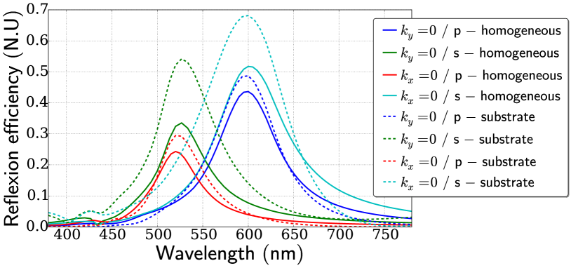
Figure 19: (Dashed lines) Reflexion efficiency in the specular order for the structure F1 (same as left panel of Fig. 12). (Plain lines) Grating of silver nanocylinders of same dimensions as in optimized structure F1, but embedded in homogeneous SiO₂ background. Reflexion peaks in both panels are very similar.

Consider now the single scatterer case. First of all, the only non negligible terms in expansion Eq. (8) correspond to electric dipoles whatever the considered incidence. All higher electric orders and all magnetic orders are at least 50 fold lower in magnitude than the dipolar electric ones over the whole visible spectrum. As shown in Fig. 20(a) and 20(b) for $k_{y}=0$, i.e. when the plane of incidence contains the $r_{x}$-axis of the ellipse, two resonant scenarii occur depending on the incident polarization. With p-polarization [Fig. 20(a)], the incident electric field lies within the plane of incidence, and two electric multipoles dominate the far field scattered power, corresponding to induced electric dipoles of moments along $Ox$ (see $f^{(e)}_{1,\pm 1}$) and $Oz$ (see $f^{(e)}_{1,0}$). Heuristically, the incident electric field indeed only sees two characteristic dimensions of the scatterer, i.e. the height $h$ of the elliptic nanocylinder and its greater diameter $2r_{x}$. With $s$-polarization, the only induced dipole present is along $Oy$, corresponding to the fact that the electric field now only sees the smaller diameter $2r_{y}$. The larger radius [Fig. 20(a)] leads to a redshifted resonant response of the particle, as already observed for gold circular cylinders (see Fig. 10). The same considerations hold for $k_{x}=0$ as depicted in Fig. 20(c) and 20(d). Electric field maps of the periodic and isolated cases are very similar in spite of the rather small 200 nm bi-period, which further confirms the weak coupling between the elliptic nanocylinders. Above 450 nm, the subwavelength bi-periodicity selects only the specular propagation direction among all by constructive interferences.

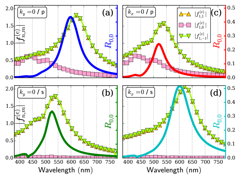
Figure 20: reflexion of the periodic structure compared to multipolar coefficients of the isolated scatterer for incidence $\theta_{0}=29^{\circ}$, with (a) $k_{y}=0$ and p-polarization, (b) $k_{x}=0$ and p-polarization , (c) $k_{y}=0$ and s-polarization , (d) $k_{x}=0$ and s-polarization.

VI Conclusions

We have shown the possibility to design efficient reflective filters with selective wavelength mirror properties together with global transparency over the visible range. A numerical tool based on the FEM has been used to analyze the behavior of nanoparticles gratings, and comparison between numerical and experimental results has been performed. Two optimized filters with two operating wavelengths depending on the polarization have been proposed. It has been shown that Maxwell-Garnett homogenization can be used to model the considered structures. Also, the calculation of the radiation by a single nanoparticle has shown that the diffractive properties of the considered systems are governed by a single isolated particle.

Whereas the main principle has been demonstrated, the full structure can be improved by several manners in order to increase the reflectivity and transmission. Especially, fabrication can be done now without ITO conductive layer and without Ti attaching layer. This should significantly reduce absorption. Besides, since the diffractive properties are governed by a single isolated particle, the same properties can be obtained with periodic or aperiodic structures as along as the size and the density of the nanoparticles are the same. This may also considerably ease the fabrication on large surfaces.

These promising results pave the way of smart windows and could find some innovative applications in transport industry such as automotive or aeronautic sectors for displays, human-machine interfaces and sensors.

Funding Information

This work has been supported by the ANR funded project PLANISSIMO (ANR-12-NANO-0003) and by the french RENATECH network.

VII appendix

VII.1 Depolarization dyadic for circular cylinders

The calculation of depolarization dyadic components associated with a finite circular cylinder is recalled. Let $V$ be the volume of a cylinder of height $2h$ and radius $R$, and let $\boldsymbol{r}$ be the vector of coordinates $(x,y,z)$ with the origin $\boldsymbol{r}=0$ at the center of the cylinder. Then, the dimensionless depolarization dyadic at the center of the cylinder is formally given by

$$L=-\displaystyle\int_{V}d\boldsymbol{r}\,\nabla\nabla\displaystyle\frac{1}{4\pi|\boldsymbol{r}|}\,.$$ (11)

This expression has to be considered carefully since a singularity is present at the origin. This difficulty is fixed by splitting the integral above into a first integral over a small sphere $B_{0}$ and a second integral over the remaining volume $V\setminus B_{0}$. Next, using that the integral over $B_{0}$ is just $1/3$ of the unit dyadic $U$, we have

$$L=\displaystyle\frac{1}{3}U-\displaystyle\int_{V\setminus B_{0}}d\boldsymbol{r}\,\nabla\nabla\displaystyle\frac{1}{4\pi|\boldsymbol{r}|}\,.$$ (12)

Now, the Green-Ostrogradski theorem can be applied. Let $S$ and $S_{0}$ be the surfaces of the cylinder $V$ and the sphere $B_{0}$ respectively. The expression above becomes

$$L=\displaystyle\frac{1}{3}U-\displaystyle\int_{S}ds\,\boldsymbol{n}\nabla\displaystyle\frac{1}{4\pi|\boldsymbol{r}|}\,+\displaystyle\int_{S_{0}}ds\,\boldsymbol{n}\nabla\displaystyle\frac{1}{4\pi|\boldsymbol{r}|}\,.$$ (13)

where $ds$ is the infinitesimal surface element and $\boldsymbol{n}$ is the outgoing normal of the surfaces. Since the last term is just $U/3$, the expression reduces to

$$L=-\displaystyle\int_{S}ds\,\boldsymbol{n}\nabla\displaystyle\frac{1}{4\pi|\boldsymbol{r}|}=\displaystyle\int_{S}ds\,\boldsymbol{n}\displaystyle\frac{\boldsymbol{r}}{4\pi|\boldsymbol{r}|^{3}}\,.$$ (14)

Finally, using the symmetries of the cylinder, it is found that the component $L_{z}\equiv L_{zz}$ of the dyadic is given by the integration over the two horizontal disks at the top and bottom of the cylinder:

$$L_{z}=2\displaystyle\int_{0}^{R}dr\,\displaystyle\int_{0}^{2\pi}rd\phi\,\displaystyle\frac{h}{4\pi(h^{2}+r^{2})^{3/2}}=1-\cos\theta\,.$$ (15)

As to the components $L_{x}\equiv L_{xx}$ and $L_{y}\equiv L_{yy}$ ($L_{y}=L_{x}$ by symmetry), they are provided by the integration over the vertical face of the cylinder:

$$L_{x}=\displaystyle\int_{-h}^{h}dz\,\displaystyle\int_{0}^{2\pi}Rd\phi\,\displaystyle\frac{R\cos^{2}\phi}{4\pi(z^{2}+R^{2})^{3/2}}=\displaystyle\frac{1}{2}\cos\theta\,.$$ (16)

Hence the well known expressions yaghjian1980electric ; van2007electromagnetic have been retrieved.

VII.2 Depolarization dyadic for elliptic cylinders

In this subsection, $V$ and $S$ are the volume and the surface respectively of a cylinder with elliptic cross section of height $2h$ and radii $R_{x}$ and $R_{y}$. All the procedure performed in the circular case remains correct until equation (14). Similarly to the previous case, using the symmetries of the elliptic cylinder, it is found that the component $L_{z}$ is given by the integration over the two horizontal surfaces $S_{e}$ defined by

$$S_{e}=\{(x,y)\,|\,x^{2}/R_{x}^{2}+y^{2}/R_{y}^{2}\leq 1\,\}\,.$$ (17)

Then the depolarization component in the $z$ direction is

$$L_{z}=2\displaystyle\int_{S_{e}}dx\,dy\,\displaystyle\frac{h}{4\pi(h^{2}+x^{2}+y^{2})^{3/2}}\,,$$ (18)

which requires numerical integration to determine its value. Again using the symmetries of the cylinder, it is deduced that the depolarization factors $L_{x}$ and $L_{y}$ are provided by the integration over the vertical face of the cylinder. The vector $\boldsymbol{r}$ describing this surface is (the third component $z$ can be omitted)

$$\boldsymbol{r}=\left(\begin{array}[]{c}R_{x}\cos\phi\\ R_{y}\sin\phi\end{array}\right)\quad\Longrightarrow\quad\displaystyle\frac{d\boldsymbol{r}}{d\phi}=\left(\begin{array}[]{c}-R_{x}\sin\phi\\ R_{y}\cos\phi\end{array}\right)$$ (19)

and the unit normal $\boldsymbol{n}$, orthogonal to $d\boldsymbol{r}/d\phi$, is then

$$\boldsymbol{n}=\displaystyle\frac{1}{\sqrt{R_{x}^{2}\sin^{2}\phi+R_{y}^{2}\cos^{2}\phi}}\left(\begin{array}[]{c}R_{y}\cos\phi\\ R_{x}\sin\phi\end{array}\right)\,.$$ (20)

Then the tensor product of the two vectors $\boldsymbol{n}$ and $\boldsymbol{r}$ is given by

$$\boldsymbol{n}\boldsymbol{r}=\displaystyle\frac{1}{\sqrt{R_{x}^{2}\sin^{2}\phi+R_{y}^{2}\cos^{2}\phi}}\left(\begin{array}[]{lr}\!\!\!R_{x}R_{y}\cos^{2}\phi&R_{x}^{2}\cos\phi\sin\phi\!\!\!\\ \!\!\!R_{y}^{2}\cos\phi\sin\phi&R_{x}R_{y}\sin^{2}\phi\!\!\!\end{array}\right)\!.$$ (21)

Finally, since $ds=dzd\phi\times|d\boldsymbol{r}/d\phi|$, the obtained expressions for the depolarization are:

$$\begin{array}[]{l}L_{x}=\displaystyle\int_{-h}^{h}dz\,\displaystyle\int_{0}^{2\pi}d\phi\,\displaystyle\frac{R_{x}R_{y}\cos^{2}\phi}{4\pi(z^{2}+R_{x}^{2}\cos^{2}\phi+R_{y}^{2}\sin^{2}\phi)^{3/2}}\,,\\[5.69054pt] L_{y}=\displaystyle\int_{-h}^{h}dz\,\displaystyle\int_{0}^{2\pi}d\phi\,\displaystyle\frac{R_{x}R_{y}\sin^{2}\phi}{4\pi(z^{2}+R_{x}^{2}\cos^{2}\phi+R_{y}^{2}\sin^{2}\phi)^{3/2}}\,.\end{array}$$ (22)

Numerical integration is required to obtain the values of these components.

VII.3 Depolarization dyadic for circular cylinders on a substrate

The case of a circular cylinder lying on a substrate is considered. The notations are the same as in the appendix A, with the origin $\boldsymbol{r}=0$ at the center of the cylinder of height $2h$. In addition, a substrate of relative permittivity $\epsilon^{-}$ is located in the half space $z<-h$ with its plane interface at the bottom circular face of the cylinder. Let $\epsilon(\boldsymbol{r})$ be the relative permittivity defining the environment of the cylinder: $\epsilon(\boldsymbol{r})=1$ if $z>-h$ and $\epsilon(\boldsymbol{r})=\epsilon^{-}$ if $z<-h$. The electrostatic potential $\Phi(\boldsymbol{r})$ created by a point source is the solution of

$$\nabla\cdot\epsilon(\boldsymbol{r})\nabla\Phi(\boldsymbol{r})=\delta(\boldsymbol{r})$$ (23)

Denoting $\boldsymbol{r}_{0}=2h\boldsymbol{e}_{z}$, the solution of the equation above is

$$\begin{array}[]{l}z>-h\,:\quad\Phi(\boldsymbol{r})=-\displaystyle\frac{1}{4\pi|\boldsymbol{r}|}-\displaystyle\frac{1-\epsilon^{-}}{1+\epsilon^{-}}\displaystyle\frac{1}{4\pi|\boldsymbol{r}+\boldsymbol{r}_{0}|}\,,\\[5.69054pt] z<-h\,:\quad\Phi(\boldsymbol{r})=-\displaystyle\frac{2}{1+\epsilon^{-}}\displaystyle\frac{1}{4\pi|\boldsymbol{r}|}\,.\end{array}$$ (24)

The depolarization dyadic is then given by an expression equivalent to equation (14):

$$L=-\displaystyle\int_{S}ds\,\boldsymbol{n}\nabla\Phi(\boldsymbol{r})\,.$$ (25)

Next, the calculation is similar to the one in the appendix A, with an additional term corresponding to the reflexion part of $\Phi(\boldsymbol{r})$. The resulting expression for the vertical component of the depolarization dyadic is

$$L_{z}=1-\cos\theta+\displaystyle\frac{1-\epsilon^{-}}{1+\epsilon^{-}}\displaystyle\frac{\cos\theta-\cos\theta_{1}}{2}\,,$$ (26)

where

$$\cos\theta=\displaystyle\frac{h}{\sqrt{h^{2}+R^{2}}}\,,\quad\cos\theta_{1}=\displaystyle\frac{3h}{\sqrt{(3h)^{2}+R^{2}}}\,.$$ (27)

The other components of the dyadic are

$$L_{x}=L_{y}=\displaystyle\frac{\cos\theta}{2}-\displaystyle\frac{1-\epsilon^{-}}{1+\epsilon^{-}}\displaystyle\frac{\cos\theta-\cos\theta_{1}}{4}\,.$$ (28)

This calculation can be extended to cylinders with elliptic cross section by following the procedure of appendix B.

References

- (1) N. Perney, J. J. Baumerg, M. E. Zoorob, M. D. Charlton, S. Mahnkopf, and C. M. Netti, “Tuning localized plasmons in nanostructured substrates for surface-enhanced raman scattering,” Opt. Express 14, 847 (2006).
- (2) J. N. Yih, Y. M. Chu, Y. C. Mao, W. H. Wang, F. C. Chien, C. Y. Lin, K. L. Lee, P. K. Wei, and S. J. Chen, “Optical waveguide biosensors constructed with subwavelength gratings,” Appl. Opt. 45, 1938 (2006).
- (3) K. Kumar, H. Duan, R. S. Hegde, S. C. W. Koh, J. N. Wei, and J. K. W. Yang, “Printing colour at the optical diffraction limit,” Nat. Nanotechnol. 7, 557 (2012).
- (4) G. Si, Y. Zhao, J. Lv, M. Lu, F. Wang, H. Liu, N. Xiang, T. J. Huang, A. J. Danner, J. Teng, and Y. J. Liu, “Reflective plasmonic color filters based on lithographically patterned silver nanorod arrays,” Nanoscale 5, 6243 (2013).
- (5) C. W. Hsu, B. Zhen, W. Qiu, O. Shapira, B. G. DeLacy, J. D. Joannopoulos, and M. Soljačić, “Transparent displays enabled by resonant nanoparticle scattering,” Nat. Commun. 5, 3152 (2014).
- (6) T. Xu, Y.-K. Wu, X. Luo, and L. J. Guo, “Plasmonic nanoresonators for high-resolution colour filtering and spectral imaging,” Nat. Commun. 1, 59 (2010).
- (7) B. Zeng, Y. Gao, and F. J. Bartoli, “Ultrathin nanostructured metals for highly transmissive plasmonic subtractive color filters,” Sci. Rep. 3, 2840 (2013).
- (8) G. Demésy, F. Zolla, A. Nicolet, and M. Commandré, “All-purpose finite element formulation for arbitrarily shaped crossed-gratings embedded in a multilayered stack,” J. Opt. Soc. Am. A 27, 878 (2010).
- (9) L. Li, “Fourier modal method,” in Gratings: Theory and Numeric Applications, Second Revisited Edition, Chap. 13, Editor E. Popov (Aix-Marseille Université, CNRS, Centrale Marseille, Institut Fresnel, 2014).
- (10) M. J. Weber, Handbook of optical materials, vol. 19 (CRC press, 2002).
- (11) P. B. Johnson and R. W. Christy, “Optical constants of the noble metals,” Phys. Rev. B 6, 4370 (1972).
- (12) E. D. Palik, Handbook of optical constants of solids, vol. 3 (Academic press, 1998).
- (13) A. D. Rakić, A. B. Djiurisic, J. M. Elazar, and M. L. Majewski, “Optical properties of metallic films for vertical-cavity optoelectronic devices,” Appl. Opt. 37, 5271 (1998).
- (14) A. Nicolet, S. Guenneau, C. Guezaine, and F. Zolla, “Modelling of electromagnetic waves in periodic media with finite elements,” J. Comput. Appl. Math. 168, 321 (2004).
- (15) J.-P. Berenger, “A perfectly matched layer for the absorption of electromagnetic waves,” J. Comput. Phys. 114, 185 (1994).
- (16) C. Geuzaine and J.-F. Remacle, “Gmsh: A 3-d finite element mesh generator with built-in pre-and post-processing facilities,” Int. J. Numer. Meth. Eng. 79, 1309 (2009).
- (17) P. Dular, C. Guezaine, F. Henrotte, and W. Legros, “A general environment for the treatment of discrete problems and its application to the finite element method,” IEEE Trans. Magn. 34, 3395 (1998).
- (18) N. A. Nicorovici and R. C. McPhedran, “Transport properties of arrays of elliptical cylinders,” Phys. Rev. E 54, 1945 (1996).
- (19) V. Mityushev, “Conductivity of a two-dimensional composite containing elliptical inclusions,” Proc. R. Soc. A 465, 2991 (2009).
- (20) B. Stout, M. Nevière, and E. Popov, “Mie scattering by an anisotropic object. part i: Homogeneous sphere,” J. Opt. Soc. Am. A 23, 1111 (2006).
- (21) B. Stout, M. Nevière, and E. Popov, “Mie scattering by an anisotropic object. part ii: Arbitrary-shaped object - differential theory,” J. Opt. Soc. Am. A 23, 1124 (2006).
- (22) A. D. Yaghjian, “Electric dyadic green’s functions in the source region,” Proc. IEEE 68, 248 (1980).
- (23) J. G. Van Bladel, Electromagnetic fields (John Wiley & Sons, 2007).