Higgs production within -factorization
with unintegrated gluon distributions
Abstract:
We present differential cross sections for Higgs boson and/or two-photon production from intermediate (virtual) Higgs boson within the formalism of -factorization. Resulting distributions for two photons from the Higgs boson are compared with recent ATLAS collaboration data. In contrast to a recent calculation the leading order contribution is rather small compared to the ATLAS experimental data ( transverse momentum and rapidity distributions). We include also higher-order contribution , and the contribution of the and exchanges. The mechanism gives a similar contribution as the mechanism. We argue that there is almost no double counting when adding and contributions due to different topology of corresponding Feynman diagrams. The final sum is comparable with the ATLAS two-photon data.
1 Introduction
The Higgs boson was discovered at the LHC [1]. It has been observed in a few decay channels. The and are particularly spectacular [2, 3, 4, 5].
After the discovery understanding the rapidity and transverse momentum distributions is particularly interesting. While the total cross section is well under control and was calculated in leading-order (LO), next-to-leading order (NLO) and even next-to-next-to-leading order (NNLO) approximation [6] the distribution in the Higgs boson transverse momentum is more chalanging.
It was advocated recently that precise differential data for Higgs boson in the two-photon final channel could be very useful to test and explore unintegrated gluon distribution functions (UGDFs) [7]. It was claimed very recently [8] that the -factorization formalism with commonly used UGDFs (Kimber-Martin-Ryskin (KMR) [9] and Jung CCFM [10]) gives a reasonable description of recent ATLAS data obtained at 8 TeV [11]. We perform similar calculation and draw rather different conclusions.
Here we report on our results from Ref.[12] obtained within -factorization approach where we presented several differential distributions for the Higgs boson and photons from the Higgs boson decay at = 8 TeV for various UGDFs from the literature.
There we have included both leading-order and next-to-leading order contributions. We shall critically discuss uncertainties and open problems in view of the recent ATLAS data.
2 A sketch of the formalism
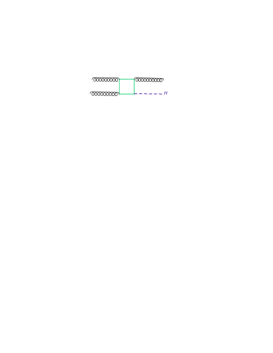
The leading-order mechanism of Higgs boson production in the -factorization is shown in Fig.1.
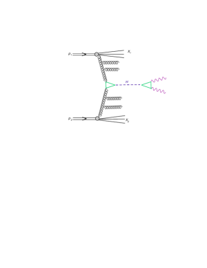
The leading-order diagram for Higgs boson production in the two-photon channel relevant for the -factorization approach.
In the -factorization approach the cross section for the Higgs boson production can be written somewhat formally as:
| (1) | |||||
where are so-called unintegrated (or transverse-momentum-dependent) gluon distributions and is (off-shell) cross section.
In Fig.2 we show next-to-leading order partonic subprocesses. While the processes with triangles are effectively included in a calculation related to the diagram shown in Fig.1, the diagrams with boxes (much larger contributions) have to be included extra.
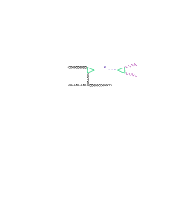
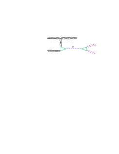
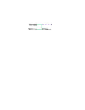
QCD NLO subprocesses with triangles (upper line) and boxes (lower line).
In the collinear approximation the corresponding cross section differential in Higgs boson rapidity (), associated parton rapidity () and transverse momentum of each of them can be written as:
| (2) | |||||
The indices in the formula above number both quarks ( 0) and antiquarks ( 0). Only three light flavours are included in actual calculations here.
In Ref.[12] we have calculated the dominant contribution also taking into account transverse momenta of initial gluons. In the -factorization the NLO differential cross section can be written as:
| (3) | |||||
How the matrix elements were calculated was explained in our original paper [12].
Also production of Higgs boson associated with two jets in the final state may play important role [12].
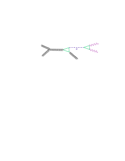
In addition to the QCD contributions discussed above one has to include also electroweak ones. Some examples are shown in Fig.3.
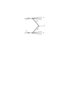

Some examples of electoweak corrections with exchange of bosons
The corresponding proton-proton cross section can be written as
| (4) |
3 Results
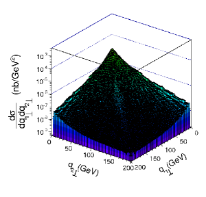
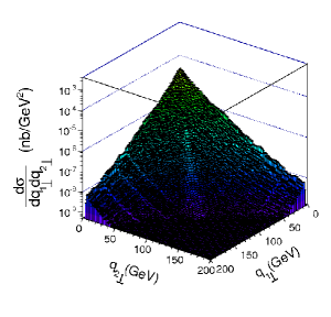
The different UGDFs in the literature have quite different dependence on gluon transverse momenta. In Fig. 4 we show an example of two-dimensional maps in (transverse momenta of the fusing gluons) for two UGDFs. Many more examples were presented in [12]. In Ref.[12] we concluded that a use of saturation inspired scale independent UGDFs is not sufficient for the Higgs boson production. They lead also to distributions in and which are peaked in extremely small and , at least for the leading order subprocess. Quite large gluon transverse momenta () enter the production of the Higgs boson for the KMR and Jung CCFM (set) UGDFs. For the KMR UGDF a clear enhancement at small or can be observed. This is rather a region of nonperturbative nature, where the KMR UGDF is rather extrapolated than calculated. We have checked, however, that the contribution of the region when 2 GeV or 2 GeV constitutes only less than of the integrated cross section. This is then a simple estimate of uncertainty of the whole approach.
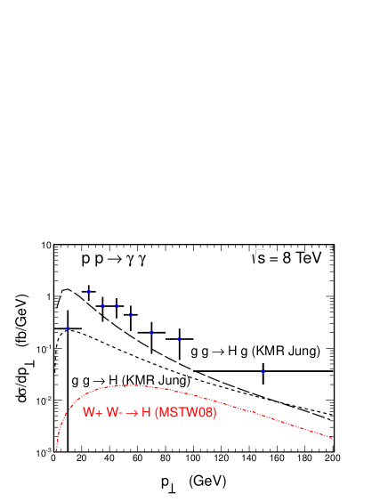
A distribution in Higgs boson transverse momentum is particularly interesting. In Fig. 5 we compare contributions of different mechanisms. The QCD contributions shown in this subsection were calculated with the KMR UGDF. Surprisingly the contribution of the next-to-leading order mechanism is even slightly bigger than that for the fusion, especially for intermediate Higgs boson transverse momenta. As discussed in our original paper [12] there is almost no double counting when adding the corresponding cross sections due to quite different topology of corresponding Feynman diagrams. As shown in the present analysis the mechanism is not sufficient within the -factorization approach. The contribution of the subprocess is also not negligible but here one can expect that a big part is already contained in the calculation especially with the KMR UGDF. Therefore we do not add this contribution explicitly when calculating . The contribution of the , fusion is also fairly sizeable. In principle, the Higgs bosons (or photons from the Higgs boson) associated with the electroweak boson exchanges could be to some extend separated by requiring rapidity gaps i.e. production of Higgs boson isolated off other hadronic activity.
4 Conclusions
We have presented results of our analysis of production of Higgs boson in the two-photon channel within -factorization. Matrix elements and UGDFs are the ingredients of the approach.
We have found that different UGDFs (not discussed here) give quite different results. However, many of the UGDF models were adjusted to low-x phenomena and cannot be used for production of relatively heavy Higgs boson, where rather large gluon transverse momenta are involved.
LO -factorization underpredicts the two-photon data in contrast to recent claims. NLO corrections have to be taken into account and the subprocess is especially important. Also a contribution of Higgs boson associated with quark/antiquark dijets is nonnegligible [12]. Electroweak corrections (here only fusion was discusssed) were found to be large at large transverse momenta of the Higgs boson.
Only combined analysis including all ingredients can provide a possibility to describe experimental data and to test UGDFs. We expect that future run2 data will allow for better tests of UGDFs.
References
-
[1]
G. Aad et al. (the ATLAS Collaboration), Phys. Lett. B716, 1 (2012);
S. Chatrchyan et al. (the CMS Collaboration), Phys. Lett. B716, 30 (2012). - [2] G. Aad et al. (the ATLAS Collaboration), Phys. Lett. B726, 88 (2013); corrigendum: Phys. Lett. B734, 406 (2014).
- [3] S. Chatrchyan et al. (the CMS Collaboration), Phys. Rev. D89, 092007 (2014).
- [4] V. Khachatryan et al. (the CMS Collaboration), arXiv:1405.3455 [hep-ex].
- [5] G. Aad et al. (the ATLAS Collaboration), arXiv:1406.3827 [hep-ex].
-
[6]
R.V. Harlander and W.B. Kilgore,
Phys. Rev. Lett. 88 (2002) 201801;
C. Anastasiou and K. Melnikov, Nucl. Phys. B646 (2002) 220;
V. Ravindran, J. Smith and W.L. van Neerven, Nucl. Phys. B665 (2003) 325. - [7] P. Cipriano, S. Dooling, A. Grebenyuk, P. Gunnellini, F. Hautmann, H. Jung and P. Katsas, Phys. Rev. D88 (2013) 097501.
- [8] A.V. Lipatov, M.A. Malyshev and N.P. Zotov, Phys. Lett. B735, 79 (2014); arXiv:1402.6481 [hep-ph].
-
[9]
M.A. Kimber, A.D. Martin and M.G. Ryskin, Phys. Rev. D63 (2001) 114027;
G. Watt, A.D. Martin and M.G. Ryskin, Eur. Phys. J. C31 (2003) 73. -
[10]
H. Jung, G.P. Salam, Eur. Phys. J. C19 (2001) 351;
H. Jung, arXiv:0411287 [hep-ph]. - [11] ATLAS collaboration, ATLAS note, ATLAS-CONF-2013-072.
- [12] A. Szczurek, M. Luszczak and R. Maciula, Phys. Rev. D90 (2014) 094023.