Lipschitz Changes of Variables between
Perturbations of Log-concave Measures
Abstract.
Extending a result of Caffarelli, we provide global Lipschitz changes of variables between compactly supported perturbations of log-concave measures.
The result is based on a combination of ideas from optimal transportation theory and a new Pogorelov-type estimate. In the case of radially symmetric measures, Lipschitz changes of variables are obtained for a much broader class of perturbations.
Mathematics Subject Classification: 49Q20, 35J96, 26D10
1. Introduction
In [4], Caffarelli built Lipschitz changes of variables between log-concave probability measures. More precisely, he showed that if are convex functions with and for a.e. with , then there exists a Lipschitz map such that 111Given two finite Borel measures and and a Borel map , recall that if and
| (1.1) |
The map is obtained via optimal transportation. It is the unique solution of the Monge problem for quadratic cost:
(see Section 2 for more details, and [12] for a completely different construction of a Lipschitz change of variables in this setting). We note that a particularly important feature of Caffarelli’s result is that the bound (1.1) is independent of the dimension .
A consequence of Caffarelli’s result is the possible deduction of certain functional inequalities (such as log-Sobolev or Poincaré-type inequalities) for log-concave measures from their corresponding Gaussian versions. For instance, denoting the standard Gaussian measure on by , consider the Gaussian log-Sobolev inequality,
which holds for every function . For any measure such that there exists a Lipschitz change of variables between and the Gaussian measure, namely , we deduce, applying the change of variable formula twice, that
Therefore, enjoys a log-Sobolev inequality with constant .
Besides the natural consequences described in [4] and above, Caffarelli’s Theorem has found numerous applications in various fields: indeed, it can be used to transfer isoperimetric inequalities, to obtain correlation inequalities, and more (see, for instance,
[6, 7, 11, 13]).
In this paper, we extend the result of Caffarelli by building Lipschitz changes of variables between perturbations of and that are not necessarily convex. Perturbations of log-concave measures (in particular, perturbations of Gaussian measures) appear, for instance, in quantum physics as a means to help understanding solutions to physical theories with nonlinear equations of motion. In cases where an explicit solution is unknown, perturbations of log-concave measures can be used to yield approximate solutions.
We let denote the space of probability measures on a metric space . The main result of the paper is the following:
Theorem 1.1.
Let be such that . Suppose that and there exist constants for which for a.e. . Moreover, let , , and be such that . Assume that in the sense of distributions for some constant . Then, there exists a constant , independent of , such that the optimal transport map that takes to satisfies
| (1.2) |
The crucial point here is that the estimate on the Lipschitz constant of the optimal transport map is independent of dimension, as it is in Caffarelli’s results for log-concave measures.
In the case of spherically symmetric measures, we are able to weaken the assumptions on both the log-concave measure and its perturbation and still obtain a global Lipschitz change of variables. In particular, the Lipschitz constant is controlled only by the -norm of the positive and negative parts of the perturbation , denoted by and . In the following theorem, we first analyze the -dimensional problem:
Theorem 1.2.
Let be a convex function and be a bounded function such that . Then, the optimal transport that takes to is Lipschitz and satisfies
| (1.3) |
We remark that while the map in Theorem 1.2 is only unique up to sets of -measure zero, arguing by approximation, we can find a particular transport for which the estimate on in (1.3) is satisfied almost everywhere in . Applying this -dimensional result to radially symmetric densities, we obtain the following:
Theorem 1.3.
Let be a convex, radially symmetric function and be a bounded, radially symmetric function such that . Then, the optimal transport that takes to is Lipschitz and satisfies
| (1.4) |
Note that the assumption in Theorems 1.2 and 1.3, unlike in Theorem 1.1, is nonrestrictive. Since is not required to be compactly supported, the normalization constant making a probability measure if it were not already can simply be absorbed into .
We further remark that the -dimensional estimate in Theorem 1.2 is false in higher dimensions when one does not assume that the densities are radially symmetric. More precisely, taking the reference measure to be the standard Gaussian measure, the estimate
| (1.5) |
cannot be true for (see Remark 5.2 to understand the relationship between (1.3) and (1.5) for ). This is manifest if we recall that the Monge-Ampère equation linearizes to the Poisson equation, which does not enjoy estimates for bounded right-hand side. In other words, given and to be chosen, letting be the potential such that takes to (for simplicity, we omit the normalization constant that makes a probability measure) and setting , we have that
for every . The estimate (1.5) implies that and, therefore, the existence of a solution to the Poisson equation with bounded right-hand side, an impossibility in higher dimensions.
Although this heuristic argument is convincing, the details of the proof are rather delicate, and we give them in the Appendix for completeness.
Acknowledgments. M. Colombo acknowledges the support of the Gruppo Nazionale per l’Analisi Matematica, la Probabilità e le loro Applicazioni (GNAMPA) of the Istituto Nazionale di Alta Matematica (INdAM). A. Figalli has been partially supported by NSF Grant DMS-1262411 and NSF Grant DMS-1361122. Y. Jhaveri would like to thank Pablo Stinga for helpful conversations. Part of this work was done while the authors were guests of the FIM at ETH Zürich in the Fall of 2014; the hospitality of the Institute is gratefully acknowledged.
2. Preliminaries
We begin with some preliminaries on optimal transportation and the Monge-Ampère equation, and we fix some notation.
Let . The Monge optimal transport problem for quadratic cost consists of finding the most efficient way to take to given that the transportation cost to move from a point to a point is . Hence, one is led to minimize
among all maps such that . A relaxed formulation of Monge’s problem, due to Kantorovich, is to minimize
among all transport plans , namely the measures whose marginals are and . By a classical theorem of Brenier [2], the existence and uniqueness of an optimal transport plan are guaranteed when is absolutely continuous and and have finite second moments. Additionally, the optimality of a transport plan is equivalent to where is a convex function, often called the potential associated to the optimal transport. As a consequence, it follows that in the Monge problem, unique optimal maps exist as gradients of convex functions.
Theorem 2.1.
Let such that and
Then, there exists a unique (up to sets of -measure zero) optimal transport taking to . Moreover, there is a convex function such that .
A direct consequence of Brenier’s characterization of optimal transports as gradients of convex functions is that
| (2.1) |
which follows immediately from the monotonicity of gradients of convex functions.
Suppose now that and , and let be a convex function such that for the optimal transport that takes to . Assuming that is a smooth diffeomorphism, the standard change of variables formula implies that
Hence, assuming that , we see that is a solution to the Monge-Ampère equation
This formal link between optimal transportation and Monge-Ampère (since, to deduce the above equation, we assumed that was already smooth) is at the heart of the regularity of optimal transport maps (see, for instance, [8] for more details). In particular, Caffarelli showed the following in [3] (see also [9, Theorem 4.5.2]):
Theorem 2.2.
Let be bounded open sets, and and be probability densities locally bounded away from zero and infinity. If is convex, then for any set , the optimal transport between and is of class for some . In addition, if and for some and , then .
As mentioned in [1], Caffarelli’s regularity result on optimal transports can be extended to the case where and are defined on all of and assumed to be locally bounded away from zero and infinity. Lastly, we note that optimal transport maps are stable under approximation (see [15]). In particular, let and be locally uniformly bounded probability densities such that and in . Then, the associated potentials locally uniformly and in measure.
We fix the following additional notation:
3. Lipschitz Changes of Variables between Log-concave Measures
We begin with two useful results of Caffarelli (see [4]). They provide some motivation, and we briefly recall their proofs both for completeness and because we shall need them later.
Lemma 3.1.
Let with finite second moments and be the optimal transport taking to . Assume that and that is bounded away from zero in the ball for some and vanishes outside . Then,
In particular, for any fixed and for all , the function as .
Proof.
We begin by noticing that, as a consequence of Theorem 2.2, is continuous on and, in particular, the map is well defined at every point.
Let and be fixed, and consider the cone with vertex at and pointing in the -direction
By (2.1) we see that
hence
and so, up to a set of measure zero, the preimage of under is contained in the (concave) cone
Moreover, since ,
Let , and notice that . This proves that .
Now, as since covers as . Recalling that is bounded away from zero in , we have that
Letting , we see that . As the point was fixed arbitrarily, uniformly as . Thus, behaves like the cone at infinity. In particular, for any fixed and for all , the function as . ∎
Theorem 3.2.
Let be such that . Suppose there exist constants such that and for a.e. . Then, the optimal transport that takes to is globally Lipschitz and satisfies
| (3.1) |
Proof.
By the stability of optimal transports, we may assume that is equal to infinity outside the ball for some fixed . Indeed, define
and such that
Clearly, in as . Hence, if we prove (3.1) for the optimal transport that takes to , letting we obtain the same estimate for .
Also, by Theorem 2.2, the convex potential associated to the optimal transport is of class ; therefore, satisfies the Monge-Ampère equation
or equivalently,
| (3.2) |
For fixed , we define the incremental quotient of a function at by
By convexity of we see that . Also, it follows by Lemma 3.1 that as . Thus attains a global maximum at some . Up to a rotation, we assume that . Thus,
| (3.3) |
Moreover, because is the maximal direction,
Taking for and utilizing (3.3), we see that all the components but the first of , , and are equal. Let , and observe that, by (3.3),
Hence, we conclude that
| (3.4) |
Another consequence of achieving a maximum at is
| (3.5) |
We recall that
| (3.6) |
for all square matrices and with invertible. Also, if we set , since is concave on the space of positive semidefinite matrices and recalling (3.6), we have
and
In particular, from (3.5) and the convexity of , we deduce that
Now, let us, for fixed , consider the incremental quotient of (3.2) at . Using (3.4), we realize that
| (3.7) |
Observe that
hence,
| (3.8) |
Furthermore, from (3.4), we similarly see that
Combining this estimate with (3.8) and (3.7), we get
| (3.9) |
Set . Since
the convexity of , (3.4), and (3.9) give us that
and so
Notice that this is the desired estimate up to a factor . We use a bootstrapping argument to remove this factor. Suppose that for some . For any , by (3.4) and (3.9),
Thus,
In other words, if with , then
Starting with and repeating the above procedure an infinite number of times, we prove (3.1) since uniquely solves . ∎
Remark 3.3.
Notice that the above proof relies only on the local behavior of our densities and . In particular, the bounds on the Hessians of and are only used near the maximum point and its image , respectively. This simple observation will play an important role in the proof of Theorem 1.1.
Remark 3.4.
The above result is not ideal. Indeed, if , then and one would like to have the bound instead of .
4. Compactly Supported Perturbations: Proof of Theorem 1.1
In the following lemma, we prove an upper bound on how far points travel under the transport map when the source measure is perturbed in a certain fixed ball . We capture and quantify that our perturbations are compactly supported. Lemma 4.1 will be applied in the proof of Theorem 1.1 to the inverse transport.
Furthermore, given our convex function , we consider, for ,
| (4.1) |
and we approximate with compactly supported measures . This approximation is in the spirit of Caffarelli’s approximation in the proof of Theorem 3.2. It allows us to find maximum points of a suitable function and guarantees that they do not escape to infinity in the proof of Theorem 1.1. This approximation procedure is purely technical. Hence, on a first reading of Lemma 4.1, the reader may just take .
Lemma 4.1.
Let be such that . Suppose that and there exist constants such that for all . Moreover, let , , and be such that . Given , set as in (4.1) and choose such that . If is the optimal transport map that takes to , then there exist constants and such that for all ,
| (4.2) |
Even though this lemma is not independent of dimension as written (specifically, depends on ), the dimensional dependence does not affect the constant and disappears in the limit as . Thus, we can indeed prove a global estimate on the optimal transport taking to that is independent of dimension.
Lemma 4.1 is written under slightly different assumptions than Theorem 1.1. In particular, besides the obvious additional regularity assumptions on and its perturbation, made only for simplicity, we have not required that the perturbation be semiconvex. That said, if we assume the the distributional Hessian of is indeed bounded below by , then we can replace the dependence on with a dependence on , as explained in the following remark.
Remark 4.2.
Let be a function compactly supported in that satisfies the semiconvexity condition in the sense of distributions. Then, its -norm is controlled by a constant depending only on and (in particular, it is independent of dimension):
| (4.3) |
First, up to convolving with a standard convolution kernel, we can assume that is smooth. Then, we observe that every 1-dimensional restriction , for and , is compactly supported in and has second derivative bounded below by . This implies that
| (4.4) |
Indeed, suppose to the contrary that for some . By integration, we would get
Impossible. This proves (4.4), and (4.3) holds by integrating.
Before proceeding with the proof of Lemma 4.1, we recall a Talagrand-type transport inequality. Given , we denote the squared Wasserstein distance between and by (see [15, Chapter 6] for the general definition), and we consider their relative entropy
Here, is the relative density of with respect to . If for some such that for all , we have that (see [6], applied in the particular case when and are probability measures)
| (4.5) |
In our applications, coincides with the cost of the optimal transport taking to .
Proof of Lemma 4.1.
Notice first that, as a consequence of Theorem 2.2, is continuous.
Assume there exists a point with (otherwise, the statement is true with ). We show that for some that will be chosen later. Let
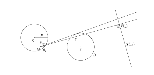
and define the constant and ball by and . Also, let be the projection of a point onto the hyperplane through and perpendicular to . The map is well-defined because (see Figure 4.1). Let us assume that , so that .
By (2.1), we have that
and as is the closest point to in the set },
(see Figure 4.1). Given any , either , , and determine a plane, call it , within which , , and determine a right triangle, or , , and are collinear. Thus,
where is the angle between and . Now, is a circle of radius centered at . Letting be the angle between the line through and tangent to and the line through and , we see that . (While there are two such tangent lines, the angles they determine with the line through and are the same. Again, see Figure 4.1.) Moreover, and . Consequently,
and
Since and , by restricting to -dimensional lines through the origin we have that
| (4.6) |
hence, as ,
We now estimate . Since and , we have
| (4.7) |
Furthermore, we claim that the following upper bound on holds:
| (4.8) |
To see this, first, apply the Talagrand-type transport inequality (4.5) with and to find that
| (4.9) |
Second, choose , so that
Notice that since
| (4.10) |
So, for every , observe that
and then, recalling that , note
| (4.11) |
Now, use Jensen’s inequality on (4.10) and that is supported in to deduce that
| (4.12) |
Finally, combine (4.9), (4.11), and (4.12) to see that (4.8) holds as claimed.
The following result is a Pogorelov-type a priori estimate on pure second derivatives of the potential associated to our optimal transport. This technique is inspired by Pogorelov’s original argument for the classical Monge-Ampère equation [14]. In our case, we face the additional difficulty of constructing an auxiliary function that compensates for the concavity of our perturbation and the growth of our convex function at infinity. Assuming that our auxiliary function attains a finite maximum, we provide a quantitative estimate on the value of at its finite maximum. This result contains and overcomes the primary obstacles to demonstrating that our optimal transport is globally Lipschitz.
Before stating the result, we introduce some constants and an auxiliary function , all depending only on the constants , and that appear in Theorem 1.1. Define the constants and by
| (4.14) |
let be given by
| (4.15) |
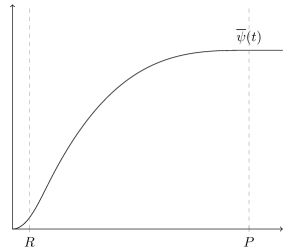
and let be defined by
| (4.16) |
Observe that the function is defined in such a way that in , on , and is supported in (see Figure 4.2).
Proposition 4.3.
Let , and be defined as in Theorem 1.1. Assume, additionally, that and are smooth. Let , and be defined as in (4.14), (4.15), and (4.16). Given , set as in (4.1) and choose such that . Also, let solve
and assume that there exist constants such that for all ,
| (4.17) |
or equivalently, that . If
| (4.18) |
attains a maximum at some point among all possible , then there exists a constant , yet independent of , such that
Proof.
Since, by assumption, is a maximum point of , we have . This implies that is an eigenvector of . Therefore, up to a rotation, we assume that and that is diagonal at . Throughout this proof, the function is seen as a function of the variable with fixed. Then, at we compute that
| (4.19) |
for all , and
| (4.20) |
where we denote the inverse matrix of by .
Let . Using (3.6), we differentiate the equation
| (4.21) |
in the -direction twice to obtain
and
| (4.22) |
By (4.20) and (4.22), we deduce that at
| (4.23) | ||||
We estimate each term in (4.23) from below. Recall that and are diagonal at . Therefore, , and we see that
and
Because has a maximum at among all directions,
| (4.24) |
and so
Additionally, differentiating (4.21) in the -direction, we have that
By (4.19), it then follows that
and, consequently, (4.23) becomes
| (4.25) |
If , (4.17) implies that . Then, since the gradient of is zero outside by construction. If, on the other hand, , then
(Here, we have used that and that to show is bounded above by .) In both cases, we deduce that
for a constant depending only on , , , , and . Thus, by (4.25), we have that
| (4.26) |
We claim that
| (4.27) |
Indeed, let us consider two cases, according to whether or not belongs to . If , then
and (4.27) follows. In the case that , we compute the derivatives of in terms of the derivatives of . Observe that
Thus,
since in and . Then, (4.24) implies that
| (4.28) |
As , we know . It follows that
| (4.29) |
By (4.28) and (4.29), we deduce that (4.27) holds in this case as well.
Notice that if , then . In this case, the constant found in the proof above is zero, and we recover the global Lipschitz constant obtained by Caffarelli in Theorem 3.2 up to a factor of (this is a better bound than the one provided by the proof of Theorem 3.2 before the final bootstrapping argument).
Proof of Theorem 1.1.
We first prove the statement assuming that and are smooth. For every set as in (4.1), and choose such that . Let be the optimal transport map that takes to . Since the density is supported in a convex set, smooth on its support, and is bounded from above and below by positive constants, by Theorem 2.2, we deduce that . By the stability of optimal transport maps, it suffices to show that for all ( to be chosen possibly depending on ) we have that
| (4.31) |
for some constant depending only on , , , and .
Let , and be defined as in (4.14), (4.16), and (4.18). Applying Lemma 4.1 to the optimal transport , we see that there exist constants and (see Remark 4.2) such that for all ; that is, letting (for simplicity we omit in the dependence on , which can be any number greater than in the following),
| (4.32) |
We split the proof in two cases, according whether or not achieves a maximum in . If there exists such that
then we apply Proposition 4.3 and see that
which proves (4.31).
Otherwise, we consider the maxima of in with . Let
Notice that is nondecreasing (and not definitively constant) and as . Now, consider the functions approximating defined by
Since is smooth, we know that locally uniformly in as . Furthermore, by Lemma 3.1,
| (4.33) |
uniformly with respect to and . Since (by the convexity of ), the function has a finite maximum point .
We claim that for sufficiently small (possibly depending on and on the sequence )
| (4.34) |
Indeed, let and be such that and . Since converges to locally uniformly, there exists such that
for every , , and . So, for every , we have that
| (4.35) |
Thus,
| (4.36) |
for every , , and . Since , (4.35) and (4.36) imply that in . Therefore, satisfies (4.34) for every .
Recall that is constant outside . Then, by (4.32) and (4.34), we know that for every , the function is locally constant around . Therefore, is also a local maximum point for the incremental quotient . Moreover, outside the function is convex as it coincides with . So, proceeding as in the proof of Theorem 3.2 (cf. Remark 3.3), we conclude that (4.31) is also proved in the case that is not guaranteed to achieve a maximum in .
In order to remove the smoothness assumptions on and , we approximate and by convolution (adding a small constant to ensure these approximations define probability measures). Then, from what we have shown above, the approximate transports are all globally and uniformly Lipschitz. Thanks to the stability of optimal transports, passing to the limit, we prove (1.2). ∎
5. Bounded Perturbations in -Dimension and in the Radially Symmetric Case: Proofs of Theorems 1.2 and 1.3
Our goal now is to produce optimal global Lipschitz estimates under strong symmetry but weak regularity assumptions on our log-concave measures. Notice that when our perturbation is zero, we recover that our optimal transport is the identity map (cf. Remark 3.4). We begin in -dimension and with a technical lemma relating the behavior of our convex base and the cumulative distribution function of the log-concave probability measure it defines.
Lemma 5.1.
Let be a convex function such that and be such that . Define , by
| (5.1) |
Then,
| (5.2) |
and
| (5.3) |
Proof.
Since an analogous argument proves (5.3), we only show (5.2); in other words, we prove that the function is nondecreasing in . Let . The function is clearly nondecreasing in , whenever this interval is not a single point. Moreover, it is locally Lipschitz and its derivative is . Hence, it suffices to show that the derivative is nonnegative in . Since is nonincreasing in and by the change of variables formula, we have that for a.e.
which proves our claim. ∎
Proof of Theorem 1.2.
By approximating with a sequence of convex functions such that and that are finite on , we can assume that on . This reduction follows from the stability of optimal transport maps. Recall that, as a consequence of the push-forward condition , satisfies the mass balance equation
| (5.4) |
which can be also written as
| (5.5) |
since the measures and have total mass . From (5.4), we deduce that is differentiable. Indeed, both the functions
are differentiable and their derivatives do not vanish. So, is differentiable as well. Thus, differentiating with respect to and then taking the logarithm shows that
Consequently,
| (5.6) |
On the other hand, (5.4) implies that
since . Taking the logarithm and defining as in (5.1), we see that
| (5.7) |
Analogously, from (5.5), we deduce that
| (5.8) |
We claim that
| (5.9) |
To prove this claim, let be such that and consider the sets
Applying (5.2) in yields that
if and
whenever . Therefore, (5.9) holds in by (5.7). Similarly, applying (5.3) gives us that (5.9) holds in by (5.8). Now, we consider three cases:
1. If , the monotonicity of implies that , and (5.9) holds in all of .
2. If , then where, thanks to the monotonicity of , we have
Since attains its minimum at , is decreasing on and increasing on . Consequently,
As and , our above analysis shows that (5.9) holds in .
3. If , an analogous argument to one used to prove case 2 demonstrates that where and proves (5.9) also in .
Remark 5.2.
From the numerical inequality , which holds for , we see that if is the potential associated to in Theorem 1.2, then provided that , there exists a constant such that
We now move to the radially symmetric case in -dimensions.
Proof of Theorem 1.3.
Let be two functions such that on , and and for every . Now, consider the function
where is the optimal transport that takes to .
Set . We first claim that the optimal transport is Lipschitz and satisfies
| (5.10) |
Indeed, let be defined by on and infinity otherwise, and let on and zero elsewhere. Observe that is convex and is bounded. Hence, applying Proposition 1.2 with and proves (5.10).
We now conclude the proof. Notice that is continuous. Furthermore, is an admissible change of variables from to . To see this, we show that for every bounded, Borel function ,
| (5.11) |
The formula (5.11) can be rewritten, using polar coordinates and the definition of , as
which is, in turn, satisfied if we use the test function and recall the definition of .
Now, let and . Since , we observe that
where . By (5.10), we deduce that
which proves (1.4). To conclude, we show that is the optimal transport taking to . Let be the convex potential associated to . By construction, and is a convex function. Since optimal transports are characterized by being gradients of convex functions, is the optimal transport taking to . ∎
6. Appendix
We now show that the linear bound in Remark 5.2 is specific to the -dimensional case.
Proposition 6.1.
Let and , so that is the standard Gaussian density in . Then, for every , there exists a bounded, continuous perturbation such that and and the optimal transport that takes to satisfies
Proof.
Suppose, to the contrary, that for every bounded, continuous function with , the optimal transport that takes to satisfies
| (6.1) |
for some . In particular, let , and for all , define by
By construction, . Thus, let be the potential associated to the optimal transport that takes to , and remember that solves the Monge-Ampère equation
| (6.2) |
Note that as . Also, since
is Lipschitz as a function of and
| (6.3) |
In addition, by the dominated convergence theorem,
| (6.4) |
Without loss of generality, we assume that . Now, define
By (6.1) applied to and (6.3), we see that if , then
| (6.5) |
Recall that, for any matrix , there exists a , depending only on , such that for all sufficiently small . Therefore, there exist an and a collection of functions with
| (6.6) |
such that for all ,
Thus, by (6.2) and our choice of ,
| (6.7) |
We claim that, up to a subsequence, there exists a function such that in and weakly- in as . To this end, by Arzelà-Ascoli, it suffices to show that are locally bounded in . Since , by (6.5), it is enough to prove that
| (6.8) |
Assume, to the contrary, that . Notice that (6.7) implies that for all and ,
Let , and note that up to subsequences as . Furthermore, let be a nonnegative function that integrates to one. Then, by (6.3), we deduce that
| (6.9) |
Recall that converges uniformly to the identity matrix by (6.1) applied to and . By the stability and uniqueness of optimal transports, converges locally uniformly to the identity map as . In particular, for every and sufficiently small, and we obtain that
by dominated convergence. Thus, taking the limit in (6.9) and noticing that the right-hand side is bounded as thanks to (6.5) and (6.6), we see that
which, being impossible, proves (6.8) and shows that in and weakly- in as for some function .
Now, reformulating (6.7), we see that for any ,
| (6.10) |
Thus, recalling (6.4) and that is continuous, we can pass to the limit and obtain that
for all . Since was arbitrary, we have shown that for every , there exists a function solution to
| (6.11) |
We now show that this is impossible. Recall that there exists a bounded, continuous and , for any , such that in , yet . In particular, . (See [10, Chapter 3].) Define
and observe that, since and is bounded and continuous, . By construction, there exists a that solves (6.11) with . Then, for we have that in . Thus, by elliptic regularity, a contradiction since and . ∎
References
- [1] S. Alesker, S. Dar, and V. Milman, A remarkable measure preserving diffeomorphism between two convex bodies in , Geom. Dedicata 74(2) (1999), 201-212.
- [2] Y. Brenier, Polar factorization and monotone rearrangement of vector-valued functions, Comm. Pure Appl. Math. 44(4) (1991), 365-417.
- [3] L. A. Caffarelli, The regularity of mappings with a convex potential, J. Amer. Math. Soc. 5(1) (1992), 99-104.
- [4] L. A. Caffarelli, Monotonicity properties of optimal transportation and the FKG and related inequalities, Comm. Math. Phys. 214(3) (2000), 547-563.
- [5] L. A. Caffarelli, Erratum: Monotonicity properties of optimal transportation and the FKG and related inequalities, Comm. Math. Phys. 225(2) (2002), 449-450.
- [6] D. Cordero-Erausquin, Some applications of mass transport to Gaussian-type inequalities, Arch. Rat. Mech. Anal. 161(3) (2002), 257-269.
- [7] D. Cordero-Erausquin, M. Fradelizi, and B. Maurey, The (B) conjecture for the Gaussian measure of dilates of symmetric convex sets and related problems, J. Funct. Anal. 214(2) (2004), 410-427.
- [8] G. De Philippis and A. Figalli, The Monge-Ampère equation and its link to optimal transportation, Bull. Amer. Math. Soc. (N.S.) 51(4) (2014), 527-580.
- [9] A. Figalli, ”The Monge-Ampère Equation and its Applications”, Zürich Lectures in Advanced Mathematics, to appear.
- [10] Q. Han and F. Lin, ”Elliptic Partial Differential Equations”, 2nd Edition, Courant Lecture Notes in Mathematics, Vol. 1, New York University, Courant Institute of Mathematical Sciences, New York, American Mathematical Society, Providence, 1997.
- [11] G. Hargé, A convex/log-concave correlation inequality for Gaussian measure and an application to abstract Wiener spaces, Probab. Theory Related Fields 130(3) (2004), 415-440.
- [12] Y.-H. Kim and E. Milman, A generalization of Caffarelli’s contraction theorem via (reverse) heat flow, Math. Ann. 354(3) (2012), 827-862.
- [13] B. Klartag, Marginals of geometric inequalities, In: ”Geometric Aspects of Functional Analysis”, V. D. Milman and G. Schechtman (eds.), Lecture Notes in Mathematics, Vol. 1910, Springer Berlin, 2007, 133-166.
- [14] A. V. Pogorelov, The regularity of generalized solutions of the equation , (Russian) Dokl. Akad. Nauk SSSR 200 (1971), 534-537.
- [15] C. Villani, ”Optimal Transport, Old and New”, Grundlehren des mathematischen Wissenschaften [Fundamental Principles of Mathematical Sciences], Vol. 338, Springer-Verlag Berlin Heidelberg, 2009.