Hermitian codes and complete intersections

Abstract.

In this paper we consider the Hermitian codes defined as the dual codes of one-point evaluation codes on the Hermitian curve $\mathcal{H}$ over the finite field $\mathbb{F}_{q^{2}}$. We focus on those with distance $d\geq q^{2}-q$ and give a geometric description of the support of their minimum-weight codewords.
We consider the unique writing $\mu q+\lambda(q+1)$ of the distance $d$ with $\mu,\lambda$ non negative integers, and $\mu\leq q$, and consider all the curves $\mathcal{X}$ of the affine plane $\mathbb{A}^{2}_{\mathbb{F}_{q^{2}}}$ of degree $\mu+\lambda$ defined by polynomials with $x^{\mu}y^{\lambda}$ as leading monomial w.r.t. the DegRevLex term ordering (with $y>x$). We prove that a zero-dimensional subscheme $Z$ of $\mathbb{A}^{2}_{\mathbb{F}_{q^{2}}}$ is the support of a minimum-weight codeword of the Hermitian code with distance $d$ if and only if it is made of $d$ simple $\mathbb{F}_{q^{2}}$-points and there is a curve $\mathcal{X}$ such that $Z$ coincides with the scheme theoretic intersection $\mathcal{H}\cap\mathcal{X}$ (namely, as a cycle, $Z=\mathcal{H}\cdot\mathcal{X}$). Finally, exploiting this geometric characterization, we propose an algorithm to compute the number of minimum weight codewords and we present comparison tables between our algorithm and MAGMA command MinimumWords.

1. Introduction

Let $q$ be a power of a prime. The Hermitian curve $\mathcal{H}$ is the affine, plane curve defined by the polynomial $x^{q+1}=y^{q}+y$. It is a smooth curve of genus $g=\frac{q^{2}-q}{2}$ with only one point at infinity. The curve $\mathcal{H}$ is one of the best known example of maximal curve, that is with the maximum number of $\mathbb{F}_{q^{2}}$-points allowed by the Hasse-Weil bound [32].

Starting from the Hermitian curve and any positive integer $m$, it is possible to construct the geometric one-point Goppa code $C_{m}$ on $\mathcal{H}$, that is called Hermitian code. This is by far the most studied among geometric Goppa codes, due to the good properties of the Hermitian curve.

For a thorough exposition of the main features of Hermitian curves and codes we refer to [12] and to Section 8.3 of [35].

In 1988, Stichtenoth [34] describe generator and parity-check matrices of Hermitian codes, introduced one year before by van Lint, Springer [23] and Tiersma [36]. Stichtenoth, for any $m>q^{2}-q-2$, finds a formula for the distance $d$ of $C_{m}$. A few years later, Yang and Kumar [37] bring to completion Stichtenoth work finding the distance of the remaining codes $C_{m}$. Finally, in 1995 Kirfel and Pellikaan [19] presented a different and much shorter proof of these results using linear algebra and the theory of semigroups. Since then, the results were extended to two-point Hermitian codes by Homma and Kim [14, 15, 16, 17] exploiting a similar proof to [37]. After that, in 2010 Park [30], using a method based on [19], gives a short and easy proof of the same results of Homma and Kim and obtains a geometrical characterization of minimum weight codewords as multiplications of conics and lines. The description of minimum-weight codewords of some two-points Hermitian codes have been found three years later by Ballico and Ravagnani [2] using different techniques. Moreover, Yang [38] and Munuera [28] obtain the values of many generalized Hamming weights also called weight hierarchies. Finally, Barbero and Munera [4] find the complete sequence of weight hierarchies of Hermitian codes by an exhaustive computation of the bounds given by Heijnen and Pellikaan [11]. Other results concerning generalized Hamming weights of codes on Hermitian curve and the relative generalized Hamming weights can be found i.e. in [1, 9, 18, 20].

In [13] the Hermitian codes are seen as a sub-family of evaluation codes. Using this different approach, the authors divide the codes $C_{m}$ in four phases with respect to the integer $m$, and for each of them give explicit formulas linking dimension and distance. In this paper we adopt their classification of Hermitian codes in four phases (with minor changes, as summarized in Table 1) and, as in [13], we consider the Hermitian code as the dual of one-point evaluation code (Definition 2.8).

Later on, the research about Hermitian codes branches out in several different lines. Some papers, as for instance [21, 22, 25, 29], deal with the problem of finding efficient algorithms for the decoding of the Hermitian codes.

An hard problem is that of determining the weight distribution, in particular the small-weight distribution. So far, few partial results are known, and the first of them appears only in 2011 ([31]).
The geometric characterization of the small-weight codewords of the Hermitian code $C_{m}$ for a few cases of $m$ (mainly in the first and second phase) can be found in [3, 5, 6, 26, 31]. In particular in [31] and [26], the first author of this paper and her co-authors study Hermitian codes $C_{m}$ with distance $d\leq q$, that is with $m\leq q^{2}-2$ (first phase). They prove that the points of the support of any minimum-weight codeword of $C_{m}$ lie in the intersection between a line and $\mathcal{H}$; on the other hand, any set of $d$ points in such a complete intersection corresponds to minimum-weight codewords. This characterization allows the authors to compute the number of minimum-weight codewords.

In 2012, Couvreur [5] investigate the minimum-weight codewords problem for codes over an affine-variety $\mathcal{X}$ by a new method. Quoting Couvreur paper the approach is based on problems á la Cayley-Bacharach and consists in describing the minimal configurations of points on $\mathcal{X}$ which fail to impose independent conditions on forms of some degree.

As an application of this approach, in [6] the authors find a geometric characterization of small-weight codewords of $C_{m}$ for some $m$ and $d\leq 3q-6$ (first and second phase). In particular they prove that the set of points that are the support of a minimum-weight codeword (or a subset of them) is a cut on $\mathcal{H}$ by either a line, or a conic, or the complete intersection of two curves of degrees $q-2$ and $3$. A similar result is found for all codewords of the first phase having weight $v\leq 2d-3$.

A new proof of the above results and some new information about the small-weight codewords of Hermitian codes $C_{m}$ with $m\leq q^{2}+q$ and $d=2q+2,2q+1,2q$ or $d\leq q$ are presented in [3].

So, up to now, the geometric descriptions of minimum weight codewords that we can find in literature concern only a few Hermitian codes, mainly those in the first and second phases (namely, with $m\leq 2q^{2}-2q-3$): note that, for each value of $q$, these two phases cover only a small fraction (about $\frac{2}{q}$) of all the Hermitian codes.

In this paper we provide a geometric characterization for minimum-weight codewords of all the Hermitian codes $C_{m}$ in the remaining two phases. Our main result is the following theorem.

Theorem (Theorem 5.1).

Let $C_{m}$ be an Hermitian code with $m\geq 2q^{2}-2q-2$ and distance $d=m-q^{2}+q+2$. Let $\lambda,\mu$ be the unique pair of non-negative integers such that $d=\mu q+\lambda(q+1)$ and $\mu\leq q$ and let $D$ be a divisor on the Hermitian curve $\mathcal{H}$ made of simple points with coordinates in $\mathbb{F}_{q^{2}}$.
Then $D$ is the support of a minimum-weight codeword of $C_{m}$ if and only if it is the complete intersection of $\mathcal{H}$ and a curve $\mathcal{X}$ defined by a polynomial $F$ of the following type:

(1.1) $$F=x^{\mu}y^{\lambda}+\Sigma a_{i}x^{r_{i}}y^{s_{i}}\hbox{ where either }r_{i}+s_{i}<\mu+\lambda\hbox{ or }r_{i}+s_{i}=\mu+\lambda\hbox{ and }r_{i}<\mu.$$

Besides the theoretical interest of this geometric description, we note that all the properties that are involved can be easily checked through standard tools of computational algebra, as for instance those concerning the ideal membership. In fact we can reformulate the above Theorem as follows (Corollary 5.3)

A zero-dimensional subscheme $D$ of $\mathcal{H}$ is the support of a minimum-weight codeword of $C_{m}$ if and only if the ideal $I_{D}$ of $D$ is generated by $H$ and a polynomial $F$ as in (1.1) and it contains $x^{q^{2}}-x$ and $y^{q^{2}}-y$.

Exploiting this explicit characterization, we propose Algorithm 1 to compute the number of minimum weight codewords. We implemented this algorithm with MAGMA software and we compare its performance with those of the command MinimumWords already present in MAGMA for some codes of the third and fourth phase (i.e. Hermitian codes with $m\geq 2q^{2}-2q-2$) with $q=3$ and $q=4$. Depending on the code the two algorithm have different performances, in general our algorithm is more convenient for lower $m$ (see Table 2). A striking case is that with $q=4$ and $m=22$: our algorithm computes the number of minimum-weight codewords in $85.87$ seconds (they are $150000$), while MinimumWords declares that termination requires $10^{8}$ years.

To achieve these results we use a different term ordering with respect to what can be usually found in literature, that is the $\mathtt{DegRevLex}$ with $y>x$. We exploit tools such as the Hilbert polynomial and the so called sous-éscalier. This last tool, together with Gröbner basis, has already been exploited in a slightly different way in [7, 8, 10] to establish or to determine some affine-variety code parameters.

We also point out that analogous results for codes of the other phases, namely codes $C_{m}$ with $m<2q^{2}-2q-2$, has been obtained by the authors in [27]. Finally, a generalization to codewords of small weight is in progress and we are confident that, from this strong geometric characterization, also the explicit computation of the weight distribution will follow.

The paper is organized as follows:

• In Section 2 we recall some basic definitions about Hermitian curves and codes and we discuss our non-standard choice of the term ordering.

• In Section 3 we focus on the Hermitian codes $C_{m}$ with $m\geq q^{2}-1$ and prove some preliminary results that we will exploit in the following sections.

• In Section 4 we study the Hermitian codes $C_{m}$ with $m\geq 2q^{2}-2q-2$. The main result of this section is Theorem 4.2 which will be key tools in the final section. In some sense it generalize the classical results by Stichtenoth [34] about the distance formula. Indeed, in Corollary 4.3 we recover this same formula as a special case of what is proved in Theorem 4.2.

• In Section 5 we state and prove Theorem 5.1, which gives a geometric characterization for any minimum-weight codewords of the Hermitian codes $C_{m}$ with $m\geq 2q^{2}-2q-2$.

• In Section 6 we propose Algorithm 1 to compute the number of minimum-weight codewords and we present comparison tables (Tables 2,3) with MAGMA command MinimumWords.

• At the end we draw the conclusions.

2. Generalities and introduction to codes

2.1. The geometric setting

Let $\mathbb{F}_{q^{2}}$ be the finite field with $q^{2}$ elements, where $q$ is a power of a prime, and let $K$ be its algebraic closure. For any ideal $I$ in the polynomial ring $\mathbb{F}_{q^{2}}[x,y]$ we denote by $\mathcal{V}(I)$ the corresponding subscheme of $\mathbb{A}_{\mathbb{F}_{q^{2}}}^{2}$; if $g_{1},\ldots,g_{s}\in\mathbb{F}_{q^{2}}[x,y]$, we denote by $\langle g_{1},\ldots,g_{s}\rangle$ the ideal they generate. If $Y$ is a subscheme of $\mathbb{A}_{\mathbb{F}_{q^{2}}}^{2}$, we will denote by $I_{Y}$ the ideal such that $Y=\mathcal{V}(I_{Y})$ and by $A_{Y}$ the coordinate ring of $Y$, namely the quotient $\mathbb{F}_{q^{2}}[x,y]/I_{Y}$.
Though we are mainly interested in the closed points with coordinates in $\mathbb{F}_{q^{2}}$ ($\mathbb{F}_{q^{2}}$-points for short), we will not identify a subscheme of $\mathbb{A}_{\mathbb{F}_{q^{2}}}^{2}$ with the set of its $\mathbb{F}_{q^{2}}$-points, or, more generally, a scheme with its support. For the sake of simplicity, we sometimes consider the reduced schemes as the set of their irreducible components; for instance a zero-dimensional and reduced scheme $Z$, can be considered as the set of its (closed) points and denoted $Z=\{Q_{1},\dots,Q_{s}\}$.

If $Z$ is a zero-dimensional subscheme of $\mathbb{A}_{\mathbb{F}_{q^{2}}}^{2}$, we will say that it is a divisor on a curve $\mathcal{X}$ if $I_{\mathcal{X}}\subset I_{Z}$. Moreover, we will say that $Z$ it is a complete intersection of $\mathcal{X}$ with another curve $\mathcal{Y}$ if $I_{Z}=I_{\mathcal{X}}+I_{\mathcal{Y}}$; in this case we can also write $Z$ as $\sum m_{i}Q_{i}$ where $m_{i}$ is the intersection multiplicity of $\mathcal{X}$ and $\mathcal{Y}$ at $Q_{i}$.

2.2. The Hermitian curve

The Hermitian curve $\mathcal{H}$ is the curve in the affine plane $\mathbb{A}_{\mathbb{F}_{q^{2}}}$ defined by the polynomial $H:=x^{q+1}-y^{q}-y$. We will denote by $I_{\mathcal{H}}$ the ideal in $\mathbb{F}_{q^{2}}[x,y]$ generated by $H$ and by $A_{\mathcal{H}}$ the coordinate ring $\mathbb{F}_{q^{2}}[x,y]/I_{\mathcal{H}}$ of $\mathcal{H}$.

The curve $\mathcal{H}$ has genus $g=\frac{q(q-1)}{2}$ and contains exactly $n:=q^{3}$ $\mathbb{F}_{q^{2}}$-points that we will denote by $P_{1},\dots,P_{n}$ [32]. We will always denote by $E$ the reduced zero-dimensional scheme $\{P_{1},\dots,P_{n}\}$, or, equivalently, the divisor $\Sigma P_{i}$ on $\mathcal{H}$.

The projective closure $\overline{\mathcal{H}}$ of $\mathcal{H}$ in $\mathbb{P}^{2}_{K}$ contains only one more point $P_{\infty}=[0:0:1]$, which is simple and $\mathbb{F}_{q^{2}}$-rational, so that $\overline{\mathcal{H}}$ has $q^{3}+1$ $\mathbb{F}_{q^{2}}$-points.

We recall that the norm $\mathrm{N}$ and the trace $\mathrm{Tr}$ are two functions from $\mathbb{F}_{q^{2}}$ to $\mathbb{F}_{q}$ such that $\mathrm{N}(x)=x^{1+q}\mbox{ and }\mathrm{Tr}(x)=x+x^{q}.$ Observe that $\mathcal{H}=\{\mathrm{N}(x)=\mathrm{Tr}(y)\mid x,y\in\mathbb{F}_{q^{2}}\}$.

Remark 2.1.

In the proof of the key results of this paper we will exploit the beautiful arrangement of the set of $\mathbb{F}_{q^{2}}$-points of the Hermitian curve, due to its norm-trace equation. There are $q^{2}$ vertical lines, each containing $q$ points of $E$, and there are $q^{2}-q+1$ horizontal lines each containing $q+1$ points of $E$. See [CGC-alg-book-hirschfeld1998projective] or Section 2.3 of [26].

Definition 2.2.

An $\mathbb{F}_{q^{2}}$-divisors on the Hermitian curve is a divisor $D=\sum_{i=1}^{\delta}Q_{i}$ where the $Q_{i}$’s are pairwise distinct $\mathbb{F}_{q^{2}}$-points of $\mathcal{H}$. We will denote by $|D|$ the degree $\delta$ of $D$. We can also write $D=\{Q_{1},\dots,Q_{\delta}\}$.

Important examples of $\mathbb{F}_{q^{2}}$-divisor over the Hermitian curve are $E=\{P_{1},\dots,P_{n}\}$, which is the largest one (so that $D$ is a $\mathbb{F}_{q^{2}}$-divisor on $\mathcal{H}$ if and only if $D\subseteq E$) and those cut on $\mathcal{H}$ by any line $\mathcal{L}_{i}$, $\mathcal{L}_{j}^{\prime}$ or Remark 2.1.

Remark 2.3.

We recall that, in the above notations, the ideal $I_{E}$ is generated by $H,x^{q^{2}}-x,y^{q^{2}}-y$. Moreover, a zero-dimensional subscheme $D$ of $\mathbb{A}^{2}_{\mathbb{F}_{q^{2}}}$ is a $\mathbb{F}_{q^{2}}$-divisor on $\mathcal{H}$ if and only if $I_{D}$ contains $I_{E}$ or, equivalently, if and only if $A_{D}$ is a quotient of $A_{E}=\mathbb{F}_{q^{2}}[x,y]/I_{E}$. Therefore, $D$ is a $\mathbb{F}_{q^{2}}$-divisor on $\mathcal{H}$ if and only if $I_{D}$ contains the polynomials $H,x^{q^{2}}-x,y^{q^{2}}-y$ (see for instance [33]). We will exploit this characterization of $\mathbb{F}_{q^{2}}$-divisors in the construction of Algorithm 1.

2.3. A quick sketch on the affine–variety codes

Let $C$ be a linear code over $\mathbb{F}_{q^{2}}$ with generator matrix $G$.
We recall that the dual code $C^{\perp}$ of $C$ is formed by all vectors $\mathbf{v}$ such that $G\mathbf{v}^{T}=0$ and a generator matrix of $C^{\perp}$ is called a parity-check matrix of the code $C$. Moreover if $\mathbf{c}=(c_{1},\dots,c_{n})\in C$ is a codeword, then the weight of $\mathbf{c}$ is the number of $c_{i}$ that are different from $0$, whereas, its support $\mathrm{Supp}(\mathbf{c})$ is the set of indices corresponding to the non-zero entries. In our case, the entries of a codeword $\mathbf{c}$ are labeled by the $\mathbb{F}_{q^{2}}$-points of the Hermitian curve and we will identify its support with the $\mathbb{F}_{q^{2}}$-divisor $D$ which is the set of points that correspond to the non-zero entries: we will say for short that $D$ is the divisor on $\mathcal{H}$ corresponding to the codeword $\mathbf{c}$. Finally, the distance of a code is the minimum weight of its non-zero codewords.

We now briefly recall the definition of affine–variety codes of which the Hermitian codes are special cases. For more results on affine-variety codes see [7].

Let us consider an ideal $I\subset\mathbb{F}_{q^{2}}[x,y]$ such that $\{x^{q^{2}}-x,y^{q^{2}}-y\}\subset I$. Then $I$ is zero-dimensional and radical (Remark 2.6). If $\mathcal{V}(I)=\{Q_{1},\dots,Q_{r}\}$, the evaluation map $\phi_{I}$ is defined in the following way:

(2.1) $$\begin{array}[]{rccl}\phi_{I}:R=&\mathbb{F}_{q^{2}}[x,y]/I&\longrightarrow&(\mathbb{F}_{q^{2}})^{r}\\ &f&\longmapsto&(f(Q_{1}),\dots,f(Q_{r})).\end{array}$$

Definition 2.4.

Let $L\subseteq R$ be an $\mathbb{F}_{q^{2}}$-vector subspace of $R$. The affine–variety code $C(I,L)$ is the image $\phi_{I}(L)$ and the affine–variety code $C(I,L)^{\perp}$ is its dual code.

We fix an order for the points $Q_{1},\dots,Q_{r}$ and an ordered basis $f_{1},\dots,f_{s}$ of $L$. Then $C(I,L)$ is given by the matrix $G$, called generator matrix of the code, having in the $(i,j)$ -position the evaluation of $f_{i}$ in the point $Q_{j}$.

In this paper, the Hermitian codes are seen as dual codes of special subspaces. We associate to the Hermitian curve $\mathcal{H}$ defined by $H=x^{q+1}-y^{q}-y$ the weight vector $w:=[w(x)=q,w(y)=q+1]$, so any monomial $x^{r}y^{s}$ has weight-degree $w(x^{r}y^{s})=rq+s(q+1)$. For any fixed positive integer $m$, we denote by $V_{m}$ the subspace of $A_{E}$ generated by (the classes of) the monomials of weight degree less or equal than $m$. We denote by $C_{m}$ the corresponding Hermitian code (that is a dual code). Note that, usually, the set of monomials having weight degree $\leq m$ are not linearly independent. For this reason, we select a suitable set of monomials $\mathcal{B}$ (a basis for $A_{E}$) such that, for every $m$, $\mathcal{B}\cap V_{m}$ is a basis for $V_{m}$. In this way the parity-check matrix of any code $C_{m}$ has exactly $n-k$ rows where $k$ is the dimension of the code. To choose this basis it is convenient to use a term ordering.

2.4. Term ordering and Hermitian codes

We recall that for any given term ordering $\prec$ in a polynomial ring $S$ every polynomial $F\in S$ has a unique leading monomial $\mathrm{LM}_{\prec}(F)$, that is the $\prec$-largest monomial which occurs with nonzero coefficient in the expansion of $F$. If $I$ is an ideal in $S$, the initial ideal $\mathrm{In}_{\prec}(I)$ is the ideal generated by the leading monomials of all the polynomials in $I$, that is

$$\mathrm{In}_{\prec}(I)=\langle LM_{\prec}(F)\mid F\in I\rangle.$$

The two ideals $I$ and $\mathrm{In}_{\prec}(I)$ share a same monomial basis of the quotients given by the sous-éscalier $\mathcal{N}(I)$ of $\mathrm{In}_{\prec}(I)$, which is the set all monomials that do not belong to $\mathrm{In}_{\prec}(I)$.

In this paper we use the graded reverse lexicographic ordering $\mathtt{DegRevLex}$. We recall that in the polynomial ring $k[z_{1},\dots,z_{n}]$, with variables ordered as $z_{1}<\dots<z_{n}$, we have $z_{1}^{r_{1}}\cdots z_{n}^{r_{n}}<_{\mathtt{DegRevLex}}z_{1}^{s_{1}}\dots z_{n}^{s_{n}}$, if ether $\Sigma r_{i}<\Sigma s_{i}$ or $\Sigma r_{i}=\Sigma s_{i}$ and $r_{i}>s_{i}$ with $i$ minimum index such that $r_{i}\neq s_{i}$.

Remark 2.5.

As well known, we can read many important geometric features of the scheme (either affine or projective) defined by an ideal $I$ through those of the scheme defined by the initial ideal $\mathrm{In}_{\mathtt{DegRevLex}}(I)$, while the use of other term orderings can involve a significant lost of geometric information. In fact, the ideals $I$ and $\mathrm{In}_{\mathtt{DegRevLex}}(I)$ share the same Hilbert polynomial, so that they also share all the geometric invariants encoded in this polynomial: dimension, degree, algebraic genus in the case of curves, and so on.

The term ordering we usually find in literature about Hermitian codes is the weighed term ordering $<_{w}$ associated to the weight vector $w=[q,q+1]$ (and $\mathtt{Lex}$ with $x<y$ as a “tie-breaker”). More precisely:

$$x^{r}y^{s}<_{w}x^{r^{\prime}}y^{s^{\prime}}\iff\left\{\begin{array}[]{l}rq+s(q+1)<r^{\prime}q+s^{\prime}(q+1)\hbox{ \ \ or }\\ rq+s(q+1)=r^{\prime}q+s^{\prime}(q+1)\mbox{ and }s<s^{\prime}\end{array}\right.$$

Our choice of a different term ordering, and in particular the choice of $\mathtt{DegRevLex}$ is due to the following two reasons.

First, the leading monomial w.r.t. $\mathtt{DegRevLex}$ of the polynomial $H$ of the Hermitian curve $\mathcal{H}$ is the monomial $x^{q+1}$ that defines a (non-reduce) curve of the same degree as $\mathcal{H}$ (while $LM_{<_{w}}(H)=y^{q}$ has a lower degree). Second, in this paper we deal with curves in the affine plane and also with their projective closure in the projective plane; the term ordering $\mathtt{DegRevLex}$ does not substantially modify the leading monomial of any polynomial when we homogenize it, hence it is the more convenient when we compute monomial bases for the coordinate ring of an affine scheme and that of its projective closure through initial ideals and sous-escaliers.

We now compute the monomial bases of $A_{E}$ that can be obtained using every term ordering, and in particular those quoted above.

Lemma 2.6.

If $\prec$ is any term ordering in $\mathbb{F}_{q^{2}}[x,y]$, the initial ideal $\mathrm{In}_{\prec}(I_{E})$ is either $J_{1}=\langle y^{q},x^{q^{2}}\rangle$ or $J_{2}=\langle x^{q+1},xy^{q^{2}-q},y^{q^{2}}\rangle$.
Then, a monomial basis for $A_{E}$ is ether one of the following two:

(2.2) $$\mathcal{B}_{J_{1}}=\{x^{r}y^{s}\mid r\leq q^{2}-1,s\leq q-1\}$$

(2.3) $$\mathcal{B}_{J_{2}}=\{x^{r}y^{s}\ \mid\ 0\leq r\leq q,\ s\leq q^{2}-q-1\}\cup\{y^{s}\ \mid\ q^{2}-q\leq s\leq q^{2}-1\}.$$

In particular, we obtain (2.2) with $<_{w}$ and (2.3) with $\mathtt{DegRevLex}$.

Proof.

Depending on the term ordering, the leading monomial of $H$ is ether $y^{q}$ or $x^{q+1}$; the leading monomials of the field equations are in every case $x^{q^{2}}$ and $y^{q^{2}}$.

If the leading monomial of $H$ is $y^{q}$ then $\mathrm{In}_{\prec}(I_{E})$ contains $J_{1}$ and the set of monomials that do not belong to $\mathcal{B}_{J_{1}}$ generate $A_{E}$. Therefore $\mathrm{In}_{\prec}(I_{E})=J_{1}$ since $I_{E}$ and $J_{1}$ define zero-dimensional schemes in $\mathbb{A}^{2}_{\mathbb{F}_{q}}$ of the same length $q^{3}$. This is the case that happens when we use $<_{w}$.
Now we assume that the leading monomial of $H$ is $x^{q+1}$. We observe that if $a,b$ are elements of a ring, then $a^{q-1}-b^{q-1}$ is divisible by $a-b$.

Then $K=(x^{q+1})^{q-1}-(y^{q}+y)^{q-1}$ belongs to $I_{E}$, since it is a multiple of $H$. Hence, $xy^{q^{2}-q}=\mathrm{LM}_{\prec}((x^{q^{2}}-x)-xK)=\mathrm{LM}_{\prec}(x(y^{q}+y)^{q-1}-x)\in\mathrm{LM}_{\prec}(I_{E})$. Therefore $\mathrm{In}_{\prec}(I_{E})$ contains $J_{2}$ and the same argument as above show that they coincide. This is the case that happens when we use $\mathtt{DegRevLex}$. ∎

For now on, we simply denote by $\prec$ the term ordering $\mathtt{DegRevLex}$ in $\mathbb{F}_{q^{2}}[x,y]$ with $y>x$. Figure 1 represents the basis for $A_{E}$ given in (2.3), that in the following we will denote by $\mathcal{B}$.

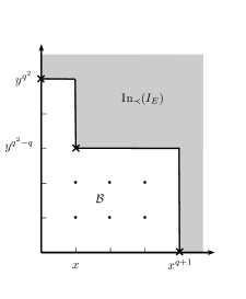
Figure 1. The set of monomials in $\mathcal{B}$

Remark 2.7.

The monomial basis $\mathcal{B}$ for the $\mathbb{F}_{q^{2}}$-vector space $A_{E}$ allows us to represent every class in $A_{E}$ by the unique polynomial $F$ in this class such that its degree $\partial_{x}(F)$ with respect to $x$ is at most $q$ and its degree $\partial_{y}(F)$ with respect to $y$ is at most $q^{2}-1$. We observe that $\prec$ and $<_{w}$ choose the same leading monomial for each polynomial $F$ in $\mathbb{F}_{q^{2}}[x,y]$ such that $\partial_{x}(F)\leq q$.

In fact, let us consider two monomials $x^{\alpha_{1}}y^{\beta_{1}}$ and $x^{\alpha_{2}}y^{\beta_{2}}$ in $\mathcal{B}$ such that $x^{\alpha_{1}}y^{\beta_{1}}\prec x^{\alpha_{2}}y^{\beta_{2}}$. This happens when either $\alpha_{1}+\beta_{1}=\alpha_{2}+\beta_{2}$ and $\alpha_{1}>\alpha_{2}$ or $\alpha_{1}+\beta_{1}<\alpha_{2}+\beta_{2}$.

In the first case we have equality between positive integers $\alpha_{1}-\alpha_{2}=\beta_{2}-\beta_{1}$ and so $(\alpha_{1}-\alpha_{2})q<(\beta_{2}-\beta_{1})(q+1)$, hence $x^{\alpha_{1}}y^{\beta_{1}}<_{w}x^{\alpha_{2}}y^{\beta_{2}}$.
In the second case, we have $\alpha_{1}-\alpha_{2}<\beta_{2}-\beta_{1}$. If $\beta_{2}-\beta_{1}\geq 0$, then $(\alpha_{1}-\alpha_{2})q<(\beta_{2}-\beta_{1})(q+1)$ hence $x^{\alpha_{1}}y^{\beta_{1}}<_{w}x^{\alpha_{2}}y^{\beta_{2}}$. It remains to consider the case $\beta_{1}=\beta_{2}+t$ and $\alpha_{2}=\alpha_{1}+t+k$, with suitable positive integers $t,k$. Then $(\alpha_{1}-\alpha_{2})q-(\beta_{2}-\beta_{1})(q+1)=-kq+t$ which is negative since $t<\alpha_{2}\leq q$.
As a consequence we see that the $w$-degrees of the monomials in $\mathcal{B}$ are pairwise different. Moreover, they cover the range of integers between $0$ and $q^{3}+(q^{2}-q)-1=n+2g-1$, with $2g$ exceptions. In fact there are $g$ integers between $1$ and $2g-1$ that cannot be obtained as the $w$-degree of any monomial: they are the gaps of the semigroup generated by $q$ and $q+1$. Moreover, there are $g$ numbers between $n$ and $n+2g-1$ that are the $w$-degree of monomials multiple of $xy^{q^{2}-q}$ that do not belong to $\mathcal{B}$ since $xy^{q^{2}-q}\in\mathrm{In}_{\prec}(I_{E})$.

Finally, we summarize the explicit construction of the Hermitian code.

Definition 2.8.

Let us fix any ordered list $[P_{1},\dots,P_{n}]$ of the $n$ points of $E$. Let $\mathcal{B}$ be as (2.3), $m$ be any integer $\leq n+2g-2$, and let $V_{m}\subseteq A_{E}$ be the vector space with basis

$$\mathcal{B}_{m}=\mathcal{B}\cap V_{m}=\{x^{r}y^{s}\in\mathcal{B}\mid rq+s(q+1)\leq m\}.$$

Then the Hermitian code $C_{m}$ is the $\mathbb{F}_{q^{2}}$-vector space $(\mathrm{Span}_{\mathbb{F}_{q^{2}}}\langle\phi_{I_{E}}(\mathcal{B}_{m})\rangle)^{\perp}$ where $\phi_{I_{E}}$ is the evaluation map (2.1) at the points of $E$.

The Hermitian codes can be divided in four phases [13], any of them having specific explicit formulas linking their dimension and their distance [24], as in Table 1.

Table 1. The four “phases”of Hermitian codes [24].

Phase	m	Distance d	Dimension k
1	$\begin{array}[]{c}0\leq m\leq q^{2}-2\\ m=aq+b\\ 0\leq b\leq a\leq q-1\\ b\neq q-1\end{array}$	$\begin{array}[]{ll}a+1&a>b\\ a+2&a=b\end{array}\iff d\leq q$	$q^{3}-\frac{a(a+1)}{2}-(b+1)$
2	$\begin{array}[]{c}q^{2}-1\leq m\leq 4g-3\\ m=(2g-2)+aq-b\\ 2\leq a\leq q-1\\ 0\leq b\leq q-2\\ \mbox{ if }a=q-1\mbox{ then }b\geq 1\end{array}$	$\begin{array}[]{ll}aq-b&\mbox{ if }aq-b\in\langle q,q+1\rangle\\ aq&\mbox{ if }aq-b\not\in\langle q,q+1\rangle\end{array}$	$n-m+g-1$
3	$4g-2\leq m\leq n-2$	$m-2g+2$	$n-m+g-1$
4	$\begin{array}[]{c}n-1\leq m\leq n+2g-2\\ m=n+2g-2-aq-b\\ 0\leq b\leq a\leq q-2,\end{array}$	$n-aq-b$	$\frac{a(a+1)}{2}+b+1$

3. Hermitian codes $C_{m}$ with $m\geq q^{2}-1$.

In the following, for every Hermitian code $C_{m}$ with $m\geq q^{2}-1$, we will denote by $(\mu,\beta)$ the unique pair of non negative integers such that $m=\mu q+\beta(q+1)$ and $\mu\leq q$ (Remark 2.7). As we are considering only the case $m\geq q^{2}-1$, these integers do exist.

It is a straightforward consequence of Definition 2.8 that $C_{m}\supseteq C_{m^{\prime}}$ when $m<m^{\prime}$. If in $\mathcal{B}$ there is no monomial of $w$-degree $m+1$, then $\mathcal{B}_{m}=\mathcal{B}_{m+1}$ and there is only one code corresponding to $m$ and to $m+1$. For this reason we adopt the following

Convention 3.1.

We will label a code after an integer $m$ if and only if $\mathcal{B}$ contains a monomial of $w$-degree $m+1$.

Therefore, by Remark 2.7, we do not label a code after $m$ when either $m+1$ is a gap of the semigroup $\langle q,q+1\rangle$ or the only monomial $x^{r}y^{s}$ with $r\leq q$ and $w$-degree $m+1$ is a multiple of $xy^{q^{2}-q}$.

Example 3.2.

For $q=3$, the first integer $m$ in the rang of the fourth phase is $26$. However, we do not label any code after this value of $m$. In fact, the only monomial $x^{r}y^{s}$ with $r\leq 3$ and $w$-degree $26+1$, is $xy^{6}$, a minimal generator of $\mathrm{In}_{\prec}(I_{E})=\langle x^{4},xy^{6},y^{9}\rangle$. Hence, $\mathcal{B}_{26}=\mathcal{B}_{27}$. On the other hand, in $\mathcal{B}$ there is the monomial $y^{7}$ whose $w$-degree is $27+1$, so that $\mathcal{B}_{27}\neq\mathcal{B}_{28}$. Therefore, the first code of the fourth phase will be denoted in our convention as $C_{27}$.

Note that for every monomial $x^{r}y^{s}$ of $\mathcal{B}$ we have

$$x^{r}y^{s}\in\mathcal{B}\setminus\mathcal{B}_{m}\Longleftrightarrow\mbox{ either }r+s>\mu+\beta\hbox{ or }r+s=\mu+\beta\hbox{ and }r<\mu.$$

In the following, for any $\mathbb{F}_{q^{2}}$-divisor $D$ over the Hermitian curve we will denote by $V_{m,D}$ the image of $V_{m}$ in $A_{D}$. We observe that $D$ contains the support of some codeword of $C_{m}$ if $V_{m,D}$ has dimension less than $|D|$. We summarize all these facts in the following:

Proposition 3.3.

Let $D$ be a $\mathbb{F}_{q^{2}}$-divisor over the Hermitian curve. Then the following are equivalent for the Hermitian code $C_{m}$ with $m\geq q^{2}-1$:

1. $\exists\ \mathbf{c}\in C_{m}$ with $\mathbf{c}\neq 0$ such that $\mathrm{Supp}(\mathbf{c})\subseteq D$

2. $V_{m,D}$ has dimension less than $|D|$ as $\mathbb{F}_{q^{2}}$-vector space.

3. There exists a monomial $x^{a}y^{b}\in\mathcal{N}(\mathrm{In}_{\prec}(I_{D}))$ whose $w$-degree $w(x^{a}y^{b})=aq+b(q+1)$ satisfies $m+1\leq w(x^{a}y^{b})\leq m+q+1$.

4. Let $m=\mu q+\beta(q+1)$. If $\mu>0$, $\mathcal{N}(\mathrm{In}_{\prec}(I_{D}))$ contains at least one monomial in

   (3.1) $$\mathcal{L}_{1}:=\{x^{\mu-i}y^{\beta+i}\hbox{ with }1\leq i\leq\mu\}\cup\{x^{q-j}y^{\beta+\mu-q+j+1}\hbox{ with }0\leq j\leq q-\mu\};$$

   otherwise, $\mu=0$ and $\mathcal{N}(\mathrm{In}_{\prec}(I_{D}))$ contains at least one monomial in

   (3.2) $$\mathcal{L}_{2}:=\{x^{q-j}y^{\beta-q+j+1},\hbox{ with }0\leq j\leq q\}.$$

Proof.

Let $\rm H_{E}$ be the parity-check matrix of the repetition code (the only one with distance $q^{3}$, whose codewords are the $q^{2}$ vectors with all the entries pairwise equal) and $\rm H_{E,m}$ be the parity-check matrix of the code $C_{m}$. Let us consider their sub-matrices $M_{D}$ and $M_{D,m}$ obtained only considering the columns corresponding to the points $P_{i}\in D$. More explicitly, if $\delta=|D|$ and $D=\{P_{i_{1}},\dots,P_{i_{\delta}}\}$ the $j$-th column of $\rm H_{E}$ (respectively of $\rm H_{E,m}$) is formed by the evaluation of the monomials of $\mathcal{B}$ (respectively of $\mathcal{B}_{m}$) at $P_{i_{j}}$.
The codewords of $C_{m}$ are the solutions of the homogeneous linear system $\rm H_{E,m}\cdot Z^{T}=0$, where $Z=(z_{1},\dots,z_{n})$. The list of non-zero components of any codeword $\mathbf{c}\in C_{m}$ with $\mathrm{Supp}(\mathbf{c})\subseteq D$ is a solution of the linear system $M_{D,m}\cdot Z_{D}^{T}=0$, where $Z_{D}=(z_{i_{1}},\dots,z_{i_{\delta}})$. Therefore, there exist non-zero codewords $\mathbf{c}\in C_{m}$ such that $\mathrm{Supp}(\mathbf{c})\subseteq D$ if and only if $\mathrm{rk}(M_{D,m})<|D|$, that is, ((ii)) is verified.
By Lemma 2.6 the basis of $A_{D}$ given by the monomials of $\mathcal{N}(\mathrm{In}_{\prec}(I_{D}))$ is a subset of $\mathcal{B}$. Since $\mathrm{rk}(M_{D})=|D|$, then ((i)) is verified if and only if there exists a monomial $x^{r}y^{s}\in\mathcal{B}\setminus\mathcal{B}_{m}$ that belongs to $\mathcal{N}(\mathrm{In}_{\prec}(I_{D}))$. We may assume that $x^{r}y^{s}$ is the monomial in $\mathcal{N}(\mathrm{In}_{\prec}(I_{D}))\cap(\mathcal{B}\setminus\mathcal{B}_{m})$ having minimum $w$-degree.

This $w$-degree is less than or equal to $m+q+1$. In fact, if this were not true we could find in $\mathcal{N}(\mathrm{In}_{\prec}(I_{D}))$ either $x^{r-1}y^{s}$ or $x^{r}y^{s-1}$ with $w$-degree still larger than $m$ against the minimality of $x^{r}y^{s}$.
The equivalence between ((iii)) and ((iv)) is obvious, being ((iv)) a more explicit rewriting of ((iii)). ∎

Observe that the equivalence between the conditions ((i)),((ii)),((iii)) holds true for every Hermitian code $C_{m}$ and also ((iv)) is equivalent to the previous ones provided the integer $m$ can be written as $\mu q+\beta(q+1)$.

3.1. Complete intersections on $\mathcal{H}$

In this section we use the Bézout Theorem to find some properties of the zero-dimensional schemes that are complete intersection of $\mathcal{H}$ with another curve $\mathcal{X}$. To this purpose, we must also consider the possible intersections at infinity. We recall that the projective closure $\overline{\mathcal{H}}$ of $\mathcal{H}$ has a single point at infinity $P_{\infty}=[x_{0}=0:x_{1}=0:x_{2}]$ where $x_{1}/x_{0}=x$ and $x_{2}/x_{0}=y$. It is a smooth, inflexion point with tangent line $x_{0}=0$.

Proposition 3.4.

Let $F\in\mathbb{F}_{q^{2}}[x,y]$ be a polynomial such that $\partial_{x}(F)\leq q$ and let $\mathcal{X}$ be the curve given by the ideal $\langle F\rangle$. If $\mathrm{LM}_{\prec}(F)=x^{r}y^{s}$, then

1. $\mathrm{In}_{\prec}(\langle H,F\rangle)=\langle x^{q+1},x^{r}y^{s},y^{s+q}\rangle$ when $s>0$ and

2. $\mathrm{In}_{\prec}(\langle H,F\rangle)=\langle x^{r},y^{q}\rangle$ when $s=0$.

Moreover, the degree of the divisor $D$ cut on $\mathcal{H}$ by $\mathcal{X}$ is $rq+s(q+1)$.

Proof.

We first prove that $|D|=rq+s(q+1)$. Since the term ordering $\prec$ is degree-compatible, the degree of $F$ is equal to the degree $r+s$ of its leading monomial. By Bézout Theorem, the degree of the divisor $\overline{D}$ cut on $\overline{\mathcal{H}}$ by the projective closure $\overline{\mathcal{X}}$ of $\mathcal{X}$ is $(r+s)(q+1)$. It remains to prove that the intersection multiplicity of the two curves at $P_{\infty}$ is $r$. For the generalities about the intersection multiplicity of two plane curves we refer to [fulton:curve].

To this aim, we study the intersection of the two curves looking at any open subset of $\mathbb{P}^{2}$ around $P_{\infty}$; for instance we choose the affine chart given by $x_{2}\neq 0$.

In order to obtain the equations defining the two curves in this affine chart we homogenize $F$ and $H$, by setting $\overline{F}:=F(x_{1}/x_{0},x_{2}/x_{0})\cdot x_{0}^{r+s}$ and $\overline{H}:=H(x_{1}/x_{0},x_{2}/x_{0})\cdot x_{0}^{q+1}=x_{1}^{q+1}-x_{2}^{q}x_{0}-x_{2}x_{0}^{q}$. Then we de-homogenize by setting $x_{2}=1,x_{0}=z,x_{1}=x$ and get the wanted equations $F^{\prime}$ and $H^{\prime}=x^{q+1}-z^{q}-z$. For what concerns $F^{\prime}$, we observe that all monomials of maximum degree in the support of $F$ are divisible by $x^{r}$; hence every monomial of $F^{\prime}$ is divisible by $z$ and/or by $x^{r}$. Furthermore, the monomial $x^{r}$ appears in the support of $F^{\prime}$, since $x^{r}y^{s}$ is in the support of $F$ and we have performed the following transformations

$$x^{r}y^{s}\mapsto\frac{x_{1}^{r}}{x_{0}^{r}}\cdot\frac{x_{2}^{s}}{x_{0}^{s}}\cdot x_{0}^{r+s}=x_{1}^{r}x_{2}^{s}\mapsto x^{r}.$$

Without modifying the intersection multiplicity at $P_{\infty}$, we can replace any occurrence of $z$ in $F^{\prime}$ by $H^{\prime}+z=x^{q+1}-z^{q}$, and repeat this substitution until we get a polynomial $F^{\prime\prime}$ having $x^{r}$ as the only monomial of minimum degree. Therefore, $mult_{P_{\infty}}(\overline{\mathcal{H}},\overline{\mathcal{X}})=mult_{P_{\infty}}(H^{\prime},F^{\prime})=mult_{P_{\infty}}(H^{\prime},F^{\prime\prime})=r$.

This allows us to conclude that $|D|=|\overline{D}|-|rP_{\infty}|=rq+s(q+1)$.

Now we prove ((i)) and ((ii)). As the set of monomials $\mathcal{N}(\mathrm{In}_{\prec}(I_{D}))$ is a basis for $A_{D}$, for what just proved we know that its cardinality is $rq+s(q+1)$.

• If $s>0$, we can write $F$ as $x^{r}y^{s}+x^{r+1}F_{1}+F_{2}$ where $\partial F_{1}=s-1$ and $\partial F_{2}<r+s$. We observe that the polynomial $x^{q+1-r}F-(y^{s}+xF_{1})H$ is an element of $I_{D}$ and its leading monomial is $y^{s+q}$. Therefore, $\mathrm{In}_{\prec}(I_{D})\supseteq J:=\langle x^{q+1},x^{r}y^{s},y^{s+q}\rangle$, so that $\mathcal{N}(\mathrm{In}_{\prec}(I_{D}))\subseteq\mathcal{N}(J)$. It is now easy to check that the cardinality of $\mathcal{N}(J)$ is exactly $rq+s(q+1)$ and get the equality $\mathrm{In}_{\prec}(I_{D})=J$.

• If $s=0$ we can write $F$ as $x^{r}+F_{3}$ where $\partial F_{3}<r$. Again, we see that the polynomial $H-x^{q+1-r}F$ belongs to $I_{D}$ and its leading monomial is $y^{q}$. Hence $\mathrm{In}_{\prec}(I_{D})\supseteq J^{\prime}:=\langle x^{r},y^{q}\rangle$, so that $\mathcal{N}(\mathrm{In}_{\prec}(I_{D}))\subseteq\mathcal{N}(J^{\prime})$. An easy computation shows that $|\mathcal{N}(J^{\prime})|=rq$ and we conclude that $\mathrm{In}_{\prec}(I_{D})=J^{\prime}$.

∎

Corollary 3.5.

Let $D$ be a divisor over $\mathcal{H}$ and let $x^{r}y^{s}$ be a monomial in $\mathrm{In}_{\prec}(I_{D})$ with $r\leq q$. Then $|D|\leq rq+s(q+1)$.

Proof.

Let $F$ be any polynomial in $I_{D}$ such that $\mathrm{LM}_{\prec}(F)=x^{r}y^{s}$. Then the degree of $F$ is $r+s$ and the projective closure of the curve defined by $F$ cuts on $\overline{\mathcal{H}}$ a divisor $D+D^{\prime}+tP_{\infty}$ of degree $(r+s)(q+1)$. By Proposition 3.4 we know that $t=r$ and so $|D|\leq|D+D^{\prime}|=(r+s)(q+1)-r=rq+s(q+1)$. ∎

Lemma 3.6.

Let $D$ be a $\mathbb{F}_{q^{2}}$-divisor over $\mathcal{H}$ which is the support of a non-zero codeword of $C_{m}$. Then $I_{D}$ verifies at least one of the following conditions:

1. $x^{q+1}\in\mathrm{In}_{\prec}(I_{D})$ and $x^{q}\notin\mathrm{In}_{\prec}(I_{D})$

2. $y^{q}\in\mathrm{In}_{\prec}(I_{D})$.

If moreover $m\geq 2q^{2}-2q-2$, then either $x^{q}\notin\mathrm{In}_{\prec}(I_{D})$, or $y^{q-1}\notin\mathrm{In}_{\prec}(I_{D})$.

Proof.

Since $I_{D}$ is a zero-dimensional ideal, then $\mathrm{In}_{\prec}(I_{D})$ contains some power of $x$ and of $y$: let $x^{r}$ and $y^{s}$ be the minimal ones. Obviously, $r\leq q+1$, as $H\in I_{D}$. We assume $r\leq q$, and prove that $s\leq q$.

Indeed, if $F$ is any polynomial in $I_{D}$ with leading monomial $x^{r}$, then we find in $I_{D}$ also the polynomial $H-x^{q+1-r}F$ whose leading monomial is $y^{q}$.
It remains to prove that when $m\geq 2q^{2}-2q-2$ we cannot have both $r\leq q$ and $s\leq q-1$. In fact, if so, $\mathrm{In}_{\prec}(I_{D})\supseteq\langle x^{q},y^{q-1}\rangle$, that is $\mathcal{N}(\mathrm{In}_{\prec}(I_{D}))\subseteq\mathcal{N}(\langle x^{q},y^{q-1}\rangle)$. The larger $w$-degree of monomials in $\mathcal{N}((x^{q},y^{q-1}))$ is $w(x^{q-1}y^{q-2})=2q^{2}-2q-2\leq m$, in contradiction with Proposition 3.3. ∎

4. Minimum distance of Hermitian codes of third and fourth phase

In this section we study the Hermitian codes $C_{m}$ with $m\geq 2q^{2}-2q-2$ and in particular, at the end of the section, we get a formula for their distance. What we obtain is nothing else than the well known formula first proved by Stichtenoth in [34]. However, we prefer to prove it directly since the preliminary results that will lead us to this proof, especially Theorem 4.2, are key tools in the main results of this paper.

Remark 4.1.

We observe that in the new hypothesis, the numbers $\mu$ and $\beta$ such that $m=\mu q+\beta(q+1)$ always satisfy the inequalities $0\leq\mu\leq q$ and $\beta\geq q-2$. More generally if $a,b$ are non-negative integers such that $a\leq q$ and $aq+b(q+1)\geq 2q^{2}-2q-2$, then $b\geq q-2$.

The argument we use to prove the last part of the following theorem is directly inspired by the one used by Stichtenoth in [34] to explicitly exhibit some codewords of minimum weight and exploit the norm-trace form of the equation of $\mathcal{H}$.

Theorem 4.2.

Let $x^{a}y^{b}\in\mathcal{B}\setminus\mathcal{B}_{m}$ such that $m+1\leq w(x^{a}y^{b})\leq m+q+1$.

1. If $D$ is a $\mathbb{F}_{q^{2}}$-divisor over $\mathcal{H}$ such that $x^{a}y^{b}\in\mathcal{N}(\mathrm{In}_{\prec}(I_{D}))$ and which is the support of a codeword of $C_{m}$, then $|D|\geq w(x^{a}y^{b})-(q^{2}-q)+1$.

2. There exists a $\mathbb{F}_{q^{2}}$-divisor $D^{\prime}$ over $\mathcal{H}$ corresponding to a codeword of $C_{m}$ such that $x^{a}y^{b}\in\mathcal{N}(\mathrm{In}_{\prec}(I_{D^{\prime}}))$ and $|D^{\prime}|=w(x^{a}y^{b})-(q^{2}-q)+1$.

Proof.

By Remark 4.1 we have that $0\leq a\leq q$ and $b\geq q-2$. We split the proof of the first item into three cases:

• If $b=q-2$, then $w(x^{a}y^{b})\geq m+1$ if and only if $a=q$. Since $x^{a}y^{b}=x^{q}y^{q-2}\in\mathcal{N}(\mathrm{In}_{\prec}(I_{D}))$, then $\mathcal{N}(\mathrm{In}_{\prec}(I_{D}))$ also contains all $(q+1)(q-1)$ factors of $x^{q}y^{q-2}$. Therefore, $|D|=|\mathcal{N}(\mathrm{In}_{\prec}(I_{D}))|\geq(q+1)(q-1)=w(x^{a}y^{b})-(q^{2}-q)+1$.

• If $b=q-1$, we can argue as in the previous case: from $x^{a}y^{q-1}\in\mathcal{N}(\mathrm{In}_{\prec}(I_{D}))$ we get $|D|=|\mathcal{N}(\mathrm{In}_{\prec}(I_{D}))|\geq(a+1)q=w(x^{a}y^{b})-(q^{2}-q)+1$.

• If $b\geq q$, then $y^{q}\notin\mathrm{In}_{\prec}(I_{D})$. As a consequence, we know by Lemma 3.6 that $x^{q+1}$ is the minimal power of $x$ in $\mathrm{In}_{\prec}(I_{D})$ and we deduce by Proposition 3.4 that $x^{q}y^{b-q}\not\in\mathrm{In}_{\prec}(I_{D})$.

  Computing the number of factors of the two monomials $x^{a}y^{b}$ and $x^{q}y^{b-q}$ we get $|D|=|\mathcal{N}(\mathrm{In}_{\prec}(I_{D}))|\geq(a+1)(b+1)+(q+1)(b-q+1)-(a+1)(b-q+1)=w(x^{a}y^{b})-(q^{2}-q)+1$.

Now we prove the second item, again splitting in cases. In all of them we can obtain $D^{\prime}$ as the divisor cut on $\mathcal{H}$ by a curve $\mathcal{Y}$ union of lines chosen among those cutting on $\mathcal{H}$ an $\mathbb{F}_{q^{2}}$-divisor. Recall that there are $q^{2}$ vertical lines $\mathcal{L}_{i}$, each containing $q$ points of $E$, and $q^{2}-q+1$ horizontal lines $\mathcal{L}^{\prime}_{j}$, each containing $q+1$ points of $E$ (Remark 2.1).

• If $a=q$ and $b\in\{q-2,q-1\}$, $\mathcal{Y}$ is the union of $b+1$ horizontal lines $\mathcal{L}^{\prime}_{j}$, so that $\mathrm{In}_{\prec}(I_{D^{\prime}})=\langle x^{q+1},y^{b+1}\rangle$.

• If $a=b=q-1$, $\mathcal{Y}$ is the union of $q$ vertical lines $\mathcal{L}_{i}$, so that $\mathrm{In}_{\prec}(I_{D^{\prime}})=\langle x^{q},y^{q}\rangle$.

• If $b\geq q$, $\mathcal{Y}$ is the union of $a+1$ vertical lines $\mathcal{L}_{i}$ and $b+1-q$ horizontal lines $\mathcal{L}_{j}^{\prime}$ such that not two of them meet in a point of $E$.
  For instance we can choose among the $\mathcal{L}_{i}$ a set of lines $x$, $x-\alpha_{1},\dots,x-\alpha_{a}$ with $\mathrm{N}(\alpha_{i}):=\alpha_{i}^{q}=1$ and among the $\mathcal{L}_{j}^{\prime}$ a set of lines $y-\beta_{1},\dots,y-\beta_{b+1-q}$ with $\mathrm{Tr}(\beta_{j}):=\beta_{j}^{q+1}-\beta_{j}\neq 0,1$. In this case, we have $\mathrm{In}_{\prec}(I_{D^{\prime}})=\langle x^{q+1},y^{b+1},x^{a+1}y^{b+1-q}\rangle$.

∎

We can now prove a general formula for the distance of the codes of the third and fourth phase.

Corollary 4.3.

The distance of an Hermitian code $C_{m}$ with $m\geq 2q^{2}-2q-2$ is $d=m-q^{2}+q+2=m-2g+2$.

Proof.

By Proposition 3.3, if $D$ is a $\mathbb{F}_{q^{2}}$-divisor over $\mathcal{H}$ corresponding to a codeword of $C_{m}$, then $\mathcal{N}(\mathrm{In}_{\prec}(I_{D}))$ contains a monomial $x^{a}y^{b}$ of $\mathcal{B}\setminus\mathcal{B}_{m}$. By Theorem 4.2, we have $|D|\geq w(x^{a}y^{b})-q^{2}+q+1$, and there is a $\mathbb{F}_{q^{2}}$-divisor $D^{\prime}$ over $\mathcal{H}$ for which we have equality. Therefore, the minimum $w$-degree of such divisors, namely the distance $d$ of the code $C_{m}$, is that obtained when $x^{a}y^{b}$ is the monomial of $w$-degree in $\mathcal{B}\setminus\mathcal{B}_{m}$, that in our assumption is always $m+1$. ∎

Note that the formula given in the previous corollary coincides with that of [13], taking in account Convention 3.1 on the integers $m$ labeling a code. Let for instance $C$ be the first code of the fourth phase (with $q$=3) as in Example 3.2. It corresponds to $\mathcal{B}_{26}=\mathcal{B}_{27}$ so that it could be labeled after both values $m=26$ and $m=27$. We choose to label it as $C_{27}$ and the formula in Corollary 4.3 gives for $m=27$ the correct distance $d=23$ (while $m=26$ would not).

5. Geometric description of minimum weight codewords

In this section we consider Hermitian codes $C_{m}$ with $2q^{2}-2q-2\leq m\leq n+2g-2$.

By Remark 4.1 and Corollary 4.3, there is a unique writing of $m$ as $\mu q+\beta(q+1)$ with $0\leq\mu\leq q$, $\beta\geq q-2$, and the distance of $C_{m}$ is $d=\mu q+\lambda(q+1)$ where $\lambda=\beta-q+2$. Moreover, $\mathcal{B}$ contains only one monomial $x^{a}y^{b}$ with $w$-degree $m+1$.

Theorem 5.1.

Let $C_{m}$ be an Hermitian code, and let $m$, $\mu$, $\beta$, $\lambda$, $a$, $b$ be as above.

1. Let $D$ be a $\mathbb{F}_{q^{2}}$-divisor cut on $\mathcal{H}$ by the curve defined by a polynomial $F$ such that $\mathrm{LM}_{\prec}(F)=x^{\mu}y^{\lambda}$. Then $D$ corresponds to minimum weight codewords of $C_{m}$.

2. Let $D$ be a $\mathbb{F}_{q^{2}}$-divisor on $\mathcal{H}$ corresponding to minimum weight codewords of $C_{m}$. Then $\mathcal{N}(\mathrm{In}_{\prec}(I_{D}))$ contains only one monomial with $w$-degree larger than $m$, the monomial $x^{a}y^{b}$, with $w$-degree exactly equal to $m+1$. Moreover $D$ is cut on $\mathcal{H}$ by the curve defined by a polynomial $F$ such that $\mathrm{LM}_{\prec}(F)=x^{\mu}y^{\lambda}$.

Proof.

1. By Proposition 3.4, if $D$ is a $\mathbb{F}_{q^{2}}$-divisor cut on $\mathcal{H}$ by the curve defined by a polynomial $F$ such that $\mathrm{LM}_{\prec}(F)=x^{\mu}y^{\lambda}$, then $|D|=\mu q+\lambda(q+1)$. Moreover, if $\lambda\geq 1$, then $\mathrm{LM}_{\prec}(\langle H,F\rangle)=\langle x^{q+1},x^{\mu}y^{\lambda},y^{\lambda+q}\rangle$; otherwise $\lambda=0$ and $\mathrm{In}_{\prec}(\langle H,F\rangle)=\langle x^{\mu},y^{q}\rangle$. In both cases, $\mathcal{N}(\mathrm{In}_{\prec}(I_{D}))$ contains a monomial of $w$-degree $m+1$. By Proposition 3.3, $D$ corresponds to codewords of weight $|D|=d$.

2. It is easy to see that $x^{a}y^{b}=x^{\mu-1}y^{\lambda+q-1}$ if $\mu\geq 1$, and $x^{a}y^{b}=x^{q}y^{\lambda-1}$ if $\mu=0$. Moreover, by Theorem 4.2, among the $d$ monomials of $\mathcal{N}(\mathrm{In}_{\prec}(I_{D}))$ we find $x^{a}y^{b}$ and all its factors: then $d\geq\mu(\lambda+q)$ if $\mu\geq 1$ and $d\geq(q+1)\lambda$ if $\mu=0$.

   

   

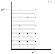
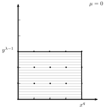
   Figure 2. The divisors of $x^{\mu-1}y^{\lambda+q-1}$ when $\mu\geq 1$ and of $x^{q}y^{\lambda-1}$ if $\mu=0$.

   We consider tree different cases:

   • Case $\mu=0$. Since $d=\lambda(q+1)$, the number of monomials dividing $x^{a}y^{b}$ are exactly as many as the monomials in $\mathcal{N}(\mathrm{In}_{\prec}(I_{D}))$, hence $\mathcal{N}(\mathrm{In}_{\prec}(I_{D}))$ is exactly the set of these monomials. Therefore, there exist a polynomial $F$ in $I_{D}$ such that $LM_{\prec}(F)=y^{\lambda}$. By Corollary 3.5 this polynomial cuts on $\mathcal{H}$ a divisor $D^{\prime}$ which contains $D$ and has the same degree of $D$, so $D^{\prime}=D$.

   • Case $\mu,\lambda>0$. We observe that $x^{q}y^{\lambda-1}$ must belong to $\mathcal{N}(\mathrm{In}_{\prec}(I_{D}))$. Otherwise, by Proposition 3.4, we would $y^{\lambda+q-1}\in\mathrm{In}(I_{D})$ and so also $x^{\mu-1}y^{\lambda+q-1}\in\mathrm{In}_{\prec}(I_{D})$, against what we have just proved.

     

     Figure 3. The number of monomials in $\mathcal{N}(\mathrm{In}_{\prec}(\langle H,F\rangle))$.

     Computing the number of the divisors of $x^{\mu-1}y^{\lambda+q-1}$ and of $x^{q}y^{\lambda-1}$, we get exactly $d$ (see Figure 3). Therefore, $\mathcal{N}(\mathrm{In}_{\prec}(I_{D}))$ is formed by these monomials, since $|\mathcal{N}(\mathrm{In}_{\prec}(I_{D}))|=d$. Moreover $x^{\mu}y^{\lambda}$, that does not divide neither $x^{\mu-1}y^{\lambda+q-1}$ nor $x^{q}y^{\lambda-1}$, belongs to $\mathrm{In}_{\prec}(I_{D})$. Then, there is a polynomial $F\in I_{D}$ with leading monomial $x^{\mu}y^{\lambda}$. By Corollary 3.5 the curve defined by $F$ cuts $D$ on $\mathcal{H}$.

   • Case $\lambda=0$. The monomial $x^{a}y^{b}=x^{\mu-1}y^{q-1}$ has exactly $\mu q=d$ divisors. So $\mathcal{N}(\mathrm{In}_{\prec}(I_{D}))$ is formed by these monomials. Therefore $x^{\mu}$ is an element of $\mathrm{In}_{\prec}(I_{D}))$. If $F\in I_{D}$ has leading monomial $x^{\mu}$, by Proposition 3.4, $I_{D}$ contains the ideal generated by $H$ and $F$ whose initial ideal is $(x^{\mu},y^{q})$. So $I_{D}=(H,F)$ and the curve defined by $F$ cuts $D$ on $\mathcal{H}$.

∎

Remark 5.2.

Let $C_{m}$ be the Hermitian code with distance $d=\mu q+\lambda(q+1)$. As shown in the proof of Theorem 4.2, we obtain some divisor $D$ corresponding to a minimum-weight codeword of $C_{m}$ cutting $\mathcal{H}$ with a suitable curve $\mathcal{X}$ union of $\mu$ vertical lines and $\lambda$ horizontal lines, so that the leading monomial of the polynomial defining such a curve $\mathcal{X}$ is indeed $x^{\mu}y^{\lambda}$.
On the other hand, we point out that not all the polynomials $F$ in $\mathbb{F}_{q^{2}}[x,y]$ with leading monomial $x^{\mu}y^{\lambda}$ correspond to minimum-weight codewords of the code $C_{m}$. The following result contains an explicit characterization of the “good”polynomials as a consequence of Remark 2.3.

Corollary 5.3.

Let $C_{m}$ be the Hermitian code with distance $d=\mu q+\lambda(q+1)$. A polynomial $F$ over $\mathbb{F}_{q^{2}}$ with $\mathrm{LM}_{\prec}(F)=x^{\mu}y^{\lambda}$ cuts over $\mathcal{H}$ a divisor $D$ corresponding to minimum-weight codewords if and only if the ideal $\langle H,F\rangle$ contains the field equations $x^{q^{2}}-x$ and $y^{q^{2}}-y$.

6. Algorithm to compute the number of minimum-weight codewords

Let $C_{m}$ be an Hermitian code of either third or fourth phase. Based on the results obtained in the previous sections, and mainly on Theorem 5.1, we now describe an algorithm computing the number $\texttt{MW}_{m}$ of minimum-weight codewords of $C_{m}$ can be built. Then, we propose Algorithm 1 which takes as inputs $q,m$, and returns $\texttt{MW}_{m}$.

We know that the integer $m$ such that $C_{m}$ is a code in ether the third or the fourth phase can be written as $m=\mu q+(\lambda+q-2)(q+1)$ with $\mu$, $\lambda$ non-negative integers and $\mu\leq q$; moreover we know a formula giving the distance of $C_{m}$ as a function of $\lambda$ and $\mu$. We identify the code $C_{m}$ with the triple of integers $(q,\lambda,\mu)$. We recall that $\prec$ denotes the term ordering $\mathtt{DegRevLex}$ in $\mathbb{F}_{q^{2}}[x,y]$ with $y>x$.

• We compute the distance $d=\mu q+\lambda(q+1)$ of the code $C_{m}$.

• We compute the set $M$ of the pairs $(a,b)$ of exponents of the monomials $x^{a}y^{b}$ such that $x^{a}y^{b}\prec x^{\mu}y^{\lambda}$ and $a\leq q$.

• Now we exploit Theorem 5.1. For every monomial $(a,b)$ in $M$, we introduce a variable $\nu_{a,b}$. Then we set

  $$f:=x^{\mu}y^{\lambda}+\sum_{(a,b)\in M}\nu_{a,b}x^{a}y^{b}.$$

  (line 4 of Algorithm 1).

• We compute the Gröbner basis $\mathcal{G}(I)$ of the ideal $I=\langle f,H\rangle$ in $\mathbb{F}_{q^{2}}[T,x,y]$, where $T=\{\nu_{a,b}\}_{(a,b)\in M}$, w.r.t a block term ordering that is $\mathtt{DegRevLex}$ with $y>x$ for the first block $\{y,x\}$ and is any term ordering on the second block $T$. Note that, by Proposition 3.4 we obtain a Gröbner basis $\mathcal{G}(I)$ formed by two or three polynomials whose leading monomials only contains the variables $x,y$ (line 6 of Algorithm 1).

• We compute the normal forms $N_{x}$ of $x^{q^{2}}-x$ and $N_{y}$ of $y^{q^{2}}-y$ with respect to $\mathcal{G}(I)$ (lines 7-8 of Algorithm 1). By Remark 2.3, a specialization of the coefficients $\nu_{a,b}$ in $\mathbb{F}_{q^{2}}$ corresponds to a curve that cuts on $\mathcal{H}$ an $\mathbb{F}_{q^{2}}$-divisor if and only if under this specialization the ideal $I$ contains the polynomials $x^{q^{2}}-x$ and $y^{q^{2}}-y$, hence if and only if the normal forms $N_{x}$ and $N_{y}$ vanish.

• We collect the two normal forms w.r.t. the variables $x,y$ and coefficients in $\mathbb{F}_{q^{2}}[T]$ and construct the ideal $J$ in $\mathbb{F}_{q^{2}}[T]$ generated by the coefficients of the two normal forms and by the field equations $\nu_{a,b}^{q^{2}}-\nu_{a,b}$ for every $\nu_{a,b}\in T$ (line 9 of Algorithm 1).

• By Remark 2.3, $J$ is the reduced ideal of a finite set of points $\mathcal{V}(J)$ in $\mathbb{A}_{\mathbb{F}_{q^{2}}}^{N}$, where $N=|T|$. We compute the cardinality of $\mathcal{V}(J)$ computing either all its elements or the constant $z$ which is the affine Hilbert polynomial of $\mathbb{F}_{q^{2}}[T]/J$ (line 10 of Algorithm 1).

• The set of points in $\mathcal{V}(J)$ corresponds to the set of minimum-weight codewords of $C_{m}$. More precisely, to each point in $\mathcal{V}(J)$ we associate an homogeneous linear system whose solutions form a $1$-dimensional $\mathbb{F}_{q^{2}}$-vector space and (except the zero one) are minimum-weight codewords of $C_{m}$. Therefore, the number $\texttt{MW}_{m}$ of minimum-weight codewords of $C_{m}$ is $|\mathcal{V}(J)|\cdot(q^{2}-1)=z\cdot(q^{2}-1)$ (line 11 of Algorithm 1).

Let us suppose that the following functions are available (they are present in the libraries for most computer algebra softwares as for instance MAGMA):

• GroebnerBasis$(I)$ computing the Gröbner basis $\mathcal{G}(I)$ of the ideal $I$ w.r.t. the term ordering $\mathtt{DegRevLex}$.

• NormalForm$(f,G)$ computing the normal form of $f$ with respect to the Gröbner basis $G$.

• HilbertPolynomial$(I)$ computing the affine Hilbert polynomial of a zero-dimensional ideal $I$.

Algorithm 1 Compute the number of minimum-weight codewords

1:function MinimumWords($q,\lambda,\mu$)

2:     $d\leftarrow\mu q+\lambda(q+1)$

3:     $M\leftarrow\{(a,b)\mid a,b\in\mathbb{N},a\leq q,\,aq+b(q+1)<d\}$

4:      $f\leftarrow x^{\mu}y^{\lambda}+\sum_{(a,b)\in M}\nu_{a,b}x^{a}y^{b}$

5:     $I\leftarrow\langle H,f\rangle$

6:      $G\leftarrow\mathtt{GroebnerBasis}(I)$

7:      $N_{x}=\sum_{k,j}\beta_{k,j}x^{k}y^{j}\leftarrow\mathtt{NormalForm}(x^{q^{2}}-x,G)$

8:      $N_{y}=\sum_{\iota,\kappa}\gamma_{\iota,\kappa}x^{\iota}y^{\kappa}\leftarrow\mathtt{NormalForm}(y^{q^{2}}-y,G)$

9:      $J\leftarrow\langle\{\beta_{k,j}\}_{k,j},\{\gamma_{\iota,\kappa}\}_{\iota,\kappa},\{\nu_{a,b}^{q^{2}}-\nu_{a,b}\}_{(a,b)\in M}\rangle$

10:      $z\leftarrow\mathtt{HilbertPolynomial}(J)$

11:      $\texttt{MW}_{m}\leftarrow z\cdot(q^{2}-1)$

12:     return $\texttt{MW}_{m}$.

13:end function

We have implemented this algorithm using the MAGMA software. In MAGMA is already present a function MinimumWords computing the number of minimum-weight codewords. We show in Table 2 and in Table 3 the time needed to compute this number for some codes of the third and fourth phase using the two algorithms. For the computations we used 8 Intel(R) Xeon(R) CPU X5460 $@$ 3.16GHz, 4 core, 32GB of RAM with MAGMA version V2.22-5.

Table 2. Comparison time to compute the number of minimum-weight codewords of $C_{m}$ in the third ($10\leq m\leq 25$) and in fourth phase ($m=27,28$) with $q=3$, using Algorithm 1 and MAGMA command MinimumWords.

$m$	$d$	$\texttt{MW}_{m}$	Algorithm 1	MinimumWords
$10$	$6$	$576$	$\mathbf{0.000}$ s	$15.100$ s
$11$	$7$	$2160$	$\mathbf{0.020}$ s	$163.420$ s
$12$	$8$	$5400$	$\mathbf{0.250}$ s	$191.560$ s
$13$	$9$	$8448$	$\mathbf{2.120}$ s	$68.100$ s
$14$	$10$	$17280$	$9.920$ s	$\mathbf{7.040}$ s
$15$	$11$	$24408$	$119.330$ s	$\mathbf{2.440}$ s
$16$	$12$	$32544$	$467.680$ s	$\mathbf{1.450}$ s
$17$	$13$	$39744$	$1478.540$ s	$\mathbf{1.620}$ s
$18$	$14$	$39744$	$1892.300$ s	$\mathbf{1.230}$ s
$19$	$15$	$32544$	$2073.710$ s	$\mathbf{0.300}$ s
$20$	$16$	$24408$	$3052.910$ s	$\mathbf{0.050}$ s
$21$	$17$	$17280$	$1314.380$ s	$\mathbf{0.040}$ s
$22$	$18$	$8448$	$133.390$ s	$\mathbf{0.020}$ s
$23$	$19$	$5400$	$20.590$ s	$\mathbf{0.010}$ s
$24$	$20$	$2160$	$9.120$ s	$\mathbf{0.010}$ s
$25$	$21$	$576$	$0.470$ s	$\mathbf{0.010}$ s
$27$	$23$	$432$	$0.180$ s	$\mathbf{0.010}$ s
$28$	$24$	$72$	$\mathbf{0.000}$ s	$\mathbf{0.000}$ s

Table 3. Comparison time to compute the number of minimum-weight codewords of $C_{2q^{2}-2q-2}$ with $q=4$, using Algorithm 1 and MAGMA command MinimumWords.

$m$	$d$	$\texttt{MW}_{m}$	Algorithm 1	MinimumWords
$22$	$12$	$150000$	$\mathbf{85.87}$ s	Termination predicted at $10^{16}$ s ($10^{8}$ y)

Note that for the first codes of the third phase, namely the codes $C_{m}$ having lowest $m$, our algorithm is more convenient than MAGMA command MinimumWords. In fact, it improves the running times needing to compute the number of minimum-weight codewords. A striking case is that of $q=4$ and $m=22$ (Table 3), where our algorithm can get the wanted number in $85.87$ seconds while MinimumWords declares that termination requires $10^{8}$ years. The fact that our algorithm shows a better performance for low values of $m$ bodes well for the codes of the second phase.

7. Conclusions and further research

The keystone to finding a geometrical characterization of any minimum-weight codewords for the third and fourth phase was the choice of a different term ordering with respect to what can be usually found in literature, that is the $\mathtt{DegRevLex}$ with $y>x$.

The main novel aspect of our approach was indeed in this deeper attention to the geometry of the problem. For instance, we constructed monomial bases for the quotient ring $A_{E}$ and special subsets of these bases gave rise to the parity-check matrices of the Hermitian codes. These sets of monomials are intrinsically connected to the Hermitian codes themselves, hence we can find them in most papers on the topic. However, the methods used to work with these sets of monomials can be strikingly different. For instance in [26] the authors deal with the problem of computing the number of minimum-weight codewords for the Hermitian codes with distance $d\leq q$ exploiting peculiar methods in linear algebra, as Vandermonde matrices. They find that the minimum-weight codewords are complete intersection of $\mathcal{H}$ and a line of either type $y=ax+b$ or $x=a$. The methods used in [26] appear to be not sufficient to deal with codes with distances larger than the ones considered in their article, as they state in the conclusion of the paper.

“As regards the other phases, it seems that only a part of the second phase can be described in a similar way. Therefore, probably a radically different approach is needed for phase-3, 4 codes in order to determine their weight distribution completely. Alas, we have no suggestions as to how reach this.”

In [27] we have tested our new geometrical approach for codes of phases 1-2, both from a theoretical and a computational point of view, while in the present paper we have tested it for codes of phases 3-4, thus developing the radically different approach sought-after in [26]. We are also confident that this could be a powerful tool also to study the weights distribution of Hermitian codes and to design an efficient algorithm of error detection and correction.

Moreover, there are evidences that complete intersections can provide a good description of codewords with a small weight.

Bibliography

Bibliography

- [1] E. Ballico and C. Marcolla, Higher Hamming weights for locally recoverable codes on algebraic curves, Finite Fields and Their Applications 40 (2016), 61–72.
- [2] E. Ballico and A. Ravagnani, The dual geometry of hermitian two-point codes, Discrete Mathematics 313 (2013), no. 23, 2687–2695.
- [3] by same author, On the geometry of Hermitian one-point codes, Journal of Algebra 397 (2014), 499–514.
- [4] A. I. Barbero and C. Munuera, The weight hierarchy of Hermitian codes, SIAM Journal on Discrete Mathematics 13 (2000), no. 1, 79–104.
- [5] A. Couvreur, The dual minimum distance of arbitrary-dimensional algebraic–geometric codes, Journal of Algebra 350 (2012), no. 1, 84–107.
- [6] C. Fontanari and C. Marcolla, On the geometry of small weight codewords of dual algebraic geometric codes, International Journal of Pure and Applied Mathematics 98 (2015), no. 3, 303–307.
- [7] O. Geil, Evaluation codes from an affine variety code perspective, Advances in algebraic geometry codes, Ser. Coding Theory Cryptol 5 (2008), 153–180.
- [8] O. Geil and T. Høholdt, Footprints or generalized Bezout’s theorem, IEEE Transactions on information theory 46 (2000), no. 2, 635–641.
- [9] O. Geil, S. Martin, R. Matsumoto, D. Ruano, and Y. Luo, Relative generalized Hamming weights of one-point algebraic geometric codes, IEEE Transactions on Information Theory 60 (2014), no. 10, 5938–5949.
- [10] O. Geil and F. Özbudak, Bounding the Minimum Distance of Affine Variety Codes Using Symbolic Computations of Footprints, International Castle Meeting on Coding Theory and Applications, Springer, 2017, pp. 128–138.
- [11] P. Heijnen and R. Pellikaan, Generalized Hamming weights of q-ary Reed-Muller codes, IEEE Trans. Inform. Theory, Citeseer, 1998.
- [12] J.W.P. Hirschfeld, G. Korchmáros, and F. Torres, Algebraic curves over a finite field, Princeton Univ Pr, 2008.
- [13] T. Høholdt, J. H. van Lint, and R. Pellikaan, Algebraic geometry of codes, Handbook of coding theory, Vol. I, II (V. S. Pless and W.C. Huffman, eds.), North-Holland, 1998, pp. 871–961.
- [14] M. Homma and S. J. Kim, Toward the determination of the minimum distance of two-point codes on a Hermitian curve, Designs, Codes and Cryptography 37 (2005), no. 1, 111–132.
- [15] by same author, The complete determination of the minimum distance of two-point codes on a Hermitian curve, Designs, Codes and Cryptography 40 (2006), no. 1, 5–24.
- [16] by same author, The two-point codes on a Hermitian curve with the designed minimum distance, Designs, Codes and Cryptography 38 (2006), no. 1, 55–81.
- [17] by same author, The two-point codes with the designed distance on a Hermitian curve in even characteristic, Designs, Codes and Cryptography 39 (2006), no. 3, 375–386.
- [18] by same author, The second generalized Hamming weight for two-point codes on a Hermitian curve, Designs, Codes and Cryptography 50 (2009), no. 1, 1–40.
- [19] C. Kirfel and R. Pellikaan, The minimum distance of codes in an array coming from telescopic semigroups, IEEE Transactions on information theory 41 (1995), no. 6, 1720–1732.
- [20] K. Lee, Bounds for generalized Hamming weights of general AG codes, Finite Fields and Their Applications 34 (2015), 265–279.
- [21] K. Lee and M. E. O’Sullivan, List decoding of Hermitian codes using Gröbner bases, Journal of Symbolic Computation 44 (2009), no. 12, 1662–1675.
- [22] K. Lee and M. E. O’Sullivan, Algebraic soft-decision decoding of Hermitian codes, Information Theory, IEEE Transactions on 56 (2010), no. 6, 2587–2600.
- [23] J. van Lint and T. Springer, Generalized Reed-Solomon codes from algebraic geometry, IEEE Transactions on Information Theory 33 (1987), no. 3, 305–309.
- [24] C. Marcolla, On structure and decoding of Hermitian codes, Phd thesis, University of Trento, Department of Mathematics, 2013.
- [25] C. Marcolla, E. Orsini, and M. Sala, Improved decoding of affine-variety codes, Journal of Pure and Applied Algebra 216 (2012), no. 7, 1533–1565.
- [26] C. Marcolla, M. Pellegrini, and M. Sala, On the small-weight codewords of some Hermitian codes, Journal of Symbolic Computation (2016), no. 73, 27–45.
- [27] C. Marcolla and M. Roggero, Minimum-weight codewords of the Hermitian codes are supported on complete intersections, Available at arXiv:1605.07827.
- [28] C. Munuera and D. Ramirez, The second and third generalized Hamming weights of Hermitian codes, Information Theory, IEEE Transactions on 45 (1999), no. 2, 709–712.
- [29] M. E. O’Sullivan, Decoding of Hermitian codes: the key equation and efficient error evaluation, Information Theory, IEEE Transactions on 46 (2000), no. 2, 512–523.
- [30] S. Park, Minimum distance of Hermitian two-point codes, Designs, Codes and Cryptography 57 (2010), no. 2, 195–213.
- [31] M. Pellegrini, C. Marcolla, and M. Sala, On the weights of affine-variety codes and some Hermitian codes, Proc. of WCC 2011, Paris (2011), 273–282.
- [32] H. G. Ruck and H. Stichtenoth, A characterization of Hermitian function fields over finite fields, Journal fur die Reine und Angewandte Mathematik 457 (1994), 185–188.
- [33] A. Seidenberg, Constructions in algebra, Trans. Amer. Math. Soc. 197 (1974), 273–313.
- [34] H. Stichtenoth, A note on Hermitian codes over GF(q2), Information Theory, IEEE Transactions on 34 (1988), no. 5, 1345–1348.
- [35] H. Stichtenoth, Algebraic function fields and codes, Universitext, Springer-Verlag, Berlin, 1993.
- [36] H. Tiersma, Remarks on codes from Hermitian curves (corresp.), IEEE transactions on information theory 33 (1987), no. 4, 605–609.
- [37] K. Yang and P. V. Kumar, On the true minimum distance of Hermitian codes, Coding theory and algebraic geometry, Springer, 1992, pp. 99–107.
- [38] K. Yang, P. V. Kumar, and H. Stichtenoth, On the weight hierarchy of geometric Goppa codes, IEEE Transactions on information theory 40 (1994), no. 3, 913–920.