Measurement of the decay $B\to D\ell\nu_{\ell}$ in fully reconstructed events and determination of the Cabibbo–Kobayashi–Maskawa matrix element $|V_{cb}|$

Abstract

We present a determination of the magnitude of the Cabibbo–Kobayashi–Maskawa matrix element $|V_{cb}|$ using the decay $B\to D\ell\nu_{\ell}$ ($\ell=e,\mu$) based on 711$\mbox{~{}fb}^{-1}$ of $e^{+}e^{-}\to\Upsilon(4S)$ data recorded by the Belle detector and containing $772\times 10^{6}$ $B\bar{B}$ pairs. One $B$ meson in the event is fully reconstructed in a hadronic decay mode while the other, on the signal side, is partially reconstructed from a charged lepton and either a $D^{+}$ or $D^{0}$ meson in a total of 23 hadronic decay modes. The isospin-averaged branching fraction of the decay $B\to D\ell\nu_{\ell}$ is found to be $\mathcal{B}(B^{0}\to D^{-}\ell^{+}\nu_{\ell})=(2.31\pm 0.03(\mathrm{stat})\pm 0.11(\mathrm{syst}))\%$. Analyzing the differential decay rate as a function of the hadronic recoil with the parameterization of Caprini, Lellouch and Neubert and using the form-factor prediction $\mathcal{G}(1)=1.0541\pm 0.0083$ calculated by FNAL/MILC, we obtain $\eta_{\mathrm{EW}}|V_{cb}|=(40.12\pm 1.34)\times 10^{-3}$, where $\eta_{\mathrm{EW}}$ is the electroweak correction factor. Alternatively, assuming the model-independent form-factor parameterization of Boyd, Grinstein and Lebed and using lattice QCD data from the FNAL/MILC and HPQCD collaborations, we find $\eta_{\mathrm{EW}}|V_{cb}|=(41.10\pm 1.14)\times 10^{-3}$.

I Introduction

The magnitude of the Cabibbo–Kobayashi–Maskawa cabibbo1963unitary ; Kobayashi:1973fv matrix element $|V_{cb}|$ can be determined from inclusive semileptonic decays to charm final states $B\to X_{c}\ell\nu_{\ell}$ Gambino_2013rza and from exclusive decays $B\to D^{*}\ell\nu_{\ell}$  Dungel:2010uk ; Aubert:2007rs and $B\to D\ell\nu_{\ell}$ Aubert:2009ac . Exclusive and inclusive measurements differ by about two to three standard deviations, where the current world averages determined by the Heavy Flavor Averaging Group HFAG_averages yield $|V_{cb}|_{B\to D^{*}\ell\nu_{\ell}}=(38.94\pm 0.76)\times 10^{-3}$ and $|V_{cb}|_{B\to X_{c}\ell\nu_{\ell}}=(42.46\pm 0.88)\times 10^{-3}$. The inclusive and exclusive (from $B\to D^{*}\ell\nu_{\ell}$) determinations of $|V_{cb}|$ are thus known with a precision of about 2%. Determinations of $|V_{cb}|$ with the decay $B\to D\ell\nu_{\ell}$ are currently less precise with a world average of $|V_{cb}|_{B\to D\ell\nu_{\ell}}=(39.45\pm 1.67)\times 10^{-3}$; the 4% error is dominated by the experimental uncertainty. The main motivation of our study is to improve the determination of $|V_{cb}|$ from $B\to D\ell\nu_{\ell}$ and thereby clarify the experimental knowledge of $|V_{cb}|$.

The kinematics of the decay $B\to D\ell\nu_{\ell}$ are described by the recoil variable $w$, defined as the product of the 4-velocities of the $B$ and $D$ mesons. This quantity is related to the squared 4-momentum transfer to the lepton-neutrino system $q^{2}=(P_{\ell}+P_{\nu})^{2}$:

$$w=V_{B}\cdot V_{D}=\frac{m_{B}^{2}+m_{D}^{2}-q^{2}}{2m_{B}m_{D}}~{},$$ (1)

where $V_{B}$ and $V_{D}$ are the four-vector velocities of the $B$ and $D$ meson respectively, and $m_{B}$ and $m_{D}$ are their nominal masses footnote_c . The minimum value of $w=1$ corresponds to zero recoil of the $D$ meson in the $B$ rest frame; the maximum value of $w$ corresponds to no 4-momentum transfer to the lepton-neutrino system ($q^{2}=0$):

$$w_{\mathrm{max}}=\frac{m_{B}^{2}+m_{D}^{2}}{2m_{B}m_{D}}\approx 1.6~{}.$$ (2)

Using the latest measurements of $B$ and $D$ meson masses Agashe:2014kda , this results in $w_{\mathrm{max}}(B^{\pm})=1.59209\pm 0.00010$ for charged $B$ mesons and $w_{\mathrm{max}}(B^{0})=1.58901\pm 0.00011$ for neutral $B$ mesons.

In the Heavy Quark Effective Theory (HQET) description of the $B\to D\ell\nu_{\ell}$ decay rate, the leptonic and hadronic currents factorize up to a small electroweak correction pbf :

$$d\Gamma\propto G_{\mathrm{F}}^{2}\lvert V_{cb}\rvert^{2}~{}\bigl{\lvert}L_{\mu}\langle D\lvert\bar{c}\gamma^{\mu}b\rvert B\rangle\bigr{\rvert}^{2}~{},$$ (3)

where $G_{\mathrm{F}}$ is the Fermi coupling constant. The hadronic current is conventionally decomposed in terms of the vector and scalar form factors $f_{+}(q^{2})$ and $f_{0}(q^{2})$ as

$$\langle D\lvert\bar{c}\gamma^{\mu}b\rvert B\rangle=f_{+}(q^{2})\left[(P_{B}+P_{D})^{\mu}-\frac{m_{B}^{2}-m_{D}^{2}}{q^{2}}q^{\mu}\right]+f_{0}(q^{2})\frac{m_{B}^{2}-m_{D}^{2}}{q^{2}}q^{\mu}.$$ (4)

In the limit of negligible lepton masses, the differential decay rate does not depend on $f_{0}(q^{2})$ and can be written as

$$\frac{d\Gamma}{dw}=\frac{G_{\mathrm{F}}^{2}m^{3}_{D}}{48\pi^{3}}(m_{B}+m_{D})^{2}(w^{2}-1)^{3/2}\eta_{\mathrm{EW}}^{2}{|V_{cb}|}^{2}|\mathcal{G}(w)|^{2}~{},$$ (5)

in which the form factor $\mathcal{G}(w)$ neubert_1991 is given by

$$\mathcal{G}(w)^{2}=\frac{4r}{(1+r)^{2}}f_{+}(w)^{2},$$ (6)

where $r=m_{D}/m_{B}$ and $\eta_{\mathrm{EW}}$ is the electroweak correction that, at leading order, is 1.0066 Sirlin1982 . While the measured decay rate depends only on $f_{+}$, theoretical calculations are also available for $f_{0}$ and can be included in the determination of $|V_{cb}|$ by using the kinematic constraint at maximum recoil $w_{\mathrm{max}}\approx 1.6$,

$$f_{0}(w_{\mathrm{max}})=f_{+}(w_{\mathrm{max}})~{}.$$ (7)

Different parameterizations of the form factor $\mathcal{G}(w)$ are available in the literature. A model-independent one that relies only on QCD dispersion relations has been proposed by Boyd, Grinstein and Lebed (BGL) boyd1995constraints :

$$f_{i}(z)=\frac{1}{P_{i}(z)\phi_{i}(z)}\sum\limits_{n=0}^{N}a_{i,n}z^{n},\quad i=+,0$$ (8)

where

$$z(w)=\frac{\sqrt{w+1}-\sqrt{2}}{\sqrt{w+1}+\sqrt{2}}~{},$$ (9)

$P_{i}(z)$ are the “Blaschke factors” containing explicit poles (e.g., the $B_{c}$ or $B^{*}_{c}$ poles) in $q^{2}$ and $\phi_{i}(z)$ are the “outer functions,” which are arbitrary but required to be analytic without any poles or branch cuts. The $a_{i,n}$ are free parameters and $N$ is the order at which the series is truncated. Following Ref. lattice2015b , we choose $P_{i}(z)=1$ and

$$\phi_{+}(z) = 1.1213(1+z)^{2}(1-z)^{1/2}[(1+r)(1-z)+2\sqrt{r}(1+z)]^{-5}~{},$$ (10)

$$\phi_{0}(z) = 0.5299(1+z)(1-z)^{3/2}[(1+r)(1-z)+2\sqrt{r}(1+z)]^{-4}~{}.$$ (11)

With this choice of the outer functions, the unitarity bound on the coefficients $a_{i,n}$ takes the simple form

$$\sum\limits_{n=0}^{N}|a_{i,n}|^{2}\leq 1~{},$$ (12)

for any order $N$.

The most commonly used form factor parametrization is the one of Caprini, Lellouch and Neubert (CLN) Caprini_et_al . It reduces the free parameters by adding multiple dispersive constraints and spin- and heavy-quark symmetries:

$$\mathcal{G}(z)=\mathcal{G}(1)(1-8\rho^{2}z+(51\rho^{2}-10)z^{2}-(252\rho^{2}-84)z^{3})~{}.$$ (13)

The free parameters are the form factor at zero recoil $\mathcal{G}(1)$ and the linear slope $\rho^{2}$. The precision of this approximation is estimated to be better than 2%, which is close to the current experimental accuracy of $|V_{cb}|$.

The paper is organized as follows. In Sect. II, we explain the details of our analysis procedure. In Sect. III, we present our results and their systematic uncertainties. Finally, in Sect. IV, we interpret the differential $B\to D\ell\nu_{\ell}$ decay rate, $\Delta\Gamma/\Delta w$, to extract a value of $\eta_{\mathrm{EW}}|V_{cb}|$.

II Experimental Procedure

II.1 Data sample

The analysis is based on the entire Belle $\Upsilon(4S)$ data sample of 711$\mbox{~{}fb}^{-1}$, which corresponds to 772 million $B\bar{B}$ events. The Belle detector, located at the KEKB asymmetric-energy $e^{+}e^{-}$ collider kurokawa2003overview , is a large-solid-angle magnetic spectrometer that consists of a silicon vertex detector (SVD), a 50-layer central drift chamber (CDC), an array of aerogel threshold Cherenkov counters (ACC), a barrel-like arrangement of time-of-flight scintillation counters (TOF), and an electromagnetic calorimeter comprised of CsI(Tl) crystals (ECL) located inside a superconducting solenoid coil that provides a 1.5 T magnetic field. An iron flux-return located outside of the coil is instrumented to detect $K_{L}^{0}$ mesons and to identify muons (KLM). Electron candidates are identified using the ratio of the energy detected in the ECL to the track momentum, the ECL shower shape, position matching between track and ECL cluster, the energy loss in the CDC, and the response of the ACC. Muons are identified based on their penetration range and transverse scattering in the KLM detector. In the momentum region relevant to this analysis, charged leptons are identified with an efficiency of about 90% and the probability to misidentify a pion as an electron (muon) is 0.25% (1.4%) hanagaki2002electron ; abashian2002muon . Charged kaons and pions are identified by a combination of the energy loss in the CDC, the Cherenkov light in the ACC, and the time of flight in the TOF. Further details on the Belle detector and reconstruction procedures are given in Ref. TheBelleDetector .

In this analysis, we use a sample of generic simulated $B\bar{B}$ Monte Carlo (MC) events equivalent to about five times the Belle data, generated with EvtGen lange2001evtgen . Full detector simulation based on GEANT3 brun1984geant is applied. Final-state radiation is simulated with the PHOTOS package barberio1994photos . The decay $B\to D\ell\nu_{\ell}$ is simulated using the HQET2 model of EvtGen, which is based on the CLN parameterization.

The main background to $B\to D\ell\nu_{\ell}$ is the decay $B\to D^{*}\ell\nu_{\ell}$, which is also modeled using the CLN form-factor parameterization. Semileptonic decays involving orbitally-excited charmed mesons, $B\to D^{**}\ell\nu_{\ell}$, are simulated using the model of Leibovich-Ligeti-Stewart-Wise (LLSW) leibovich1998semileptonic . Charmless semileptonic decays are modeled by a mixture of known exclusive decays and an inclusive model for $b\to u$ semileptonic transitions. We adjust a number of parameters in the MC to match the most recent experimental values Agashe:2014kda . Corrected parameters include the $\Upsilon(4S)$ width into $B^{+}B^{-}$ and $B^{0}\bar{B}^{0}$, the branching fractions of the hadronic $D$ meson decay modes used in the signal reconstruction (see Sect. II.3), the $B\to D^{*}\ell\nu_{\ell}$ and $B\to D^{**}\ell\nu_{\ell}$ branching fractions and form factors, and both the branching fractions of known exclusive charmless $B$ decays and the total inclusive $B\to X_{u}\ell\nu_{\ell}$ rate.

Hadronic events are selected based on the charged track multiplicity and the visible energy in the calorimeter. This selection is described in detail in Ref. abe2001measurement . To suppress events from $e^{+}e^{-}\to q\bar{q}$ continuum, we require the ratio of the second to the zeroth Fox-Wolfram moment $R_{2}$ to be less than 0.4 Fox:1978vu .

II.2 Hadronic tagging and tag calibration

The first step in the analysis is the reconstruction of the hadronic decay of one $B$ meson ($B_{\mathrm{tag}}$) in the $\Upsilon(4S)$ event. The Belle algorithm for full hadronic reconstruction feindt2011hierarchical forms charged $B_{\mathrm{tag}}$ candidates from 17 final states footnote_cc ($D^{*0}\pi^{-}$, $D^{*0}\pi^{-}\pi^{0}$, $D^{*0}\pi^{-}\pi^{-}\pi^{+}$, $D^{0}\pi^{-}$, $D^{0}\pi^{-}\pi^{0}$, $D^{0}\pi^{-}\pi^{-}\pi^{+}$, $D^{*0}D_{s}^{*-}$, $D^{*0}D_{s}^{-}$, $D^{0}D_{s}^{*-}$, $D^{0}D_{s}^{-}$, $J/\psi K^{-}$, $J/\psi K^{-}\pi^{+}\pi^{-}$, $D^{0}K^{-}$, $D^{+}\pi^{-}\pi^{-}$, $D^{*0}\pi^{-}\pi^{-}\pi^{+}\pi^{0}$, $J/\psi K^{-}\pi^{0}$, and $J/\psi K_{S}^{0}\pi^{-}$) and neutral $B_{\mathrm{tag}}$ candidates from 15 final states ($D^{*+}\pi^{-}$, $D^{*+}\pi^{-}\pi^{0}$, $D^{*+}\pi^{-}\pi^{+}\pi^{-}$, $D^{+}\pi^{-}$, $D^{+}\pi^{-}\pi^{0}$, $D^{+}\pi^{-}\pi^{+}\pi^{-}$, $D^{*+}D_{s}^{*-}$, $D^{*+}D_{s}^{-}$, $D^{+}D_{s}^{*-}$, $D^{+}D_{s}^{-}$, $J/\psi K_{S}^{0}$, $J/\psi K^{-}\pi^{+}$, $J/\psi K_{S}^{0}\pi^{+}\pi^{-}$, $D^{0}\pi^{0}$, and $D^{*+}\pi^{-}\pi^{-}\pi^{+}\pi^{0}$). To reconstruct the above $B$ decays, along with the subsequent hadronic decays of $D^{*0}$, $D^{*+}$, $D^{0}$, $D^{+}$, $D^{*+}_{s}$ and $D^{+}_{s}$ and lepton-pair decays of the $J/\psi$, the algorithm investigates 1104 different decay topologies. The selection of each decay chain is optimized using the neural network framework NeuroBayes NeuroBayes and results in a multivariate classifier $o_{\mathrm{tag}}$. Values of $o_{\mathrm{tag}}$ range from 0 to 1, where zero corresponds to background-like events and unity to signal-like events. Only candidates with $o_{\mathrm{tag}}>10^{-3}$ are retained for further analysis. In addition to the selections already applied in the Belle full-reconstruction algorithm, we require the beam-energy constrained mass $M_{\mathrm{bc}}$ of the $B_{\mathrm{tag}}$ candidate to be greater than 5.24 GeV, where $M_{\mathrm{bc}}$ is defined as $M_{\mathrm{bc}}\equiv\sqrt{{E^{2}_{\mathrm{beam}}}-\vec{p}_{B}^{\,2}}$. Here, $E_{\mathrm{beam}}$ and $\vec{p}_{B}$ are the beam energy and the 3-momentum of the $B$ candidate in the $\Upsilon(4S)$ frame. If the signal $B$ candidate, described in the next section, is charged (neutral), we retain only charged (neutral) $B_{\mathrm{tag}}$ candidates. If an event has more than one possible $B_{\mathrm{tag}}$ candidate, we retain the candidate with the highest value of $o_{\mathrm{tag}}$.

The Belle full-reconstruction tag requires calibration of its efficiency with data. Since the default Belle tag calibration BXulnu uses $B\to D\ell\nu_{\ell}$ decays, it can not be used in this analysis. We therefore derive an independent calibration based on fully reconstructed events in which the other $B$ meson decays semileptonically ($B\to X\ell\nu_{\ell}$). In addition to the selections already applied on $B_{\mathrm{tag}}$, we require an identified lepton ($e$ or $\mu$) amongst the particles not used in the $B_{\mathrm{tag}}$ reconstruction. The impact parameter relative to the $e^{+}e^{-}$ interaction point of the lepton in the plane perpendicular to the beam (along the beam) must be less than 0.5 cm (2 cm). The electron (muon) momentum in the laboratory frame is required to be greater than 0.3 GeV (0.6 GeV) and the polar angle relative to the beam axis of the lepton momentum in the same frame must lie in the range 17-150^∘ (25-145^∘). In electron events, we attempt to recover QED bremsstrahlung by searching for a photon within a 5^∘ cone around the lepton direction. If such a photon is found, it is merged with the electron. If more than one photon satisfies this criterion, the photon closest to the lepton direction is chosen.

Separate calibration coefficients are derived for the 17 charged and 15 neutral $B_{\mathrm{tag}}$ modes. We further divide each calibration sample into 15 equidistant bins in $\log_{10}(o_{\mathrm{tag}})$ in the region between $-3$ and 0. In each calibration sample and in each $\log_{10}(o_{\mathrm{tag}})$ bin, we count the number of events in the data and in the MC simulation (after scaling to the data luminosity and applying all corrections mentioned in Sect. II.1). We use the ratio of these yields as the calibration factor of the particular $B_{\mathrm{tag}}$ mode in the $\log_{10}(o_{\mathrm{tag}})$ bin. In total, 480 calibration coefficients are derived in this way. Overall, the calibration factor is around 0.8, with 90% of the calibration factors lying between 0.5 and 1.1.

II.3 Signal reconstruction

The $B\to D\ell\nu_{\ell}$ signal is reconstructed from the particles remaining in the event after excluding the charged tracks and photon candidates used in the reconstruction of $B_{\mathrm{tag}}$. We require charged particles to have an impact parameter with respect to the interaction point of less than 0.5 cm (2 cm) in the plane perpendicular to the beam (along the beam), except for pions from $K^{0}_{S}\to\pi^{+}\pi^{-}$ decays. Photon candidates in the event must have an energy greater than 50 MeV in the barrel region ($32^{\circ}<\theta<130^{\circ}$). In the forward (backward) endcap defined by $17^{\circ}<\theta<32^{\circ}$ ($130^{\circ}<\theta<150^{\circ}$), we require $E_{\gamma}>100$ (150) MeV.

Amongst the particles remaining in the event, we search for identified electrons or muons for which we apply the momentum and polar-angle requirements described in Sect. II.2. We also recover QED bremsstrahlung by the algorithm described earlier.

Excluding the $B_{\mathrm{tag}}$ particles and the charged lepton, we search among the remaining particles in the event for $D^{+}$ decays into 10 final states ($K^{-}\pi^{+}\pi^{+}$, $K^{-}\pi^{+}\pi^{+}\pi^{0}$, $K^{0}_{S}\pi^{+}$, $K^{0}_{S}\pi^{+}\pi^{0}$, $K^{+}K^{-}\pi^{+}$, $K^{0}_{S}K^{+}$, $K^{0}_{S}\pi^{+}\pi^{+}\pi^{-}$, $\pi^{+}\pi^{0}$, $\pi^{+}\pi^{+}\pi^{-}$, and $K^{-}\pi^{+}\pi^{+}\pi^{+}\pi^{-}$) and $D^{0}$ decays into 13 final states ($K^{-}\pi^{+}$, $K^{-}\pi^{+}\pi^{0}$, $K^{-}\pi^{+}\pi^{+}\pi^{-}$, $K^{0}_{S}\pi^{+}\pi^{-}$, $K^{0}_{S}\pi^{+}\pi^{-}\pi^{0}$, $K^{0}_{S}\pi^{0}$, $K^{+}K^{-}$, $\pi^{+}\pi^{-}$, $K^{0}_{S}K^{0}_{S}$, $\pi^{0}\pi^{0}$, $K^{0}_{S}\pi^{0}\pi^{0}$, $K^{-}\pi^{+}\pi^{+}\pi^{-}\pi^{0}$, and $\pi^{+}\pi^{-}\pi^{0}$). The branching fractions of the charged and neutral $D$ decay modes comprise 28.9% and 40.1% of the total rate, respectively Agashe:2014kda .

Neutral pions are reconstructed from photon pairs. We require the invariant mass of the two photons to lie within 15 MeV of the nominal $\pi^{0}$ mass (about 2.5 times the experimental resolution). All $\pi^{0}$ candidates satisfying this criterion are sorted according to the energy of their most energetic $\gamma$. If two pions share the most energetic $\gamma$, they are sorted by the energy of the second $\gamma$ in the pair. Starting from the most energetic combination, a $\pi^{0}$ candidate is removed if either of its photons has been used in a higher-ranked pion. We further require the opening angle of the two photons to be below 60^∘ in the $e^{+}e^{-}$ center-of-mass frame.

$K^{0}_{S}$ mesons are reconstructed from their decay to two charged pions. We require the invariant two-pion mass to lie in the range 0.482-0.514 GeV (a window of about 4 times the experimental resolution around the nominal mass). Different selections are applied depending on the momentum of the $K^{0}_{S}$ candidate in the laboratory frame: For low ($p<0.5$ GeV), medium ($0.5\leq p\leq 1.5$ GeV) and high momentum ($p>1.5$ GeV) candidates, we require the impact parameters of the pion daughters in the plane perpendicular to the beam to be greater than 0.05 cm, 0.03 cm, and 0.02 cm, respectively. The angle in the plane perpendicular to the beam between the vector from the interaction point to the $K^{0}_{S}$ vertex and the $K^{0}_{S}$ flight direction is required to be less than 0.3 rad, 0.1 rad and 0.03 rad for low, medium, and high momentum candidates, respectively; the separation distance of the two pion trajectories in the direction of the beam at their intersection point must be below 0.8 cm, 1.8 cm, and 2.4 cm, respectively. Finally, for medium (high) momentum $K^{0}_{S}$ candidates, we require the flight length in the plane perpendicular to the beam to be greater than 0.08 cm (0.22 cm).

The invariant mass of a $D$ candidate is required to lie within $\pm 3$ standard deviations of the nominal $D^{0}$ or $D^{+}$ mass. We determine the width of the signal peak by fitting the reconstructed $D$ mass distribution separately in each channel.

We further reduce combinatorial background by requiring no unused charged particles in the event. The total energy in the event remaining in the ECL after excluding $B_{\mathrm{tag}}$, the charged lepton, and the $D$ candidate must be below 1 GeV. The probability to reconstruct multiple combinations of $B_{\mathrm{tag}}$, identified lepton, and $D$ candidate in the same event is very low ($<2\%$) so we do not apply a best-candidate selection in this analysis.

II.4 Signal yield extraction

For the remainder of the analysis, we split the sample of selected events according to the lepton type and the charge of the $B_{\mathrm{tag}}$ candidate. Hereinafter, we refer to these sub-samples as $B^{0}\to D^{-}e^{+}\nu_{e}$, $B^{0}\to D^{-}\mu^{+}\nu_{\mu}$, $B^{+}\to\bar{D}^{0}e^{+}\nu_{e}$, and $B^{+}\to\bar{D}^{0}\mu^{+}\nu_{\mu}$.

In each sub-sample, we extract the $B\to D\ell\nu_{\ell}$ signal yield from the distribution of the missing mass squared,

$$M_{\mathrm{miss}}^{2}=(P_{\mathrm{LER}}+P_{\mathrm{HER}}-P_{B_{\mathrm{tag}}}-P_{D}-P_{\ell})^{2}~{},$$ (14)

where $P_{\mathrm{HER}}$ and $P_{\mathrm{LER}}$ are the 4-momenta of the colliding beams and $P_{B_{\mathrm{tag}}}$, $P_{D}$ and $P_{\ell}$ are the 4-momenta of the $B_{\mathrm{tag}}$, $D$, and charged-lepton candidates, respectively. For signal, the only missing particle is the neutrino of the $B\to D\ell\nu_{\ell}$ decay and the missing-mass-squared distribution thus exhibits a prominent peak at zero. We determine the yield of this component by using a fit that accounts for the following contributions to the observed $M_{\mathrm{miss}}^{2}$ distribution:

• $B\to D\ell\nu_{\ell}$ signal: Events that contain a $B\to D\ell\nu_{\ell}$ signal decay,

• $B\to D^{*}\ell\nu_{\ell}$ background: Events that contain a semileptonic $B$-meson decay to either a $D^{*+}$ or a $D^{*0}$ meson,

• Other backgrounds: All events that do not fall in the aforementioned categories.

The resolution of the $M_{\mathrm{miss}}^{2}$ signal peak in real data is slightly worse than predicted by the MC simulation. We therefore add an additional Gaussian smearing of $(30\pm 3.6)$ MeV² to the signal component in the MC, determined by comparing the signal peak width in data and MC.

The fit uses the binned extended maximum likelihood algorithm by Barlow and Beeston Fraction_Fit_Barlow with MC templates obtained from simulation and takes into account the uncertainties of both data and MC templates. This fit is performed separately in ten equal-size bins of $w$ in the range from 1 to 1.6. The bin width of $\Delta w=0.06$ is about an order of magnitude larger than the resolution in $w$ of about 0.005. Note that the kinematic endpoint of the $w$ distribution is slightly below the upper boundary of the last bin; the yield in the last bin drops for this reason. In every $w$ bin, the $B\to D\ell\nu_{\ell}$ and $B\to D^{*}\ell\nu_{\ell}$ components are allowed to float, while the other background component is small and is fixed to the MC expectation. Only in the last bin ($1.54<w<1.6$) is the $B\to D^{*}\ell\nu_{\ell}$ component also fixed. The results of the fit in selected bins of $w$ are shown in Figs. 4 to 4 for the $B^{+}\to\bar{D}^{0}e^{+}\nu_{e}$, $B^{+}\to\bar{D}^{0}\mu^{+}\nu_{\mu}$, $B^{0}\to D^{-}e^{+}\nu_{e}$, and $B^{0}\to D^{-}\mu^{+}\nu_{\mu}$ sub-samples, respectively.

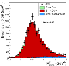
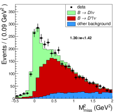
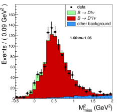
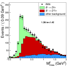
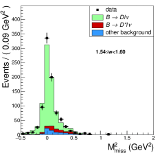
Figure 1: (Color online) Fit to the missing mass squared distribution in three bins of $w$ for the $B^{+}\to\bar{D}^{0}e^{+}\nu_{e}$ sub-sample. Points with error bars are the data. Histograms are (from top to bottom) the $B\to D\ell\nu_{\ell}$ signal (green), the $B\to D^{*}\ell\nu_{\ell}$ cross-feed background (red), and other backgrounds (blue). The $p$-values of the fits are (from left to right) 0.55, 0.21, and 0.10.

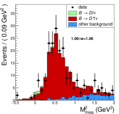
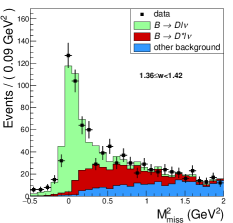
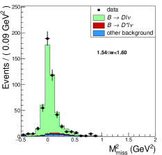
Figure 2: Same as Fig. 4 for the $B^{+}\to\bar{D}^{0}\mu^{+}\nu_{\mu}$ sub-sample. The $p$-values of the fits are (from left to right) 0.71, 0.38, and 0.42.

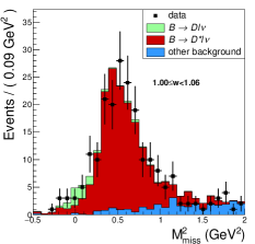
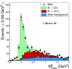
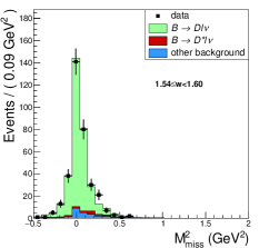
Figure 3: Same as Fig. 4 for the $B^{0}\to D^{-}e^{+}\nu_{e}$ sub-sample. The $p$-values of the fits are (from left to right) 0.30, 0.10, and 0.96.

Figure 4: Same as Fig. 4 for the $B^{0}\to D^{-}\mu^{+}\nu_{\mu}$ sub-sample. The $p$-values of the fits are (from left to right) 0.92, 0.39, and 1.00.

III Results and Systematic Uncertainties

III.1 Results

In each of the 4 sub-samples, we determine the differential decay width as a function of $w$ using

$$\frac{\Delta\Gamma_{i}}{\Delta w}=\frac{\Delta\Gamma_{i,\mathrm{MC}}}{\Delta w}\frac{\tau_{\mathrm{MC}}}{\tau}\frac{N_{i}}{N_{i,\mathrm{MC}}}~{},\quad i=0,\dots,9\,.$$ (15)

Here, $\Delta\Gamma_{i,\mathrm{MC}}/\Delta w$ is the differential $B\to D\ell\nu_{\ell}$ width expected in the $i^{\mathrm{th}}$ bin of $w$ assuming the values of the CLN parameters used in the MC:

$$\frac{\Delta\Gamma_{i,\mathrm{MC}}}{\Delta w}=\frac{1}{\Delta w}\int_{w_{i,\mathrm{min}}}^{w_{i,\mathrm{max}}}\frac{d\Gamma_{\mathrm{CLN}}}{dw}dw~{},$$ (16)

where $w_{i,\mathrm{min}}$ and $w_{i,\mathrm{max}}$ are the boundaries of the $i^{\mathrm{th}}$ bin. Depending on the sub-sample, $\tau$ is the $B^{+}$ or $B^{0}$ lifetime ($\tau_{B^{0}}=1.519$ ps and $\tau_{B^{+}}=1.638$ ps, respectively Agashe:2014kda ) and $\tau_{\mathrm{MC}}$ is the corresponding quantity in the MC simulation. Finally, $N_{i}$ is the $B\to D\ell\nu_{\ell}$ signal yield measured by the missing-mass-squared fit in the $i^{\mathrm{th}}$ bin of $w$, and $N_{i,\mathrm{MC}}$ is the same quantity in the MC simulation after scaling to the data luminosity and applying all corrections mentioned in Sect. II.1.

The results of $\Delta\Gamma_{i}/\Delta w$ for the sub-samples $B^{+}\to\bar{D}^{0}e^{+}\nu_{e}$, $B^{+}\to\bar{D}^{0}\mu^{+}\nu_{\mu}$, $B^{0}\to D^{-}e^{+}\nu_{e}$, and $B^{0}\to D^{-}\mu^{+}\nu_{\mu}$ are shown in Table 1 and show very good consistency. The full correlation matrix of the systematic errors in different $w$-bins in the sub-sample results are determined with the approach described in Sect. III.2 and can be found in Ref. epaps . The weighted average of the differential rates is calculated by taking into account the full experimental correlations of all four individual measurements. The resulting central values, uncertainties and correlations are summarized in Table 2. Similarly, we calculate the branching fractions of the decays $B^{+}\to\bar{D}^{0}e^{+}\nu_{e}$, $B^{+}\to\bar{D}^{0}\mu^{+}\nu_{\mu}$, $B^{0}\to D^{-}e^{+}\nu_{e}$, and $B^{0}\to D^{-}\mu^{+}\nu_{\mu}$ from the measured differential widths using the expression

$$\mathcal{B}=\tau_{B}\sum\limits_{i}\Delta\Gamma_{i}~{}.$$ (17)

Here, $\tau_{B}$ is the corresponding $B$ meson lifetime and $\Delta\Gamma_{i}$ are the measured values of $\Delta\Gamma_{i}/\Delta w$ times the $\Delta w$ used in the $i^{\mathrm{th}}$ bin. The results are quoted in Table 3. We also quote combined results for charged and neutral $B$ meson decays and for all four sub-samples combined. The ratio $R_{D}^{\mu/e}=\mathcal{B}(B\to D\mu\nu)/\mathcal{B}(B\to De\nu)$ is found to be $0.995\pm 0.022(\mathrm{stat})\pm 0.039(\mathrm{syst})$.

Table 1: The values of $\Delta\Gamma_{i}/\Delta w$ with the statistical and systematic uncertainties in the $B^{+}\to\bar{D}^{0}e^{+}\nu_{e}$, $B^{+}\to\bar{D}^{0}\mu^{+}\nu_{\mu}$, $B^{0}\to D^{-}e^{+}\nu_{e}$, and $B^{0}\to D^{-}\mu^{+}\nu_{\mu}$ sub-samples. $i$, $w_{i,\mathrm{min}}$ and $w_{i,\mathrm{max}}$ are the $w$-bin number, lower and upper edge of the bin respectively. The value of $w_{\mathrm{max}}$ is 1.59209 for the sub-samples with a charged $B$ meson and 1.58901 for the sub-samples with a neutral $B$ meson. The $\Delta\Gamma_{i}/\Delta w$ results are statistically uncorrelated amongst bins and samples. The systematic correlations between bins and samples are given in Ref. epaps .

			$\Delta\Gamma_{i}/\Delta w$[$10^{-15}$GeV]
$i$	$w_{i,\mathrm{min}}$	$w_{i,\mathrm{max}}$	$B^{0}\to D^{-}e^{+}\nu_{e}$	$B^{0}\to D^{-}\mu^{+}\nu_{\mu}$	$B^{+}\to\bar{D}^{0}e^{+}\nu_{e}$	$B^{+}\to\bar{D}^{0}\mu^{+}\nu_{\mu}$
0	1.00	1.06	$0.30\pm 0.31\pm 0.06$	$0.81\pm 0.47\pm 0.07$	$0.72\pm 0.67\pm 0.12$	$1.33\pm 0.42\pm 0.09$
1	1.06	1.12	$4.41\pm 0.85\pm 0.22$	$3.63\pm 0.72\pm 0.17$	$3.84\pm 0.81\pm 0.24$	$4.28\pm 0.70\pm 0.24$
2	1.12	1.18	$9.06\pm 1.14\pm 0.44$	$7.73\pm 1.04\pm 0.37$	$7.64\pm 0.90\pm 0.41$	$7.52\pm 0.92\pm 0.41$
3	1.18	1.24	$11.81\pm 1.28\pm 0.58$	$13.47\pm 1.42\pm 0.67$	$11.20\pm 1.01\pm 0.61$	$11.76\pm 0.97\pm 0.62$
4	1.24	1.30	$13.73\pm 1.35\pm 0.67$	$14.11\pm 1.42\pm 0.70$	$14.68\pm 1.11\pm 0.80$	$17.54\pm 1.18\pm 0.93$
5	1.30	1.36	$19.92\pm 1.51\pm 0.97$	$20.09\pm 1.59\pm 0.98$	$20.15\pm 1.15\pm 1.06$	$20.67\pm 1.20\pm 1.08$
6	1.36	1.42	$25.45\pm 1.70\pm 1.26$	$24.63\pm 1.73\pm 1.21$	$24.20\pm 1.22\pm 1.25$	$24.45\pm 1.28\pm 1.27$
7	1.42	1.48	$30.45\pm 1.78\pm 1.47$	$29.48\pm 1.85\pm 1.42$	$28.92\pm 1.25\pm 1.50$	$26.93\pm 1.28\pm 1.39$
8	1.48	1.54	$31.57\pm 1.73\pm 1.50$	$30.31\pm 1.93\pm 1.46$	$30.90\pm 1.22\pm 1.57$	$29.85\pm 1.36\pm 1.50$
9	1.54	$w_{\mathrm{max}}$	$35.81\pm 1.88\pm 1.68$	$34.62\pm 2.19\pm 1.63$	$34.42\pm 1.24\pm 1.73$	$32.83\pm 1.44\pm 1.63$

Table 2: The values of $\Delta\Gamma_{i}/\Delta w$ obtained in different bins of $w$ after combination of the $B^{+}\to\bar{D}^{0}e^{+}\nu_{e}$, $B^{+}\to\bar{D}^{0}\mu^{+}\nu_{\mu}$, $B^{0}\to D^{-}e^{+}\nu_{e}$, and $B^{0}\to D^{-}\mu^{+}\nu_{\mu}$ sub-samples. The columns are (from left to right) the bin number, the lower and the upper edge of the $i^{\mathrm{th}}$ bin, the value of $\Delta\Gamma_{i}/\Delta w$ in this bin with the statistical and systematic uncertainties, and the correlation matrix of the systematic error. The value of $w_{\mathrm{max}}=1.59055$ is the average of the values for charged and neutral $B$ mesons.

				$\rho_{ij,\mathrm{syst}}$
$i$	$w_{i,\mathrm{min}}$	$w_{i,\mathrm{max}}$	$\Delta\Gamma_{i}/\Delta w$[$10^{-15}$GeV]	0	1	2	3	4	5	6	7	8	9
0	1.00	1.06	$0.68\pm 0.21\pm 0.05$	1.000	0.682	0.677	0.663	0.654	0.656	0.664	0.648	0.608	0.560
1	1.06	1.12	$3.88\pm 0.38\pm 0.18$		1.000	0.976	0.974	0.969	0.972	0.972	0.961	0.933	0.900
2	1.12	1.18	$7.59\pm 0.50\pm 0.35$			1.000	0.991	0.987	0.990	0.989	0.980	0.959	0.929
3	1.18	1.24	$11.42\pm 0.58\pm 0.54$				1.000	0.993	0.993	0.990	0.980	0.961	0.934
4	1.24	1.30	$14.59\pm 0.64\pm 0.69$					1.000	0.996	0.992	0.985	0.972	0.952
5	1.30	1.36	$19.49\pm 0.69\pm 0.91$						1.000	0.996	0.991	0.979	0.956
6	1.36	1.42	$23.66\pm 0.76\pm 1.10$							1.000	0.995	0.981	0.952
7	1.42	1.48	$27.56\pm 0.79\pm 1.27$								1.000	0.992	0.968
8	1.48	1.54	$29.52\pm 0.80\pm 1.34$									1.000	0.985
9	1.54	$w_{\mathrm{max}}$	$33.37\pm 0.86\pm 1.50$										1.000

Table 3: Branching fractions of the decays $B^{+}\to\bar{D}^{0}e^{+}\nu_{e}$, $B^{+}\to\bar{D}^{0}\mu^{+}\nu_{\mu}$, $B^{0}\to D^{-}e^{+}\nu_{e}$, and $B^{0}\to D^{-}\mu^{+}\nu_{\mu}$. The branching fractions of $B^{+}\to\bar{D}^{0}\ell^{+}\nu_{\ell}$ ($B^{0}\to D^{-}\ell^{+}\nu_{\ell}$) are the weighted averages of the $B^{+}\to\bar{D}^{0}e^{+}\nu_{e}$ and $B^{+}\to\bar{D}^{0}\mu^{+}\nu_{\mu}$ ($B^{0}\to D^{-}e^{+}\nu_{e}$ and $B^{0}\to D^{-}\mu^{+}\nu_{\mu}$) branching fraction results. The last row of the table corresponds to the branching fraction of all four sub-samples combined, expressed in terms of the neutral mode $B^{0}\to D^{-}\ell^{+}\nu_{\ell}$ assuming the lifetime $\tau_{B^{0}}=1.519$ Agashe:2014kda . The first error on the yields and on the branching fractions is statistical. The second uncertainty is systematic.

Sample	Signal yield	$\mathcal{B}$ [%]
$B^{0}\to D^{-}e^{+}\nu_{e}$	$2848\pm 72\pm 17$	$2.44\pm 0.06\pm 0.12$
$B^{0}\to D^{-}\mu^{+}\nu_{\mu}$	$2302\pm 63\pm 13$	$2.39\pm 0.06\pm 0.11$
$B^{+}\to\bar{D}^{0}e^{+}\nu_{e}$	$6456\pm 126\pm 66$	$2.57\pm 0.05\pm 0.13$
$B^{+}\to\bar{D}^{0}\mu^{+}\nu_{\mu}$	$5386\pm 110\pm 51$	$2.58\pm 0.05\pm 0.13$
$B^{0}\to D^{-}\ell^{+}\nu_{\ell}$	$5150\pm 95\pm 29$	$2.39\pm 0.04\pm 0.11$
$B^{+}\to\bar{D}^{0}\ell^{+}\nu_{\ell}$	$11843\pm 167\pm 120$	$2.54\pm 0.04\pm 0.13$
$B\to D\ell\nu_{\ell}$	$16992\pm 192\pm 142$	$2.31\pm 0.03\pm 0.11$

III.2 Systematic uncertainties

We use a toy MC approach to estimate systematic uncertainties of the values of $\Delta\Gamma_{i}/\Delta w$ and their correlations. For a given systematic error component, we vary one or several parameters in the MC simulation according to a Gaussian distribution with a width corresponding to the systematic uncertainty under study. This altered MC sample is then used to repeat the entire analysis procedure, resulting in an updated value of $\Delta\Gamma_{i}/\Delta w$. Repeating this procedure 1000 times, we obtain a distribution of $\Delta\Gamma_{i}/\Delta w$ values corresponding to this specific systematic error component. The distribution is fitted with a Gaussian function and the width $\sigma_{i}$ of the Gaussian function is taken as the estimate of the contribution of this error component to the total systematic uncertainty. The corresponding correlation $\rho_{i,j}$ between $\Delta\Gamma_{i}/\Delta w$ and $\Delta\Gamma_{j}/\Delta w$ is calculated as

$$\rho_{i,j}=\frac{\langle(\frac{\Delta\Gamma_{i}}{\Delta w}-\langle\frac{\Delta\Gamma_{i}}{\Delta w}\rangle)(\frac{\Delta\Gamma_{j}}{\Delta w}-\langle\frac{\Delta\Gamma_{j}}{\Delta w}\rangle)\rangle}{\sqrt{\langle(\frac{\Delta\Gamma_{i}}{\Delta w}-\langle\frac{\Delta\Gamma_{i}}{\Delta w}\rangle)^{2}\rangle}\sqrt{\langle(\frac{\Delta\Gamma_{j}}{\Delta w}-\langle\frac{\Delta\Gamma_{j}}{\Delta w}\rangle)^{2}\rangle}}~{},$$ (18)

where the average indicated by the brackets is taken over the toy MC sample. To reduce the effect of outliers, toy MC events where one value of $\Delta\Gamma_{i}/\Delta w$ lies outside of the interval $\pm 3\sigma_{i}$ are removed. The elements of the covariance matrix are then calculated as $\rho_{i,j}\sigma_{i}\sigma_{j}$. The full systematic error matrix is obtained by adding the covariance matrices corresponding to the individual error components linearly. This is equivalent to the quadratic addition of the systematic error components of $\Delta\Gamma_{i}/\Delta w$. The individual systematic error components are described in the following.

Tag correction: This error component is estimated in two steps: we apply all the corrections to the MC mentioned in Sect. II.1 and vary these within their respective uncertainties. This results in systematic uncertainties in the 480 tag correction coefficients introduced in Sect. II.2. Finally, we propagate the uncertainties in the tag correction coefficients to the values of $\Delta\Gamma_{i}/\Delta w$. The statistical uncertainties in the tag corrections are varied independently while the systematic errors on the coefficients are conservatively assumed to be 100% correlated.

Charged track reconstruction: We assume a 0.35% reconstruction uncertainty for each charged particle in the final state. This uncertainty is added linearly for each charged particle on the signal side, as the charged particle reconstruction on the tag side is already corrected by our tag calibration. This uncertainty is propagated to $\Delta\Gamma_{i}/\Delta w$ using the toy MC approach.

Branching fractions and form factors (FF): We adjust the branching fraction and the CLN form factor of the decay $B\to D^{*}\ell\nu_{\ell}$ – the main cross-feed background – in the MC Agashe:2014kda ; HFAG_averages . Also, for semileptonic decays to orbitally excited $D$ meson states $B\to D^{**}\ell\nu_{\ell}$, we correct both the rate and the form factor Agashe:2014kda ; leibovich1998semileptonic . For the $D$ meson decays, only the branching fractions are adjusted Agashe:2014kda . The error component corresponding to charmless semileptonic decays $B\to X_{u}\ell\nu_{\ell}$ contains both the uncertainty in the inclusive $b\to u\ell\nu$ rate HFAG_averages and in the known exclusive decays ($B\to\pi\ell\nu,\rho\ell\nu,\omega\ell\nu,\eta\ell\nu,\eta^{\prime}\ell\nu$) Agashe:2014kda .

Signal shape: This error component corresponds to the uncertainty in the smearing parameter of the signal shape correction described in Sect. II.4.

$B$ lifetime: The lifetimes of $B^{0}$ and $B^{+}$ are needed in Eq. (15) to determine $\Delta\Gamma_{i}/\Delta w$. We use the following central values and uncertainties: $\tau(B^{0})=1.519\pm 0.005$ ps and $\tau(B^{+})=1.638\pm 0.004$ ps Agashe:2014kda .

Particle identification: Due to the use of the tag calibration sample, the uncertainty in the charged lepton identification cancels. A remaining particle-identification uncertainty arises from kaon and pion identification, which is estimated using a data sample of $D^{*+}\to D^{0}\pi^{+}$ decays. The misidentification probability of pions as electrons or as muons is also adjusted in MC simulation by using real $D^{*+}\to D^{0}\pi^{+}$ events.

Luminosity: This component includes the uncertainty in the measurement of the Belle data luminosity (1.4%) and the uncertainty in the branching fraction of $\Upsilon(4S)\to B\bar{B}$ Agashe:2014kda . The luminosity measurement uses Bhabha events and its uncertainty is dominated by the accuracy of the event generator used.

The systematic uncertainties in $\Delta\Gamma_{i}/\Delta w$ are itemized in Table 4. Since signal is suppressed at zero recoil, the zeroth bin has the largest relative uncertainty. The systematic uncertainties of the branching fractions in Table 3 are estimated by using the same toy MC approach and the same error components.

Table 4: Itemization of the systematic uncertainty in $\Delta\Gamma_{i}/\Delta w$ in each $w$ bin. Refer to the main text for more details on the systematic error components.

	$\sigma\left(\Delta\Gamma_{i}/\Delta w\right)$[%]
	0	1	2	3	4	5	6	7	8	9
Tag correction	3.0	3.2	3.3	3.4	3.4	3.4	3.4	3.3	3.3	3.2
Charged tracks	1.7	1.6	1.6	1.6	1.6	1.6	1.6	1.6	1.6	1.6
$\mathcal{B}(D\to$ hadronic $)$	2.0	1.8	1.8	1.8	1.8	1.8	1.8	1.9	1.9	1.9
$\mathcal{B}(B\to D^{*(*)}\ell\nu)$	1.3	0.8	0.8	0.9	0.8	0.7	0.5	0.2	0.2	0.4
$\mathcal{B}(B\to X_{u}\ell\nu)$	0.4	0.1	0.0	0.1	0.0	0.0	0.0	0.0	0.0	0.0
FF($B\to D^{*}\ell\nu$)	0.4	0.2	0.2	0.2	0.2	0.1	0.1	0.1	0.1	0.2
FF($B\to D^{**}\ell\nu$)	2.5	1.2	0.9	0.7	0.5	0.5	0.7	0.5	0.1	0.4
Signal shape	5.0	0.8	0.6	0.5	0.5	0.4	0.3	0.3	0.2	0.1
Lifetimes	0.2	0.2	0.2	0.2	0.2	0.2	0.2	0.2	0.2	0.2
$\pi^{0}$ efficiency	0.9	0.6	0.6	0.6	0.6	0.6	0.6	0.6	0.6	0.7
$K/\pi$ efficiency	1.1	0.9	0.9	0.9	0.9	0.9	0.9	1.0	1.0	1.0
$K_{S}$ efficiency	0.4	0.2	0.2	0.2	0.2	0.2	0.2	0.2	0.2	0.2
Luminosity	1.4	1.4	1.5	1.4	1.4	1.4	1.4	1.4	1.4	1.4
Total	7.3	4.7	4.7	4.7	4.7	4.6	4.7	4.6	4.5	4.5

IV Discussion

IV.1 CLN parameterization interpretation

The usual approach used in the literature HFAG_averages to interpret the $\Delta\Gamma/\Delta w$ distribution is to perform a fit to the CLN form-factor parameterization (Eq. 13), determine $\eta_{\mathrm{EW}}\mathcal{G}(1)|V_{cb}|$ and obtain $\eta_{\mathrm{EW}}|V_{cb}|$ by dividing by $\mathcal{G}(1)$. We do so here and determine the overall normalization $\eta_{\mathrm{EW}}\mathcal{G}(1)|V_{cb}|$ and the parameter $\rho^{2}$ of the CLN form-factor parameterization by minimizing the $\chi^{2}$ function

$$\chi^{2}=\sum\limits_{i,j}(\frac{\Delta\Gamma_{i}}{\Delta w}-\frac{\Delta\Gamma_{i,\mathrm{CLN}}}{\Delta w})\mathbf{C}^{-1}_{ij}(\frac{\Delta\Gamma_{j}}{\Delta w}-\frac{\Delta\Gamma_{j,\mathrm{CLN}}}{\Delta w})~{},$$ (19)

where $\Delta\Gamma_{i}/\Delta w$ is the measured value from Table 1 or 2 and $\Delta\Gamma_{i,\mathrm{CLN}}/\Delta w$ is the partial width calculated using Eqs. 5 and 13:

$$\frac{\Delta\Gamma_{i,\mathrm{CLN}}}{\Delta w}(\eta_{\mathrm{EW}}\mathcal{G}(1)|V_{cb}|,\rho^{2})=\frac{1}{\Delta w}\int_{w_{i,\mathrm{min}}}^{w_{i,\mathrm{max}}}\frac{d\Gamma_{\mathrm{CLN}}}{dw}dw~{}.$$ (20)

The total covariance matrix $\mathbf{C}$ is the sum of the diagonal statistical error matrix $\mathbf{C}_{\mathrm{stat}}$ and the systematic covariance matrix $\mathbf{C}_{\mathrm{syst}}$, calculated from the systematic errors and correlations presented in Sect. III. For the fit on the combined sample we use the averaged nominal masses of charged and neutral mesons ($m_{B}=5.27942$ GeV and $m_{D}=1.86723$ GeV).

The result of the fit is shown in Fig. 5. The results in terms of $\eta_{\mathrm{EW}}\mathcal{G}(1)|V_{cb}|$ and $\rho^{2}$ are given in Table 5 and Fig. 6, separately for the $B^{+}\to\bar{D}^{0}e^{+}\nu_{e}$, $B^{+}\to\bar{D}^{0}\mu^{+}\nu_{\mu}$, $B^{0}\to D^{-}e^{+}\nu_{e}$, and $B^{0}\to D^{-}\mu^{+}\nu_{\mu}$ sub-samples and for the combined spectrum. Assuming the form-factor normalization $\mathcal{G}(1)$ derived in Ref. lattice2015b

$$\mathcal{G}(1)=1.0541\pm 0.0083~{},$$ (21)

we obtain $\eta_{\mathrm{EW}}|V_{cb}|=(40.12\pm 1.34)\times 10^{-3}$.

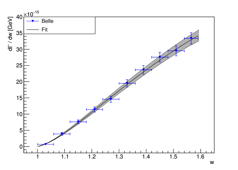
Figure 5: Fit to the measured $\Delta\Gamma/\Delta w$ spectrum of the decay $B\to D\ell\nu_{\ell}$, assuming the CLN form-factor parameterization (Eq. (13)). The points with error bars are the data. Their respective uncertainties are shown by the vertical error bars; the bin widths are shown by the horizontal bars. The solid curve corresponds to the result of the fit. The shaded area around this curve indicates the uncertainty in the coefficients of the CLN parameters.

Table 5: Result of the fit to the measured $\Delta\Gamma/\Delta w$ spectrum of the decay $B\to D\ell\nu_{\ell}$ using the CLN form-factor parameterization (Eq. (13)). The CLN parameters $\eta_{\mathrm{EW}}\mathcal{G}(1)|V_{cb}|$ and $\rho^{2}$ are given for the $B^{+}\to\bar{D}^{0}e^{+}\nu_{e}$, $B^{+}\to\bar{D}^{0}\mu^{+}\nu_{\mu}$, $B^{0}\to D^{-}e^{+}\nu_{e}$, and $B^{0}\to D^{-}\mu^{+}\nu_{\mu}$ sub-samples and for all four sub-samples combined (based on the combined sample shown in Table 2). The value of $\eta_{\mathrm{EW}}|V_{cb}|$ is obtained assuming the form-factor normalization in Eq. (21). “Correlation” denotes the measured correlation between the overall uncertainties of $\eta_{\mathrm{EW}}\mathcal{G}(1)|V_{cb}|$ and $\rho^{2}$.

	$B^{+}\to\bar{D}^{0}e^{+}\nu_{e}$	$B^{+}\to\bar{D}^{0}\mu^{+}\nu_{\mu}$	$B^{0}\to D^{-}e^{+}\nu_{e}$	$B^{0}\to D^{-}\mu^{+}\nu_{\mu}$	$B\to D\ell\nu_{\ell}$
$\eta_{\mathrm{EW}}\mathcal{G}(1)|V_{cb}|$[$10^{-3}$]	$42.31\pm 1.94$	$45.48\pm 1.96$	$41.84\pm 2.14$	$42.99\pm 2.18$	$42.29\pm 1.37$
$\rho^{2}$	$1.05\pm 0.08$	$1.22\pm 0.07$	$1.01\pm 0.10$	$1.08\pm 0.10$	$1.09\pm 0.05$
Correlation	$0.81$	$0.77$	$0.85$	$0.84$	$0.69$
$\eta_{\mathrm{EW}}|V_{cb}|$[$10^{-3}$]	$40.14\pm 1.86$	$43.15\pm 1.89$	$39.69\pm 2.05$	$40.78\pm 2.09$	$40.12\pm 1.34$
$\chi^{2}/n_{\mathrm{df}}$	$2.19/8$	$2.71/8$	$9.65/8$	$4.36/8$	$4.57/8$
Prob.	$0.97$	$0.95$	$0.29$	$0.82$	$0.80$

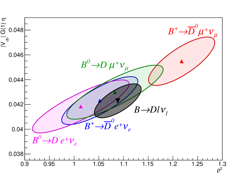
Figure 6: Result of the fit assuming the CLN form-factor parameterization (Eq. (13)). The error ellipses ($\Delta\chi^{2}=1$) of $\eta_{\mathrm{EW}}\mathcal{G}(1)|V_{cb}|$ and $\rho^{2}$ are shown for the fit to the $B^{+}\to\bar{D}^{0}e^{+}\nu_{e}$, $B^{+}\to\bar{D}^{0}\mu^{+}\nu_{\mu}$, $B^{0}\to D^{-}e^{+}\nu_{e}$, and $B^{0}\to D^{-}\mu^{+}\nu_{\mu}$ sub-samples, and to the combined sample.

IV.2 Model-independent BGL fit

Recent lattice data at non-zero recoil lattice2015b ; na2015b allows us to perform a combined fit to the BGL form factor. We proceed as in the previous section and minimize the $\chi^{2}$ function

$$\chi^{2}=\sum\limits_{i,j}(\frac{\Delta\Gamma_{i}}{\Delta w}-\frac{\Delta\Gamma_{i,\mathrm{BGL}}}{\Delta w})\mathbf{C}^{-1}_{ij}(\frac{\Delta\Gamma_{j}}{\Delta w}-\frac{\Delta\Gamma_{j,\mathrm{BGL}}}{\Delta w})+\sum\limits_{k,l}\left(f^{\mathrm{LQCD}}_{+,0}(w_{k})-f^{\mathrm{BGL}}_{+,0}(w_{k})\right)\mathbf{D}^{-1}_{kl}\left((f^{\mathrm{LQCD}}_{+,0}(w_{l})-f^{\mathrm{BGL}}_{+,0}(w_{l})\right)~{}.$$ (22)

Again, $\Delta\Gamma_{i}/\Delta w$ is taken from Table 2 and $\Delta\Gamma_{i,\mathrm{BGL}}/\Delta w$ is the partial width calculated using Eqs. 5, 6, and 8

$$\frac{\Delta\Gamma_{i,\mathrm{BGL}}}{\Delta w}(\eta_{\mathrm{EW}}|V_{cb}|,a_{+,n})=\frac{1}{\Delta w}\int_{w_{i,\mathrm{min}}}^{w_{i,\mathrm{max}}}\frac{d\Gamma_{\mathrm{BGL}}}{dw}dw~{}.$$ (23)

The error matrix $\mathbf{C}$ includes the statistical and systematic uncertainties in the measurements of $\Delta\Gamma_{i}/\Delta w$. The data is fit together with predictions of lattice QCD (LQCD), which are available for the form factors $f_{+}(w)$ and $f_{0}(w)$ at selected points in $w$. The second sum runs over all LQCD predictions included in the fit and the corresponding error matrix $\mathbf{D}$ contains the LQCD uncertainty in these predictions. We use lattice data obtained by the FNAL/MILC and HPQCD collaborations lattice2015b ; na2015b . Both LQCD calculations are dominated by their systematic errors. The correlation between them is expected to be small since the collaborations use different heavy-quark methods, lattice NRQCD Lepage:1992tx for HPQCD and the Fermilab method ElKhadra:1996mp for FNAL/MILC. We therefore assume the two LQCD results to be uncorrelated in our fits.

Note that LQCD yields results for both the $f_{+}$ and $f_{0}$ form factors while the experimental distribution $\Delta\Gamma_{i}/\Delta w$ depends on $f_{+}$ only. Using the kinematic constraint from Eq. 7, we can include the LQCD results for $f_{0}$ into the fit, allowing us to better constrain $f_{+}$. Following Ref. lattice2015b , we implement this constraint by expressing $a_{0,0}$ in terms of the other $a_{+,n}$ and $a_{0,n}$ coefficients. FNAL/MILC obtains values for both the $f_{+}$ and the $f_{0}$ form factors at $w$ values of 1, 1.08, and 1.16. The full covariance matrix for these six measurements is available in Table VII of Ref. lattice2015b .

The form factors determined by HPQCD are based on a different form factor parameterization by Bourrely, Caprini and Lellouch (BCL), see Ref. BCL . BCL uses an expansion in a conformal mapping variable to offer perturbative QCD scaling also at higher $q^{2}$ values. The formulae and pole choices used by HPQCD can be seen in Eqs. A1 to A6 of Ref. na2015b . As a result of their fit they provide the coefficients $a^{(0)}_{0}$, $a^{(0)}_{1}$, $a^{(0)}_{2}$, $a^{(+)}_{0}$, $a^{(+)}_{1}$, and $a^{(+)}_{2}$, together with their $6\times 6$ covariance matrix (Table VII of Ref. na2015b ). To be able to include these results in the same fit as the FNAL/MILC points, we transform the coefficients into the form-factor values of $f_{+}$ and $f_{0}$ at $w=1,1.08$ and $1.16$:

$$\left(\begin{array}[]{c}f_{0}(1)\\ f_{0}(1.08)\\ f_{0}(1.16)\\ f_{+}(1)\\ f_{+}(1.08)\\ f_{+}(1.16)\end{array}\right)=\mathbf{M}\left(\begin{array}[]{c}a^{(0)}_{0}\\ a^{(0)}_{1}\\ a^{(0)}_{2}\\ a^{(+)}_{0}\\ a^{(+)}_{1}\\ a^{(+)}_{2}\end{array}\right)~{},$$ (24)

where $\mathbf{M}$ is a block-diagonal $6\times 6$ matrix. Denoting the covariance matrix of the HPQCD $a$-parameters by $\mathbf{Cov}(a)$, the error matrix of the form-factor values becomes $\mathbf{M}~{}\mathbf{Cov}(a)~{}\mathbf{M}^{T}$. The HPQCD results in terms of the $f_{+}$ and $f_{0}$ form factors at $w=1,1.08$ and $1.16$, together with their correlation coefficients, are given in Table 6.

Table 6: Lattice QCD results obtained by the HPQCD collaboration na2015b , expressed in terms of $f_{+}$ and $f_{0}$ form-factor values at $w=1,1.08$ and $1.16$.

		Correlation coefficients
	Central value	$f_{+}(1)$	$f_{+}(1.08)$	$f_{+}(1.16)$	$f_{0}(1)$	$f_{0}(1.08)$	$f_{0}(1.16)$
$f_{+}(1)$	$1.178\pm 0.046$	1.000	0.989	0.954	0.507	0.518	0.525
$f_{+}(1.08)$	$1.082\pm 0.041$		1.000	0.988	0.582	0.600	0.615
$f_{+}(1.16)$	$0.996\pm 0.037$			1.000	0.650	0.676	0.698
$f_{0}(1)$	$0.902\pm 0.041$				1.000	0.995	0.980
$f_{0}(1.08)$	$0.860\pm 0.038$					1.000	0.995
$f_{0}(1.16)$	$0.821\pm 0.036$						1.000

Table 7 shows the result of the BGL fit to experimental and LQCD data (FNAL/MILC and HPQCD) for different truncation orders of the series ($N=2,3,4$). To implement the unitarity bound (Eq. (12)), we constrain the cubic and quartic coefficients in Eq. (8) to $0\pm 1$ in the fits with $N=3$ and $N=4$ by adding measurement points of $a_{+,i\geq 3}$ and $a_{0,i\geq 3}$ to the $\chi^{2}$. This follows the method in Ref. lattice2015b and results in a constant number of degrees of freedom. For $N\geq 3$, the fit stabilizes and we get a reasonable goodness of fit. We thus choose this truncation order as our preferred fit. The fit result in terms of $\Delta\Gamma/\Delta w$ and $f_{+,0}$ is shown for $N=3$ in Figs. 7 and 8, respectively. Our baseline result for $\eta_{\mathrm{EW}}|V_{cb}|$ for the combined fit to experimental and lattice QCD data is thus $(41.10\pm 1.14)\times 10^{-3}$. This is slightly more precise than the fit result using the CLN form-factor parameterization (2.8% vs. 3.3%) due to the additional input from LQCD. The additional lattice points are also the dominant cause of differences in the resulting values. We have verified the stability of this $\eta_{\mathrm{EW}}|V_{cb}|$ value by repeating the fit with different sets of lattice QCD data (Table 8) and the differences between the results are well below one standard deviation.

Table 7: Result of the combined fit to experimental and lattice QCD (FNAL/MILC and HPQCD) data for different truncation orders of the BGL series (Eq. (8)). Note that the value of $a_{0,0}$ is not determined from the fit but rather inferred using the kinematic constraint (Eq. (7)).

	$N=2$	$N=3$	$N=4$
$a_{+,0}$	0.0127 $\pm$ 0.0001	0.0126 $\pm$ 0.0001	0.0126 $\pm$ 0.0001
$a_{+,1}$	-0.091 $\pm$ 0.002	-0.094 $\pm$ 0.003	-0.094 $\pm$ 0.003
$a_{+,2}$	0.34 $\pm$ 0.03	0.34 $\pm$ 0.04	0.34 $\pm$ 0.04
$a_{+,3}$	–	-0.1 $\pm$ 0.6	-0.1 $\pm$ 0.6
$a_{+,4}$	–	–	0.0 $\pm$ 1.0
$a_{0,0}$	0.0115 $\pm$ 0.0001	0.0115 $\pm$ 0.0001	0.0115 $\pm$ 0.0001
$a_{0,1}$	-0.058 $\pm$ 0.002	-0.057 $\pm$ 0.002	-0.057 $\pm$ 0.002
$a_{0,2}$	0.22 $\pm$ 0.02	0.12 $\pm$ 0.04	0.12 $\pm$ 0.04
$a_{0,3}$	–	0.4 $\pm$ 0.7	0.4 $\pm$ 0.7
$a_{0,4}$	–	–	0.0 $\pm$ 1.0
$\eta_{\mathrm{EW}}|V_{cb}|$	40.01 $\pm$ 1.08	41.10 $\pm$ 1.14	41.10 $\pm$ 1.14
$\chi^{2}/n_{\mathrm{df}}$	24.7/16	11.4/16	11.3/16
Prob.	0.075	0.787	0.787

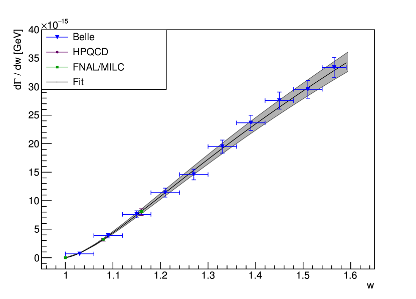
Figure 7: Differential width of ${B\to D\ell\nu_{\ell}}$ and result of the combined fit to experimental and lattice QCD (FNAL/MILC and HPQCD) data. The BGL series (Eq. (8)) is truncated after the cubic term. The points with error bars are Belle and LQCD data (only results for $f_{+}$ are shown on this plot). For Belle data, the uncertainties are represented by the vertical error bars and the bin widths by the horizontal bars. The solid curve corresponds to the result of the fit. The shaded area around this curve indicates the uncertainty in the coefficients of the BGL series.

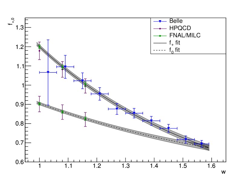
Figure 8: Form factors of the decay $B\to D\ell\nu_{\ell}$ and result of the combined fit to experimental and lattice QCD (FNAL/MILC and HPQCD) data. The BGL series (Eq. (8)) is truncated after the cubic term. The points with error bars are Belle and LQCD data. The solid curve is the $f_{+}$ form factor and the dashed curve represents $f_{0}$. The shaded areas around these curves indicate the uncertainty in the coefficients of the BGL expansion.

Table 8: Result of the combined fit to experimental data and different sets of lattice QCD data. The BGL series (Eq. (8)) is truncated after the cubic term.

Lattice data	$\eta_{\mathrm{EW}}|V_{cb}|$[$10^{-3}$]	$\chi^{2}/n_{\mathrm{df}}$	Prob.
FNAL/MILC lattice2015b	$40.96\pm 1.23$	6.01/10	0.81
HPQCD na2015b	$41.14\pm 1.88$	4.83/10	0.90
FNAL/MILC & HPQCD na2015b ; lattice2015b	$41.10\pm 1.14$	11.35/16	0.79

V Summary

We study the decay $B\to D\ell\nu_{\ell}$ in 711$\mbox{~{}fb}^{-1}$ of Belle $\Upsilon(4S)$ data and reconstruct about 5200 $B^{0}\to D^{-}\ell^{+}\nu_{\ell}$ and 11,800 $B^{+}\to\bar{D}^{0}\ell^{+}\nu_{\ell}$ decays. We determine the differential width $\Delta\Gamma/\Delta w$ of the decay as a function of the recoil variable $w=V_{B}\cdot V_{D}$.

The branching fractions of the decays $B^{+}\to\bar{D}^{0}e^{+}\nu_{e}$, $B^{+}\to\bar{D}^{0}\mu^{+}\nu_{\mu}$, $B^{0}\to D^{-}e^{+}\nu_{e}$, and $B^{0}\to D^{-}\mu^{+}\nu_{\mu}$ are obtained. The isospin-averaged branching fraction $\mathcal{B}(B^{0}\to D^{-}\ell^{+}\nu_{\ell})$ is determined to be $(2.31\pm 0.03(\mathrm{stat})\pm 0.11(\mathrm{syst}))\%$.

We interpret our measurement of $\Delta\Gamma/\Delta w$ in terms of $\eta_{\mathrm{EW}}|V_{cb}|$ by using the currently most established method, i.e., by fitting $\Delta\Gamma/\Delta w$ to the Caprini, Lellouch and Neubert (CLN) form-factor parameterization and by dividing $\eta_{\mathrm{EW}}\mathcal{G}(1)|V_{cb}|$ by the form factor normalization at zero recoil $\mathcal{G}(1)$ to obtain $\eta_{\mathrm{EW}}|V_{cb}|$. Assuming the value $\mathcal{G}(1)=1.0541\pm 0.0083$ lattice2015b , we find $\eta_{\mathrm{EW}}|V_{cb}|=(40.12\pm 1.34)\times 10^{-3}$. Recent lattice data also allows to perform a combined fit to the model-independent form-factor parameterization by Boyd, Grinstein and Lebed (BGL). We find $\eta_{\mathrm{EW}}|V_{cb}|=(41.10\pm 1.14)\times 10^{-3}$ with the lattice QCD data from FNAL/MILC lattice2015b and HPQCD na2015b .

Assuming $\eta_{\mathrm{EW}}=1.0066\pm 0.0016$ Sirlin1982 , our results correspond to a value of $|V_{cb}|=(39.86\pm 1.33)\times 10^{-3}$ for the fit using the CLN form-factor parameterization and $\mathcal{G}(1)$, and $|V_{cb}|=(40.83\pm 1.13)\times 10^{-3}$ for the fit using the BGL parameterization and lattice data.

These results supersede the previous Belle measurement Abe:2001yf . Compared to the previous analysis by BaBar Aubert:2009ac , we reconstruct about 5 times more $B\to D\ell\nu_{\ell}$ decays; this results in a significant improvement in the precision of the determination of $\eta_{\mathrm{EW}}|V_{cb}|$ from the decay $B\to D\ell\nu_{\ell}$ to 2.8%. The value of $\eta_{\mathrm{EW}}|V_{cb}|$ extracted with the combined analysis of experimental and LQCD data is in agreement with both $|V_{cb}|$ extracted from inclusive semileptonic decays Gambino_2013rza and $|V_{cb}|$ from $B\to D^{*}\ell\nu_{\ell}$ decays Dungel:2010uk ; Aubert:2007rs . The measured branching fractions are higher although still compatible with those obtained by previous analyses Aubert:2009ac .

VI Acknowledgments

We acknowledge useful discussions with Carleton DeTar, Daping Du, Andreas S. Kronfeld and Ruth Van de Water from the FNAL/MILC collaboration, and with Heechang Na and Junko Shigemitsu from HPQCD, as well as with Paolo Gambino and Florian Bernlochner, and the support of the Mainz Institute for Theoretical Physics.

We further thank the KEKB group for the excellent operation of the accelerator; the KEK cryogenics group for the efficient operation of the solenoid; and the KEK computer group, the National Institute of Informatics, and the PNNL/EMSL computing group for valuable computing and SINET4 network support. We acknowledge support from the Ministry of Education, Culture, Sports, Science, and Technology (MEXT) of Japan, the Japan Society for the Promotion of Science (JSPS), and the Tau-Lepton Physics Research Center of Nagoya University; the Australian Research Council; Austrian Science Fund under Grant No. P 22742-N16 and P 26794-N20; the National Natural Science Foundation of China under Contracts No. 10575109, No. 10775142, No. 10875115, No. 11175187, and No. 11475187; the Chinese Academy of Science Center for Excellence in Particle Physics; the Ministry of Education, Youth and Sports of the Czech Republic under Contract No. LG14034; the Carl Zeiss Foundation, the Deutsche Forschungsgemeinschaft and the VolkswagenStiftung; the Department of Science and Technology of India; the Istituto Nazionale di Fisica Nucleare of Italy; the WCU program of the Ministry of Education, National Research Foundation (NRF) of Korea Grants No. 2011-0029457, No. 2012-0008143, No. 2012R1A1A2008330, No. 2013R1A1A3007772, No. 2014R1A2A2A01005286, No. 2014R1A2A2A01002734, No. 2015R1A2A2A01003280 , No. 2015H1A2A1033649; the Basic Research Lab program under NRF Grant No. KRF-2011-0020333, Center for Korean J-PARC Users, No. NRF-2013K1A3A7A06056592; the Brain Korea 21-Plus program and Radiation Science Research Institute; the Polish Ministry of Science and Higher Education and the National Science Center; the Ministry of Education and Science of the Russian Federation and the Russian Foundation for Basic Research; the Slovenian Research Agency; the Basque Foundation for Science (IKERBASQUE) and the Euskal Herriko Unibertsitatea (UPV/EHU) under program UFI 11/55 (Spain); the Swiss National Science Foundation; the National Science Council and the Ministry of Education of Taiwan; and the U.S. Department of Energy and the National Science Foundation. This work is supported by a Grant-in-Aid from MEXT for Science Research in a Priority Area (“New Development of Flavor Physics”) and from JSPS for Creative Scientific Research (“Evolution of Tau-lepton Physics”).

References

(1)
N. Cabibbo, Phys. Rev. Lett. 10, 531 (1963).
(2)
M. Kobayashi and T. Maskawa, Prog. Theor. Phys. 49, 652 (1973).
(3)
P. Gambino and C. Schwanda, Phys. Rev. D 89, 014022 (2014), arXiv:1307.4551 [hep-ph].
(4)
W. Dungel et al. (Belle Collaboration), Phys. Rev. D 82, 112007 (2010), arXiv:1010.5620 [hep-ex].
(5)
B. Aubert et al. (BaBar Collaboration), Phys. Rev. D 77, 032002 (2008), arXiv:0705.4008 [hep-ex].
(6)
B. Aubert et al. (BaBar Collaboration), Phys. Rev. Lett. 104, 011802 (2010), arXiv:0904.4063 [hep-ex].
(7)
Y. Amhis et al. (Heavy Flavor Averaging Group (HFAG)), (2014), arXiv:1412.7515 [hep-ex].
(8)
In all formulae in this paper we set .
(9)
K. Olive et al. (Particle Data Group), Chin. Phys. C 38, 090001 (2014).
(10)
A. Bevan et al. (BaBar and Belle Collaborations), Eur. Phys. J. C 74, 3026 (2014), arXiv:1406.6311 [hep-ex].
(11)
M. Neubert, Phys. Lett. B 264, 455 (1991).
(12)
A. Sirlin, Nucl. Phys. B 196, 83 (1982).
(13)
I. Caprini, L. Lellouch, and M. Neubert, Nucl. Phys. B 530, 153 (1998).
(14)
C. G. Boyd, B. Grinstein, and R. F. Lebed, Phys. Rev. Lett. 74, 4603 (1995).
(15)
J. A. Bailey, A. Bazavov, C. Bernard, C. Bouchard, C. DeTar, D. Du, A. X. El-Khadra, J. Foley, E. D. Freeland, et al. (Fermilab Lattice and MILC Collaborations),
Phys. Rev. D 92, 034506 (2015), arXiv:1503.07237 [hep-lat].
(16)
S. Kurokawa and E. Kikutani, Nucl. Instrum. Methods Phys. Res. Sect.
A 499, 1 (2003), and other papers included in this Volume;
T. Abe et al., Prog. Theor. Exp. Phys. 2013, 03A001 (2013)
and references therein.
(17)
K. Hanagaki, H. Kakuno, H. Ikeda, T. Iijima, and T. Tsukamoto, Nucl. Instr. and Meth. A 485, 490 (2002).
(18)
A. Abashian et al., Nucl. Instr. and Meth. A 491, 69 (2002).
(19)
A. Abashian et al. (Belle Collaboration), Nucl. Instrum. Methods
Phys. Res. Sect. A 479, 117 (2002); also see detector section in
J.Brodzicka et al., Prog. Theor. Exp. Phys. 2012, 04D001 (2012).
(20)
D. J. Lange, Nucl. Instr. and Meth. A 462, 152 (2001).
(21)
R. Brun et al., GEANT 3.21, Report No, Tech. Rep. (CERN DD/EE/84-1, 1984).
(22)
E. Barberio and Z. Waş, Comput. Phys. Commun. 79, 291 (1994).
(23)
A. K. Leibovich, Z. Ligeti, I. W. Stewart, and M. B. Wise, Phys. Rev. D 57, 308 (1998).
(24)
K. Abe et al., Phys. Rev. D 64, 072001 (2001).
(25)
G. C. Fox and S. Wolfram, Phys. Rev. Lett. 41, 1581 (1978).
(26)M. Feindt, F. Keller, M. Kreps, T. Kuhr, S. Neubauer, D. Zander, and A. Zupanc, Nucl. Instr. and Meth. A 654, 432 (2011).
(27)
Charge-conjugate decays are implied throughout this analysis.
(28)
M. Feindt and U. Kerzel, Nucl. Instr. and Meth. A 559, 190 (2006).
(29)
A. Sibidanov et al. (Belle Collaboration), Phys. Rev. D 88, 032005 (2013), arXiv:1306.2781 [hep-ex].
(30)
R. Barlow and C. Beeston, Comput. Phys. Commun. 77, 219 (1993).
(31)
See supplemental material file SubsampleResults.csv in arXiv source files for a table of the measured differential decay widths in the sub-samples and their
full systematic correlation matrix.
(32)
H. Na, C. M. Bouchard, G. P. Lepage, C. Monahan, and J. Shigemitsu (HPQCD Collaboration), Phys. Rev. D 92 054510 (2015), arXiv:1505.03925 [hep-lat].
(33)
G. P. Lepage, L. Magnea, C. Nakhleh, U. Magnea and K. Hornbostel, Phys. Rev. D 46 4052 (1992), arXiv:hep-lat/9205007.
(34)
A. X. El-Khadra, A. S. Kronfeld and P. B. Mackenzie, Phys. Rev. D 55 3933 (1997), arXiv:hep-lat/9604004.
(35)
C. Bourrely, L. Lellouch, and I. Caprini, Phys. Rev. D 79 013008 (2009), arXiv:0807.2722 [hep-ph].
(36)
K. Abe, et al. (Belle Collaboration), Phys. Lett. B 526, 258 (2002), arXiv:hep-ex/0111082.