Exact finite reduced density matrix and von Neumann entropy for the Calogero model

Abstract

The information content of continuous quantum variables systems is usually studied using a number of well known approximation methods. The approximations are made to obtain the spectrum, eigenfunctions or the reduced density matrices that are essential to calculate the entropy-like quantities that quantify the information. Even in the sparse cases where the spectrum and eigenfunctions are exactly known the entanglement spectrum, i.e. the spectrum of the reduced density matrices that characterize the problem, must be obtained in an approximate fashion. In this work, we obtain analytically a finite representation of the reduced density matrices of the fundamental state of the N-particle Calogero model for a discrete set of values of the interaction parameter. As a consequence, the exact entanglement spectrum and von Neumann entropy is worked out.

I Introduction

During the last few years, there has been an increasing interest in the entanglement or, more generally, the information content of quantum states of systems with continuous quantum variables (CV) Chiribella2014 ; Braunstein2005 ; Cerf2007 ; Tichy2011 . This ample category basically comprises, but is not exhausted by, electrons in atomic or molecular systems and few particle model systems as the Moshinsky model Moshinsky1968 and the Calogero model Calogero1969 . For an early example of the application of information ideas to the internal continuous variables of an artificial atom see the work of Amovilli and March Amovilli2004 .

In this context, the amount of attention dedicated to the Moshinsky and, to a lesser extent, the Calogero models seems at odds with their importance or the consequences that their study could have in understanding more realistic systems. A casual onlooker would think so, but a more experienced one would remember the scarcity of exact results about CV systems and think otherwise. After all, the study of entanglement in spin systems did not reach its maturity until the exact formula to calculate the entanglement of formation of an arbitrary state of two qubits was obtained by Wootters Wootters1998 . This formula, together with the battery of many-body exactly solvable models is the cornerstone of the amazing development of the studies of entanglement in systems with finite Hilbert spaces Amico2008 . In particular, the development of approximate methods has benefited from the accumulation of benchmarks where they can be tested.

Incidentally, when the entanglement or information content of a quantum state is under study, it is calculated using a plethora of entropy-like functions Vedral2002 ; Nielsen2000 . Regrettably, the use of one or other is often dictated by what it is feasible to calculate for a given system and not by the requirements of some information task like it is mostly the case in spin systems, where the entanglement of formation, the distillable entanglement Bennett1996 ; Horodecki1998 ; Horodecki2001 and others come to mind. In the same sense, the entanglement of formation of Gaussian states, that are a genuine continuous variable system, can be determined Giedke2003 . Anyway, the use of the von Neumann entropy and the Jozsa-Robb-Wootters sub-entropy Jozsa1994 in CV systems is supported by rigorous arguments Nichols2003 rather than numerical evidence from particular systems. More recently, Iemini and Vianna Iemini2013 , have discussed how to compute the entanglement of indistinguishable particles pure states, both bosons and fermions, using the von Neumann entropy. On the other hand, in the work of Killoran et al Killoran2014 it is argued that any entanglement, even the one that appears amongst identical particles due to symmetrization can be extracted and used for some task. All in all, the case for studying the von Neumann entropy for systems of identical particles is stronger than ever.

The technical difficulties associated to the calculation of informational quantities in atomic-like systems have been discussed numerous times and roughly speaking they can be classified in two kinds. The first kind is related to the method employed to obtain the (approximate) quantum state and the second kind is related to what informational quantities can be effectively calculated from the quantum state, as has been said above. If the state is obtained using a finite Hamiltonian approximation, like the ones that result from the Hartree-Fock or the variational Ritz methods, there is no guarantee that it will be manageable enough to obtain the reduced density matrices that are necessary to calculate some entropy-like quantity, or that the approximate quantum state even resembles the exact one or its entanglement content. From an historical point of view it is interesting to note that this subject was the motivation that led Moshinsky to study the model that is now called so after him. Nevertheless, there has been a lot of progress in the study of CV systems from more measures to quantify the information, as the geometric entanglement Gottlieb2005 or the relative von Neumann entropy Byczuk2012 , to understand how the entanglement behaves when approximate solutions obtained with the Hartree-Fock method Zhang2014 or the Ritz method Osenda2007 ; Ferron2009 ; Pont2010 are analyzed, and the relationship between entanglement and energy in two-electron systems Majtey2012 .

Despite that the Moshinsky and Calogero models have exact solutions, allowing to obtain some of the required quantities to study the information content of their quantum states, most studies about both models are restricted to the so-called linear entropy, since it does not require a detailed knowledge of the reduced density matrix spectrum, as is the case for the von Neumann entropy. If the model considered has $N$ particles, then the $p$-particle reduced density matrix ($p$-RDM) can be obtained by tracing out $N-p$ particles from the density matrix of the whole system. Each of $p$-RDM can be used to obtain entropy-like quantities. The $p$-RDM has been obtained analytically for the N-particle Moshinsky system at arbitrary values of the interaction parameter Pruski72 . In ko13 the exact occupation numbers and the exact expression for the von Neumann p-entropies have been derived and their dependence on the interaction strength and the number of particles has been discussed. In this work we obtain an exact finite analytical expression for the $p$-RDM for the $N$-particle one-dimensional Calogero model. We explicitly compute the cases for $p=1$ and $N$ up to $5$ for the totally symmetric (bosonic) ground state wave function. We analyze this case thoroughly, while the analysis of a totally anti-symmetric (fermionic) ground state function is restricted to the simplest case, i.e. two particles and their 1-RDM, since it proceeds similarly to the symmetric one. As we will show, in each case the entanglement spectrum Li2008 ; Calabrese2008 is given by a finite number of eigenvalues if the coefficient that characterizes the interaction between the particles assumes certain particular values. We analyze the relationship between our results with those found for the Crandall and Hooke atoms for $N=2$ Manzano2010 and for the N-particle Moshinsky model ko13 ; Schilling ; Benavides .

II The model

We adopt for the $N$-particle Calogero Hamiltonian Calogero1969 the expression of Sutherland s71

$$H=\sum_{i=1}^{N}\,h(i)+\nu(\nu-1)\,\sum_{i<j}\,\frac{1}{(x_{i}-x_{j})^{2}}\,,$$ (1)

where

$$h(i)=\frac{1}{2}\,p_{i}^{2}+\frac{1}{2}\,\omega^{2}x_{i}^{2}\,,$$ (2)

$p_{i}$ is the momentum operator and the masses are equal to one. In this reference the author also gave the ground-state energy and the corresponding totally symmetric ground-state wave function,

$$E\,=\,\left((N-1)\nu+1\right)\frac{N}{2}\,\omega\;\;\;;\;\;\;\Psi(x_{1},\ldots,x_{N})\,=\,C_{N,\nu}\,\Delta_{\nu}\,\prod_{i=1}^{N}\,e^{-\frac{1}{2}\omega x_{i}^{2}}\,,$$ (3)

where $\Delta_{\nu}$ is the Jastrow factor

$$\Delta_{\nu}\,=\,\prod_{i<j}\,\left|x_{i}-x_{j}\right|^{\nu}\,,$$ (4)

and $C_{N,\nu}$ is the normalization constant fw08 ,

$$C_{N,\nu}=\frac{2^{(N-1)N\nu/4}}{\pi^{N/4}}\,\omega^{((N-1)\nu+1)N/4}\prod_{j=1}^{N}\sqrt{\frac{\Gamma(1+\nu)}{\Gamma(1+j\nu)}}\,.$$ (5)

Because the interaction potential of the Calogero model is a homogeneous function of degree -2, as the kinetic energy, the rescaling $x\mapsto\sqrt{1\over{{\omega}}}x,\,E\mapsto{\omega E}$ maps the problem to an $\omega$-independent Schrödinger equations, in what follows we put $\omega=1$.

From the exact wave function for $N$ particles, $\Psi(x_{1},\ldots,x_{N})$, the $p$-RDM is constructed as follows

$$\rho^{(p)}_{N}(x_{1},x_{2},\ldots,x_{p};y_{1},y_{2},\ldots,y_{p}) = \idotsint\;dx_{p+1}dx_{p+2}\ldots dx_{N}\times$$

$$\Psi^{\star}(x_{1},x_{2},\ldots,x_{p},x_{p+1},\ldots,x_{N})\Psi(y_{1},y_{2},\ldots,y_{p},x_{p+1},\ldots,x_{N}).$$

For $\nu=2n;\;n=1,\ldots$ the absolute value in equation (4) can be ignored and the only integrals needed to find $p$-RDM are Gaussian integrals with even powers in the Jastrow factor. Moreover, the $p$-RDM equation( II) is then a multinomial expression of $(x_{1},x_{2},\ldots,x_{p};y_{1},y_{2},\ldots,y_{p})$. The general expression for $\rho_{N}^{(p)}$ is quite cumbersome to obtain but it can be written elegantly as a finite sum of Hermite functions.

III Expansion of the $p$-RDM in Hermite Functions

In order to obtain a general expression for the ground-state wave function as an expansion on the orthonormal Hermite functions

$$\psi_{k}(x)\,=\,\frac{e^{-\frac{1}{2}x^{2}}\,H_{k}(x)}{\sqrt{2^{k}k!\pi^{1/2}}}\,,$$ (7)

where $H_{k}(x)$ are the Hermite polynomials, we use the expression of the Vandermonde Determinant lz10 ,

$$\prod_{i<j}^{N}\,(x_{i}-x_{j}) = \left|\begin{array}[]{ccc}x_{1}^{0}&\cdots&x_{1}^{N-1}\\ \vdots&\vdots&\vdots\\ x_{N}^{0}&\cdots&x_{N}^{N-1}\end{array}\right|\,=\,\frac{1}{2^{(N-1)N/2}}\,\left|\begin{array}[]{ccc}H_{0}(x_{1})&\cdots&H_{N-1}(x_{1})\\ \vdots&\vdots&\vdots\\ H_{0}(x_{N})&\cdots&H_{N-1}(x_{N})\end{array}\right|$$ (14)

$$= \frac{1}{2^{(N-1)N/2}}\,\sum_{i_{1},\cdots,i_{N}=0}^{N-1}\varepsilon_{i_{1},\cdots,i_{N}}H_{i_{1}}(x_{1})\cdots H_{i_{N}}(x_{N})\,,$$ (15)

where $\varepsilon_{i_{1},\cdots,i_{N}}$ is the completely antisymmetric tensor in the indexes $0,\ldots,N-1$.

The ground-state wave function equations (3) and (4) for $\nu=2n$ takes the form

$$\Psi_{n}^{(N)}(x_{1},\ldots,x_{N})\,=\,\frac{C_{N,2n}}{2^{n(N-1)N}}\,e^{-\frac{1}{2}\sum_{i=0}^{N}x_{i}^{2}}\,\sum_{i_{1,1},\cdots,i_{1,N}=0}^{N-1}\ldots\sum_{i_{2n,1},\cdots,i_{2n,N}=0}^{N-1}\varepsilon_{i_{1,1},\cdots,i_{1,N}}\ldots\varepsilon_{i_{2n,1},\cdots,i_{2n,N}}$$ (16)

$$\,H_{i_{1,1}}(x_{1})\,\ldots\,H_{i_{2n,1}}(x_{1})\,\ldots\ \,H_{i_{1,N}}(x_{N})\,\ldots\,H_{i_{2n,N}}(x_{N})\,.$$

The product of Hermite polynomials can be written as a sum of Hermite polynomials with known coefficients $A^{(q)}_{k_{1},\cdots,k_{m}}$, which are given in Ref.carlitz62

$$\prod_{m=1}^{M}\,H_{k_{m}}(x)\,=\,\sum_{q=0}^{\sum_{m}k_{m}}\,\frac{A^{(q)}_{k_{1},\cdots,k_{m}}}{\sqrt{2^{q}q!\pi^{1/2}}}H_{q}(x)\,,$$ (17)

where

$$\begin{aligned} A^{(q)}_{k_{1},\cdots,k_{m}}\,=\,\sqrt{\frac{2^{q}\pi^{1/2}}{q!}}\sum_{\stackrel{{\scriptstyle r_{1},\cdots,r_{m}}}{{r_{1}+\cdots+r_{m}\leq[\frac{q}{2}]}}}\,(-1)^{\sum_{i}r_{i}}\frac{\prod_{i}k_{i}!\;\left(\sum_{i}(k_{i}-2r_{i})\right)!}{\prod_{i}r_{i}!\prod_{i}(k_{i}-2r_{i})!\left([\frac{q}{2}]-\sum_{i}r_{i}\right)!}\\ &\mbox{if}\;q+k_{1}+\cdots+k_{m}\;\mbox{even}\,,\\ \mbox{}&\mbox{}\\ \end{aligned}\,,$$ (18)

and $A^{(q)}_{k_{1},\cdots,k_{m}}\,=\,0$ if $q+k_{1}+\cdots+k_{m}$ odd. Then, inserting equations (7) and (17) into equation (16) we obtain

$$\Psi_{n}^{(N)}(x_{1},\ldots,x_{N})\,=\,\frac{C_{N,2n}}{2^{n(N-1)N}}\,\sum_{i_{1,1},\cdots,i_{1,N}=0}^{N-1}\ldots\sum_{i_{2n,1},\cdots,i_{2n,N}=0}^{N-1}\varepsilon_{i_{1,1},\cdots,i_{1,N}}\ldots\varepsilon_{i_{2n,1},\cdots,i_{2n,N}}$$ (19)

$$\prod_{k=1}^{N}\,\sum_{q_{k}=0}^{\sum_{l=1}^{2n}i_{l,k}}A^{(q_{k})}_{i_{1,k},\cdots,i_{2n,k}}\,\psi_{q_{k}}(x_{k})\,,$$

equation (19) is the expansion of the ground-state wave function in the orthonormal Hermite basis, which, in a compact way can be written as

$$\Psi_{n}^{(N)}(x_{1},\ldots,x_{N})\,=\,\sum_{q_{1},\cdots,q_{N}=0}^{2n(N-1)}\;a_{q_{1},\cdots,q_{N}}\;\psi_{{q_{1}}}(x_{1})\ldots\psi_{{q_{N}}}(x_{N})\,,$$ (20)

where, from equation (19),

$$a_{q_{1},\cdots,q_{N}}\,=\,\frac{C_{N,2n}}{2^{n(N-1)N}}\,\sum_{\stackrel{{\scriptstyle i_{1,1},\cdots,i_{1,N}=0}}{{\sum i_{n_{i},1}\geq q_{1},\cdots}}}^{N-1}\ldots\sum_{\stackrel{{\scriptstyle i_{2n,1},\cdots,i_{2n,N}=0}}{{\cdots,\sum i_{n_{i},N}\geq q_{N}}}}^{N-1}\varepsilon_{i_{1,1},\cdots,i_{1,N}}\ldots\varepsilon_{i_{2n,1},\cdots,i_{2n,N}}$$ (21)

$$\prod_{k=1}^{N}\,A^{(q_{k})}_{i_{1,k},\cdots,i_{2n,k}}\,.$$

From equations (II), (20) and (21), the expression of the $p-$RDM takes the simple form

$$\rho_{N}^{(p)}(x_{1},\ldots,x_{p};y_{1},\ldots,y_{p}) = \sum_{q_{1},\cdots,q_{N}=0}^{2n(N-1)}\;\sum_{r_{1},\cdots,r_{N}=0}^{2n(N-1)}\;a_{q_{1},\cdots,q_{N}}\;a_{r_{1},\cdots,r_{N}}\;\delta_{q_{p+1},r_{p+1}}\cdots\delta_{q_{N},r_{N}}$$

$$\psi_{q_{1}}(x_{1})\cdots\psi_{q_{p}}(x_{p})\psi_{r_{1}}(y_{1})\cdots\psi_{r_{p}}(y_{p})$$

$$= \sum_{q_{1},\cdots,q_{N}=0}^{2n(N-1)}\;\sum_{r_{1},\cdots,r_{p}=0}^{2n(N-1)}\;a_{q_{1},\cdots,q_{N}}\;a_{r_{1},\cdots,r_{p},q_{p+1},q_{N}}$$

$$\psi_{q_{1}}(x_{1})\cdots\psi_{q_{p}}(x_{p})\psi_{r_{1}}(y_{1})\cdots\psi_{r_{p}}(y_{p})\,.$$

With this expression the $p$-RDM is a symmetric kernel given by a finite sum of terms which are the product of the orthonormal functions $\psi_{q_{1}}(x_{1})\cdots\psi_{q_{p}}(x_{p})$. Therefore mikhlin , these products are also the eigenfunctions of $\rho_{N}^{(p)}$, and its spectrum is given by the eigenvalues of the $\left(2n(N-1)+1\right)^{p}\times\left(2n(N-1)+1\right)^{p}$ matrix

$$[\rho_{N}^{(p)}]_{i,j}\,=\sum_{q_{p+1},\cdots,q_{N}=0}^{2n(N-1)}\;a_{q_{1},\cdots,q_{N}}\;a_{r_{1},\cdots,r_{p},q_{p+1},q_{N}}\,,$$ (23)

where the indexes $i,j$ are related to the indexes $q,r$ by

$$i=1+q_{1}+\left(2n(N-1)+1\right)q_{2}+\cdots+\left(2n(N-1)+1\right)^{p-1}q_{p}$$

$$j=1+r_{1}+\left(2n(N-1)+1\right)r_{2}+\cdots+\left(2n(N-1)+1\right)^{p-1}r_{p}\,.$$ (24)

Because the Hermite functions have a definite parity, the matrix elements of the $p$-RDM equation(23) are zero for odd values of $i+j$.

Once the eigenvalues $\lambda_{k}$ of the matrix (23) are calculated, the von Neumann and linear entropies of the p-RDM of the N-particle Calogero model with the interaction strength $\nu(\nu-1)=2n(2n-1)$ can be obtained as

$$S_{N}\,=\,-\sum_{k=1}^{(2n(N-1)+1)^{p}}\,\lambda_{k}\,\log_{2}(\lambda_{k})\;\;;\;\;L_{N}\,=\,1-\sum_{k=1}^{(2n(N-1)+1)^{p}}\,\lambda_{k}^{2}\,.$$ (25)

IV The two-boson Calogero model

For $N=2$ and $\nu=2n$ the ground-state wave function equation(3) takes the form

$$\Psi_{n}^{(2)}(x_{1},x_{2})\,=\,\frac{2^{n}}{\sqrt{\pi}}\sqrt{(2n)!\over(4n)!}\,(x_{1}-x_{2})^{2n}\,e^{-\frac{1}{2}(x_{1}^{2}+x_{2}^{2})}\,.$$ (26)

By virtue of equation(III), the $1$-RDM can be written as a finite expansion in a bi-orthogonal basis set,

$$\rho^{(1)}_{2}({x};{y})\,=\,\sum_{i,j=0}^{2n}\,\rho_{i,j}\,\psi_{i}({x})\,\psi_{j}({y})\,.$$ (27)

Once $\rho^{(1)}_{2}$ has been obtained we have to solve the eigenvalue problem

$$\int_{-\infty}^{\infty}\,\rho^{(1)}_{2}(x_{1},x_{2})\,\varphi_{i}(x_{2})\,dx_{2}\,=\,\lambda_{i}\,\varphi_{i}(x_{1})\,.$$ (28)

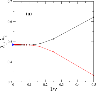
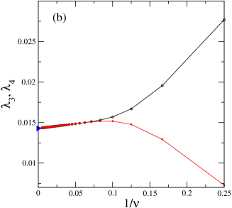
Figure 1: a) First (black line) and second (red line) eigenvalues of $\rho_{2}^{(1)}$ for $N=2$ as a function of $1/\nu$. b) Third (black line) and fourth (red line) eigenvalues of $\rho_{2}^{(1)}$ for $N=2$ as a function of $1/\nu$. The asymptotic degenerated values are shown by a blue triangle

Note that the $(2n+1)\times(2n+1)$ 1-RDM is a real symmetric matrix with two blocks, one $(n+1)\times(n+1)$ even block and one $n\times n$ odd block. For the case $n=1\Rightarrow\nu=2$ the matrices are $2\times 2$ and $1\times 1$ respectively, and its entries can be calculated analytically using equations (17-III). The normalization constant is $C_{2,2}\,=\,\frac{1}{\sqrt{3\pi}}\,$, the non-zero coefficients for the Hermite expansion equation (17) are

$$A^{(0)}_{0,0}\,=\,\pi^{1/4}\;;\;A^{(0)}_{1,1}\,=\,2\pi^{1/4}\;;\;A^{(1)}_{1,0}\,=\,A^{(1)}_{0,1}\,=\,\sqrt{2}\pi^{1/4}\;;\;A^{(2)}_{1,1}\,=\,\sqrt{8}\pi^{1/4}\,,$$ (29)

all the others are zero. Then, from equation (21), the non-zero coefficients of the wave-function expansion equation(20) are

$$a_{0,0}\,=\,\frac{1}{\sqrt{3}},\;a_{0,2}\,=\,a_{2,0}\,=\,\frac{1}{\sqrt{6}},\;a_{1,1}\,=\,\frac{1}{\sqrt{3}}\,.$$ (30)

The complete matrix is

$$\left[\rho_{2}^{(1)}\right]\,=\,\left(\begin{array}[]{ccc}\frac{1}{2}&0&\frac{1}{3\sqrt{2}}\\ 0&\frac{1}{3}&0\\ \frac{1}{3\sqrt{2}}&0&\frac{1}{6}\end{array}\right)\,,$$ (31)

whose eigenvalues are

$$\lambda_{\pm}\,=\,\frac{2\pm\sqrt{3}}{6}\;;\;\lambda_{2}\,=\,\frac{1}{3}\,.$$ (32)

Of course, for $n>1$, even though the $1$-RDM was obtained analytically, the eigenvalues must be calculated numerically.

In figure 1a) the two largest eigenvalues of $\rho$ are shown against $1/\nu$, and in figure 1b) the third and fourth eigenvalues.

In the strong interaction limit $\nu\to\infty$ the eigenvalues become doubly degenerate and can be calculated within the harmonic approximation HA2015 (which becomes exact in this limit) to be given by asymptotic formulas

$$\lambda_{2k+1,2k+2}^{\nu\rightarrow\infty}=2\sqrt{2}(3-2\sqrt{2})(17-12\sqrt{2})^{k},~{}~{}~{}~{}k=0,1,\ldots.$$ (33)

For the lowest occupancies we obtain $\lambda_{1}^{\nu\rightarrow\infty}=\lambda_{2}^{\nu\rightarrow\infty}=2\sqrt{2}(3-2\sqrt{2})\approx 0.485281$, $\lambda_{3}^{\nu\rightarrow\infty}=\lambda_{4}^{\nu\rightarrow\infty}=2\sqrt{2}(99-70)\sqrt{2})\approx 0.0142853$. The eigenvalues $\lambda_{1},\;\lambda_{2}$ coincide to 15 digits ((real(8) precision) for $n\geq 22$, and $\lambda_{3},\;\lambda_{4}$ for $n\geq 25$ with the asymptotic values.

The von Neumann entropy is shown in figure 2 a), and the linear entropy in figure 2b) for $n=1,\ldots,50$. We note that the entropies have a maximum between $n=2$ and $n=3$. Using the analytical formula for $\lambda_{k}^{\nu\rightarrow\infty}$ (33) and performing the summation in the formulas (25), the asymptotic values of the entropies can be calculated. The asymptotic value of the linear entropy is determined as

$$L_{2}^{{}^{\nu\rightarrow\infty}}=1-2\sum_{k=1}^{\infty}[\lambda_{k}^{\nu\rightarrow\infty}]^{2}=1-{\sqrt{2}\over 3}\approx 0.528595,$$ (34)

and the asymptotic value of the von Neumann entropy as being equal to

$$S_{2}^{\nu\rightarrow\infty}=-2\sum_{k=1}^{\infty}\lambda_{k}^{{}^{\nu\rightarrow\infty}}\mbox{log}_{2}\lambda_{k}^{{}^{\nu\rightarrow\infty}}=\frac{3\log_{2}\left(3+2\sqrt{2}\right)}{2\sqrt{2}}-\frac{3}{2}\approx 1.19737.$$ (35)

The exact values plotted in figure 2 approach nicely those limits.

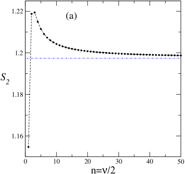
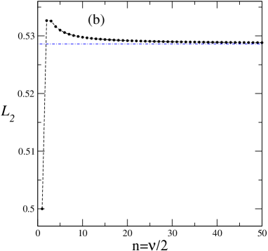
Figure 2: a) von Neumann entropy for $N=2$. b) Linear entropy for $N=2$. The asymptotic values are indicated by the dash-dotted blue lines.

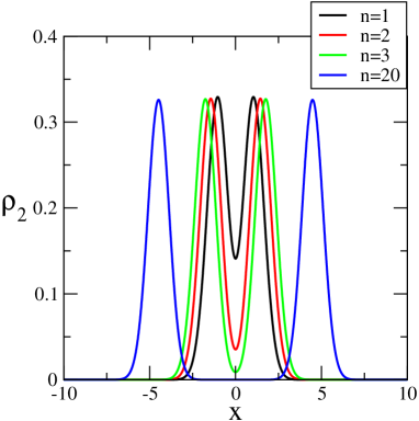
Figure 3: One-particle density $\rho_{2}(x)$ for $N=2$ and $n=1,2,3,20$.

Finally, in figure 3 we show the one-particle density for $n=1,2,3,20$. The one-particle density is an even function of the position, as can be expected from the symmetries of the Hamiltonian. The two-peaked one-particle density explains, at some extent, the behavior of the largest eigenvalues of the entanglement spectrum, as shown in figure 1, since for large enough values of $n$ it is easy to envisage that the eigenfunctions of the reduced density matrix that corresponds to the two largest eigenvalues should be, approximately, two peaked functions whose peaks should coincide with the peaks of the RDM, one of the then even and the other one odd and that for large enough $n$ both functions should weight more or less the same when the spectral decomposition of the RDM is considered. This reasoning applies when the two peaks of the one-particle density are well separated by a region where its magnitude is negligible. Of course, this is not the case for small values of $\nu$, where the height of the two peaks is not so different from the value of the particle density at the origin. Note that, because the wave function vanishes for $x_{1}=x_{2}$, the one-particle density has two peaks even in the limit $\nu\rightarrow 1$.

V The three, four and five-boson Calogero model

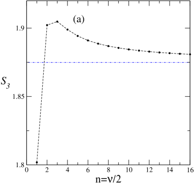
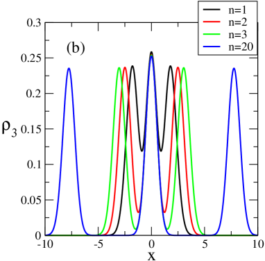
Figure 4: a) von Neumann entropy for $N=3$, the asymptotic value is indicated by the dash-dotted blue line. b) One-particle density $\rho_{3}(x)$ for $N=3$ and $n=1,2,3,20$

For $N>2$, even though the $p$-RDM was obtained analytically, the eigenvalues must be calculated numerically. Despite its elegant and concise form, the evaluation of all the terms involved in equation 23 for increasing values of $N$ becomes very demanding, so we present results for $N$ up to five.

Figure 4a) shows the von Neumann entropy for N=3 and its asymptotic value $S_{3}^{\nu\rightarrow\infty}\approx 1.87494$ HA2015 ; HApc , and figure 4b) the one-particle density for $n=1,2,3,20$.

As can be easily appreciated from figure 4a), the behavior of the von Neumann entropy is quite similar to the behavior already found for the case with $N=2$. Once again the most easily recognizable feature is the maximum that is attained near $n=3$. Figure 4b) shows the particle density as a function of $n$. As can be expected, the particle density has three well defined peaks, one of them centered in the origin of the coordinate axis and the other two placed symmetrically to both sides of the origin. The particle density is broader, as a function of the coordinate, for three particles than for only two, reflecting the fact that the repulsive term is stronger because the extra particle.

The von Neumann entropy of the 1-RDM is a increasing function of the particle number as can be appreciated in figure 5a). All the curves shown in figure 5a) have a maximum, and $S_{N}<S_{N+1}<S_{N+2}<\ldots$ irrespective of the values of the interaction parameter $\nu$. The maximum of the von Neumann entropy seems to appear for $\nu/2\in\left[2,4\right]$ irrespective of the number of particles considered, but since we are showing only those values that can be obtained analytically, it is quite possible that if $\nu$ can be varied continuously that the actual maximum is reached for a non-integer value of $\nu$ that depends on the number of particles.

From the data shown in figure 5a), it can be appreciated that the difference between successive values of the von Neumann entropy for a given value of $\nu$ decreases when $N$ is increased. Anyway, if the data is converging to some limit the increasing difficulty to evaluate the elements of 1-RDM and its eigenvalues prevented us from further exploring of this possibility.

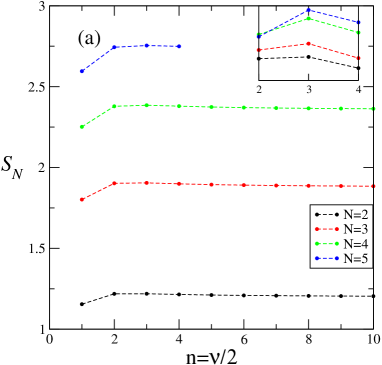
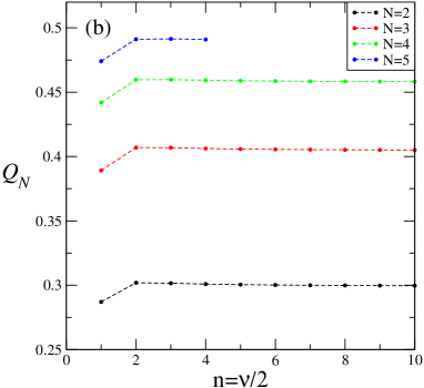
Figure 5: a) von Neumann entropy $S_{N}$, and b) JRW sub-entropy $Q_{N}$ for $N=2,3,4,5$. Inset: The von Neumann entropy always shows a maximum for $\nu/2\in\left[2,4\right]$, to visualize it we plot a detailed view of the different data sets. The peaks can be shown together by subtracting a constant quantity to each data set.

As has been said in the Introduction, there is a number of entropy-like functions that give information about the information content of the quantum states under study. We choose to explore the Jozsa-Robb-Wootters (JRW) sub-entropy Jozsa1994 , which is defined by

$$Q_{N}\,=\,-\sum_{k=1}^{(2n(N-1)+1)^{p}}\,\left(\prod_{j\neq k}\frac{\lambda_{k}}{\lambda_{k}-\lambda_{j}}\right)\lambda_{k}\,\log_{2}(\lambda_{k})\;.$$ (36)

since it gives a rigorous lower bound for the accessible information contained in the quantum state. This sub-entropy has been exactly calculated recently for a variant of the two-particle Moshinsky Hamiltonian gn13 .

In figure 5 b) we show $Q_{N}$ for the Calogero model for $N=2,3,4,5$. Note that $Q_{N}$ qualitatively similar to $S_{N}$, but $Q_{N}<<S_{N}$ in all the calculated values.

Interestingly, the JRW sub-entropy also shows the non-monotonous behavior shown by the von Neumann entropy and is too an increasing function of the particle number.

VI The two-fermion Calogero model

For two fermions we have an anti-symmetrical wave function

$$\Psi_{0}^{(F)}(x_{1},x_{2})\,=\,C_{\nu}\,sign(x_{1}-x_{2})\,\left|x_{1}-x_{2}\right|^{\nu}\,e^{-(x_{1}^{2}+x_{2}^{2})/2}\,,$$ (37)

where $C_{\nu}$ is a normalization constant. We note that, in this case we can ignore the absolute value when $\nu$ is a odd integer, and it is possible to calculate the normalization constant, then, for $\nu=2n+1$ we have

$$\Psi_{n}^{(F)}(x_{1},x_{2})\,=\,2^{n}\sqrt{\frac{2(2n+1)!}{\pi(4n+2)!}}\,\left(x_{1}-x_{2}\right)^{2n+1}\,e^{-(x_{1}^{2}+x_{2}^{2})/2}\,,$$ (38)

Even when the wave function is antisymmetrical, the 1-RDM is a symmetric operator, then its matrix elements could be written in a Hermite basis following the steps of the bosonic case.

In this case the the 1-RDM matrix is $(2n+2)\times(2n+2)$, decomposable in an even and an odd $(n+1)\times(n+1)$ blocks. For the case $n=1\Rightarrow\nu=3$ the matrices are $2\times 2$ and its eigenvalues can be calculated analytically. The complete matrix is

$$\left[\rho^{(1)}_{2}\right]\,=\,\left(\begin{array}[]{cccc}\frac{7}{20}&0&\frac{3}{10\sqrt{2}}&0\\ 0&\frac{9}{20}&0&\frac{1}{10}\sqrt{\frac{3}{2}}\\ \frac{3}{10\sqrt{2}}&0&\frac{3}{20}&0\\ 0&\frac{1}{10}\sqrt{\frac{3}{2}}&0&\frac{1}{20}\end{array}\right)\,,$$ (39)

whose eigenvalues are

$$\lambda_{\pm}\,=\,\frac{5\pm\sqrt{22}}{20}\,,$$ (40)

both with multiplicity 2. This is a general property that holds for all $n$ because both, the even and odd $(n+1)\times(n+1)$ blocks of the 1-RDM are different but isospectral matrices.

The von Neumann entropy for two fermions is shown in figure 6, the bosonic entropy was also included for comparison. Note that, at first and despite their closeness, both sets of points belong to different curves (the 1-RDMs are different) yet, because the strong repulsion between particles, the boson and fermion properties are almost coincident for large values of the coupling strength $\nu$. The quantitative differences between eigenvalues are largest in the neighborhood of the non-interacting limit $\nu\rightarrow 1$. This behavior is opposite to the one observed in the Moshinsky model where the difference between bosons and fermions is most noticeable for strong coupling Schilling ; Benavides .

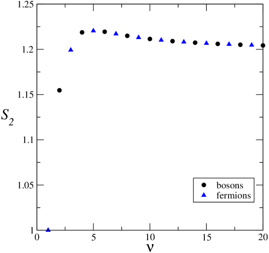
Figure 6: von Neumann entropy for $N=2$ for bosons ($\nu=2n$, solid black dots) and fermions ($\nu=2n+1$, solid blue triangles).

VII Discussion and Conclusions

As we have said previously, since the work of Moshinsky dealing with how much an approximate two-particle wave function actually resembles the exact solution of the problem, the need of benchmarks were an approximation scheme to obtain the information content of a problem can be tested has become more and more pressing. In CV problems the usual criteria used to qualify the accuracy of a given approximation are, basically, spectral, i.e if the approximate eigenvalues found using the approximation are accurate in some sense then it is assumed that the wave function and its information content should be accurate too. We think that the exact results presented in this work can contribute as a benchmark where to test some approximation schemes.

Katsura and Hatsuda, some years ago, have obtained an exact formal expression for the $p$-RDM of the $N$-particle Calogero-Sutherland model on a ring of finite perimeter Katsura2007 . They were able to write the $p$-RDM as a sum of products of functions where, in each term, the dependencies with both sets of variables of the $p$-RDM is factorized, as in equation (III). In that equation, the $p$-RDM depends on the sets of variables $\left\{x_{i}\right\}_{p}$ and $\left\{y_{j}\right\}_{p}$. Surprisingly, in the expression of Katsura and Hatsuda, each term contains the exact ground state of their model, $\psi_{0}^{CS}$, through products of the form $\overline{\psi_{0}^{CS}(\left\{x_{i}\right\}_{p})}\;\psi_{0}^{CS}(\left\{y_{j}\right\}_{p})$, instead of the completely factorized expression shown in equation III, where each term depends on a product of Hermite functions that depend in one, and only one, of the variables $x_{i}$ or $y_{j}$. This fact, owed to the Vandermonde determinant, allows us to find much more tractable expressions for the $p$-RDM than those found by Katsura and Hatsuda. If $N$ goes to infinity, both expressions, ours and the one of Katsura and Hatsuda, become formal since its evaluation becomes extremely troublesome. Although they provide an upper-bound for the entropy in this case, it is valid only in the thermodynamic limit.

Despite that the present works deals with the one-dimensional Calogero model, its extension to three dimensional problems with zero angular momentum is rather direct. As a matter of fact, using the results presented above we could obtain exactly some particular values of the von Neumann entropy for the three dimensional two-particle Crandall atom. This model was studied by Manzano et al. Manzano2010 , but in their work the von Neumann entropy was calculated using an approximate Monte Carlo integration scheme. From our data we observe that the work of Manzano et al. predicts higher but very accurate values for the von Neumann entropy in those cases where our result applies.

On the other hand, it is interesting to note that a non-monotonous behavior for the von Neumann entropy was obtained for two-electron models using perturbation theory when the interaction between the electrons is strongly localized and weak Majtey2012 .

The von Neumann entropy of the two-particle three dimensional case is a non-decreasing function of the interaction strength, in contradistinction with the one dimensional case. We think that this is so because the particle “impenetrability”, which is typical of one-dimensional problems, does not allow the particles to access some spatial regions, while higher-dimensional problems do not posses this property. So far, we do not have a proof confirming this hypothesis. Work around this lines is in progress.

- (1) G. Chiribella and G. Adesso, Phys. Rev. Lett 112, 010501 (2014).
- (2) S. L. Braunstein and P. van Loock, Rev. Mod. Phys. 77, 513 (2005).
- (3) Quantum Information with Continuous Variables of Atoms and Light, edited by N. Cerf, G. Leuchs, and E. S. Polzik (Imperial College Press, London, 2007).
- (4) M. C. Tichy, F. Mintert and A. Buchleitner, J. Phys. B: At. Mol. Opt. Phys. 44, 192001 (2011).
- (5) M. Moshinsky, Am. J. Phys. 36, 52 (1968).
- (6) F. Calogero, J. Math. Phys. 10, 2191 (1969).
- (7) C. Amovilli and N. H. March, Phys. Rev. A 69, 054302 (2004).
- (8) W.K. Wootters, Phys. Rev. Lett. 80, 2245 (1998).
- (9) L. Amico, R. Fazio, A. Osterloh, and V. Vedral, Rev. Mod. Phys. 80, 517 (2008).
- (10) V. Vedral, Rev. Mod. Phys. 74, 197 (2002).
- (11) M.A. Nielsen and I. L. Chuang, Quantum Computation and Quantum Information (Cambridge University Press, Cambridge, 2000).
- (12) C.H. Bennett, G. Brassard, S. Popescu, B. Schumacher, J. A. Smolin and W. K. Wootters, Phys. Rev. Lett. 76, 722 (1996).
- (13) M. Horodecki, P. Horodecki and R. Horodecki, Phys. Rev. Lett. 80, 5238 (1998).
- (14) P. Horodecki and R. Horodecki, Quantum Information and Computation 1, 45 (2001).
- (15) G. Giedke, M. M. Wolf, O. Krüger, R. F. Werner, and J. I. Cirac, Phys. Rev. Lett. 91, 107901 (2003).
- (16) R. Jozsa, D. Robb and W.K. Wootters, Phys. Rev. A 49, 668 (1994).
- (17) S. R. Nichols and W. K. Wootters, Quantum Information and Computation 3, 1 (2003).
- (18) F. Iemini and R. O. Vianna, Phys. Rev. A 87, 022327 (2013)
- (19) N. Killoran, M. Cramer and M.B. Plenio, Phys. Rev. Lett. 112, 150501 (2014).
- (20) A.D. Gottlieb and N.J. Mauser, Phys. Rev. Lett. 95, 123003 (2005).
- (21) K. Byczuk, J. Kuneš, W. Hofstetter and D. Vollhardt, Phys. Rev. Lett. 108, 087004 (20012).
- (22) J. M. Zhang and M. Kollar, Phys. Rev. A 89, 012504 (2014).
- (23) O. Osenda and P. Serra, Phys. Rev. A 75, 042331 (2007).
- (24) A. Ferrón, O. Osenda, and P. Serra, Phys. Rev. A 79, 032509 (2009).
- (25) F. M. Pont, O. Osenda, J. H. Toloza, and P. Serra, Phys. Rev. A 81, 042518 (2010).
- (26) A. P. Majtey, A. R. Plastino and J. S. Dehesa, J. Phys. A: Math. Theor. 45, 115309 (2012).
- (27) H. Li and F. D. M. Haldane, Phys. Rev. Lett. 101, 010504 (2008).
- (28) P. Calabrese and A. Lefevre, Phys. Rev. A 78, 032329 (2008).
- (29) D. Manzano, A. R. Plastino, J. S. Dehesa and T. Koga, J. Phys. A: Math. Theor. 43, 275301 (2010).
- (30) S. Pruski, J. Maćkowiak, O.Missuno, Rep. Math. Phys. 3, 241 (1972).
- (31) P. Kościk and A. Okopińska, Few-body Syst. 54, 1637 (2013).
- (32) C. Schilling, Phys. Rev. A 88, 042105 (2013).
- (33) C. L. Benavides-Riveros, I. V. Toranzo and J. S. Dehesa, Phys. B: At. Mol. Opt. Phys. 47, 195503 (2014).
- (34) B. Sutherland, J. Math. Phys. 12, 246 (1971).
- (35) P. J. Forrester and S. O. Warnaar, Bull. Am. Math. Soc. 45, 489 (2008).
- (36) S. K. Lando and A. K. Zvonkin, Graphs on Surfaces and Their Applications , Springer (2004).
- (37) L Carlitz, Monatshefte für Mathematik 66,393 (1962).
- (38) see, for example, S.G. Mikhlin, Integral Equations, Pergamon Press (1957).
- (39) P. Kościk, Phys. Lett. A 379, 293 (2015).
- (40) P. Kościk, private comunication.
- (41) S.D. Bajpai, http://www.sbc.org.pl/Content/33926/1992_03.pdf.
- (42) M.L. Glasser and I. Nagy, Phys. Lett. A 377, 2317 (2013).
- (43) H.Katsura and Y. Hatsuda, J. Phys. A: Math. Theor. 40, 13931 (2007)