On-shell diagrammatics and the perturbative structure of planar gauge theories

arXiv:1510.xxxx

October 2015

1 Introduction

Our understanding of perturbation theory in particle physics is mainly based on its Lagrangian formulation and the related Feynman diagrammatics which allows to compute relevant observables such as correlation functions and scattering amplitudes. In general, choosing a certain formulation of a theory boils down to establish the basic foundational hypothesis our construction is based on.

The point of view we are most accustomed to is to have unitarity and locality as manifest as possible – and thus they are part of the fundamental set of assumptions – which typically associates redundancies to the description, such as the gauge ones and field redefinitions, while any physical quantity is invariant under gauge and field-redefinition choices.

This enhanced freedom in the description, despite of the undeniable success in the exploration of physical processes, turns out to obscure a great deal of structure of the theory itself. This was already suggested by both simple [1] and recursive formulas [2, 3, 4, 5, 6, 7] for scattering amplitudes of gluons, which are much simpler than what could have been hoped from the Feynman expansion.

In the last years, the situation became more and more surprising both for general theories and, in particular, for the planar sector of $\mathcal{N}\,=\,4$ supersymmetric Yang-Mills theory. In the former case the development of a very general method to explore the perturbative regime, such as the BCFW-like deformations [8, 9, 10, 11, 12, 13], revealed tree-level recursive structures for a quite large class of theories, while in the latter direct loop integral analysis have shown that the theory is endowed with a further symmetry, the dual conformal symmetry [14, 15] (which together with the space-time conformal symmetry forms the infinite dimensional Yangian [16]), as well as the theory turns out to an on-shell recursion relation at integrand level [17] at all loops.

The existence of such a type of recursion relation implies that the amplitudes are determined in terms of the smallest non-trivial object at all order in perturbation theory and for any number of external states. Such a building block is provided by the three-particle amplitudes which are fixed, up to a coupling constant, by (super)-Poincaré invariance [18, 19]. Therefore one can turn the table around and start with the three-particle amplitudes, which, as we just saw, are fixed from first principles, and reconstruct more complicated amplitudes just in terms of these building blocks via a prescription which suitably glues them together [20]. This shows that it is possible to define a physical observable without resorting to the idea of a Lagrangian, and the Feynman diagrammatics is replaced by on-shell processes, i.e. objects whose states are always and all on-shell. As a consequence the objects one deals with are always physical and gauge invariant (contrarily to what happens with the Feynman expansion where the individual diagrams break gauge invariance and thus they cannot be considered as physical in a generic point of momentum space) and there is no need to introduce the idea of virtual (off-shell) particles. A further feature is that locality is generally broken for an individual on-shell process and it is then restored once all these on-shell processes are summed up to provide a scattering amplitude. This is not really a drawback given that it is exactly the manifest locality and unitarity that forces to introduce all the redundancies which the Lagrangian description is plagued of. However, this is not the end of the story. The gluing procedure which allows to generate higher-point/more complex on-shell processes turns out to preserve Yangian invariance [20] so that it is no longer hidden. This is particularly evident if one describes our objects in momentum twistor space or as an integral over the Grassmannian $G(k,n)$ [21, 22]. However, the connection between the on-shell processes and the Grassmannian appears to be much deeper: on-shell diagrams are related to a particular stratification of the positive Grassmannian $G(k,n)$ whose positivity-preserving diffeomorphisms represent the Yangian invariance of the amplitudes [20]. Furthermore, the on-shell diagrams turns out to be intimately related to permutations, which define equivalence classes for such objects, and whose adjacent transpositions encode the BCFW deformation [20] .

This picture however makes both unitarity and locality somehow hidden rather than emergent. However it can be encoded in a more general framework where the fundamental object is a new geometrical quantity, the amplituhedron [24], which can be though of as a generalisation of the notion of polytopes in momentum twistor space. The amplitudes are then read off as volumes, and both locality and unitarity emerge from the positivity of the geometry [25, 26, 27, 28]. Again, the quantities which can be computed at the end of the day are always the integrands of the amplitudes themselves.

What we have been describing so far, as already mentioned, holds just for planar $\mathcal{N}\,=\,4$ SYM theory, while the exploration of the non-planar structure started more recently [29, 30, 31, 32].

Beyond planar $\mathcal{N}\,=\,4$ SYM very little is known, with the exception of the ABJM theory in three dimensions where an analogous Grassmannian formulation have been discussed [20, 33, 34, 35, 36].

A question that is fair to ask is whether a general first principle picture is available for a larger class of theories, which does not make any reference to a Lagrangian and makes as many structures manifest as possible.

Indeed on-shell diagrams can be defined in general, i.e. with no reference to a specific theory: the three-particle building blocks are fixed by Poincaré symmetry for general helicities [18] and the prescription for gluing them and generate higher-point/more complex diagrams is not really theory dependent given that it boils down to integrate out the degrees of freedom on the intermediate lines according to the momentum conservation and on-shell condition constraints. However, there are important issues with would need to be addressed.

First of all, there are some theories for which there is no BCFW deformation available which returns a recursion relations at least for some amplitudes already at tree level. Recursive structures can be found by either using more general deformations [13] or by introducing further data [37]. In any case, this suggests that, if also in those cases a(n almost) first principle on-shell description is possible, there is a modification needed which takes into account this issue. Secondly, the loop analysis is even more subtle. It is necessary to unambiguously define an object representing the integrand, which in $\mathcal{N}\,=\,4$ SYM was possible mainly because of colour ordering – colour ordering allows to unambiguously fix the loop degrees of freedom among the various possible terms. Indeed this still holds for planar theories, but it is not clear how to get rid of such an ambiguity for theories whose amplitudes have no ordering whatsoever. This is not however the only issues which needs to be solved in order to have a clear identification between on-shell diagrams and scattering amplitudes. The loop singularity structure is intimately tied to the single cuts, which is in general a very ill-defined procedure: even if they vanish in dimensional regularisation, one is forced to consider also loops in the external states, which we will refer to as external on-shell bubbles, which makes ill-defined the single cut by producing a singularity of type $1/(p^{2})^{2}$. In $\mathcal{N}\,=\,4$ SYM theory, as well as in massless $\mathcal{N}\,\geq\,1$ and massive $\mathcal{N}\,\geq\,2$, this issue does not arise because these terms vanish upon summation over the full super-multiplet [40]. Thus, for a general theory, this issue need to be faced. While on one side one might naively neglect this type of terms because a regularisation prescription for the integrals would take care of them, on the other side, the contributions with external on-shell bubble at a certain order could contribute as internal loop at higher order. Thus one should either show that somehow this does not occur, or provide a prescription for the treatment of these terms.

In this paper we begin the investigation of the on-shell diagrammatics and the related mathematical structures for theories less special then the maximally supersymmetric ones. In order to reduce the number of ambiguities, for the time being we focus just on planar $\mathcal{N}\,<\,4$ gauge theories: In this way we indeed have a well defined object, the integrand, which can be represented via on-shell processes, as well as also the forward limits are well-defined, except for the non-supersymmetric case, i.e. pure Yang-Mills theory.

We focus in particular on the on-shell diagrammatics itself and its relation to the scattering amplitudes – a full-fledge (algebraic) geometrical discussion will be discussed in a companion paper [41]. Differently from the maximally supersymmetric case where the asymptotic states are provided by just single multiplets, the asymptotic states of less supersymmetric cases are represented via two multiplets, which are labelled by the helicity (the multiplets groups states with the same helicity sign). Therefore, the on-shell diagrammatics needs to account of these extra data. We discuss in detail such a decorated diagrammatics, pointing out the existence of directed helicity flows with a well-defined physical meaning. Importantly, the existence of these helicity flows identifies both the presence of singularities and their class. Furthermore, through them it is possible to define equivalence classes for the decorated on-shell diagrams.

Once the decorated on-shell diagrammatics has been set up, we establish the link between the decorated on-shell processes and the scattering amplitudes for $\mathcal{N}\,\leq\,2$ supersymmetric gauge theories. We investigate the information about the perturbative structure of the theory that the on-shell processes can encode. In particular, we provide a fully on-shell proof that for $\mathcal{N}\,=\,1,\,2$ supersymmetric (massless) Yang-Mills theories, the all-loop structure of the scattering amplitudes is fixed by the knowledge of the factorisation and forward singularities. Even if this was expected, there are many subtleties that need to be faced. First of all, even for supersymmetric theories, the forward limit is not well-defined and it is necessary to introduce a suitable regularisation scheme. Secondly, a single BCFW bridge turns out to be able to capture the complete cut-constructible information but not all the potentially problematic terms. In other words, there is a(n in principle) finite contribution from the boundary term at infinity. As a part of the regularisation scheme, we provide a prescription to actually include such terms. With such a completion, we show that those terms which were in principle problematic, upon summation, are of order $\mathcal{O}(\epsilon)$ ($\epsilon$ being the regularisation parameter) at all loops. For pure Yang-Mills, we discuss in detail the one-loop structure, for which, upon regularisation of the forward limit, it is possible to identify the on-shell bubbles as related to poles in the regularisation parameter. In order to obtain the full integrand, one has also to introduce a mass-deformation of the forward states.

The paper is organised as follows in Section 2 we provide a detailed description of the decorated on-shell diagrammatics and the meaning of the helicity flows, putting them in correspondence with certain singularities. In Section 3 we discuss the connection between the decorated on-shell diagrams and combinatorics. In particular, as in the maximally supersymmetric case, there exist equivalence relations between diagrams. In this section we discuss how also in this case permutations define equivalence classes of on-shell processes, with the crucial difference that they are selected by the helicity flows. Section 4 is devoted to the connection between decorated on-shell processes and scattering amplitude. We discuss the singularity structure both at tree and loop level, as well as we introduce a regularisation scheme to make sense of the forward limit on general grounds. We provide the on-shell proof that, for (massless) $\mathcal{N}\,=\,1,\,2$ SYM the all loop structure can be determined from factorisation and forward singularities upon suitable regularisation, with the potentially problematic terms which upon summation become of order $\mathcal{O}(\epsilon)$. We also discuss the loop structure for pure Yang-Mills mainly focusing on the one loop. Finally Section 5 contains our conclusion and outlook.

2 Decorated on-shell diagrammatics

Let us consider scattering processes in asymptotically Minkowski space-times for planar gauge theories with $\mathcal{N}\,\leq\,2$ supersymmetries. In a regime where asymptotic states can be defined, the latter are provided by the irreducible representations of the Poincaré group and they are taken to be the direct product of eigenstates of the momentum operator. Among the unitary representations, we will only deal with the ones whose states are eigenfunctions of the rotation generator of the massless Lorentz little group $iso(2)$ – the helicity operator – and are annihilated by the translation generators of $iso(2)$.

Given the isomorphism between the universal covering of the Lorentz group and $SL(2\,,\mathbb{C})$, the kinematics can be encoded into the spinors $\lambda_{a}$ and $\tilde{\lambda}_{\dot{a}}$, with the first spinor transforming in the fundamental representation of $SL(2\,,\mathbb{C})$ and the second one in the anti-fundamental representation. In the complexified momentum space, the universal covering of the Lorentz group is isomorphic to $SL(2\,,\mathbb{C})\,\times\,SL(2\,,\mathbb{C})$ and the two spinors $\lambda_{a}$ and $\tilde{\lambda}_{\dot{a}}$ transform under a different copy of $SL(2\,,\mathbb{C})$ each.

Taking as a convention that all the external states are incoming, the general structure of a scattering amplitude can therefore be written as

$$\mathcal{M}_{n}\>=\>\delta^{\mbox{\tiny$(2\times 2)$}}\left(\sum_{i=1}^{n}\lambda^{\mbox{\tiny$(i)$}}\tilde{\lambda}^{\mbox{\tiny$(i)$}}\right)M_{n}\left(\{\lambda^{\mbox{\tiny$(i)$}}\,,\tilde{\lambda}^{\mbox{\tiny$(i)$}}\,;h_{i}\}\right),$$ (2.1)

where the $\delta$-function implements momentum conservation, and $M_{n}$ is an analytic function of the Lorentz invariant combination of the spinors $\langle\lambda,\,\lambda^{\prime}\rangle\,\equiv\,\epsilon^{ab}\lambda_{a}\lambda^{\prime}_{b}$ and $[\tilde{\lambda},\,\tilde{\lambda}^{\prime}]\,\equiv\,\epsilon^{\dot{a}\dot{b}}\tilde{\lambda}_{\dot{a}}\tilde{\lambda}^{\prime}_{\dot{b}}$ as well as of the helicities $\{h_{i}\}$ of the external states . Being the latter eigenfunctions of the helicity operator $\hat{\mathcal{H}}^{\mbox{\tiny$(i)$}}$, we take $\hat{\mathcal{H}}^{\mbox{\tiny$(i)$}}$ to act on an amplitude as it acts on one-particle states

$$\hat{\mathcal{H}}^{\mbox{\tiny$(i)$}}\mathcal{M}_{n}\>=\>-2h_{i}\,\mathcal{M}_{n}.$$ (2.2)

The action of the Lorentz little group can also be seen as a momentum invariant rescaling of the spinors

$$(\lambda^{\mbox{\tiny$(i)$}},\,\tilde{\lambda}^{\mbox{\tiny$(i)$}})\,\longrightarrow\,(t_{i}\lambda^{\mbox{\tiny$(i)$}},\,t_{i}^{-1}\tilde{\lambda}^{\mbox{\tiny$(i)$}})\>\Longrightarrow\>M_{n}\left(t_{i}\lambda^{\mbox{\tiny$(i)$}}\,,t_{i}^{-1}\tilde{\lambda}^{\mbox{\tiny$(i)$}}\,;h_{i}\right)\>=\>t_{i}^{-2h_{i}}M_{n}\left(\lambda^{\mbox{\tiny$(i)$}}\,,\tilde{\lambda}^{\mbox{\tiny$(i)$}}\,;h_{i}\right).$$ (2.3)

In the case one wants to restrict to supersymmetric theories, it is more convenient to actually use the full Super-Poincaré group to define the asymptotic states [19]. If $Q_{Ia}$ and $\tilde{Q}^{I\dot{a}}$ are the super-charges, coherent states are defined as

$$|\lambda,\,\tilde{\lambda};\,\eta\rangle\>=\>e^{Q_{aI}w^{a}\eta^{I}}|\lambda,\,\tilde{\lambda};\,-1\rangle,\qquad|\lambda,\,\tilde{\lambda};\,\tilde{\eta}\rangle\>=\>e^{\tilde{Q}^{\dot{a}I}\tilde{w}_{\dot{a}}\tilde{\eta}_{I}}|\lambda,\,\tilde{\lambda};\,+1\rangle,$$ (2.4)

with $a,\,\dot{a}\,=\,1,2$ being the usual spinor indices, $I\,=\,1,\ldots,\,\mathcal{N}$ the R-symmetry index, while $w_{a}$ and $\tilde{w}_{a}$ are two spinors satisfying the conditions $\langle w,\,\lambda\rangle\,=\,1\,=\,[\tilde{w},\,\tilde{\lambda}]$, and $\eta^{I},\,\tilde{\eta}_{I}$ are Grassmann variables. Such coherent states are eigenstates of the super-charges:

$$Q_{aI}|\lambda,\,\tilde{\lambda};\,\tilde{\eta}\rangle\>=\>\lambda_{a}\tilde{\eta}_{I}|\lambda,\,\tilde{\lambda};\,\tilde{\eta}\rangle,\qquad\tilde{Q}_{\dot{a}I}|\lambda,\,\tilde{\lambda};\,\eta\rangle\>=\>\tilde{\lambda}_{\dot{a}}\eta_{I}|\lambda,\,\tilde{\lambda};\,\eta\rangle.$$ (2.5)

Except for the maximally supersymmetric case where the helicity states get organised into a single multiplet [19], for less supersymmetric theories there are two multiplets, which group the states with the same helicity sign and thus such a sign can be used to label them. Explicitly, for $\mathcal{N}\,\leq\,2$ they can be written as

$$\begin{split}&|\lambda,\,\tilde{\lambda};\,\eta,\,-\rangle\>=\>\sum_{s=0}^{\mathcal{N}}\frac{1}{s!}\left(\prod_{r=0}^{s}\eta_{\mbox{\tiny$I_{r}$}}\right)|\lambda,\,\tilde{\lambda};\,-(1-s/2)\rangle^{I_{1}\ldots I_{s}},\\ &|\lambda,\,\tilde{\lambda};\,\tilde{\eta},\,+\rangle\>=\>\sum_{s=0}^{\mathcal{N}}\frac{1}{s!}\left(\prod_{r=0}^{s}\tilde{\eta}^{\mbox{\tiny$I_{r}$}}\right)|\lambda,\,\tilde{\lambda};\,+(1-s/2)\rangle_{I_{1}\ldots I_{s}}.\end{split}$$ (2.6)

In the expression above we chose the $\eta$-representation for the negative multiplet and the $\tilde{\eta}$-representation for the positive one in such a way that the spin-$1$ state appeared as zero-order term in $\eta/\tilde{\eta}$. It is possible however to express both the multiplets in the same representation: the $\eta$- and $\tilde{\eta}$-representations are equivalent and they are related to each other by a Grassmann Fourier transform

$$\begin{split}&|\lambda,\tilde{\lambda};\,\eta,\,+\rangle\>=\>\int d^{\mathcal{N}}\tilde{\eta}\,e^{\tilde{\eta}\eta}|\lambda,\tilde{\lambda};\,\tilde{\eta},\,+\rangle\>=\>\sum_{s=0}^{\mathcal{N}}\frac{1}{s!}\left(\prod_{r=0}^{s}\eta_{\mbox{\tiny$I_{r}$}}\right)|\lambda,\tilde{\lambda};+\left(1-\frac{\mathcal{N}-s}{2}\right)\rangle^{I_{1}\ldots I_{s}},\\ &|\lambda,\tilde{\lambda};\,\tilde{\eta},\,-\rangle\>=\>\int d^{\mathcal{N}}\eta\,e^{\eta\tilde{\eta}}|\lambda,\tilde{\lambda};\,\eta,\,-\rangle\>=\>\sum_{s=0}^{\mathcal{N}}\frac{1}{s!}\left(\prod_{r=0}^{s}\tilde{\eta}^{\mbox{\tiny$I_{r}$}}\right)|\lambda,\tilde{\lambda};\,-\left(1-\frac{\mathcal{N}-s}{2}\right)\rangle_{I_{1}\ldots I_{s}}.\end{split}$$ (2.7)

With these coherent states at hand, we can consider them as asymptotic states for our scattering processes, and thus an amplitude can depend on $\eta$ and $\tilde{\eta}$. For each state, either of the two representations can be chosen. Furthermore, under little group transformations $\eta$ and $\tilde{\eta}$ behave as $\lambda$ and $\tilde{\lambda}$ respectively. In what follows, we choose the $\tilde{\eta}$-representation for all the states. Making supersymmetry invariance manifest, the structure of the amplitude (2.1) generalises to

$$\mathcal{M}_{n}\>=\>\delta^{\mbox{\tiny$(2\times 2)$}}\left(\sum_{i=1}^{n}\lambda^{\mbox{\tiny$(i)$}}\tilde{\lambda}^{\mbox{\tiny$(i)$}}\right)\delta^{\mbox{\tiny$(2\times\mathcal{N})$}}\left(\sum_{i=1}^{n}\lambda^{\mbox{\tiny$(i)$}}\tilde{\eta}^{\mbox{\tiny$(i)$}}\right)M_{n}(\{\lambda^{\mbox{\tiny$(i)$}},\,\tilde{\lambda}^{\mbox{\tiny$(i)$}};\,\tilde{\eta}^{\mbox{\tiny$(i)$}}\}),$$ (2.8)

with $M_{n}$ which just transforms under the action of the supersymmetric charge $\tilde{Q}$ via a shift of $\tilde{\eta}$.

2.1 Three-particle amplitudes

In the previous section, we have been discussing the construction of the asymptotic states from the representations of the (Super)-Poincaré group as well as some general properties of the amplitudes. As already mentioned, we will consider all states to be in the $\tilde{\eta}$-representation. The simplest objects that we can determine just by symmetries are the three-particle amplitudes: as the Poincaré invariance fixes them up to an overall constant [18], the Super-Poincaré group fixes the scattering of three coherent states [19]. In particular, momentum conservation can be written as

$$\langle i,j\rangle[i,j]\>=\>0,\qquad\forall\;i,\,j\>=\>1,\,2,\,3,$$ (2.9)

implying that either all the $\lambda$’s or the $\tilde{\lambda}$ are proportional to each other. Therefore, a given three-particle amplitude can either depend just on Lorentz invariant combinations of $\lambda$’s or of $\tilde{\lambda}$’s. Requiring that the amplitudes transform correctly under the Lorentz little group and supersymmetry as well as that they vanish on the real sheet, the explicit form of the three-particle amplitudes turns out to be

$$\begin{split}&\mathcal{M}_{3}^{\mbox{\tiny$(\mathfrak{1})$}}(1^{+},2^{+},3^{-})\>=\>\delta^{(2\times 2)}\left(\sum_{i=1}^{3}\lambda^{\mbox{\tiny$(i)$}}\tilde{\lambda}^{\mbox{\tiny$(i)$}}\right)\delta^{(1\times\mathcal{N})}\left(\sum_{i=1}^{3}[i+1,i-1]\tilde{\eta}^{\mbox{\tiny$(i)$}}\right)\frac{[1,2]^{4-\mathcal{N}}}{[1,2][2,3][3,1]},\\ &\mathcal{M}_{3}^{\mbox{\tiny$(\mathfrak{2})$}}(1^{-},2^{-},3^{+})\>=\>\delta^{(2\times 2)}\left(\sum_{i=1}^{3}\lambda^{\mbox{\tiny$(i)$}}\tilde{\lambda}^{\mbox{\tiny$(i)$}}\right)\delta^{(2\times\mathcal{N})}\left(\sum_{i=1}^{3}\lambda^{\mbox{\tiny$(i)$}}\tilde{\eta}^{\mbox{\tiny$(i)$}}\right)\frac{\langle 1,2\rangle^{4-\mathcal{N}}}{\langle 1,2\rangle\langle 2,3\rangle\langle 3,1\rangle},\end{split}$$ (2.10)

where the apex $(k)$ on the left-hand-side indicates the number of negative helicity multiplets, while $\mathcal{N}$ indicates the number of supersymmetries – notice that the expressions above reproduce the three-particle amplitudes for any $\mathcal{N}\,\leq\,4$. As already mentioned at the very beginning, we will just discuss the planar sector of the $\mathcal{N}\,\leq\,2$ supersymmetric theories, and thus all the amplitudes are understood to be colour ordered.

The three-particle amplitudes (2.10) can be actually thought as on-shell forms [20] by associating to them the super phase-space of each particle

$$\mathcal{A}_{3}^{\mbox{\tiny$(\mathfrak{k})$}}\>=\>\mathcal{M}_{3}^{\mbox{\tiny$(\mathfrak{k})$}}\prod_{i=1}^{3}\frac{d^{2}\lambda^{\mbox{\tiny$(i)$}}\,d^{2}\tilde{\lambda}^{\mbox{\tiny$(i)$}}}{\mbox{vol}\{GL(1)\}}d^{\mathcal{N}}\tilde{\eta}^{\mbox{\tiny$(i)$}}.$$ (2.11)

This turns out to be useful for gluing the three-particle amplitudes together, generating higher point on-shell processes.

At diagrammatic level, $\mathcal{M}_{3}^{\mbox{\tiny$(\mathfrak{1})$}}$ ($\mathcal{A}_{3}^{\mbox{\tiny$(\mathfrak{1})$}}$) and $\mathcal{M}_{3}^{\mbox{\tiny$(\mathfrak{2})$}}$ ($\mathcal{A}_{3}^{\mbox{\tiny$(\mathfrak{2})$}}$) are typically depicted as a white and a black trivalent nodes respectively, with the three lines departing from their centres representing the scattering states. Furthermore, we need to graphically distinguish between the negative- and positive-helicity multiplets. To this purpose, we conventionally decorate the three-particle diagrams by associating an incoming/outgoing arrow to the external lines to represent a negative/positive-helicity multiplet, as in Figure 1. Such a decoration provides the diagrams with a perfect orientation [42] to which it is possible to associate external nodes which the oriented arrows depart from (blue node, named source) or arrive to (red node, named sink).

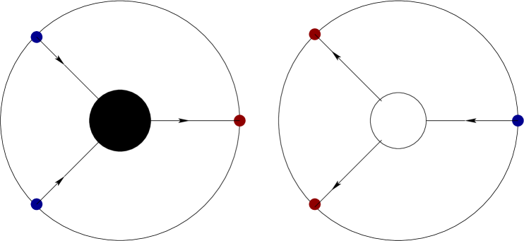
Figure 1: Decorated on-shell diagrams for three-particle amplitudes: The black and white nodes represent the MHV and $\bar{\mbox{MHV}}$ amplitudes respectively, while the incoming (outgoing) arrows represent the negative (positive) helicity multiplets. The decoration provides a perfect orientation which sources and sinks are associated to and identified by small dark blue and dark red nodes respectively at the boundary of the graph.

As a final comment, in the non-supersymmetric case a further set of tree-level amplitudes is allowed by Poincaré invariance (while supersymmetry forbids it)

$$\begin{split}\mathcal{M}_{3}^{\mbox{\tiny$(\mathfrak{0})$}}(1^{+},2^{+},3^{+})\>=\>\delta^{(2\times 2)}\left(\sum_{i=1}^{3}\lambda^{\mbox{\tiny$(i)$}}\tilde{\lambda}^{\mbox{\tiny$(i)$}}\right)\frac{[1,2][2,3][3,1]}{M^{2}},\\ \mathcal{M}_{3}^{\mbox{\tiny$(\mathfrak{3})$}}(1^{-},2^{-},3^{-})\>=\>\delta^{(2\times 2)}\left(\sum_{i=1}^{3}\lambda^{\mbox{\tiny$(i)$}}\tilde{\lambda}^{\mbox{\tiny$(i)$}}\right)\frac{\langle 1,2\rangle\langle 2,3\rangle\langle 3,1\rangle}{M^{2}},\end{split}$$ (2.12)

where the scale $M^{2}$ has been introduce to make explicit the dimensionfulness of the coupling constant of these amplitudes, i.e. the dimensionful coupling constant for such an operator has been replaced by a dimensionful one and the scale $M^{2}$. Their coupling constant is typically zero in pure Yang-Mills theory. However, the amplitudes (2.12) can appear in effective field theory – they correspond to a dimension six operator $\mbox{tr}\{F^{3}\}$ – or also in loop amplitudes where $M^{2}$ is actually given by a propagator [43]. In this last case, it is important to notice that they become highly singular: taken by themselves, because of the propagator-like factor, they diverge in the complexified momentum space, while they still vanish on the real-sheet, so they can in principle provide a finite quantity just when they get suitably glued to an object which would be vanishing in the complexified momentum space. Finally, taken $M^{2}$ not to have any kinematic dependence but just as a full-fledge dimensionful coupling constant, an eventual theory built up just from the amplitudes (2.12) seem to require the introduction of higher and higher dimension operators leading to the breakdown of locality [44]. In the following, we will build the planar non-supersymmetric spin-$1$ theory just out of the amplitude (2.10) and some comment on the emergence of (2.12) will eventually be made at loop level.

2.2 Building higher point diagrams

The isometry group of our space-time defined for us the simplest scattering process. Now we can use them to build more complicated on-shell processes. The most natural operation which can be defined is the gluing of two three-particle amplitudes or, more generally, of any two on-shell diagrams at hand, along one leg each. The natural prescription is to integrate over the super phase-space of the glued legs imposing momentum conservation and summing over all the coherent states which are allowed to propagate [20]:

$$\mathcal{M}_{m_{1}+m_{2}}\>=\>\sum_{h\,=\,\mp}\int\frac{d^{2}\lambda^{\mbox{\tiny$(P)$}}\,d^{2}\tilde{\lambda}^{\mbox{\tiny$(P)$}}}{\mbox{vol}\{GL(1)\}}d^{\mathcal{N}}\tilde{\eta}^{\mbox{\tiny$(P)$}}\mathcal{M}_{m_{1}+1}(-P,\,-h;\,\tilde{\eta}^{\mbox{\tiny$(P)$}})\mathcal{M}_{m_{2}+1}(P,\,h;\,\tilde{\eta}^{\mbox{\tiny$(P)$}}),$$ (2.13)

where the $\mathcal{M}$’s represent generic on-shell processes (they are not necessarily full-fledge amplitudes) and momentum conservation has been already implemented. This procedure is completely natural if one thinks of the on-shell processes as on-shell forms, as in (2.11): gluing two on-shell forms return a higher degree on-shell form. At a diagrammatic level this gluing prescription generates diagrams with a perfect orientation.

As just mentioned, the simplest higher point on-shell process which can be built is the four-point one obtained by gluing two three-particle amplitudes. It is possible to glue two three-particle amplitudes of different or of the same type.

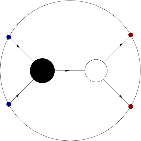
Figure 2: Simplest four-particle on-shell diagrams: Two on-shell $3$-forms are glued by integrating over the super phase-space of the internal on-shell leg. In this figure, this on-shell diagram appears having boundary nodes (and thus the four un-glued states are fixed): there is just a single coherent state which can propagate, and the integration over its super phase-space leads to a constraint on the external momenta.

In the first case (Figure 2), the integration over the super phase-space of the glued (intermediate) line returns a constraint on the momenta of the “un-glued states”, and it represents a singularity. Furthermore, if the external states are fixed, there is just one allowed coherent state propagating.

We can also glue together two three-particle amplitudes of the same type. In this case all the spinors of the same type in the whole (sub)-diagram turn out to be proportional to each other, which implies that it does not matter along which channel the four states are connected to each other. This defines an equivalence operation, dubbed merger [20], which allows to contract two three-particle amplitudes of the same type in a four-particle object along a channel and then expand it again along a different one. Notice that these equivalent four-particle (sub)-processes are characterised by three “external” states having a certain helicity while the fourth one to having the other, i.e. three arrows in the on-shell diagram has a certain direction, while the last one has the opposite decoration.

$$\raisebox{-25.6073pt}{\scalebox{0.4}{\includegraphics{4particleM.eps}}}\qquad\Longleftrightarrow\qquad\raisebox{-25.6073pt}{\scalebox{0.4}{\includegraphics{4particleM2.eps}}}\qquad\Longleftrightarrow\qquad\raisebox{-42.67912pt}{\scalebox{0.4}{\includegraphics{4particleM3.eps}}}$$

Figure 3: Merger operation: The proportionality among all the $\tilde{\lambda}$’s (all the $\lambda$’s in the case of two $\mathcal{M}_{3}^{\mbox{\tiny$(1)$}}$) implies that the four external states can be connected to each other equivalently in both channels. In each of such channels, just a single coherent state can propagate in the internal on-shell leg.

So far, there is no relevant difference with the maximally supersymmetric case: the gluing of two on-shell diagrams is defined according to the same prescription as well as the merger operation still holds. The first slight difference arises in this equivalence relation where just a certain multiplet can propagate as intermediate state.

2.3 BCFW bridges and helicity flows

Let us now discuss the general way to generate higher degree on-shell processes. Given a certain on-shell diagram $\mathcal{M}_{n}^{\mbox{\tiny$(0)$}}$ , it is always possible to single out two external lines and connecting them by gluing one three-particle amplitude to each of them, being of different type, and gluing those three-particle amplitudes between them. The integration over the delta-functions leaves one degree of freedom unfixed, mapping $\mathcal{M}_{n}^{\mbox{\tiny$(0)$}}$ to a (higher degree) differential form

$$\mathcal{M}_{n}^{\mbox{\tiny$(0)$}}\qquad\longrightarrow\qquad\mathcal{M}_{n}^{\mbox{\tiny$(1)$}}\>=\>dz\,\mu(z)\,\mathcal{M}_{n}^{\mbox{\tiny$(0)$}}(z),$$ (2.14)

where $\mathcal{M}_{n}^{\mbox{\tiny$(0)$}}(z)$ is nothing but the BCFW-deformed $\mathcal{M}_{n}^{\mbox{\tiny$(0)$}}$ (Figure 4) and $\mu(z)$ is a measure induced by the BCFW bridge itself.

$$\raisebox{-42.67912pt}{\scalebox{0.3}{\includegraphics{BCFWbridge1.eps}}}\hskip 28.45274pt\Longrightarrow\hskip 28.45274pt\raisebox{-42.67912pt}{\scalebox{0.3}{\includegraphics{BCFWbridge2.eps}}}$$

Figure 4: Generating higher degree diagrams via a BCFW bridge: From a given on-shell diagram (generically represented on the left-hand-side), a higher degree on-shell diagram can be generated attaching a BCFW bridge to two selected external states, i.e. they get connected via two three-particle amplitudes of different type which are glued to each other (on right-hand-side).

As prescribed, when this BCFW bridge is attached to a given on-shell diagram, one needs to sum over all the possible coherent states which can propagate. Typically, one is used to think of the BCFW deformations as preserving the helicities of the deformed states. Summing over all the allowed coherent states instead admits the possibility that this does not hold. Let us clarify this point. From a given on-shell diagram, let us single out two external states having different helicities and attach a BCFW bridge to them. There are two generally inequivalent ways to perform such an operation, which differ from each other dependently on which three-particle amplitude of the bridge is associated to each external coherent state.

Let us start with associating the anti-holomorphic (holomorphic) amplitude to the negative (positive) helicity external coherent state:

$$\raisebox{-48.36958pt}{\scalebox{0.33}{\includegraphics{BCFWbridgeA.eps}}}\>=\>\frac{dz}{z}\mathcal{M}_{n}^{\mbox{\tiny$(0)$}}(z),\hskip 56.9055pt\left\{\begin{array}[]{l}q_{\mbox{\tiny$ij$}}\>=\>z\lambda^{\mbox{\tiny$(i)$}}\tilde{\lambda}^{\mbox{\tiny$(j)$}},\\ \hat{p}^{\mbox{\tiny$(i)$}}\>=\>\lambda^{\mbox{\tiny$(i)$}}(\tilde{\lambda}^{\mbox{\tiny$(i)$}}-z\tilde{\lambda}^{\mbox{\tiny$(j)$}}),\\ \tilde{\eta}^{\mbox{\tiny$(\hat{i})$}}\>=\>\tilde{\eta}^{\mbox{\tiny$(i)$}}-z\tilde{\eta}^{\mbox{\tiny$(j)$}},\\ \hat{p}^{\mbox{\tiny$(j)$}}\>=\>(\lambda^{\mbox{\tiny$(j)$}}+z\lambda^{\mbox{\tiny$(i)$}})\tilde{\lambda}^{\mbox{\tiny$(j)$}}.\end{array}\right.,$$ (2.15)

where the upper vertical (intermediate) lines need to be thought of as attached to a putative on-shell diagram and have momenta $\hat{p}^{\mbox{\tiny$(i)$}}$ and $\hat{p}^{\mbox{\tiny$(j)$}}$, $q_{\mbox{\tiny$ij$}}$ is the momentum in the horizontal intermediate line connecting the two three-particle amplitudes, while the lower lines are external states with momenta $p^{\mbox{\tiny$(i)$}}$ and $p^{\mbox{\tiny$(j)$}}$. With such a choice, there is only one coherent state which can propagate in the each intermediate line. As it is straightforward to see from (2.15), this BCFW bridge induces a BCFW deformation on the on-shell diagrams which deforms the positive/negative helicity spinor of the negative/positive helicity multiplet of the given on-shell process. Furthermore, a well-defined helicity flow can be identified from the external coherent states to the on-shell diagram the BCFW bridge is applied to.

Let us now consider a BCFW bridge obtained from the previous one by exchanging the holomorphicity of the three-particle amplitudes in the bridge (the helicities of the external states are always kept fixed). In this case, two possible coherent states are admitted in the intermediate lines

$$\raisebox{-51.21504pt}{\scalebox{0.33}{\includegraphics{BCFWbridgeB.eps}}}\quad+\quad\raisebox{-51.21504pt}{\scalebox{0.33}{\includegraphics{BCFWbridgeC.eps}}},\hskip 56.9055pt\left\{\begin{array}[]{l}q_{\mbox{\tiny$ij$}}\>=\>z\lambda^{\mbox{\tiny$(j)$}}\tilde{\lambda}^{\mbox{\tiny$(i)$}},\\ \hat{p}^{\mbox{\tiny$(i)$}}\>=\>(\lambda^{\mbox{\tiny$(i)$}}-z\lambda^{\mbox{\tiny$(j)$}})\tilde{\lambda}^{\mbox{\tiny$(i)$}},\\ \hat{p}^{\mbox{\tiny$(j)$}}\>=\>\lambda^{\mbox{\tiny$(j)$}}(\tilde{\lambda}^{\mbox{\tiny$(j)$}}+z\tilde{\lambda}^{\mbox{\tiny$(i)$}})\\ \tilde{\eta}^{\mbox{\tiny$(\hat{j})$}}\>=\>\tilde{\eta}^{\mbox{\tiny$(j)$}}-z\tilde{\eta}^{\mbox{\tiny$(i)$}}.\end{array}\right.\;.$$ (2.16)

Let us consider these two contributions separately. As far as the first one is concerned, it provides the same differential as (2.15) (even if the on-shell diagram the bridge is attached to gets deformed in a different way) and there is a well-defined helicity flow from the external coherent states to the on-shell diagram the BCFW bridge is attached to, as in the previous case

$$\raisebox{-48.36958pt}{\scalebox{0.33}{\includegraphics{BCFWbridgeB.eps}}}\>=\>\frac{dz}{z}\mathcal{M}_{n}^{\mbox{\tiny$(0)$}}(z).$$ (2.17)

Thus, this contribution induces the “conjugate” BCFW deformation of (2.15) on the on-shell diagram the bridge is attached to. Another feature that can be identified is the existence of a helicity flow along the intermediate lines in the left-hand-side of (2.17).

In the second contribution in (2.16), there is no helicity flow from the external lines and which connect the bridge to a putative on-shell diagram, while there is along the intermediate lines as in (2.17) but in opposite direction. Furthermore, differently from (2.15) and (2.17), the differential has a different structure

$$\raisebox{-48.36958pt}{\scalebox{0.33}{\includegraphics{BCFWbridgeC.eps}}}\>=\>dz\,z^{3-\mathcal{N}}\mathcal{M}_{n}^{\mbox{\tiny$(0)$}}(z).$$ (2.18)

Contrarily to the other cases just discussed, this contribution is not directly related to a BCFW deformation of the original on-shell diagram because of the change in helicity of the lines the bridge is attached to, and the differential shows a multiple pole. This for $\mathcal{N}\,\leq\,2$. For $\mathcal{N}\,=\,3$ the differential measure $\mu$ is just equal to $1$, while for the maximally supersymmetric case $\mathcal{N}\,=\,4$, also this bridge has the same measure $1/z$ as the other two, making it equivalent to the previous one in eq (2.17). Notice also that the differential (2.18) is not helicity blind for $\mathcal{N}\,\neq\,4$ (the degree of freedom labelled by $z$ transforms not trivially under the little group of $p^{\mbox{\tiny$(i)$}}$ and $p^{\mbox{\tiny$(j)$}}$), which implies that the helicity configuration of the on-shell diagram the bridge is attached to is different of the helicity configuration of the full on-shell diagram.

So far we have been discussing BCFW bridges whose external coherent states had different helicities. In order to complete this analysis, let us consider BCFW bridges whose external states have the same helicity. In this case, no matter how the bridge is formed, there is just one possible coherent state propagating in each intermediate line:

$$\begin{split}&\raisebox{-48.36958pt}{\scalebox{0.33}{\includegraphics{BCFWbridgeD.eps}}}\>=\>\frac{dz}{z}\mathcal{M}_{n}^{\mbox{\tiny$(0)$}}(z),\hskip 56.9055pt\left\{\begin{array}[]{l}q_{\mbox{\tiny$ij$}}\>=\>z\lambda^{\mbox{\tiny$(i)$}}\tilde{\lambda}^{\mbox{\tiny$(j)$}}\\ \hat{p}^{\mbox{\tiny$(i)$}}\>=\>\lambda^{\mbox{\tiny$(i)$}}(\tilde{\lambda}^{\mbox{\tiny$(i)$}}-z\tilde{\lambda}^{\mbox{\tiny$(j)$}}),\\ \tilde{\eta}^{\mbox{\tiny$(\hat{i})$}}\>=\>\tilde{\eta}^{\mbox{\tiny$(i)$}}-z\tilde{\eta}^{\mbox{\tiny$(j)$}}\\ \hat{p}^{\mbox{\tiny$(j)$}}\>=\>(\lambda^{\mbox{\tiny$(j)$}}+z\lambda^{\mbox{\tiny$(i)$}})\tilde{\lambda}^{\mbox{\tiny$(j)$}}\end{array}\right.\\ &\raisebox{-48.36958pt}{\scalebox{0.33}{\includegraphics{BCFWbridgeE.eps}}}\>=\>\frac{dz}{z}\mathcal{M}_{n}^{\mbox{\tiny$(0)$}}(z),\hskip 56.9055pt\left\{\begin{array}[]{l}q_{\mbox{\tiny$ij$}}\>=\>z\lambda^{\mbox{\tiny$(j)$}}\tilde{\lambda}^{\mbox{\tiny$(i)$}}\\ \hat{p}^{\mbox{\tiny$(i)$}}\>=\>(\lambda^{\mbox{\tiny$(i)$}}-z\lambda^{\mbox{\tiny$(j)$}})\tilde{\lambda}^{\mbox{\tiny$(i)$}}\\ \hat{p}^{\mbox{\tiny$(j)$}}\>=\>\lambda^{\mbox{\tiny$(j)$}}(\tilde{\lambda}^{\mbox{\tiny$(j)$}}+z\tilde{\lambda}^{\mbox{\tiny$(i)$}})\\ \tilde{\eta}^{\mbox{\tiny$(\hat{j})$}}\>=\>\tilde{\eta}^{\mbox{\tiny$(j)$}}-z\tilde{\eta}^{\mbox{\tiny$(i)$}}\end{array}\right.,\end{split}$$ (2.19)

as well as there is just a helicity flow between the external lines and the intermediate ones which glue the bridge with a putative on-shell diagram, the differential measure is as in (2.15) and (2.17).

It is important to stress here that the existence or not of helicity flows plays a very important role in identifying the physical structure of a theory. For the moment we have learnt that the presence of a helicity flow between the external lines of a BCFW bridge and the intermediate ones attached to a putative on-shell diagram correspond to the differential measure of $1/z$, while in absence of such a flow, it develops a multiple pole; when different states can propagate in the intermediate lines, a helicity flow in them is generated. How deep is this observation? In order to understand it, let us discuss the helicity flows more generally

2.4 On-shell diagrams and helicity flows

Let us consider the simplest (non-singular) on-shell diagrams, such as in Figure 5, where the helicity configuration $(-,+,-,+)$ has been chosen for the external coherent states. Notice that the second and third diagrams actually come from the sum over the coherent states which can propagate in the glued intermediate lines once the holomorphicity of the three-particle amplitude has been chosen. For the choice in the first diagram instead, just one coherent state per intermediate line is allowed.

                   

Figure 5: Simplest four-particle on-shell diagrams viewable in terms of a BCFW bridge attached to an other (simpler) on-shell diagram.

They can be considered as a BCFW bridge attached to a diagram of the type in Figure 2. The latter, providing a delta-function on the momenta, fixes the degree of freedom introduced by the bridge. Thus, these on-shell diagrams are fully localised and return a rational function of the Lorentz invariants. Let us notice that each of these on-shell diagrams can be viewed as generated by a BCFW bridge in two different channels. In order to be as explicit as possible, we discuss separately the three on-shell diagrams. Beginning with the first on-shell diagram in Figure 5, as we just mentioned it can be seen as a BCFW bridge applied in two different channels

           

Notice that each of them can be viewed in two different ways because each sub-diagram in which they have been virtually separated by the dashed red line can be thought as implementing a BCFW bridge. Following the helicity arrows, it is straightforward to realise that there exists a helicity flow between the external states and the intermediate one, while there is no helicity flow in the intermediate lines: all the possible BCFW bridges are of the type (2.15). Furthermore, each single sub-diagram has the same helicity configuration $(-,+,-,+)$ as the full diagram and the full diagram shows helicity flows between all the adjacent states. This is just the statement that the whole on-shell diagram contains all and only the singularities (simple poles) related to the helicity configuration $(-,+,-,+)$ with the correct residues. More explicitly, the fact that the full diagram shows helicity flows between all the adjacent external states implies that the physical object it represents contains all and only the complex factorisation in both the $s$- and $t$-channels

$$\begin{array}[]{cccccc}{}\hfil&{}\hfil&\raisebox{-39.83368pt}{\scalebox{0.3}{\includegraphics{4ptSing2a.eps}}}&+&\raisebox{-39.83368pt}{\scalebox{0.3}{\includegraphics{4ptSing2b.eps}}}&+\\ {\raisebox{-45.52458pt}{\scalebox{0.3}{\includegraphics{4ptHelFlow1.eps}}}}&{}\hfil&\begin{array}[]{ccc}{\color[rgb]{1,0,0}2}&\longleftarrow&{\color[rgb]{0,0,1}3}\\ \uparrow&{}\hfil&{}\hfil\\ {\color[rgb]{0,0,1}1}&\longrightarrow&{\color[rgb]{1,0,0}4}\end{array}&{}\hfil&\begin{array}[]{ccc}{\color[rgb]{1,0,0}2}&\longleftarrow&{\color[rgb]{0,0,1}3}\\ {}\hfil&{}\hfil&\downarrow\\ {\color[rgb]{0,0,1}1}&\longrightarrow&{\color[rgb]{1,0,0}4}\end{array}&{}\hfil\\ {}\hfil&{\Longrightarrow}&{}\hfil&{}\hfil&{}\hfil&{}\hfil\\ {\vspace{-.5cm}\begin{array}[]{ccc}{\color[rgb]{1,0,0}2}&\longleftarrow&{\color[rgb]{0,0,1}3}\\ \uparrow&{}\hfil&\downarrow\\ {\color[rgb]{0,0,1}1}&\longrightarrow&{\color[rgb]{1,0,0}4}\end{array}}&{}\hfil&\raisebox{-28.45274pt}{\scalebox{0.3}{\includegraphics{4ptSing2c.eps}}}&+&\raisebox{-28.45274pt}{\scalebox{0.3}{\includegraphics{4ptSing2d.eps}}}&{}\hfil\\ {}\hfil&{}\hfil&\begin{array}[]{ccc}{\color[rgb]{1,0,0}2}&{}\hfil&{\color[rgb]{0,0,1}3}\\ \uparrow&{}\hfil&\downarrow\\ {\color[rgb]{0,0,1}1}&\longrightarrow&{\color[rgb]{1,0,0}4}\end{array}&{}\hfil&\begin{array}[]{ccc}{\color[rgb]{1,0,0}2}&\longleftarrow&{\color[rgb]{0,0,1}3}\\ \uparrow&{}\hfil&\downarrow\\ {\color[rgb]{0,0,1}1}&{}\hfil&{\color[rgb]{1,0,0}4}\end{array}&{}\hfil\end{array}$$

Let us repeat the same analysis for the second on-shell diagram of Figure 5:

           

In the diagram on the left, it is possible to notice a helicity flow between the external lines and the intermediate one in the two possible BCFW bridges, and furthermore there is also a helicity flow along just the intermediate lines. As a consequence, each of the two sub-diagrams in this channel has the same helicity structure of the full diagram.

In the picture on the right, the very same diagram is viewed in a different channel. Here one can instead identify a helicity flow along the intermediate lines as well as one involving the two external lines of a bridge and the intermediate one connecting them, while there is no flow from the external lines to the ones attached to the other diagram. As a consequence, both of the two sub-diagrams do not preserve the helicity structure of the full diagram. This means that in this channel the on-shell diagram under discussion does not contain the right residue to represent a full-fledge four-particle amplitude. This information is encoded in the (clockwise) orientation of the helicity flow in the intermediate lines in the full diagram.

A similar analysis holds for the last diagram in Figure 5, where the helicity flow of the intermediate lines is counter-clockwise:

           

Summarising, the two diagrams just analysed (which, we do not have to forget, need to me summed up) shows two helicity flows between adjacent coherent states as well as a oriented helicity flows in the intermediate lines. The former implies that the full on-shell diagram contains a pole in the channel where the external helicity flow appears, while the latter that diagram also has structures related to different helicity configurations, which boils down to having higher order poles:

$$\begin{split}&\raisebox{-45.52458pt}{\scalebox{0.32}{\includegraphics{4ptHelFlow2.eps}}}\;\Longrightarrow\;\raisebox{-39.83368pt}{\scalebox{0.32}{\includegraphics{4ptSing1a.eps}}}\;+\;\raisebox{-39.83368pt}{\scalebox{0.32}{\includegraphics{4ptSing1d.eps}}}\;+\;\raisebox{-19.91684pt}{\scalebox{0.32}{\includegraphics{4ptSing1b.eps}}}\;+\;\raisebox{-19.91684pt}{\scalebox{0.32}{\includegraphics{4ptSing1c.eps}}}\\ &\raisebox{-45.52458pt}{\scalebox{0.32}{\includegraphics{4ptHelFlow3.eps}}}\;\Longrightarrow\;\raisebox{-39.83368pt}{\scalebox{0.32}{\includegraphics{4ptSing4a.eps}}}\;+\;\raisebox{-39.83368pt}{\scalebox{0.32}{\includegraphics{4ptSing4b.eps}}}\;+\;\raisebox{-19.91684pt}{\scalebox{0.32}{\includegraphics{4ptSing4c.eps}}}\;+\;\raisebox{-19.91684pt}{\scalebox{0.32}{\includegraphics{4ptSing4d.eps}}}\end{split}$$

where the red helicity flows indicate the ones characterising a different helicity configuration. Individually, these diagrams cannot represent the full-fledge four-particle amplitude with helicity configuration $(-,+,-,+)$ given that each of them shows just one factorisation channel. Their sum instead could, provided that suitable cancellations occur. As we will see later, those cancellations occur just for $\mathcal{N}\,=\,3$ (in the maximally supersymmetric case, there is no distinction between them).

For the sake of completeness, we explicitly consider the fully localised four-particle on-shell diagram with the helicity configuration $(-,-,+,+)$. Actually, as we will see, this class of diagram exhibits a property which is absent in the one analysed so far. It is easy to see that the helicity configuration $(-,-,+,+)$ for the external states allows for two diagrams only, as shown in Figure 6

             

Figure 6: Four-particle on-shell diagrams with external helicity configuration $(-,-,+,+)$

Notice that in none of them there is a helicity flow within the intermediate lines only. As for the previous class of on-shell diagrams, also in this case each diagram can be viewed as two BCFW-like bridges applied to another on-shell diagram:

$$\begin{split}&\raisebox{-25.6073pt}{\scalebox{0.4}{\includegraphics{4ptBCFWs4.eps}}}\hskip 34.14322pt\raisebox{-25.6073pt}{\scalebox{0.4}{\includegraphics{4ptBCFWt4.eps}}}\\ \phantom{\ldots}\\ &\raisebox{-25.6073pt}{\scalebox{0.4}{\includegraphics{4ptBCFWs5.eps}}}\hskip 34.14322pt\raisebox{-25.6073pt}{\scalebox{0.4}{\includegraphics{4ptBCFWt5.eps}}}\end{split}$$

In the on-shell diagrams on the left (both at the top and at the bottom) both the sub-diagrams preserve the helicity configuration of the full diagram and they show a helicity flow between the external states and the intermediate lines which get glued to the other diagram. In the on-shell diagrams on the right instead just one of the two sub-diagrams preserves the helicity configuration of the full diagram and it is also the only one which shows a helicity flow between the external lines and the ones which get glued to the other diagram.

$$\begin{split}&\raisebox{-45.52458pt}{\scalebox{0.3}{\includegraphics{4ptHelFlow4.eps}}}\;\Longrightarrow\;\raisebox{-39.83368pt}{\scalebox{0.32}{\includegraphics{4ptSing3a.eps}}}\;+\;\raisebox{-39.83368pt}{\scalebox{0.32}{\includegraphics{4ptSing3d.eps}}}\;+\;\raisebox{-39.83368pt}{\scalebox{0.32}{\includegraphics{4ptSing3c.eps}}}\\ &\raisebox{-45.52458pt}{\scalebox{0.3}{\includegraphics{4ptHelFlow5.eps}}}\;\Longrightarrow\;\raisebox{-39.83368pt}{\scalebox{0.32}{\includegraphics{4ptSing3a.eps}}}\;+\;\raisebox{-39.83368pt}{\scalebox{0.32}{\includegraphics{4ptSing3d.eps}}}\;+\;\raisebox{-39.83368pt}{\scalebox{0.32}{\includegraphics{4ptSing3c.eps}}}\end{split}$$

Furthermore, the diagram at the top and the one at the bottom are one the mirror of the other, i.e. they are topologically equivalent: they contain the same complex factorisation channels, as it is made manifest from the explicit channels above and as it can be deduced from the helicity flows.

$$\begin{split}&\raisebox{-25.6073pt}{\scalebox{0.3}{\includegraphics{4ptHelFlow1.eps}}}\hskip 28.45274pt\raisebox{-25.6073pt}{\scalebox{0.3}{\includegraphics{4ptHelFlow2.eps}}}\hskip 28.45274pt\raisebox{-25.6073pt}{\scalebox{0.3}{\includegraphics{4ptHelFlow3.eps}}}\\ &\phantom{\ldots}\\ &\hskip 68.28644pt\raisebox{-25.6073pt}{\scalebox{0.3}{\includegraphics{4ptHelFlow4.eps}}}\hskip 28.45274pt\raisebox{-25.6073pt}{\scalebox{0.3}{\includegraphics{4ptHelFlow5.eps}}}\end{split}$$

Figure 7: Helicity flows. For each possible diagram with external helicity configuration $(-,+,-,+)$ (at the top) and $(-,-,+,+)$ (at the bottom) all the helicity flows are shown.

The lesson we learn from this analysis is that the structure of the helicity flows reveals the possible equivalence between two on-shell (four-particle) diagrams related by an exchange of holomorphicity of their three-particle building blocks. In particular, such an equivalence holds just for the helicity configuration $(-,-,+,+)$, for which the helicities of the internal states are fixed once for all and there is no helicity flow along the internal lines.

Thus, together with the merger operation (Figure 3), the decorated diagrammatics enjoys a further equivalence relation, which is the less/no-supersymmetric counterpart of the square move in $\mathcal{N}\,=\,4$ SYM [20] and involves the coherent states in a precise ordering, i.e. the equal-helicity coherent states have to be adjacent (Figure 8).

$$\raisebox{-39.83368pt}{\scalebox{0.35}{\includegraphics{4ptDiag4.eps}}}\qquad\Longleftrightarrow\qquad\raisebox{-39.83368pt}{\scalebox{0.35}{\includegraphics{4ptDiag5.eps}}}$$

Figure 8: Square move operation. For non-maximally supersymmetric theories, it is possible to define an equivalence relation between two four-particle fully-localised diagrams if and only if the external multiplets with the same helicity are adjacent.

The limited validity of this equivalence relation is a further crucial difference with the maximally supersymmetric case.

In order to close this section, we need to discuss one further operation: the bubble deletion. Generally, the manipulation of a given on-shell diagram via mergers and square moves can lead to a sub-diagram in which two three-particle amplitudes share two lines. In the maximally supersymmetric case, this bubble could be replaced by a single intermediate line (the bubble could be deleted) with the price of generating a $d\log{\zeta}$ term: there is a change of variables mapping the bubble into a factored-out $d\log{\zeta}$ form. In the less/no-supersymmetric case, we need to distinguish two cases, depending on whether or not there is an oriented helicity flow inside the bubble. In absence of an oriented helicity flow inside the bubble, the two intermediate states have the same helicity: there exists a change of variable mapping the bubble into a single intermediate line with the same helicity arrow as the states in the bubble with a $d\log{\zeta}$ factor:

$$\raisebox{-11.38092pt}{\scalebox{0.45}{\includegraphics{BubbleDel1.eps}}}\qquad=\qquad\raisebox{0.0pt}{\scalebox{0.45}{\includegraphics{BubbleDel1rhs.eps}}}\quad d\log{\zeta}$$ (2.20)

If there is instead an oriented helicity flow, this is no longer possible. More precisely, an eventual change of variable which would allow to map the bubble into a single intermediate line factoring out the related degree of freedom is given by a transcendental equation. At most we can write the following schematic relation

$$\begin{split}&\raisebox{-11.38092pt}{\scalebox{0.45}{\includegraphics{BubbleDel2.eps}}}+\raisebox{-11.38092pt}{\scalebox{0.45}{\includegraphics{BubbleDel3.eps}}}\quad=\\ &\hskip 85.35826pt=\quad\raisebox{0.0pt}{\scalebox{0.45}{\includegraphics{BubbleDel2rhs.eps}}}\,\frac{d\zeta}{\zeta}\left[\frac{1}{(1-\zeta)^{4-\mathcal{N}}}+\frac{(-\zeta)^{4-\mathcal{N}}}{(1-\zeta)^{4-\mathcal{N}}}\right]\end{split}$$ (2.21)

Notice that for $\mathcal{N}\,=\,3$ the above bubble deletion returns a $d\log{\zeta}$, as in $\mathcal{N}\,=\,4$ theory. Thus, the presence of sub-diagrams such as the bubbles on the l.h.s of (2.21) is a signal of the presence of a different structure than the standard $d\log{\zeta}$, which is typical of $\mathcal{N}\,=\,4$ loop amplitudes. While the $d\log{\zeta}$-structure is a feature of UV-finite contributions to the amplitude, the presence of a contribution with UV divergencies.

For the sake of completeness, it is worth to mention that the decorated diagrams enjoy a further equivalence operation, named blow up. Let us consider a black (white) node of valence $v$ whose helicity arrows are all incoming (outgoing). Then, because of the proportionality among all the spinors of a same type (as for mergers), the $v$-valence node can be open up to a sum of two cyclic $v$-gons characterised by internal helicity loops, as in Figure 9.

$$\raisebox{-31.2982pt}{\scalebox{0.45}{\includegraphics{BlowUp1.eps}}}\qquad\Longleftrightarrow\qquad\raisebox{-56.9055pt}{\scalebox{0.45}{\includegraphics{BlowUp2.eps}}}\>+\>\raisebox{-56.9055pt}{\scalebox{0.45}{\includegraphics{BlowUp3.eps}}}$$

Figure 9: Blow-up

Notice that if on one side the blow-up can be seen as a sequence of merger operations, on the other side the fact that the helicity arrows in the node have the same orientation forces it to open up as a loop. A tree-like configuration, as it happens for the mergers, would be allowed only if one allows also for the all-equal helicity three-particle amplitudes (2.12) (which are anyhow forbidden for $\mathcal{N}\,\neq\,0$).

Our fundamental and physically meaningful objects are the three-particle amplitudes, which are diagrammatically pictured as nodes of valence $3$. All the physically non-trivial diagrammatic operations involve those nodes (recall that any node with valence higher than $3$ can be recast into combination of nodes of valence three through mergers and blow-ups). However, one can also perform trivial operations via nodes of valence $2$: given an edge one can always insert a valence-$2$ node in the middle of it, and similarly given the presence of a valence-$2$ note on an edge, it can be removed by gluing the two edges. The only condition in these trivial operations is that there should be a well defined helicity flow, i.e. the edges in a valence-$2$ node, irrespectively of its colour, should have one incoming helicity arrow and one outgoing, so that it can be inserted on a given edge respecting its helicity direction and similarly, once the node gets removed, the two edges can be glued into a single one which respect the helicity direction of the original ones:

$$\raisebox{-2.84544pt}{\scalebox{0.6}{\includegraphics{nodeins1.eps}}}\qquad\Longleftrightarrow\qquad\raisebox{-2.84544pt}{\scalebox{0.6}{\includegraphics{noderem.eps}}}\qquad\Longleftrightarrow\qquad\raisebox{-2.84544pt}{\scalebox{0.6}{\includegraphics{nodeins2.eps}}}$$ (2.22)

2.5 Helicity rules

Summarising, the decoration of the on-shell diagrams for keeping track of the helicities of the coherent states allows to diagrammatically extract several features of the processes we are dealing with and, therefore, of a theory. In particular

• an oriented helicity flow between two adjacent external states encodes the existence of complex factorisations. If such a flow goes through the interior of the diagram, as in the last two diagrams in Figure 7, just one of the two possible complex factorisations in a given channel is possible – in the specific example just mentioned, the helicity flow $1\,\longrightarrow\,4$ going through the interior in the fourth diagram in Figure 7, as well as the analogous helicity flow $2\,\longrightarrow\,3$ in the last one both encode the existence of the complex factorisation $[4,1]\,\longrightarrow\,0$ ($\langle 2,3\rangle\,\longrightarrow\,0$);

• equivalence relations hold when the (sub)-diagram shows helicity flows between external states only with one of them going through the interior of the diagram; they do not hold if the helicity flows are just external or if there is an internal helicity loop;

• the helicity flows between external states which do not go through the interior of the diagram are preserved by equivalence relations;

• the presence of an oriented helicity loop in the intermediate lines encodes the presence of a further (high order) singularity;

• the presence of an oriented helicity loop in an on-shell bubble encodes a different functional structure than just $d\log{\zeta}$, identifies the presence of UV-divergent contribution to the integrated amplitude.

2.6 BCFW bridges and Möbius transformations

Let us now explore more complicated on-shell diagrams, starting with the on-shell boxes on which we apply a BCFW bridge. As before, we are going to consider the external helicity configurations $(-,+,-,+)$ and $(-,-,+,+)$. Applying a BCFW bridge returns a higher degree differential form (in this concrete case a one-form) for still four-particle object.

$$\raisebox{-45.52458pt}{\scalebox{0.3}{\includegraphics{4ptHelFlow1.eps}}}\quad\Longrightarrow\quad\raisebox{-45.52458pt}{\scalebox{0.23}{\includegraphics{TripleCut1b.eps}}}\quad+\quad\raisebox{-45.52458pt}{\scalebox{0.23}{\includegraphics{TripleCut1c.eps}}}$$

Figure 10: BCFW bridge on a four-particle leading singularity and helicity flow structure.

Let us begin with the on-shell box with helicity configuration $(-,+,-,+)$. As we saw before, it is possible to define two inequivalent classes of on-shell boxes: in one, the internal coherent states are univocally fixed and there are just four distinct helicity flows between consecutive states; in the other one, two sets of states are allowed to propagate (see Figure 5) forming a helicity flow in the intermediate lines with different orientation for each set (see the first line in Figure 7). The former, as we showed earlier, provides the on-shell representation for the tree-level amplitudes

$$\raisebox{-42.67912pt}{\scalebox{0.3}{\includegraphics{4ptHelFlow1.eps}}}\>=\>\delta^{\mbox{\tiny$(2\times 2)$}}\left(\sum_{i=1}^{4}\lambda^{\mbox{\tiny$(i)$}}\tilde{\lambda}^{\mbox{\tiny$(i)$}}\right)\delta^{\mbox{\tiny$(2\times\mathcal{N})$}}\left(\sum_{i=1}^{4}\lambda^{\mbox{\tiny$(i)$}}\tilde{\eta}^{\mbox{\tiny$(i)$}}\right)\frac{\langle 1,3\rangle^{4-\mathcal{N}}}{\langle 1,2\rangle\langle 2,3\rangle\langle 3,4\rangle\langle 4,1\rangle}$$ (2.23)

Let us apply a BCFW bridge on its external lines labelled by $1$ and $2$. In particular, for our discussion we choose the on-shell box which actually represents the full tree-level four-particle amplitude $\mathcal{M}_{4}^{\mbox{\tiny tree}}(1^{-},2^{+},3^{-},4^{+})$. Let us choose the BCFW bridge which associates the holomorphic three-particle amplitude to the state $1$ while the anti-holomorphic one to the state $2$, as depicted in Figure 10. Summing over all the allowed states in the intermediate lines, the resulting object can be expressed as the sum of two on-shell diagrams (r.h.s. of Figure 10). Let us focus on the first of these two diagrams – for the present discussion the differences between these two diagrams are not relevant. It is easy to see that the upper box has helicity flows just on its external states, as the original on-shell box, while the box at the bottom shows a clockwise helicity flows along just its intermediate lines. This implies that no equivalence relation holds. Generating, as we did, via a BCFW bridge on the states $1$ and $2$, the explicit form is given as

$$\raisebox{-45.52458pt}{\scalebox{0.23}{\includegraphics{TripleCut1b.eps}}}\>=\>\mathcal{M}_{4}^{\mbox{\tiny tree}}\,\frac{dz}{z}\frac{\left(1+\frac{\langle 3,4\rangle}{\langle 3,1\rangle}z\right)^{4-\mathcal{N}}}{1+\frac{\langle 4,2\rangle}{\langle 1,2\rangle}z},$$ (2.24)

where $\mathcal{M}_{4}^{\mbox{\tiny tree}}$ indicates the r.h.s. of (2.23).

The very same diagram can be also seen as a BCFW bridge applied on the states labelled by $3$ and $4$ of an on-shell diagram with an internal clockwise helicity flow:

$$\raisebox{-45.52458pt}{\scalebox{0.23}{\includegraphics{TripleCut1b.eps}}}\>=\>\mathcal{M}_{4}^{\mbox{\tiny tree}}\left(-\frac{t}{u}\right)^{4-\mathcal{N}}\frac{dz^{\prime}}{z^{\prime}}\frac{1}{\left(1+\frac{\langle 3,4\rangle}{\langle 2,4\rangle}z^{\prime}\right)^{4-\mathcal{N}}\left(1+\frac{\langle 1,3\rangle}{\langle 1,2\rangle}z^{\prime}\right)}.$$ (2.25)

These two expressions are related by a Möbius transformation

$$\frac{\langle 1,3\rangle}{\langle 1,2\rangle}z^{\prime}\>=\>-\frac{1+\frac{\langle 4,2\rangle}{\langle 1,2\rangle}z}{1+\frac{\langle 3,4\rangle}{\langle 3,1\rangle}z},$$ (2.26)

which actually can be written as just an inversion in the following variables

$$\zeta^{\prime}\>=\>-\frac{u}{s}\frac{1}{\zeta},\qquad\frac{\langle 4,2\rangle}{\langle 1,2\rangle}z\>=\>\frac{\zeta}{1-\zeta},\quad\frac{\langle 1,3\rangle}{\langle 1,2\rangle}z^{\prime}\>=\>\frac{\zeta^{\prime}}{1-\zeta^{\prime}},$$ (2.27)

where actually all those change of variables are Möbius transformations. Such variables are useful to identify the structure of the on-shell diagram being the ones which are returned by a bubble deletion and which makes the $d\log{\zeta}$-structure (and, consequently, a departure from it) manifest.

The on-shell form above has four special points: $z\,=\,0,\,\infty,\,-\langle 1,2\rangle/\langle 4,2\rangle,\,-\langle 3,1\rangle/\langle 3,4\rangle$ (or, in the $\zeta$-parametrisation, $\zeta\,=\,0,\,1,\,\infty,\,-u/t$, with $0$ being a fixed point for the transformation $z\,\longrightarrow\,\zeta$). Its integration over a circle $\gamma_{\mbox{\tiny$0$}}$ around the point $z\,=\,0$ or a circle $\gamma_{\mbox{\tiny P}}$ around the simple pole $z\,=\,z_{\mbox{\tiny$P$}}\,\equiv\,-\langle 1,2\rangle/\langle 4,2\rangle$, returns two leading singularities. More precisely, the integration around $\gamma_{\mbox{\tiny$0$}}$ provides the leading singularity corresponding to the tree amplitude itself, while the one around $\gamma_{\mbox{\tiny P}}$ return the $s$-channel contribution to the second leading singularity.

Some comments are now in order. The on-shell diagram we are considering, under the parametrisation (2.24), can be equivalently look at as a wrong BCFW deformation of the four-particle amplitude a tree level or as a contribution to the triple cut of the one-loop amplitude, with the coefficient of the scalar triangle in a Passarino-Veltman expansion related to the non-vanishing residue at infinity [19, 45]. Very interestingly, the Möbius transformation (2.26) mapping (2.24) into (2.25), maps the multiple pole at infinity into a pole of the same order at finite location: the so-called boundary term for a wrong BCFW deformation can then be obtained as a residue of a multiple pole in a BCFW deformation applied on the residue of the simple pole at finite location under the original BCFW deformation! More explicitly, given a BCFW representation with a boundary term, the latter can be obtained from the residue of the pole at finite location by applying a BCFW deformation to it a reading off the residue of the multiple pole. Thus, the boundary term can be thought as already encoded into the term which can be computed recursively. At first sight this seems to be possible just because the class of theories we are studying always admits a BCFW representation. The exploration of the utility of the on-shell diagrammatics and Möbius transformations to understand the boundary terms on general grounds goes beyond the aim of the present paper and we leave it for future work. In the present context, it provides a clearer picture.

Let us briefly turn to the second diagram on the right-hand-side of Figure 10. It is easy to see from the helicity flows that the upper box allows for a square-move so that the diagram simplifies:

$$\raisebox{-45.52458pt}{\scalebox{0.23}{\includegraphics{TripleCut1c.eps}}}\;\Longleftrightarrow\;\raisebox{-45.52458pt}{\scalebox{0.23}{\includegraphics{TripleCut1c2.eps}}}\;\Longleftrightarrow\;\raisebox{-45.52458pt}{\scalebox{0.3}{\includegraphics{TripleCut1c3.eps}}}$$ (2.28)

The diagram at the very right shows a bubble with an internal counter-clockwise helicity flow. In general, the presence of such an oriented helicity bubble is a consequence of the existence of an oriented helicity flow in the original diagram. As pointed out in (2.21) in the previous section, one can actually replace the bubble by an oriented line at the price of obtaining a differential which has a richer structure than the simple $d\log{\zeta}$. Specifically, one obtains:

$$\raisebox{-45.52458pt}{\scalebox{0.23}{\includegraphics{TripleCut1c.eps}}}\;\Longleftrightarrow\;\raisebox{-45.52458pt}{\scalebox{0.3}{\includegraphics{4ptHelFlow3.eps}}}\quad\frac{d\zeta}{\zeta}\sum_{k=0}^{4-\mathcal{N}}\begin{pmatrix}4-\mathcal{N}\\ k\end{pmatrix}\frac{(-1)^{k}}{(1-\zeta)^{k}},$$ (2.29)

where the right-hand-side has been written in a convenient way to highlight all the structures emerging from this bubble deletion. It is easy to see that for $\mathcal{N}\,=\,3,\,4$ the differential of a logarithm appears – $d\log{[\zeta/(1-\zeta)]}$ and $d\log{\zeta}$ respectively –, while for $\mathcal{N}\,\leq\,2$ new singularities appear. Namely, in the latter case, one can write the differential as

$$\frac{d\zeta}{\zeta}\mu(\zeta)\>=\>d\left[\log{\frac{\zeta}{1-\zeta}}+\frac{(-1)^{2-\mathcal{N}}}{1-\zeta}\sum_{k=0}^{2-\mathcal{N}}\frac{(-1)^{k}}{k+1}\frac{1}{(1-\zeta)^{k}}\right].$$ (2.30)

As a final remark, notice that the on-shell diagram under analysis shows the existence of a Möbius transformation mapping the singularities of the leading singularity for the helicity configuration $(-,-,+,+)$ into the singularities of (a contribution to) a leading singularity for $(-,+,-,+)$, and such a transformation has the same form as (2.26). Thus, Möbius transformations can relate special points of amplitudes with different helicity configurations.

3 From decorated to un-decorated diagrams and back

The decorated on-shell diagrammatics as defined in the previous sections is a bit redundant: the existence of equivalence relations, such as mergers, square moves and blow-ups, imply the need of defining equivalence classes for the on-shell processes. In the maximally supersymmetric case, this issue is solved through the permutation group [20]: an equivalence class of on-shell diagrams is defined by a given permutation.

At first sight, the decorated on-shell diagrams might seem to loose this nice structure because of the perfect orientation itself. Luckily, this is not the case and the equivalence classes can be generically defined via permutations. More precisely, the equivalence classes are identified by permutations and helicity flows.

Given a decorated on-shell diagram, one can consider its counter-part without perfect orientation and read-off the related permutation. Then, the equivalence class which the original diagram with perfect orientation belongs to is defined as the sub-set of diagrams in the permutation previously found which share the same helicity flows (once sources and sinks are put back in).

Let us illustrate how the combination of permutation and helicity flows works, let us discuss some example. In order to be self-contained, let us briefly recall how permutation are associated to un-oriented on-shell diagrams (for a more extensive discussion see [20]).

3.1 Un-oriented on-shell diagrams and permutations

Given the fundamental three-particle diagrams whose external states are labelled from $1$ to $3$ clockwise, it is assigned a path directed from $i$ to $i+1$ for the white nodes, and from $i$ to $i-1$ for the black ones:

$$\begin{split}&\raisebox{-42.67912pt}{\scalebox{0.35}{\includegraphics{Perm1a.eps}}}\quad\Longleftrightarrow\quad\begin{pmatrix}i\\ \downarrow\\ i-1\end{pmatrix}\quad\Longleftrightarrow\quad\begin{pmatrix}1&2&3\\ \downarrow&\downarrow&\downarrow\\ 3&1&2\end{pmatrix}\\ &\raisebox{-42.67912pt}{\scalebox{0.35}{\includegraphics{Perm1b.eps}}}\quad\Longleftrightarrow\quad\begin{pmatrix}i\\ \downarrow\\ i+1\end{pmatrix}\quad\Longleftrightarrow\quad\begin{pmatrix}1&2&3\\ \downarrow&\downarrow&\downarrow\\ 2&3&1\end{pmatrix}\end{split}$$ (3.1)

In general, in more complex diagrams, following the paths defined above, a decorated permutation can be associated to the canonical one, defined as the map

$$\sigma:\;\{n\}\>\longrightarrow\>\quad\{2n\},\qquad\sigma(i)\>\in\>[i,\,i+n],$$ (3.2)

where $\{n\}$ and $\{2n\}$ respectively indicates a sequence of $n$ and $2n$ labels. The map has two fixed points $\sigma(i)\,=\,i$ and $\sigma(i)\,=\,i+n$, which can be easily displayed in the identity diagram:

$$\raisebox{-51.21504pt}{\scalebox{0.45}{\includegraphics{PermId.eps}}}\quad\Longleftrightarrow\quad\begin{pmatrix}1&2&3&4&5&6\\ \downarrow&\downarrow&\downarrow&\downarrow&\downarrow&\downarrow\\ 1&2&3&4&5&6\end{pmatrix}\quad\Longleftrightarrow\quad{\color[rgb]{1,0,0}\{1,8,3,10,5,12\}}$$ (3.3)

where the set in red indicates the related decorated permutation.

Thus, according to such a prescription, the permutation related to the following four- and six- particle on-shell processes are

$$\begin{split}\raisebox{-45.52458pt}{\scalebox{0.3}{\includegraphics{Perm4pt.eps}}}\quad\Longleftrightarrow\quad&\begin{pmatrix}1&2&3&4\\ \downarrow&\downarrow&\downarrow&\downarrow\\ 3&4&1&2\end{pmatrix}\quad\Longleftrightarrow\quad\raisebox{-45.52458pt}{\scalebox{0.3}{\includegraphics{Perm4pt2.eps}}}\end{split}$$ (3.4)

A particular type of permutation is the adjacent transposition. Diagrammatically it is implemented by the BCFW bridges. Therefore, performing a transposition is equivalent to adding a BCFW bridge. Vice versa, given a (decorated) permutation $\sigma$, its decomposition into adjacent transpositions can be viewed as a particular path along the edges of a polytope, named bridge polytope $Br_{k,n}$, whose vertices and edges are, respectively, (decorated) permutations and transpositions (BCFW bridges), leading to the identity [46]. The bridge polytope is built as a recursive algorithm:

$$\sigma\>=\>(i,j)\,\circ\,\sigma^{\prime}\;|\;i,\,j\in\,[1,\,n],\;\sigma(i)\,<\,\sigma(j),\;\forall\,k\,\in\,[i,\,j]\,:\,\sigma(k)\,=\,k\,\wedge\,\sigma(k)\,=\,k+n,$$ (3.5)

until $\sigma^{\prime}$ becomes the identity. In Figure 11, the bridge polytope $Br_{2,4}$ is shown, representing the BCFW decompositions of the (reduced) on-shell box to the identity.

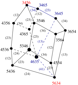
Figure 11: Bridge polytope $Br_{2,4}$: It is a characterised by vertices representing a decorated permutation of $\{1,\,2,\,3,\,4\}$, while the edges represent a transposition mapping a permutation into the other. The top decorated permutation $\{3,\,4,\,5,\,6\}$ represents the on-shell box, while the bottom one $\{5,\,6,\,3,\,4\}$ represents the identity. Any path along the edges between these two vertices represent a BCFW decomposition of the on-shell box. In blue a possible path is highlighted.

The blue path highlighted in Figure 11 represents the following sequence of BCFW bridges:

$$\begin{array}[]{ccccc}\raisebox{-45.52458pt}{\scalebox{0.25}{\includegraphics{Perm4pt.eps}}}&\overset{(34)}{\longleftrightarrow}&\raisebox{-45.52458pt}{\scalebox{0.25}{\includegraphics{Perm4ptDec34.eps}}}&\overset{\mathbb{I}}{\longleftrightarrow}&\raisebox{-45.52458pt}{\scalebox{0.25}{\includegraphics{Perm4ptDecId1.eps}}}\\ {\color[rgb]{1,0,0}\{3456\}}&{}\hfil&{\color[rgb]{0,0,1}\{3465\}}&{}\hfil&{\color[rgb]{0,0,1}\{3465\}}\\ {}\hfil&{}\hfil&{}\hfil&{}\hfil&{}\hfil\\ {}\hfil&{}\hfil&{}\hfil&{}\hfil&\left\updownarrow\right.{\mbox{\footnotesize$(23)$}}\\ {}\hfil&{}\hfil&{}\hfil&{}\hfil&{}\hfil\\ \raisebox{-45.52458pt}{\scalebox{0.25}{\includegraphics{Perm4ptDec13.eps}}}&\overset{(13)}{\longleftrightarrow}&\raisebox{-45.52458pt}{\scalebox{0.25}{\includegraphics{Perm4ptDecId2.eps}}}&\overset{\mathbb{I}}{\longleftrightarrow}&\raisebox{-45.52458pt}{\scalebox{0.25}{\includegraphics{Perm4ptDec23.eps}}}\\ {\color[rgb]{0,0,1}\{4635\}}&{}\hfil&{\color[rgb]{0,0,1}\{3645\}}&{}\hfil&{\color[rgb]{0,0,1}\{3645\}}\\ {}\hfil&{}\hfil&{}\hfil&{}\hfil&{}\hfil\\ \left\updownarrow\right.{\mbox{\footnotesize$\mathbb{I}$}}&{}\hfil&{}\hfil&{}\hfil&{}\hfil\\ {}\hfil&{}\hfil&{}\hfil&{}\hfil&{}\hfil\\ \raisebox{-45.52458pt}{\scalebox{0.25}{\includegraphics{Perm4ptDecId3.eps}}}&\overset{(41)}{\longleftrightarrow}&\raisebox{-45.52458pt}{\scalebox{0.25}{\includegraphics{Perm4ptDec41.eps}}}&{}\hfil&{}\hfil\\ {\color[rgb]{0,0,1}\{4635\}}&{}\hfil&{\color[rgb]{1,0,0}\{5634\}}&{}\hfil&{}\hfil\end{array}$$

where we displayed the trivial transformations (at step 3 and 7) which make manifest the action of the BCFW bridges.

3.2 Equivalence classes of perfectly-oriented diagrams

Having reminded how permutation works, we can now discuss how, together with the helicity flows, they define equivalence classes of perfectly-oriented diagrams. For this purpose, let us focus on the simplest example: the on-shell box (3.4). Once the labels are fixed (and we do it as in (3.4)), there is just a single equivalence class for (un-oriented) on-shell boxes and it is labelled by $\{3,\,4,\,5,\,6\}$. Let us now associate sources and sinks, and thus a set of helicity flows, to an on-shell box. Specifically, choosing $4,\,1$ as sources and $2,\,3$ as sinks, it is easy to see that both the un-decorated diagrams in the permutation $\{3,\,4,\,5,\,6\}$ enjoy the same helicity flows ${\color[rgb]{0,0,1}1}\,\longrightarrow\,{\color[rgb]{1,0,0}2}$ and ${\color[rgb]{0,0,1}4}\,\longrightarrow\,{\color[rgb]{1,0,0}3}$ along the external lines, as well as the internal $\{{\color[rgb]{0,0,1}1}{\color[rgb]{1,0,0}2}\}\,\equiv\,\{{\color[rgb]{0,0,1}4}{\color[rgb]{1,0,0}3}\}$ :

$$\raisebox{-51.21504pt}{\scalebox{0.35}{\includegraphics{4ptHelFlow6.eps}}}\qquad\Longleftrightarrow\qquad\raisebox{-51.21504pt}{\scalebox{0.35}{\includegraphics{4ptHelFlow7.eps}}}$$ (3.6)

Such an equivalence class will be denoted as $\{{\color[rgb]{0,0,1}3},\,{\color[rgb]{1,0,0}4},\,{\color[rgb]{1,0,0}5},\,{\color[rgb]{0,0,1}6}\}$. In principle, the permutation $\{3,\,4,\,5,\,6\}$ contains three more equivalence classes of this type: $\{{\color[rgb]{0,0,1}3},\,{\color[rgb]{0,0,1}4},\,{\color[rgb]{1,0,0}5},\,{\color[rgb]{1,0,0}6}\}$, $\{{\color[rgb]{1,0,0}3},\,{\color[rgb]{0,0,1}4},\,{\color[rgb]{0,0,1}5},\,{\color[rgb]{1,0,0}6}\}$ and $\{{\color[rgb]{0,0,1}3},\,{\color[rgb]{0,0,1}4},\,{\color[rgb]{1,0,0}5},\,{\color[rgb]{1,0,0}6}\}$.

Let us now take $1,\,3$ as sources and $2,\,4$ as sinks. In this case, the helicity flow structure turns out to be different, with one diagram showing external helicity flows between the adjacent boundary nodes (${\color[rgb]{0,0,1}1}\,\longrightarrow\,{\color[rgb]{1,0,0}2}$, ${\color[rgb]{1,0,0}2}\,\longleftarrow\,{\color[rgb]{0,0,1}3}$, ${\color[rgb]{0,0,1}3}\,\longrightarrow\,{\color[rgb]{1,0,0}4}$, ${\color[rgb]{1,0,0}4}\,\longleftarrow\,{\color[rgb]{0,0,1}1}$), while the other one being actually the same of the contribution of two diagrams characterised by an internal helicity loop and by just two external helicity flows

$$\raisebox{-51.21504pt}{\scalebox{0.35}{\includegraphics{4ptHelFlow1.eps}}};\qquad\raisebox{-51.21504pt}{\scalebox{0.35}{\includegraphics{4ptHelFlow2.eps}}}\>+\>\raisebox{-51.21504pt}{\scalebox{0.35}{\includegraphics{4ptHelFlow3.eps}}}$$ (3.7)

The sum above has overall the same external helicity flows, while the differently oriented internal loops should cancel in order to belong to the same equivalence class of the first diagram. This is generically not the case – it occurs just for $\mathcal{N}\,=\,3$ – and thus the above diagrams belongs to different equivalence classes, each of them containing just a single element. We denote them $({\color[rgb]{0,0,1}1},\,{\color[rgb]{1,0,0}2},\,{\color[rgb]{0,0,1}3},\,{\color[rgb]{1,0,0}4})_{\mbox{\tiny ext}}$, $({\color[rgb]{0,0,1}1},\,{\color[rgb]{1,0,0}2},\,{\color[rgb]{0,0,1}3},\,{\color[rgb]{1,0,0}4})_{\mbox{\tiny R}}$ and $({\color[rgb]{0,0,1}1},\,{\color[rgb]{1,0,0}2},\,{\color[rgb]{0,0,1}3},\,{\color[rgb]{1,0,0}4})_{\mbox{\tiny L}}$ respectively – where the subscripts ${}_{\mbox{\tiny ext}}$, ${}_{\mbox{\tiny R}}$ and ${}_{\mbox{\tiny L}}$ make reference to the fact that the related on-shell diagram has just an external, internal right-“chiral” or internal left-“chiral” helicity flow.

It is interesting to notice that the fact that the permutation contains different equivalence classes is just the statement that all of them are related by Ward identities. As we will extensively discuss in the companion paper [41], this picture will be manifest on the positive Grassmannian, where all these diagrams correspond to the same point on $G(2,4)$. In a nutshell, on-shell diagrams belonging to the same permutation are geometrically equivalent and are distinguished just by a measure which is characteristic of the particular equivalence class inside a given permutation.

For the time being, it is interesting to observe that a similar picture of the reduced on-shell diagram as a composition of BCFW bridges (i.e. adjacent transposition) holds. In particular such decomposition can still be represented as a path along the edges of a bridge polytope $Br_{k,n}$ from a given permutation (representing the diagram) to the identity. The main difference with the case discussed in Section 3.1 is due to the fact that endowing the on-shell diagrams with sources and sinks restricts the edges of the bridge polytope allowed in a path towards the identity. This restriction is due to the requirement that the sources and sinks stay fixed along the path, i.e. the boundary states have the same helicity as one acts with a BCFW bridge. As a concrete example, let us consider two different choices for the sources/sinks: $({\color[rgb]{0,0,1}1},\,{\color[rgb]{1,0,0}2},\,{\color[rgb]{1,0,0}3},\,{\color[rgb]{0,0,1}4})$, and $({\color[rgb]{0,0,1}1},\,{\color[rgb]{1,0,0}2},\,{\color[rgb]{0,0,1}3},\,{\color[rgb]{1,0,0}4})$. Beginning with the first case, there are just two paths along the edges of the bridge polytope which are consistent with the helicity flows

$$\raisebox{-51.21504pt}{\scalebox{0.33}{\includegraphics{4ptHelFlow6.eps}}}\quad\longleftrightarrow\quad\raisebox{-73.97733pt}{\scalebox{0.75}{\includegraphics{bridgehedronMPPM.eps}}}\longleftrightarrow\quad\raisebox{-51.21504pt}{\scalebox{0.33}{\includegraphics{4ptHelFlow7.eps}}}$$

where the decomposition paths are highlighted on the bridge polytope $Br_{2,4}$, in blue for the decomposition leading to the diagram on the left and in cyan for the one leading to the diagram on the right. These paths are a reflection of the physical singularities of the on-shell process they are providing the decomposition of. If one takes any of the other edges, the price one pays is the generation of a (typically helicity-dependent) Jacobian: the related BCFW bridge is of type (2.18). Each of the diagrams in the equivalence class $({\color[rgb]{0,0,1}1},\,{\color[rgb]{1,0,0}2},\,{\color[rgb]{1,0,0}3},\,{\color[rgb]{0,0,1}4})$ correspond to one of the two paths on $Br_{2,4}$.

$$\raisebox{-51.21504pt}{\scalebox{0.33}{\includegraphics{4ptHelFlow1.eps}}}\quad\longleftrightarrow\raisebox{-73.97733pt}{\scalebox{0.75}{\includegraphics{bridgehedronMPMPfin.eps}}}\longleftrightarrow\quad\raisebox{-51.21504pt}{\scalebox{0.33}{\includegraphics{4ptHelFlow2.eps}}}\quad$$

Figure 12: Bridge polytopes for perfectly-oriented diagrams. The sources and sinks are taken to be $({\color[rgb]{0,0,1}1},\,{\color[rgb]{1,0,0}2},\,{\color[rgb]{0,0,1}3},\,{\color[rgb]{1,0,0}4})$. The helicity-preserving paths provide a decomposition of either of the on-shell diagram with just external helicity flows $({\color[rgb]{0,0,1}1},\,{\color[rgb]{1,0,0}2},\,{\color[rgb]{0,0,1}3},\,{\color[rgb]{1,0,0}4})_{\mbox{\tiny ext}}$ (in blue), or of the one with the right-chiral $({\color[rgb]{0,0,1}1},\,{\color[rgb]{1,0,0}2},\,{\color[rgb]{0,0,1}3},\,{\color[rgb]{1,0,0}4})_{\mbox{\tiny R}}$ internal helicity loops (in cyan).

Let us now turn to the configuration of sources/sinks $({\color[rgb]{0,0,1}1},\,{\color[rgb]{1,0,0}2},\,{\color[rgb]{0,0,1}3},\,{\color[rgb]{1,0,0}4})$. In this case, as we saw earlier, one can distinguish three equivalence classes, each of them containing a single element. The paths corresponding to the helicity-preserving BCFW decompositions on $Br_{2,4}$ have been shown in Figure 12. Also in this case, there are just possible helicity preserving paths possible one corresponding to $({\color[rgb]{0,0,1}1},\,{\color[rgb]{1,0,0}2},\,{\color[rgb]{0,0,1}3},\,{\color[rgb]{1,0,0}4})_{\mbox{\tiny ext}}$ and the other one to $({\color[rgb]{0,0,1}1},\,{\color[rgb]{1,0,0}2},\,{\color[rgb]{0,0,1}3},\,{\color[rgb]{1,0,0}4})_{\mbox{\tiny R}}$. Let us remark that the existence of just two helicity preserving paths is just a feature of the particular choices of sinks and sources (one example where there are more decompositions allowed which respect the helicity flows is given by $({\color[rgb]{0,0,1}1},\,{\color[rgb]{0,0,1}2},\,{\color[rgb]{1,0,0}3},\,{\color[rgb]{1,0,0}4})$).

In summary, also for a decorated diagram, the bridge polytope provides its BCFW decomposition with the particular feature that just a subset of the edges are helicity preserving. If one starts from the identity and endows it with a given choice of sinks and sources, then the requirement that any transposition is decoration preserving leads along all the possible helicity preserving edges of the related bridge polytope.

3.3 More on on-shell diagrams, perfect orientations and helicity flows

In the previous sections we saw how the need of introducing new data, namely to distinguish among the coherent multiplets, led naturally to endow the diagrams with perfect orientations which are intimately related to the singularity structure of the particular on-shell process through the helicity flows that the perfect orientation itself generates.

If we abstract ourselves for a moment from our context and consider a generic un-oriented bipartite diagram which it is possible to associated a perfect orientation to, for such a perfectly oriented diagram, the inversion of a flow returns another perfect orientation as well as any other perfect orientation can be obtained from the original one by reversing the direction of a flow in the latter [47].

Such a lemma holds for our decorated diagrams as well – at the end of the day they are perfectly oriented bipartite diagrams – with a peculiarity: In our case, the flows dictated by a given perfect orientation contains information about the helicity of the states as well as the singularity structure of the on-shell process. Thus, the reversal of the direction of a helicity flow is associated to a Jacobian which transforms not trivially under the little group if the helicity flow which gets reversed involves external states, while it is helicity blind if the helicity flow is internal.

For the sake of definiteness, let us consider the fully-localised on-shell box with the configuration $({\color[rgb]{0,0,1}1},\,{\color[rgb]{1,0,0}2},\,{\color[rgb]{0,0,1}3},\,{\color[rgb]{1,0,0}4})$ for the sources and sinks. This decorate diagram shows four helicity flows, all of them involving a pair of external states. It is possible to pick any of those flows and reverse it, mapping a sink into a source and a source into a sink and generating a helicity-dependent Jacobian as in the following example:

$$\raisebox{-36.98866pt}{\scalebox{0.25}{\includegraphics{4ptHelRev1.eps}}}\quad\overset{({\color[rgb]{1,0,0}2},{\color[rgb]{0,0,1}3})}{\longrightarrow}\quad\raisebox{-36.98866pt}{\scalebox{0.25}{\includegraphics{4ptHelRev2.eps}}}\;J_{23},\qquad J_{23}\>=\>\left(\frac{\langle 1,3\rangle}{\langle 1,2\rangle}\right)^{4-\mathcal{N}}$$ (3.8)

In this way one can generate all the possible perfect orientations for the fully-localised on-shell box, i.e. all the possible configurations for the sources and sinks (helicity configuration for the external states) as well as the two diagrams with internal flow. This seven configurations can be seen as the vertices of a polytope whose edges represent the flow reversals which a Jacobian is associated to (see Figure 13).

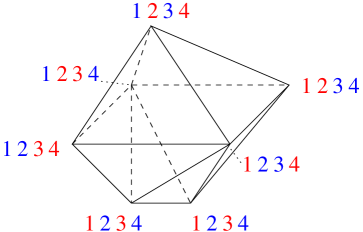
Figure 13: Polytope generated by all possible helicity-flow reversals for a fully-localised on-shell box. Each vertex of the polytope represents a given perfect orientation, while each edge represents the flow-reversal connecting them, to which a Jacobian is associated.

Notice that the edges of the polytope in Figure 13 are nothing but the Ward identities relating the tree-level four-particle amplitudes (which are all MHV). Some sort of special points are the two at the bottom of the polytope, which have the same configuration of the sources and sinks but which distinguish themselves for the clockwise/counter-clockwise internal helicity flow. The Jacobian related to the edges connecting any other vertex to them has a helicity-dependent factor of the form of $J_{23}$ in (3.8) and another one which is helicity blind and depend on the Mandelstam variables. The edge connecting these two vertices instead is the only one whose Jacobian is purely helicity blind. In (3.8) the configuration $({\color[rgb]{0,0,1}1},\,{\color[rgb]{1,0,0}2},\,{\color[rgb]{0,0,1}3},\,{\color[rgb]{1,0,0}4})$ has been taken as a reference so that, differently from the other vertices, when one goes back to it taking any path along the edges of the polytope, the overall Jacobian is the identity. In a more democratic way, one can associate to it the Jacobian factor $\langle 1,3\rangle^{-(4-\mathcal{N})}$, so that the helicity-dependent term in any Jacobian has the form $\langle{\color[rgb]{0,0,1}i},{\color[rgb]{0,0,1}j}\rangle^{-(4-\mathcal{N})}$, i.e., it depends on the sources only.

As a further comment, notice that the polytope related to the fully-localised on-shell box with the white and black nodes exchanged, can be obtained from the one in Figure 13, by contracting the two vertices labelled by $({\color[rgb]{1,0,0}1},\,{\color[rgb]{0,0,1}2},\,{\color[rgb]{1,0,0}3},\,{\color[rgb]{0,0,1}4})$ to a single one, and opening up the vertex $({\color[rgb]{0,0,1}1},\,{\color[rgb]{1,0,0}2},\,{\color[rgb]{0,0,1}3},\,{\color[rgb]{1,0,0}4})$ into two. This is a reflection of the fact that these two configurations do not satisfy a square move, while all the others do.

Finally, such a polytope can obviously be defined for any higher point on-shell process. When the helicity flows involve external states, they always show a source and a sink. This mean that any helicity-flow reversal maps a given on-shell process in another one in the same N^kMHV-sector. For $k\,=\,2$, the polytope provides with the well-known Ward identities among tree-level amplitudes as well as new ones with non-local on-shell processes. For $k\,>\,2$, the helicity-flow reversals do not in general map an amplitude into another amplitude, so that the polytopes typically describe relation among individual on-shell processes.

4 On-shell processes and scattering amplitudes

So far we have been discussing generic on-shell processes in order to illustrate some important features of the decorated diagrammatics as well as how special points can be related to each other. Let us now turn to actual scattering amplitudes. The objects of interest are actually the integrands in the perturbative expansion. The on-shell diagrammatics then generates an expansion in terms of $4L$-forms which, upon (regulated) integration on the Lorentz real sheet, returns the physical amplitude. Actually, the on-shell diagrammatics provides an object from which a great deal of physical information can be extracted, depending on the path/manifold on which one integrates it. The general form can be written as

$$\mathcal{M}_{n}(\{\lambda^{\mbox{\tiny$(i)$}},\,\tilde{\lambda}^{\mbox{\tiny$(i)$}};\,h_{i}\})\>=\>\sum_{L=0}^{\infty}\mathcal{M}_{n}^{\mbox{\tiny$(L)$}}(\{\lambda^{\mbox{\tiny$(i)$}},\,\tilde{\lambda}^{\mbox{\tiny$(i)$}};\,h_{i}\},\,\{z_{l}\})\bigwedge_{l=1}^{4L}dz_{l},$$ (4.1)

where the expansion coefficients $\mathcal{M}_{n}^{\mbox{\tiny$(L)$}}(\{\lambda^{\mbox{\tiny$(i)$}},\,\tilde{\lambda}^{\mbox{\tiny$(i)$}};\,h_{i}\},\,\{z_{l}\})$ are rational function of both the Lorentz invariant combination of the spinors and of the parameters $\{z_{l}\}$. It is easy to see that the $L=0$ term is a $0$-form and, therefore, receives contributions from fully localised on-shell diagrams, while for $L\,\geq\,1$ the on-shell diagrams must have $4L$ degrees of freedom left unfixed (for a given $L$) and these terms can generate branch cuts upon integration of such degrees of freedom over a suitable manifold. The $L$-th order terms is then the seed from which the $L$-loop amplitude can be extracted (upon a suitable integration).

In the case of $\mathcal{N}\,=\,4$ SYM it was shown that scattering amplitudes satisfy an all-loop recursion relation [17], which can be understood as the solution of a differential equation encoding all the singularities of the amplitudes at a given loop $L$, which gets integrated via a BCFW bridge [20]:

$$\begin{split}&\partial\left[\raisebox{-42.67912pt}{\scalebox{0.55}{\includegraphics{N4SYMrrLHS.eps}}}\right]\>=\>\sum_{L,\,R}\;\raisebox{-28.45274pt}{\scalebox{0.55}{\includegraphics{N4SYMrrRHS1.eps}}}+\sum_{k}\raisebox{-36.98866pt}{\scalebox{0.55}{\includegraphics{N4SYMrrRHS2.eps}}}\\ &\hskip 199.16928pt\Downarrow\\ &\hskip 14.22636pt\raisebox{-42.67912pt}{\scalebox{0.55}{\includegraphics{N4SYMrrLHS.eps}}}\>=\>\sum_{k\in\mathcal{P}}\;\mathcal{I}_{k}\raisebox{-65.44142pt}{\scalebox{0.55}{\includegraphics{N4SYMrrRHS3.eps}}}\mathcal{J}_{k}+\raisebox{-71.13188pt}{\scalebox{0.55}{\includegraphics{N4SYMrrRHS4.eps}}}\end{split}$$ (4.2)

where the first term in the first line indicate all the possible factorisation channels, with the sub-amplitudes labelled by $L$ and $R$ being $l$- and $(L-l)$-loop amplitudes with $n_{\mbox{\tiny$L$}}+1$ and $n_{\mbox{\tiny$R$}}+1$ external states ($n_{\mbox{\tiny$L$}}+n_{\mbox{\tiny$R$}}\,=\,n$), while the second term represents the forward-limit of a $(L-1)$-loop amplitude with $n+2$ external states [40]. In the second line, the BCFW bridge select a sub-set of the singularities, with $\mathcal{P}$ indicating the set of factorisation channels with the particles in the bridge belonging to different sub-amplitudes, and $\mathcal{I}_{k}$ and $\mathcal{J}_{k}$ indicating a partition of all the external particles but the ones labelled by $i$ and $i+1$ which respects colour ordering ($\mathcal{I}_{k}\,\cup\,\mathcal{J}_{k}\>=\>\{1,\ldots,n\}\,\backslash\,\{i,i+1\}$, with dim$\{\mathcal{I}_{k}\,\cup\,\mathcal{J}_{k}\}\,=\,n-2$). The validity of the recursive relation (4.2) has a very neat fully-diagrammatic proof [20].

In the less/no-supersymmetric case the story turns out to be similar but not quite, due to the presence of additional structures than the simple $d\log{\zeta}$ which characterises the maximally supersymmetric case. The first concern which arises is related to the definition itself of the integrand due to the possible presence of external bubbles and external tadpoles. However, for $\mathcal{N}\,\geq\,1$ it has been shown that the sum over the full multiplet(s) makes these contributions vanish [40] and, thus, the object integrand stays well-defined, with the loop singularities – i.e. the ones corresponding to a loop-degree-of-freedom dependent propagator going on-shell – which still can be interpreted as a forward limit of a lower-loop amplitude. Furthermore, for $\mathcal{N}\,\geq\,1$, the amplitudes are cut-constructible [57, 58], which suggests the validity of a loop recursive structure. More subtle is the $\mathcal{N}\,=\,0$ case.

4.1 Fully localised diagrams: The tree level structure

Let us begin with considering just fully-localised on-shell diagrams. The validity of the recursion relations of the amplitude under a particular BCFW bridging can be shown diagrammatically along the same lines of the diagrammatic proof [20] that all the correct factorisation channels are contained in (4.2).

The starting point is given by the two sets of four-particle amplitudes for which the factorisation channels are manifest and follow the helicity lines

$$\begin{split}&\partial\left[\raisebox{-34.14322pt}{\scalebox{0.25}{\includegraphics{4ptHelFlow1.eps}}}\right]\>=\>\raisebox{-28.45274pt}{\scalebox{0.25}{\includegraphics{4ptSing2a.eps}}}\;+\;\raisebox{-28.45274pt}{\scalebox{0.25}{\includegraphics{4ptSing2b.eps}}}\;+\;\raisebox{-25.6073pt}{\scalebox{0.25}{\includegraphics{4ptSing2c.eps}}}\;+\;\raisebox{-25.6073pt}{\scalebox{0.25}{\includegraphics{4ptSing2d.eps}}}\\ &\partial\left[\raisebox{-34.14322pt}{\scalebox{0.25}{\includegraphics{4ptHelFlow4.eps}}}\right]\>=\>\raisebox{-28.45274pt}{\scalebox{0.25}{\includegraphics{4ptSing3a.eps}}}\;+\;\raisebox{-28.45274pt}{\scalebox{0.25}{\includegraphics{4ptSing3d.eps}}}\;+\;\raisebox{-25.6073pt}{\scalebox{0.25}{\includegraphics{4ptSing3c.eps}}}\end{split}$$ (4.3)

Notice that the differential equations above are generally integrated to return a scattering amplitude just by those BCFW bridges which do not create internal helicity loops and preserve the helicity flows on the right-hand-side of (4.3). A special case is provided by the $\mathcal{N}\,=\,3$ SYM for which the sum of the two diagrams with internal loops also provides the correct tree amplitudes. As we mentioned earlier, this is the consequence of the fact that, for $\mathcal{N}\,=\,3$, an internal helicity loop corresponds to the presence of a simple pole rather than a multiple one as for $\mathcal{N}\,\leq\,2$, which disappears upon summing between the two diagrams with differently-oriented helicity-loops.

Then, one can assume as induction hypothesis the following relation for the $n$-particle amplitude:

$$\begin{split}\raisebox{-31.2982pt}{\scalebox{0.45}{\includegraphics{N4SYMrrLHS.eps}}}\>&=\>\sum_{k\in\mathcal{P}}\;\mathcal{I}_{k}\raisebox{-54.06006pt}{\scalebox{0.45}{\includegraphics{RRmp.eps}}}\mathcal{J}_{k}\>=\>\sum_{k\in\tilde{\mathcal{P}}}\;\tilde{\mathcal{I}}_{k}\raisebox{-56.9055pt}{\scalebox{0.45}{\includegraphics{RRmm.eps}}}\tilde{\mathcal{J}}_{k}\\ &=\>\sum_{k\in\hat{\mathcal{P}}}\;\hat{\mathcal{I}}_{k}\raisebox{-56.9055pt}{\scalebox{0.45}{\includegraphics{RRpp.eps}}}\hat{\mathcal{J}}_{k}\end{split}$$ (4.4)

where $\mathcal{I}_{k}\,\cup\,\mathcal{J}_{k}\,=\,\{1,\,\ldots,\,n\}\,\backslash\,\{i,\,i+1\}$, $\tilde{\mathcal{I}}_{k}\,\cup\,\tilde{\mathcal{J}}_{k}\,=\,\{1,\,\ldots,\,n\}\,\backslash\,\{j,\,j+1\}$, $\hat{\mathcal{I}}_{k}\,\cup\,\hat{\mathcal{J}}_{k}\,=\,\{1,\,\ldots,\,n\}\,\backslash\,\{m,\,m+1\}$, and the BCFW bridge needs to be chosen in such a way that no helicity loop is generated in the interior of the diagram. With this assumption, one now need to show that the above formula is valid for a higher number of particles, i.e. that for higher number of particles it contains all and only the correct collinear and multi-particle factorisation channels.

Actually, the full discussion follows closely the one for the maximally supersymmetric case, given that it is part of our inductive assumption the way that a BCFW bridge can be taken. This means the helicity flows are always preserved and at no stage internal helicity loop can be generated.

The representations (4.4) make all those channels having the particle pairs $\{i,\,i+1\}$, $\{j,\,j+1\}$ and $\{m,\,m+1\}$ on different sub-amplitudes manifest and, thus, these factorisation are trivially included.

Let us consider the factorisation channel $\mathcal{K}$, where $\mathcal{K}$ is a set of external states such that either $\mathcal{K}\>\subset\>\mathcal{I}_{k}$ or $\mathcal{K}\>\subset\>\mathcal{J}_{k}$. In this case, one has two classes of terms characterised by two sub-amplitudes are bridged by the initial bridge itself. The sum over these two classes of terms because of our induction hypothesis provides a single full-fledge sub-amplitude. Explicitly:

$$\begin{array}[]{ccc}\mathcal{I}_{k}\raisebox{-45.52458pt}{\scalebox{0.4}{\includegraphics{RRmp.eps}}}\mathcal{J}_{k}&{}\hfil&\raisebox{-45.52458pt}{\scalebox{0.4}{\includegraphics{RRfactorfin.eps}}}\\ {}\hfil&{}\hfil&{}\hfil\\ \downarrow&{}\hfil&\Uparrow\\ {}\hfil&{}\hfil&{}\hfil\\ \sum_{k^{\prime}}\begin{array}[]{l}\vspace{.4cm}\hskip 5.69046pt\mathcal{K}\\ \phantom{\mathcal{K}}\\ \mathcal{I}_{k^{\prime}}^{\mbox{\tiny$(a)$}}\end{array}\raisebox{-45.52458pt}{\scalebox{0.4}{\includegraphics{RRfactor1.eps}}}\;\mathcal{J}_{k^{\prime}}&+&\sum_{k^{\prime\prime}}\mathcal{I}_{k^{\prime\prime}}\raisebox{-45.52458pt}{\scalebox{0.4}{\includegraphics{RRfactor2.eps}}}\begin{array}[]{l}\vspace{1cm}\mathcal{K}\\ \phantom{\mathcal{K}}\\ \vspace{.2cm}\mathcal{J}_{k^{\prime\prime}}^{\mbox{\tiny$(b)$}}\end{array}\end{array}$$ (4.5)

As far as the factorisation in the $(i,\,i+1)$-channel is concerned, the diagrammatics offers a very straightforward way to show that it is also contained in the recursive formula. Notice that for each of the two possible complex factorisations, there is just a single diagram which can contribute, which is characterised by a three-particle amplitude in the factorisation channel. For the sake of concreteness, let us fix the sink/sources for the states in the bridge to be $({\color[rgb]{1,0,0}i},\,{\color[rgb]{0,0,1}i+1})$, then irrespectively of whether the three-particle amplitude which connects particle $i$ and $i+1$ has a sink or sources, there are always well defined helicity flows among the external states:

$$\begin{array}[]{ccc}\raisebox{-45.52458pt}{\scalebox{0.4}{\includegraphics{RRcoll.eps}}}&\qquad\longrightarrow&\raisebox{-45.52458pt}{\scalebox{0.4}{\includegraphics{RRcollb.eps}}}\\ {}\hfil&{}\hfil&{}\hfil\\ \raisebox{-45.52458pt}{\scalebox{0.4}{\includegraphics{RRcoll2.eps}}}&\qquad\longrightarrow&\quad\raisebox{-45.52458pt}{\scalebox{0.4}{\includegraphics{RRcoll2b.eps}}}\end{array}$$ (4.6)

The very same argument applies when the three-particle amplitude is $\mathcal{M}_{3}^{\mbox{\tiny$(1)$}}$. These two possibilities correspond to the two possible complex factorisation channels that one can have in a collinear limit [59, 37]. Indeed, not necessarily an amplitude must factorise under both. However, are exactly the helicity flows which tell us whether both are allowed or just one of them.

Finally, there are further poles that in principle can arise and which are non-local. However they always appear in pairs and they cancel, leaving just the physical singularities. This can be easily see diagrammatically as follows

$$\raisebox{-45.52458pt}{\scalebox{0.4}{\includegraphics{RRmp.eps}}}\quad\Longrightarrow\quad\raisebox{-45.52458pt}{\scalebox{0.4}{\includegraphics{RRmpNL1.eps}}}\quad+\quad\raisebox{-45.52458pt}{\scalebox{0.4}{\includegraphics{RRmpNL2.eps}}}$$ (4.7)

where the green line indicates the non-local pole, which in the first diagram is generated from the sub-amplitude on the left while in the second diagram from the sub-amplitude on the right.

A couple of comments are now in order. Our starting point – i.e. the four-point relations in which all the factorisation channels are manifest (4.3) – shows just external helicity flows. As we already discussed, in the case the other possible relation is considered, there are two contributions each of which show two helicity flows in a single channel as well as an internal helicity loop. This internal helicity loop corresponds to a further singularity which disappears upon their summation just for $\mathcal{N}\,=\,3$. Except that for this particular theory, these diagrams provide an object with a different singularity structure than a scattering amplitude and, therefore, they cannot be used as a starting point for an inductive argument. Furthermore, their presence at any step of the inductive procedure would invalidate the proof. However, as stated earlier, they can never arise: This is a consequence of the fact that the inductive hypothesis just contain full-fledge sub-amplitudes which themselves can be just expressed in terms of diagrams with no internal helicity loop!

4.1.1 On the boundary terms

It is instructive to further explore the fully localised diagrams by comparing the different ones with a given external helicity configuration.

Given a fixed helicity configuration for the external states and singled out two of them, we define as boundary term the difference between the two ways of integrating the on-shell differential equation for the amplitude. If this boundary term is non-vanishing, a singularity has been missed by at least one of the BCFW bridge. In the case of planar gauge theories, such a boundary term is related just to a specific BCFW bridge.

As a starting point, let us consider the four-particle amplitudes both in the $(-,-,+,+)$ and $(-,+,-,+)$ helicity configurations. The boundary terms $\Delta\mathcal{M}_{4}^{\mbox{\tiny tree}}$ are then given by

$$\begin{split}&\Delta\mathcal{M}_{4}^{\mbox{\tiny tree}}(-,-,+,+)\>=\>\raisebox{-31.2982pt}{\scalebox{0.25}{\includegraphics{4ptHelFlow5.eps}}}-\raisebox{-31.2982pt}{\scalebox{0.25}{\includegraphics{4ptHelFlow4.eps}}}\\ &\Delta\mathcal{M}_{4}^{\mbox{\tiny tree}}(-,+,-,+)\>=\>\raisebox{-31.2982pt}{\scalebox{0.25}{\includegraphics{4ptHelFlow1.eps}}}-\raisebox{-31.2982pt}{\scalebox{0.25}{\includegraphics{4ptHelFlow2.eps}}}-\raisebox{-31.2982pt}{\scalebox{0.25}{\includegraphics{4ptHelFlow3.eps}}}\end{split}$$ (4.8)

and they can also be seen as a measure of the inequivalence of a square move. As we saw earlier, the two terms in the first line of (4.8) are actually always (i.e. for any $\mathcal{N}$) equal – as a quick analysis of the helicity flows shows. As far as the boundary term in the second line is concerned, while the first diagram shows all the complex factorisation in both the $s$- and $t$-channels, the second and third diagrams shows the two complex factorisations in just one channel ($t$ and $s$, respectively) while the presence of oriented internal helicity loops reveal the presence of a extra poles

$$\begin{split}\Delta\mathcal{M}_{4}^{\mbox{\tiny tree}}(-,+,-,+)\>&=\>\mathcal{M}_{4}^{\mbox{\tiny tree}}(-,+,-,+)(-1)^{4-\mathcal{N}}\sum_{k=1}^{3-\mathcal{N}}\begin{pmatrix}4-\mathcal{N}\\ k\end{pmatrix}\frac{s^{k}t^{4-\mathcal{N}-k}}{u^{4-\mathcal{N}}}\>=\\ &=\>\mathcal{M}_{4}^{\mbox{\tiny tree}}(-,+,-,+)\left[\varepsilon_{\mathcal{N},3}(4-\mathcal{N})\frac{st}{u^{2}}-\delta_{\mathcal{N},0}2\frac{s^{2}t^{2}}{u^{4}}\right].\end{split}$$ (4.9)

The $\mathcal{N}\,=\,3$ case is the only one in which the poles related to the internal loops are simple pole and cancel when the two contributions get summed. For $\mathcal{N}\,\leq\,2$, these poles become higher order a no cancellation occurs. More precisely, the poles do not disappear, however, while the theory is supersymmetric, cancellations occur in such a way that just double poles appear. In particular, this boundary term appears to be universal, up to an overall constant, in its kinematic structure (i.e. it does not depend on $\mathcal{N}$ as long as $\mathcal{N}\,\leq\,2$). Just for $\mathcal{N}\,=\,0$, an extra term appears showing a fourth order pole.

If we instead look at higher point localised diagrams, it is interesting to notice that in the MHV sector the boundary term defined through diagrams containing at most one internal helicity loop can be constructed from the one we just discussed by adding inverse soft factors

$$\Delta\mathcal{M}_{n}^{\mbox{\tiny tree}}(1^{-},2^{+},3^{-},4^{+},\ldots,n^{+})\>=\>\Delta\mathcal{M}_{4}^{\mbox{\tiny tree}}(1^{-},2^{+},3^{-},n^{+})\otimes\bigotimes_{k=0}^{n-5}\mbox{Soft}_{+}^{\mbox{\tiny tree}}(n-1-k),$$ (4.10)

with $\mbox{Soft}_{+}^{\mbox{\tiny tree}}(n-1-k)$ being the soft factor for the positive helicity multiplet labelled by $n-1-k$, i.e. three-particle amplitude suitably attached to the lower-point amplitude. This is just a consequence of the fact that the full-fledge amplitudes in the MHV sector can be constructed by inverse soft procedure (they are always given by a single on-shell diagram irrespectively of the number of external states), as well as in the definition of $\Delta\mathcal{M}_{n}$ diagrams with at most one internal helicity loop are considered. Exactly the same construction holds for the $\bar{\mbox{MHV}}$ sector

$$\Delta\mathcal{M}_{n}^{\mbox{\tiny tree}}(1^{-},2^{+},3^{-},4^{+},5^{-}\ldots,n^{-})\>=\>\Delta\mathcal{M}_{4}^{\mbox{\tiny tree}}(1^{-},2^{+},3^{-},4^{+})\otimes\bigotimes_{k=5}^{n}\mbox{Soft}_{-}^{\mbox{\tiny tree}}(k).$$ (4.11)

4.2 On-shell $1$-forms and $2$-forms: the one-loop structure

Let us now turn to more interesting diagrams, beginning with those ones which can be obtained from the localised diagrams via the application of a BCFW bridge, as in Figure 10. This is the same class of diagrams we discussed in Section 2.6, where we analysed its pole structure and emphasised mostly the tree level information. Actually, the very same information is directly connected with the loop structure of the theory. Specifically, this class of diagram corresponds, in a more standard language, to a triple cut of a one-loop amplitude. More precisely, it corresponds to one of the two families of solutions of the triple-cut equations. Let us analyse it in some detail. The one-form $\mathcal{M}_{4}^{\mbox{\tiny$(1)$}}(z)$ generated by BCFW-bridging the tree-level four-particle amplitude $\mathcal{M}_{4}(-,+,-,+)$ can be written as

$$\begin{split}\mathcal{M}_{4}^{\mbox{\tiny$(1)$}}(z)\>&=\>\mathcal{M}_{4}^{\mbox{\tiny tree}}\frac{dz_{12}}{z_{12}\left(1+\frac{\langle 4,2\rangle}{\langle 4,1\rangle}z_{12}\right)}\left[\left(1+\frac{\langle 2,3\rangle}{\langle 1,3\rangle}z_{12}\right)^{4-\mathcal{N}}+\left(-\frac{\langle 2,3\rangle}{\langle 1,3\rangle}z_{12}\right)^{4-\mathcal{N}}\right]\>=\\ &=\>\mathcal{M}_{4}^{\mbox{\tiny tree}}\frac{dz_{34}}{z_{34}\left(1+\frac{\langle 3,1\rangle}{\langle 4,1\rangle}z_{34}\right)}\left[\frac{\left(-\frac{s}{u}\right)^{4-\mathcal{N}}+\left(-\frac{t}{u}\right)^{4-\mathcal{N}}\left(1+\frac{\langle 3,1\rangle}{\langle 4,1\rangle}z_{34}\right)^{4-\mathcal{N}}}{\left(1+\frac{\langle 2,3\rangle}{\langle 2,4\rangle}z_{34}\right)^{4-\mathcal{N}}}\right],\end{split}$$ (4.12)

where the second line represents the parametrisation of this diagram looked as a BCFW bridge of the two helicity loop four-particle diagrams. This on-shell one-form shows three singular points: $z_{12}\,=\,0,\,\infty,\,-\langle 4,1\rangle/\langle 4,2\rangle$, or, equivalently in the $z_{34}$ parametrisation, $z_{34}\,=\,0,\,-\langle 2,4\rangle/\langle 2,4\rangle,\,-\langle 4,1\rangle/\langle 4,2\rangle$. As mentioned in Section 2.6, the integration on a $T^{1}$ around the points $z_{12}\,=\,0$ ($z_{34}\,=\,-\langle 4,1\rangle/\langle 4,2\rangle$) and $z_{12}\,=\,-\langle 4,1\rangle/\langle 4,2\rangle$ ($z_{34}\,=\,0$) returns the two leading singularities, i.e. this integration localises the on-shell form on diagrams which has either external helicity flows only or internal helicity loops. The one-form (4.12) shows also a multiple pole which is at infinity in the $z_{12}$ parametrisation or at finite location in the $z_{34}$-one. The related residue is nothing but the boundary term of the tree-level amplitude we started with, but it also provides the coefficient of the scalar triangle in the $(1,2)$-channel.

Let us now turn to the following on-shell two-forms with four external states:

$$\begin{split}\mathcal{M}^{\mbox{\tiny$(2)$}}_{4}(\zeta)\>&=\>\raisebox{-35.56593pt}{\scalebox{0.3}{\includegraphics{DoubleCut1.eps}}}+\raisebox{-35.56593pt}{\scalebox{0.3}{\includegraphics{DoubleCut2.eps}}}\>=\\ &=\>\mathcal{M}_{4}^{\mbox{\tiny tree}}\,\frac{d\zeta_{12}}{\zeta_{12}}\wedge\frac{d\zeta_{34}}{\zeta_{34}}\frac{\left(-\frac{t}{u}\right)^{4-\mathcal{N}}+\left(-\frac{s}{u}\right)^{4-\mathcal{N}}\left(1-\zeta_{12}\right)^{4-\mathcal{N}}\left(1-\zeta_{34}\right)^{4-\mathcal{N}}}{\left[-\frac{t}{u}-\frac{s}{u}\left(1-\zeta_{12}\right)\left(1-\zeta_{34}\right)\right]^{4-\mathcal{N}}},\end{split}$$ (4.13)

which can be looked at as two BCFW bridges applied onto the two chiral boxes, i.e. one of the two leading singularities, with $\zeta_{12}$ and $\zeta_{34}$ being the free degrees of freedom induced by the bridging in the $(1,2)$- and $(3,4)$-channel respectively. The helicity flows highlight the equivalence operation which are allowed: while the second contribution (4.13) is rigidly fixed (the helicity flows among the external states are all outer to the diagram), in the first one, it is possible to apply first a square move on each of the most external boxes and perform a bubble deletion on clockwise on-shell bubbles. The presence of such on-shell bubble after equivalence operations can be predicted because of the presence of the clockwise chiral box. In any case, in both terms, the presence of the chiral boxes implies the presence of a multiple pole. As usual, a big deal of physical information can be extracted from the (multivariate) residues of the singularities.

Differently from the case analysed earlier, now the integration contours are $2$-cycles in $\mathbb{CP}^{2}$ and, in principle, the multivariate residues can depend on the ordering in which the integration is performed.

Using the homogeneous coordinates $[w_{0},\,w_{12},\,w_{34}]$ for $\mathbb{CP}^{2}$, which are related to our local coordinates $(\zeta_{12},\,\zeta_{34})\,\in\,\mathbb{C}^{2}$ via the map $[w_{0},\,w_{12},\,w_{34}]\,\longrightarrow\,[\zeta_{12}(w),\,\zeta_{34}(w)]$ with $\zeta_{i,i+1}\,=\,w_{i,i+1}/w_{0}$, the two-form $\mathcal{M}_{4}^{\mbox{\tiny$(2)$}}$ in (4.13) is well-defined everywhere except on the following hypersurfaces:

$$w_{0}\,=\,0,\quad w_{12}\,=\,0,\quad w_{34}\,=\,0,\quad-\frac{s}{u}(w_{0}-w_{12})(w_{0}-w_{34})-\frac{t}{u}w_{0}^{2}\,=\,0,$$ (4.14)

with $w_{0}\,=\,0$ being the point at infinity. The singularities can be seen as the discrete set of points given by two divisors defined out of the hypersurfaces (4.14). Let us begin with defining the following divisors

$$D_{1}\,=\,\left\{w_{0}w_{12}\,=\,0\right\}\;\mbox{and}\;D_{2}\,=\,\left\{w_{34}\left(-\frac{s}{u}(w_{0}-w_{12})(w_{0}-w_{34})-\frac{t}{u}w_{0}^{2}\right)^{4-\mathcal{N}}\,=\,0\,\right\}.$$ (4.15)

The intersection $D_{1}\,\cap\,D_{2}$ is a discrete set whose elements are singular points for the two-form under analysis:

$$D_{1}\,\cap\,D_{2}\>=\>\left\{\left.[w_{0},\,w_{12},\,w_{34}]\,\in\,\mathbb{CP}^{2}\,\right|\,[0,\,1,\,0],\,[1,\,0,\,0],\,\left[1,\,0,\,-\frac{u}{s}\right]\right\}.$$ (4.16)

Such a set contains one point, the first one in (4.16), at infinity and the origin as single poles, as well as a further point (the third one) as a multiple pole.

The two-form (4.13) is invariant under the label exchange $(1,2)\,\longleftrightarrow\,(3.4)$, so that two more divisors, and therefore their intersection, is obtained from (4.15) and (4.16) by such a label exchange.

The two intersections so defined expose two poles at infinity, the origin and two multiple poles. It is not difficult to see that the residue of both poles at infinity corresponds to the leading singularity with no internal helicity loop. In the same way, the residues at the origin and at the multiple pole respectively provides the other leading singularity and the scalar triangle coefficient. Furthermore, the global residue theorem [61] implies that the sum of the residues of the two-form for each divisor intersection above vanishes, i.e. the global residue theorem relates the leading singularities and (one) coefficient of the scalar triangle, returning the tree level relations discussed in the previous subsection.

A further choice for the divisors can be done by taking

$$D^{\prime}_{1}\,=\,\left\{w_{12}\,w_{34}\,=\,0\right\}\;\mbox{and}\;D^{\prime}_{2}\,=\,\left\{w_{0}\left(-\frac{s}{u}(w_{0}-w_{12})(w_{0}-w_{34})-\frac{t}{u}w_{0}^{2}\right)^{4-\mathcal{N}}\,=\,0\,\right\},$$ (4.17)

whose intersection is made of two points at infinity and two multiple poles

$$D^{\prime}_{1}\,\cap\,D^{\prime}_{2}\>=\>\left\{\left.[w_{0},\,w_{12},\,w_{34}]\,\in\,\mathbb{CP}^{2}\,\right|\,[0,\,0,\,1],\,[0,\,1,\,0],\,\left[1,\,0,\,-\frac{u}{s}\right],\,\left[1,\,-\frac{u}{s},\,0\right]\right\}.$$ (4.18)

The residues at these points are equal in pairs and, when applying the global residue theorem, they acquire opposite sign so that the overall sign over the residues for this intersection is also zero. However, contrarily to the previous case no interesting physical relation is encoded.

The $2$-cycles described above are also straightforward to analyse directly in the local coordinates $(\zeta_{12},\,\zeta_{34})$ in (4.13). In particular:

• $\gamma_{\mbox{\tiny LS}}^{\mbox{\tiny$(1)$}}\,=\,\{(\zeta_{23},\,\zeta_{41})\,\in\hat{\mathbb{C}}^{2}\,|\,\zeta_{23}\,=\,0,\,\zeta_{41}\,=\,0\}$ returns one of the leading singularities:

  $$\begin{split}\oint_{\gamma_{\mbox{\tiny LS}}^{\mbox{\tiny$(1)$}}}\,\mathcal{M}_{4}^{\mbox{\tiny$(2)$}}(\zeta)\>&=\>\raisebox{-35.56593pt}{\scalebox{0.25}{\includegraphics{4ptHelFlow2.eps}}}\quad+\>\raisebox{-35.56593pt}{\scalebox{0.25}{\includegraphics{4ptHelFlow3.eps}}}\qquad=\\ &=\>\mathcal{M}_{4}^{\mbox{\tiny tree}}\left[\left(-\frac{t}{u}\right)^{4-\mathcal{N}}+\left(-\frac{s}{u}\right)^{4-\mathcal{N}}\right]\end{split}$$ (4.19)

• $\gamma_{\mbox{\tiny LS}}^{\mbox{\tiny$(2)$}}\,=\,\{(\zeta_{23},\,\zeta_{41})\,\in\hat{\mathbb{C}}^{2}\,|\,\zeta_{23}\,=\,\infty,\,\zeta_{41}\,=\,\infty\}$ returns the second leading singularity:

  $$\oint_{\gamma_{\mbox{\tiny LS}}^{\mbox{\tiny$(2)$}}}\,\mathcal{M}_{4}^{\mbox{\tiny$(2)$}}(\zeta)\>=\>\raisebox{-35.56593pt}{\scalebox{0.25}{\includegraphics{4ptHelFlow1.eps}}}\>=\>\mathcal{M}_{4}^{\mbox{\tiny tree}}.$$ (4.20)

  Notice that both in this case and in the previous one, the integration order does not matter.

• $\gamma_{\mbox{\tiny$\triangle$}}^{\mbox{\tiny$(1)$}}\,=\,\{(\zeta_{23},\,\zeta_{41})\,\in\hat{\mathbb{C}}^{2}\,|\,\zeta_{23}\,=\,0,\,\zeta_{41}\,=\,-u/t;\>\zeta_{41}\,\succ\,\zeta_{23}\}$, where $\zeta_{41}\,\succ\,\zeta_{23}$ establishes a lexicographical order. Actually, one can integrate over $\zeta_{41}$ first by taking $\zeta_{23}$ fixed and then integrating over $\zeta_{23}$: The result stays unchanged and is the coefficient of a triangle integral in the $t$-channel.

  $$\begin{split}\oint_{\gamma_{\triangle}^{\mbox{\tiny$(1)$}}}\mathcal{M}_{4}^{\mbox{\tiny$(2)$}}(\zeta)\>&=\>\raisebox{-35.56593pt}{\scalebox{0.3}{\includegraphics{DoubleCutTriang.eps}}}+\raisebox{-35.56593pt}{\scalebox{0.3}{\includegraphics{DoubleCutTriang2.eps}}}\>=\\ &=\mathcal{M}_{4}^{\mbox{\tiny tree}}\left[\varepsilon_{\mathcal{N},3}(4-\mathcal{N})\frac{st}{u^{2}}-\delta_{\mathcal{N},0}2\frac{s^{2}t^{2}}{u^{4}}\right]\end{split}$$ (4.21)

• $\gamma_{\mbox{\tiny$\triangle$}}^{\mbox{\tiny$(2)$}}\,=\,\{(\zeta_{23},\,\zeta_{41})\,\in\hat{\mathbb{C}}^{2}\,|\,\zeta_{41}\,=\,0,\,\zeta_{23}\,=\,-u/t;\>\zeta_{23}\,\succ\,\zeta_{41}\}$ returns again the coefficient of a triangle integral – the same discussion above applies up to the label exchange $23\,\longleftrightarrow\,41$.

The extraction of the bubble coefficient is a bit more subtle and it is related to the multiple pole defined by the last hypersurface in (4.14) with no intersection with any of the other hypersurfaces.

Thus, the residues of the poles in the $2$-form (4.13) encodes all the physical information contained in a double cut. In order to understand how the differences between the supersymmetric theories and pure Yang-Mills arise, it is instructive to rewrite (4.13) as follows:

$$\begin{split}\mathcal{M}_{4}^{\mbox{\tiny$(2)$}}(\zeta)\>&=\>\frac{d\zeta_{12}}{\zeta_{12}}\wedge\frac{d\zeta_{34}}{\zeta_{34}}\left\{1-\varepsilon_{\mathcal{N},3}\left[\frac{(4-\mathcal{N})\left(-\frac{t}{u}\right)}{-\frac{t}{u}-\frac{s}{u}\left(1-\zeta_{12}\right)\left(1-\zeta_{34}\right)}-\right.\right.\\ &\left.\left.-\frac{(4-\mathcal{N})\left(-\frac{t}{u}\right)^{2}}{\left[-\frac{t}{u}-\frac{s}{u}\left(1-\zeta_{12}\right)\left(1-\zeta_{34}\right)\right]^{2}}\right]+\delta_{\mathcal{N},0}\left[\frac{2\left(-\frac{t}{u}\right)^{2}\left(-\frac{s}{u}\right)}{\left[-\frac{t}{u}-\frac{s}{u}\left(1-\zeta_{12}\right)\left(1-\zeta_{34}\right)\right]^{3}}-\right.\right.\\ &-\left.\left.\frac{2\left(-\frac{t}{u}\right)^{3}\left(-\frac{s}{u}\right)}{\left[-\frac{t}{u}-\frac{s}{u}\left(1-\zeta_{12}\right)\left(1-\zeta_{34}\right)\right]^{4}}\right]\right\}.\end{split}$$ (4.22)

The expression above makes manifest that the difference in between the structure of supersymmetric case and pure Yang-Mills is encoded in the different behaviour with the composite pole, which is a direct consequence of the different structure in the boundary terms discussed in Section 4.1.1.

4.3 Forward amplitudes and singularities

One of the key observations which allowed to prove the all-loop integrand BCFW recursion relation in $\mathcal{N}\,=\,4$ SYM has been the correct and non-ambiguous interpretation of the singularities characteristic of the loop amplitudes. Specifically, when a BCFW deformation of a loop amplitude is performed, also the loop propagators acquire a BCFW-parameter dependence and the related residues are given by a single cut. In general, single cuts can be a highly ill-defined procedure, except for the $\mathcal{N}\,\geq\,1$ massless supersymmetric planar gauge theories and the $\mathcal{N}\,\geq\,2$ massive ones [40]. In those theories, the residues of this singularity are interpreted as forward amplitudes of one perturbative order less.

In this section, we analyse the one-loop four-particle case in some detail, including the non-supersymmetric case. The general claim is that the on-shell diagrammatics provides a natural definition for the forward limit also in those cases where the limit is singular, such as $\mathcal{N}\,=\,0$ Yang-Mills, where some subtleties need to be taken care of. As a first step, we consider the following quantity

$$\mathcal{M}_{4}^{\mbox{\tiny$(1)$}}\>=\>\raisebox{-51.21504pt}{\scalebox{0.4}{\includegraphics{ForwardInt.eps}}}\>=\>\frac{dz_{41}}{z_{41}}\wedge\frac{d^{2}\lambda^{\mbox{\tiny$(AB)$}}d^{2}\tilde{\lambda}^{\mbox{\tiny$(AB)$}}}{\mbox{Vol}\{GL(1)\}}\,\mathcal{M}_{6}^{\mbox{\tiny tree}}({\color[rgb]{1,0,0}AB},{\color[rgb]{1,0,0}-AB};\,z_{41})$$ (4.23)

where the singularity singled out by the BCFW bridge is the forward limit of the tree-level six-particle amplitude, while $z_{41}$ is the parameter related to the $(4,1)$ BCFW bridge. In the forward (red) line of (4.23) one has to sum over all the multiplets which can propagate. In order to study the contribution to this singularity let us explicitly consider the (NMHV) six-particle amplitudes contributing before that they are taken to be forward:

$$\begin{split}&\mathcal{M}_{6}^{\mbox{\tiny tree}}({\color[rgb]{1,0,0}A},{\color[rgb]{1,0,0}B})\>=\raisebox{-51.21504pt}{\scalebox{0.35}{\includegraphics{6ptForwardA.eps}}}+\raisebox{-56.9055pt}{\scalebox{0.35}{\includegraphics{6ptForwardB.eps}}}+\raisebox{-62.59596pt}{\scalebox{0.35}{\includegraphics{6ptForwardC.eps}}}\\ &\hskip 5.69046pt=\raisebox{-45.52458pt}{\scalebox{0.22}{\includegraphics{6ptForwardA2.eps}}}+\raisebox{-45.52458pt}{\scalebox{0.22}{\includegraphics{6ptForwardB2.eps}}}+\raisebox{-45.52458pt}{\scalebox{0.22}{\includegraphics{6ptForwardC2.eps}}}\end{split}$$ (4.24)

where the second line is the complete on-shell diagrammatic representation of the tree-level six-particle amplitude. With the choice of the external coherent states $(1,2,3,4)$ in (4.24), the internal states are fixed, except for the ones in red. When the states ${\color[rgb]{1,0,0}A}$ and ${\color[rgb]{1,0,0}B}$ are taken to be forward, an internal helicity loop is generated, where both the orientations are allowed.

Notice that, in principle, when the amplitude above is taken to be forward, the first term in (4.24) turns out to be well-defined while the second and third ones show a singularity in $1/(p^{\mbox{\tiny$(1)$}})^{2}$ and $1/(p^{\mbox{\tiny$(4)$}})^{2}$ respectively. Let us analyse all the terms in some detail.

4.3.1 The non-singular term

Let us begin with the first term in (4.24), which we take to be forward

$$\raisebox{-39.83368pt}{\scalebox{0.25}{ \includegraphics{6ptForwardA3.eps}}}\quad\Longrightarrow\quad\raisebox{-56.9055pt}{\scalebox{0.25}{\includegraphics{1loopM4A.eps}}},$$ (4.25)

where on the right-hand-side we re-introduced the BCFW-bridge of (4.23), so to obtain the full-fledge contribution to the one-loop integrand. The red un-decorated internal lines emphasise the relation to the forward limit as well as they are kept un-decorated because they allow for both the clockwise and counter-clockwise helicity loops, i.e. the sum over all the multiplet is allowed. Furthermore, notice that such a term can be seen as the application of four BCFW-bridge to an on-shell $0$-form with internal helicity loop. Finally, the only internal helicity loops are related to the forward limit.

With in mind the preliminary discussion about the one-loop structure in Section 4.2, it is easy to see, even diagrammatically, that the on-shell diagram on the right-hand-side in (4.25) contains all the cut-constructible information about our one-loop amplitude, which can be extracted by performing an integration over suitable contours. Explicitly, the on-shell form encoded in (4.25) can be written as

$$\raisebox{-52.63777pt}{\scalebox{0.25}{\includegraphics{1loopM4A.eps}}}\>=\>\mathcal{M}_{4}^{\mbox{\tiny tree}}\bigwedge_{i=1}^{4}\frac{d\zeta_{i,i+1}}{\zeta_{i,i+1}}\;\frac{\left[\mathcal{J}_{s}(\{\zeta\})\right]^{4-\mathcal{N}}+\left[\mathcal{J}_{t}(\{\zeta\})\right]^{4-\mathcal{N}}}{\left[\mathcal{J}(\{\zeta\})\right]^{4-\mathcal{N}}},$$ (4.26)

where

$$\mathcal{J}\>=\>\mathcal{J}_{s}+\mathcal{J}_{t},\quad\mathcal{J}_{s}\>=\>-\frac{s}{u}(1-\zeta_{12})(1-\zeta_{34}),\quad\mathcal{J}_{t}\>=\>-\frac{t}{u}(1-\zeta_{23})(1-\zeta_{41})$$ (4.27)

and, as usual, we performed a Möbius transformation from the “natural” BCFW-parameters $z_{i,i+1}$ to $\zeta_{i,i+1}$ via (2.27).

For $\mathcal{N}\,=\,3$, the ratio in (4.26) reduces to the unity leaving the one-loop integrand to be a wedge product of $d$logs, as for $\mathcal{N}\,=\,4$: as expected, the $\mathcal{N}\,=\,3$ multiplets reorganise themselves to form the single $\mathcal{N}\,=\,4$ one. For the $\mathcal{N}\,=\,4$ itself, the on-shell form (4.26) needs a factor $1/2$ due to the fact that it is given by a sum over two multiplets while $\mathcal{N}\,=\,4$ has just one.

For $\mathcal{N}\,\leq\,2$, the ratio is non-trivial and thus the singularity structure is reacher because of the multiple singularity represented by the denominator in (4.26). The integrations over $\{\zeta_{23}\,=\,0,\;\zeta_{41}\,=\,0\}$ and $\{\zeta_{12}\,=\,0,\;\zeta_{34}\,=\,0\}$ return an on-shell two-form, such as the one discussed in Section 4.2, representing the double cut in the $s$- and $t$-channel respectively.

4.3.2 The singular terms

We are now ready to move on the the discussion of the other two terms, which at first sight look to be singular making the forward limit not well-defined. Let us start our discussion focusing on just one of the two term in (4.24), given that the analysis of each single terms goes similarly.

Let us consider the second diagram in (4.24) before the forward limit is taken:

$$\begin{split}&\raisebox{-45.52458pt}{\scalebox{0.22}{ \includegraphics{6ptForwardB2.eps}}}\>=\>\delta^{\mbox{\tiny$(2\times 2)$}}\left(\sum_{k=1}^{4}\lambda^{\mbox{\tiny$(k)$}}\tilde{\lambda}^{\mbox{\tiny$(k)$}}+\lambda^{\mbox{\tiny$(A)$}}\tilde{\lambda}^{\mbox{\tiny$(A)$}}+\lambda^{\mbox{\tiny$(B)$}}\tilde{\lambda}^{\mbox{\tiny$(B)$}}\right)\times\\ &\hskip 14.22636pt\times\delta^{\mbox{\tiny$(2\times\mathcal{N})$}}\left(\sum_{k=1}^{4}\lambda^{\mbox{\tiny$(k)$}}\tilde{\eta}^{\mbox{\tiny$(k)$}}+\lambda^{\mbox{\tiny$(A)$}}\tilde{\eta}^{\mbox{\tiny$(A)$}}+\lambda^{\mbox{\tiny$(B)$}}\tilde{\eta}^{\mbox{\tiny$(B)$}}\right)\delta^{\mbox{\tiny$(1\times\mathcal{N})$}}\left([4,3]\tilde{\eta}^{\mbox{\tiny$(2)$}}+[2,4]\tilde{\eta}^{\mbox{\tiny$(3)$}}+[3,2]\tilde{\eta}^{\mbox{\tiny$(4)$}}\right)\\ &\hskip 14.22636pt\times\frac{[2,4]^{4-\mathcal{N}}\langle\mathcal{K},1\rangle^{4-\mathcal{N}}}{\langle A,B\rangle\langle 1|A+B|4]P^{2}_{AB1}\langle A|B+1|2]\langle B,1\rangle[2,3][3,4]},\qquad\mathcal{K}\>=\>A,\,B,\end{split}$$ (4.28)

with $\mathcal{K}\>=\>A,\,B$ depending on the helicity configuration for $A$ and $B$, which, for our purposes, need to have opposite helicities.

First of all, notice that (4.28) not only shows singularities of the full six-particle amplitude, but also two non-local ones. In the forward limit this term is indeed singular. Taking $p^{\mbox{\tiny$(B)$}}\,\longrightarrow\,-p^{\mbox{\tiny$(A)$}}$ the singularity are given by the following terms in the denominator of (4.28):

$$\langle A,B\rangle\hskip 56.9055pt\langle 1|A+B|4]\hskip 56.9055ptP^{2}_{AB1}.$$ (4.29)

Notice that considering the further degree-of-freedom introduced by the $(4,1)$ BCFW-bridge does not cure such divergencies: this class of divergencies is reminiscent of the bubbles in the external lines, with the difference that the singularity does not appear to be exactly $1/(p^{\mbox{\tiny$(1)$}})^{4}$ but rather it has a $1/(p^{\mbox{\tiny$(1)$}})^{2}$ factor (whose origin is the last term in (4.29)), a further singularity which coincides with the holomorphic collinear limit in the $(A,B)$-channel, and finally a non-local one (the second two term of (4.29)).

Furthermore, indicating the momentum of the internal lines between two consecutive external states with $l_{i,i+1}$, it is interesting to focus on the following

$$\begin{split}&l_{dA}\>=\>\lambda^{\mbox{\tiny$(A)$}}\left(\tilde{\lambda}^{\mbox{\tiny$(A)$}}+\frac{\langle B,1\rangle}{\langle A,1\rangle}\tilde{\lambda}^{\mbox{\tiny$(B)$}}\right),\qquad l_{AB}\>=\>\frac{\langle B,1\rangle}{\langle A,1\rangle}\lambda^{\mbox{\tiny$(A)$}}\tilde{\lambda}^{\mbox{\tiny$(B)$}},\\ &\phantom{\ldots}\\ &l_{B1}\>=\>-\frac{\langle A,B\rangle}{\langle A,1\rangle}\lambda^{\mbox{\tiny$(1)$}}\tilde{\lambda}^{\mbox{\tiny$(B)$}},\hskip 62.59596ptl_{1a}\>=\>\lambda^{\mbox{\tiny$(1)$}}\left(\tilde{\lambda}^{\mbox{\tiny$(1)$}}+\frac{\langle A,B\rangle}{\langle A,1\rangle}\tilde{\lambda}^{\mbox{\tiny$(B)$}}\right),\end{split}$$ (4.30)

where $l_{dA}$ and $l_{1a}$ indicate the momenta between an external state ($A$ and $1$ respectively) and an internal node. In the forward limit:

$$\raisebox{-45.52458pt}{\scalebox{0.25}{ \includegraphics{6ptForwardB4.eps}}}\hskip 51.21504pt\begin{array}[]{cl}l_{dA}\,\longrightarrow\,0,&l_{AB}\,\longrightarrow\,-p^{\mbox{\tiny$(A)$}},\\ {}\hfil&{}\\ l_{B1}\,\longrightarrow\,0,&l_{1a}\,\longrightarrow\,p^{\mbox{\tiny$(1)$}},\end{array}$$ (4.31)

with $l_{dA}$ and $l_{B1}$ becoming soft and the five-particle sub-diagram factorising into a tree-level four-particle amplitude and a soft factor.

As for a first analysis, we can take a quasi-forward limit of our diagram , i.e. infinitesimally away from being forward, in such a way that the momentum conservation keeps being preserved:

$$\begin{split}&\lambda^{\mbox{\tiny$(B)$}}\>\longrightarrow\>-\lambda^{\mbox{\tiny$(A)$}}+\epsilon\lambda^{\mbox{\tiny$(4)$}},\qquad\tilde{\lambda}^{\mbox{\tiny$(B)$}}\>\longrightarrow\>\tilde{\lambda}^{\mbox{\tiny$(A)$}},\hskip 56.9055pt\tilde{\eta}^{\mbox{\tiny$(B)$}}\>\longrightarrow\>\tilde{\eta}^{\mbox{\tiny$(A)$}}\\ &\phantom{\ldots}\\ &\lambda^{\mbox{\tiny$(i)$}}\>\longrightarrow\>\lambda^{\mbox{\tiny$(i)$}},\hskip 68.28644pt\tilde{\lambda}^{\mbox{\tiny$(4)$}}\>\longrightarrow\>\tilde{\lambda}^{\mbox{\tiny$(4)$}}-\epsilon\tilde{\lambda}^{\mbox{\tiny$(A)$}},\hskip 25.6073pt\tilde{\eta}^{\mbox{\tiny$(4)$}}\>\longrightarrow\>\tilde{\eta}^{\mbox{\tiny$(4)$}}-\epsilon\tilde{\eta}^{\mbox{\tiny$(A)$}}.\end{split}$$ (4.32)

Notice that such a deformation preserves both momentum and super-momentum conservation.

Thus, in this quasi-forward limit, the term under analysis becomes

$$\begin{split}\raisebox{-45.52458pt}{\scalebox{0.22}{ \includegraphics{6ptForwardB3.eps}}}\>=&\>\mathcal{M}_{4}^{\mbox{\tiny tree}}\,\frac{d^{2}\lambda^{\mbox{\tiny$(A)$}}d^{2}\tilde{\lambda}^{\mbox{\tiny$(A)$}}}{\mbox{Vol}\{GL(1)\}}\,\frac{[4,1]}{[4,A][A,1]}\left(\frac{\langle A,1\rangle}{\langle 4,1\rangle}\right)^{2-\mathcal{N}}\,\frac{\epsilon^{\mathcal{N}-3}}{\langle A,4\rangle}\times\\ &\hskip 14.22636pt\times\frac{\left[1+(-1)^{\mathcal{N}}\left(1-\epsilon\frac{\langle 4,1\rangle}{\langle A,1\rangle}\right)^{4-\mathcal{N}}\right]}{\left(1+\epsilon\frac{\langle A,4\rangle[A,2]}{\langle A,1\rangle[1,2]}\right)\left(1-\epsilon\frac{\langle 4,1\rangle}{\langle A,1\rangle}\right)\left(1-\epsilon\frac{[3,A]}{[3,4]}\right)},\end{split}$$ (4.33)

where the factor $\epsilon^{\mathcal{N}}$ comes from the integration over $\tilde{\eta}^{\mbox{\tiny$(A)$}}$, i.e. from the sum over components of a multiplet, while the two terms are given exactly by the sum over the two multiplets.

For $\mathcal{N}\,=\,4$, this term is of order $\mathcal{O}(\epsilon)$ and thus vanishes, as expected. For $\mathcal{N}\,=\,3$, the behaviour is analogous to the previous case due to the cancellation between the two multiplets, which is reflected in the $(-1)^{\mathcal{N}}$ in the numerator of (4.33). The same holds for the other divergent diagram. As a consequence in these cases, the forward limit is well-defined and it is completely given by (4.25).

As far as the less supersymmetric theories ($\mathcal{N}\,\in\>]0,2]$) are concerned, a single pole in the parameter $\epsilon$ appears

$$\begin{split}\raisebox{-45.52458pt}{\scalebox{0.22}{ \includegraphics{6ptForwardB3.eps}}}\>&\overset{\epsilon\,\longrightarrow\,0}{=}\>\mathcal{M}_{4}^{\mbox{\tiny tree}}\,\frac{d^{2}\lambda^{\mbox{\tiny$(A)$}}d^{2}\tilde{\lambda}^{\mbox{\tiny$(A)$}}}{\mbox{Vol}\{GL(1)\}}\,\frac{[4,1]}{[4,A][A,1]\langle A,4\rangle}\times\\ &\times\left[\frac{4-\mathcal{N}}{\epsilon}+(4-\mathcal{N})\frac{\langle A|[1,2]\lambda^{\mbox{\tiny$(1)$}}\tilde{\lambda}^{\mbox{\tiny$(3)$}}+[3,4]\lambda^{\mbox{\tiny$(4)$}}\tilde{\lambda}^{\mbox{\tiny$(2)$}}|A]}{\langle A,1\rangle[1,2][3,4]}+\mathcal{O}(\epsilon)\right],\end{split}$$ (4.34)

where the leading term resembles the divergence of an external bubble, while the coefficient of order $\mathcal{O}(1)$ in the square brackets is helicity-dependent because the expansion parameter itself $\epsilon$, as defined in (4.32), scales as $\lambda^{\mbox{\tiny$(A)$}}$ and $\tilde{\lambda}^{\mbox{\tiny$(4)$}}$. Notice that for $\mathcal{N}\,=\,1$ the behaviour $\epsilon^{-2}$ suggested by the overall factor in (4.33) is actually enhanced to $\epsilon^{-1}$ because of cancellation among the two multiplets.

Finally, in the non-supersymmetric case no cancellation occurs whatsoever so that the leading term in the small-$\epsilon$ expansion is of order $\mathcal{O}(\epsilon^{-3})$ and all the lower order poles are present.

Some comments are now in order. The individual terms in the on-shell representation of the tree-level six-particle amplitude (4.24) are non-local as they show poles which are not factorisation channels and thus they are not present in the final amplitude. Interestingly enough, when one takes the forward limit such non-localities disappear just in one of these terms, namely in the only one which appears to be well-defined in this limit, at least at the leading order $\mathcal{O}(\epsilon^{0})$. In particular, one of these spurious poles is reached in the forward limit, contributing to the forward singularity as a factor of order $\mathcal{O}(\epsilon^{-1})$. Furthermore, this same pole is common to both singular contributions to the forward amplitude. This means that if we treat each singular on-shell diagram separately as we did above, our regulated expansion (4.34) would depend crucially on such non-locality. Therefore, in order to see its effects cancelling out, one has to consider both term at once. Let us see this in more detail. The pole in question is $\langle 1|A+B|4]$ which would correspond to the following factorisation of our diagrams:

$$\begin{split}&\raisebox{-51.21504pt}{\scalebox{0.3}{\includegraphics{6ptForwardB.eps}}}\qquad\longrightarrow\qquad\raisebox{-51.21504pt}{\scalebox{0.3}{\includegraphics{6ptForwardBsp.eps}}}\\ &\raisebox{-51.21504pt}{\scalebox{0.3}{\includegraphics{6ptForwardC.eps}}}\qquad\longrightarrow\qquad\raisebox{-51.21504pt}{\scalebox{0.3}{\includegraphics{6ptForwardBsp2.eps}}}\end{split}$$ (4.35)

which turn out to have different sign leading to the cancellation of such a contribution – the green lines above emphasise how these spurious factorisation emerge. As a consequence, the behaviour in our quasi-forward limit is enhanced of one power in $\epsilon$.

The second non-local term $\langle A|B+1|2]$ is instead common to the on-shell diagram we have been analysing and to the non-singular term (4.25). In the quasi-forward limit it is of order $\mathcal{O}(\epsilon^{0})$ and, at this order, it becomes local. The non-localities might eventually reappear at higher order in $\epsilon$, not affecting the one-loop result.

Finally, our quasi-forward limit can regulate the diagram we discussed above, but it is not able to do the same with the second singular term. The reason is that the latter shows the collinear singularity $[A,B]$ (rather than $\langle A,B\rangle$), which would stay $\epsilon$-independent under the deformation (4.32). Therefore a more general way to stay “quasi-forward” is needed in order to treat consistently and simultaneously both contributions.

4.3.3 Quasi-forward limits and singular terms

Let us go back to the on-shell representation (4.24) for the six-particle amplitude and let us consider the second and third terms all together. The explicit expression for one of them is given by (4.28), while for the other one it can be easily be obtained from (4.28) through the label-shift $i\,\longrightarrow\,i-2$:

$$\begin{split}&\raisebox{-45.52458pt}{\scalebox{0.22}{ \includegraphics{6ptForwardC2.eps}}}\>=\>\delta^{\mbox{\tiny$(2\times 2)$}}\left(\sum_{k=1}^{4}\lambda^{\mbox{\tiny$(k)$}}\tilde{\lambda}^{\mbox{\tiny$(k)$}}+\lambda^{\mbox{\tiny$(A)$}}\tilde{\lambda}^{\mbox{\tiny$(A)$}}+\lambda^{\mbox{\tiny$(B)$}}\tilde{\lambda}^{\mbox{\tiny$(B)$}}\right)\times\\ &\hskip 14.22636pt\times\delta^{\mbox{\tiny$(2\times\mathcal{N})$}}\left(\sum_{k=1}^{4}\lambda^{\mbox{\tiny$(k)$}}\tilde{\eta}^{\mbox{\tiny$(k)$}}+\lambda^{\mbox{\tiny$(A)$}}\tilde{\eta}^{\mbox{\tiny$(A)$}}+\lambda^{\mbox{\tiny$(B)$}}\tilde{\eta}^{\mbox{\tiny$(B)$}}\right)\delta^{\mbox{\tiny$(1\times\mathcal{N})$}}\left([B,A]\tilde{\eta}^{\mbox{\tiny$(4)$}}+[4,B]\tilde{\eta}^{\mbox{\tiny$(A)$}}+[A,4]\tilde{\eta}^{\mbox{\tiny$(B)$}}\right)\\ &\hskip 14.22636pt\times\frac{[4,\mathcal{Q}]^{4-\mathcal{N}}\langle 1,3\rangle^{4-\mathcal{N}}}{\langle 1,2\rangle\langle 3|4+A|B]P^{2}_{AB4}\langle 1|A+B|4]\langle 2,3\rangle[4,A][A,B]},\qquad\mathcal{Q}\>=\>B,\,A,\end{split}$$ (4.36)

As we observed at the end of the previous section, if we take the quasi-forward limits as in (4.32), neither $[A,B]$ nor $P_{\mbox{\tiny$AB4$}}^{2}$ are mapped into poles in the parameter $\epsilon$ and thus this diagram stays ill-defined. In order to be able to treat simultaneously both (4.28) and (4.36), we define that quasi-forward limit as

$$\begin{split}&\lambda^{\mbox{\tiny$(A)$}}(\epsilon)\>=\>\lambda^{\mbox{\tiny$(A)$}},\qquad\tilde{\lambda}^{\mbox{\tiny$(A)$}}(\epsilon)\>=\>\tilde{\lambda}^{\mbox{\tiny$(A)$}}+\epsilon\frac{\langle 1,4\rangle}{\langle A,4\rangle}\tilde{\lambda}^{\mbox{\tiny$(1)$}},\qquad\tilde{\eta}^{\mbox{\tiny$(A)$}}(\epsilon)\>=\>\tilde{\eta}^{\mbox{\tiny$(A)$}}+\epsilon\frac{\langle 1,4\rangle}{\langle A,4\rangle}\tilde{\eta}^{\mbox{\tiny$(1)$}},\\ &\lambda^{\mbox{\tiny$(B)$}}(\epsilon)\>=\>-\lambda^{\mbox{\tiny$(A)$}}-\epsilon\frac{[4,1]}{[A,1]}\lambda^{\mbox{\tiny$(4)$}},\qquad\tilde{\lambda}^{\mbox{\tiny$(B)$}}(\epsilon)\>=\>\tilde{\lambda}^{\mbox{\tiny$(A)$}},\qquad\tilde{\eta}^{\mbox{\tiny$(B)$}}(\epsilon)\>=\>\tilde{\eta}^{\mbox{\tiny$(A)$}}\\ &\lambda^{\mbox{\tiny$(4)$}}(\epsilon)\>=\>\lambda^{\mbox{\tiny$(4)$}},\qquad\tilde{\lambda}^{\mbox{\tiny$(4)$}}(\epsilon)\>=\>\tilde{\lambda}^{\mbox{\tiny$(4)$}}+\epsilon\frac{[4,1]}{[A,1]}\tilde{\lambda}^{\mbox{\tiny$(A)$}},\qquad\tilde{\eta}^{\mbox{\tiny$(4)$}}(\epsilon)\>=\>\tilde{\eta}^{\mbox{\tiny$(4)$}}+\epsilon\frac{[4,1]}{[A,1]}\tilde{\eta}^{\mbox{\tiny$(A)$}},\\ &\lambda^{\mbox{\tiny$(1)$}}(\epsilon)\>=\>\lambda^{\mbox{\tiny$(1)$}}-\epsilon\frac{\langle 1,4\rangle}{\langle A,4\rangle}\lambda^{\mbox{\tiny$(A)$}},\qquad\tilde{\lambda}^{\mbox{\tiny$(1)$}}(\epsilon)\>=\>\tilde{\lambda}^{\mbox{\tiny$(1)$}},\qquad\tilde{\eta}^{\mbox{\tiny$(1)$}}(\epsilon)\>=\>\tilde{\eta}^{\mbox{\tiny$(1)$}},\end{split}$$ (4.37)

which again respects both momentum and super-momentum conservation – notice that the deformation parameter $\epsilon$ is now defined to be helicity-blind. With such a deformation applied to both (4.28) and (4.36), the singularities in the Lorentz invariants are mapped into poles in the regularisation parameter $\epsilon$ and we can now freely integrate over the Grassmann variable $\tilde{\eta}^{\mbox{\tiny$(A)$}}$ related to the forward line.

4.4 Forward amplitudes and the one-loop integrand

In the previous section we discussed in some detail the structure of the forward amplitudes for less/no-supersymmetric theories, which is related to the residue of the pole characterising the loop integrand. As in (4.23), let us consider the one-loop integrand as generated via the BCFW-bridge in the $(4,1)$-channel. The full-fledge contribution to the one-loop integrand from the forward amplitudes is given by:

$$\left.\mathcal{M}_{4}^{\mbox{\tiny$(1)$}}\right|_{\mbox{\tiny$(4,1)$}}\>=\>\raisebox{-51.21504pt}{\scalebox{0.23}{\includegraphics{1loopM4A.eps}}}+\raisebox{-51.21504pt}{\scalebox{0.23}{\includegraphics{1loopM4B.eps}}}+\raisebox{-51.21504pt}{\scalebox{0.23}{\includegraphics{1loopM4C.eps}}}$$ (4.38)

where the dotted lines, as before, identify the soft lines, and the on-shell diagrams are thought to be suitably regularised. Notice that just the first diagram above can be generated by any BCFW bridges, while the other two have a more peculiar structure. This suggests that the diagrammatic expression (4.38), which has been obtained by assuming that the residue of the pole in the one loop integrand under a BCFW deformation in the $(4,1)$-channel is given by a tree-level six-particle forward amplitude, is incomplete. In some sense, this might have been expected given that a BCFW deformation in the $(i,i+1)$-channel can see at most the external bubbles related to the lines $i$ and $i+1$. Therefore, one can catch just part of these singularities. For supersymmetric theories, this is not really an issue, at least as long as we stick to one-loop, given that these terms are expected to be of order $\mathcal{O}(\epsilon)$, $\epsilon$ being a regularisation parameter. However, one would like to see this from a full-fledge on-shell perspective. What we are observing here is that both the second and third term in (4.38) individually show non-local contribution to the forward singularity and the overall leading behaviour turns out to be $\mathcal{O}(\epsilon^{-1})$ for $\mathcal{N}\,=\,1,\,2$ supersymmetric theories and $\mathcal{O}(\epsilon^{-3})$ for pure Yang-Mills in our quasi-forward regularisation. However, both terms show a common non-local pole whose contribution to the forward singularity cancels upon summation, so that the real behaviour turns out to be $\mathcal{O}(\epsilon^{0})$ and $\mathcal{O}(\epsilon^{-2})$ in the supersymmetric and non-supersymmetric cases respectively. This does not still coincide with the general argument that supersymmetry is sufficient to cancel the external bubble divergencies [40].

The divergencies on line-$1$, which are caught in the second term (4.38), can in principle be singled-out by a BCFW bridge in the $(1,2)$-channel as well. It is not difficult to understand that these two are not equivalent. For an explicit comparison, let us consider the on-shell diagrams generated by a BCFW bridge in the $(1,2)$-channel:

$$\left.\mathcal{M}_{4}^{\mbox{\tiny$(1)$}}\right|_{\mbox{\tiny$(1,2)$}}\>=\>\raisebox{-51.21504pt}{\scalebox{0.23}{\includegraphics{1loopM4A.eps}}}+\raisebox{-51.21504pt}{\scalebox{0.23}{\includegraphics{1loopM4E.eps}}}+\raisebox{-51.21504pt}{\scalebox{0.23}{\includegraphics{1loopM4D.eps}}}$$ (4.39)

and consider the second term in both (4.38) and (4.39), which can be recasted in a more transparent form for our present purpose:

$$\begin{split}&\raisebox{-51.21504pt}{\scalebox{0.23}{\includegraphics{1loopM4B.eps}}}\longleftrightarrow\raisebox{-51.21504pt}{\scalebox{0.15}{\includegraphics{1loopM4F.eps}}}\\ &\raisebox{-51.21504pt}{\scalebox{0.23}{\includegraphics{1loopM4E.eps}}}\longleftrightarrow\raisebox{-51.21504pt}{\scalebox{0.15}{\includegraphics{1loopM4G.eps}}}\end{split}$$ (4.40)

where it becomes manifest how both terms can be seen as a two BCFW-bridges attached to a tree-level four-particle amplitude (the up-right on-shell box) with an on-shell bubble on the particle-$1$ line. What distinguish in between the two lines in (4.40) is how the on-shell bubble is attached on the particle-$1$ line. It is important to stress the on-shell bubble structure, which is a bit peculiar: it appears as a loop which is softly attached to a particle line and the side of the particle line is attached to affects the spinor dependence of the “soft terms”. Parametrising the right-hand-side of both lines in (4.40) in such a way that the two terms can be compared, it is easy to see that their sum provides with a further cancellation returning an overall behaviour of the (quasi)-forward limits as $\mathcal{O}(\epsilon)$ for $\mathcal{N}\,=\,1,\,2$ and $\mathcal{O}(\epsilon^{-1})$ for $\mathcal{N}\,=\,0$.

Some comments are now in order. Even for the $\mathcal{N}\,=\,3,4$ cases, for which from the start the forward limit was well-defined, seeing the one-loop integrand as the result of the integration of the singularity equation via a BCFW bridge does not contain the full structure of the theory at this order. Luckily enough, for supersymmetric theories these terms turn out to vanish. However, while for $\mathcal{N}\,=\,3,4$ all these terms vanish individually, so no real issue occurs, in the less-supersymmetric theories this is not the case: some cancellation occurs between the two singular terms caught by a given BCFW bridge – in particular, the contribution to the forward singularity of the common non-local pole – but still a single BCFW bridge does not seem capable to catch the full structure of the singularity along a given particle line nor the singularities along all the particle lines. Diagrammatically, this is shown by the appearance of on-shell bubbles just on the deformed lines and by the fact the way the on-shell bubble is attached to a given line $i$ changes depending on whether one is considering a BCFW bridge in the $(i,i+1)$- or in the $(i-1,i)$-channel, as it occurs in (4.40).

These missing contributions should be related to a boundary term in the integrand: under a given BCFW deformation of the one-loop integrand, the loop structure along the undeformed external lines remain blind to it. They can be recovered by applying to the eventual boundary term other BCFW bridges, in a sort of multi-step procedure. Diagrammatically, this is equivalent to complete (4.38) on symmetry basis to get:

$$\mathcal{M}_{4}^{\mbox{\tiny$(1)$}}\>=\> \raisebox{-51.21504pt}{\scalebox{0.23}{\includegraphics{1loopM4A.eps}}}+\raisebox{-51.21504pt}{\scalebox{0.15}{\includegraphics{1loopM4F.eps}}}+\raisebox{-51.21504pt}{\scalebox{0.15}{\includegraphics{1loopM4G.eps}}}+$$

$$\raisebox{-51.21504pt}{\scalebox{0.15}{\includegraphics{1loopM4K.eps}}}+\raisebox{-51.21504pt}{\scalebox{0.15}{\includegraphics{1loopM4J.eps}}}+\raisebox{-51.21504pt}{\scalebox{0.15}{\includegraphics{1loopM4H.eps}}}+$$ (4.41)

$$\raisebox{-51.21504pt}{\scalebox{0.15}{\includegraphics{1loopM4I.eps}}}+\raisebox{-51.21504pt}{\scalebox{0.15}{\includegraphics{1loopM4L.eps}}}+\raisebox{-51.21504pt}{\scalebox{0.15}{\includegraphics{1loopM4M.eps}}}$$

In the supersymmetric case, this issue is important just to have a full-fledge on-shell proof of the fact that the singular terms in the forward limit do not contribute even at integrand level once a suitable regularisation is introduced. The cut-constructible structure is instead completely encoded in the non-singular term (the first in (4.4)), which can be obtained by any suitable BCFW bridge as its very symmetric structure explicitly shows.

For pure Yang-Mills instead having a good control on the divergent term is crucial for constructing higher loops on-shell diagrams. One can imagine that a contribution to a two-loop integrand – i.e. an 8-form – can be given by suitably gluing together two one-loop on-shell diagrams. In this case a finite contribution can be given by a divergent term (in the regularisation parameter) of one of two diagrams and an order $\mathcal{O}(\epsilon)$ term for the other one. Furthermore, these terms are important for studying in detail the UV-divergent structure.

4.5 Rational terms and the one-loop integrand

In order to complete our discussion about the four-particle integrand at one-loop we need to understand how the information about the rational terms, i.e. those contributions to the one-loop amplitude which are not characterised by branch-cuts, are encoded from this on-shell point of view. In general, these terms are not caught by four-dimensional unitarity, but rather by considering unitarity in $D$-dimensions [62, 63, 64, 65, 66, 67, 68, 69, 70, 71]. Furthermore, the gluon loops are always dealt with by using a decomposition in terms of $\mathcal{N}\,=\,4$ and $\mathcal{N}\,=\,1$ multiplets as well as a scalar, so that the rational terms are computed from the latter contribution only. The massless scalars in $D\,=\,4-2\epsilon$ are actually equivalent to a four-dimensional massive scalar. As a consequence, helicity configurations such as the all-plus and the mostly plus one becomes non-trivial [72, 62], differently from what happens at tree level for which they vanish.

By itself, the quasi-forward regularisation scheme we have been using to make sense of the in principle ill-defined forward limit, is not capable to catch this type of contribution. The reason is easy to understand: this scheme regularises an integrand which can be defined in principle but has some pathologies, while it does not give rise to new degrees of freedom and thus to new integrands. Therefore, in order to be able to detect the missing terms, we consider the contribution of some massive scalar in the forward lines, in a similar fashion as in dimensional regularisation. Indeed, this is not satisfactory at all, but allows us to provide a first realisation of such contribution in terms of on-shell processes. For a complete satisfactory treatment one would need to propose a full-fledge regularisation scheme for the on-shell diagrams and, thus, for the integrand which is capable to take care of the forward terms and catch the non-cut-constructible terms at once. We leave this to future work.

Let us turn to those configurations whose tree-level amplitude vanish. In these cases the one-loop amplitude is completely given by a rational term, and therefore, thinking of it in terms of the decomposition mentioned above, it is fully equivalent to having just a massive scalar running in the loop. From our perspective, this amplitude is determined by the forward limit of a tree-level-six particle amplitude. Let us consider some explicit example.

4.5.1 The all-plus four-gluon integrand

We begin with simplest example. As already mentioned, this class of amplitudes does not have neither factorisation channels nor branch cuts. However, under a suitable regularisation it is possible to mapping in an object – our integrand – which do have a pole structure. In what follows, we assume the existence of a regularisation scheme which reduces the problem to considering a four-dimensional massive scalar running in the loop, as it happens in dimensional regularisation. The introduction of a (regularising) mass allows for non-vanishing on-shell $0$-forms and thus there is a concrete sense in which one can think of the residues of the poles in the integrand we want to compute as forward amplitudes. Specifically, the full integrand is completely determined by such a singularity and it can be written in same fashion of the MHV pure gluonic amplitudes:

$$\mathcal{M}_{4}^{\mbox{\tiny$(1)$}}(1^{+},2^{+},3^{+},4^{+})\>=\>\raisebox{-51.21504pt}{\scalebox{0.45}{\includegraphics{ForwardIntPPPP.eps}}}\>=\>\raisebox{-56.9055pt}{\scalebox{0.25}{\includegraphics{1loopM4pppp.eps}}},$$ (4.42)

where the dashed red lines indicate the (forward) massive scalars while the grey nodes are the three-point amplitudes with one massless gluon and two massive scalars:

$$\begin{split}\mathcal{M}_{3}(1^{0},2^{+},3^{0})\>&\equiv\>\raisebox{-34.14322pt}{\scalebox{0.33}{\includegraphics{3ptGSSm.eps}}}\>=\\ &=\>\delta^{\mbox{\tiny$(2\times 2)$}}\left(\sum_{i=1}^{3}\lambda^{\mbox{\tiny$(i)$}}\tilde{\lambda}^{\mbox{\tiny$(i)$}}+m^{2}\sum_{j=3}^{1}\frac{q_{j}\tilde{q}_{j}}{\langle j,q_{j}\rangle[j,q_{j}]}\right)m^{2}\frac{[2,1]}{\langle 2|p^{\mbox{\tiny$(1)$}}|1]},\\ \mathcal{M}_{3}(1^{0},2^{-},3^{0})\>&\equiv\>\raisebox{-34.14322pt}{\scalebox{0.33}{\includegraphics{3ptGSSm2.eps}}}\>=\\ &=\>\delta^{\mbox{\tiny$(2\times 2)$}}\left(\sum_{i=1}^{3}\lambda^{\mbox{\tiny$(i)$}}\tilde{\lambda}^{\mbox{\tiny$(i)$}}+m^{2}\sum_{j=3}^{1}\frac{q_{j}\tilde{q}_{j}}{\langle j,q_{j}\rangle[j,q_{j}]}\right)m^{2}\frac{\langle 3,2\rangle}{\langle 3|p^{\mbox{\tiny$(3)$}}|2]}.\end{split}$$ (4.43)

The momenta of the massive scalars are represented as the sum of two light-like bispinors with $q_{j}$ and $\tilde{q}_{j}$ being the reference spinors related to particle $j$.

Following the diagrammatic reasoning in Section 4.1, it is possible to show that tree-level amplitudes with massive scalars and at least two external massless gluons can be fully expressed in terms of on-shell processes built out of the three-particle amplitudes (2.10) for pure gluons ($\mathcal{N}\,=\,0$) and the gluon-scalar amplitudes (4.42). In the case we are interested now, the residue of the loop propagator is the forward limit of the six-particle amplitude $\mathcal{M}_{6}^{\mbox{\tiny tree}}(1^{+},2^{+},3^{+},4^{+},{\color[rgb]{1,0,0}A},{\color[rgb]{1,0,0}B})$:

$$\raisebox{-51.21504pt}{\scalebox{0.34}{\includegraphics{6ptFwSSm.eps}}}\longrightarrow\>\raisebox{-45.52458pt}{\scalebox{0.22}{\includegraphics{6ptFwSSm2.eps}}}\>\longrightarrow\>\raisebox{-28.45274pt}{\scalebox{0.22}{\includegraphics{6ptFwSSm3.eps}}}.$$ (4.44)

Notably, the six-particle amplitude of interest can be represented by a two on-shell processes one of which turns out to be well-defined in the forward limit, while the other one vanishes:

$$\begin{split}\raisebox{-31.2982pt}{\scalebox{0.23}{\includegraphics{6ptFwSSm3.eps}}}\>=\>&\frac{d^{2}\lambda^{\mbox{\tiny$(A)$}}d^{2}\tilde{\lambda}^{\mbox{\tiny$(A)$}}}{\mbox{Vol}\{GL(1)\}}\frac{m^{4}\frac{st}{\langle 1,2\rangle\langle 2,3\rangle\langle 3,4\rangle\langle 4,1\rangle}}{\left(2p^{\mbox{\tiny$(A)$}}p^{\mbox{\tiny$(1)$}}\right)\left(2p^{\mbox{\tiny$(A)$}}p^{\mbox{\tiny$(4)$}}\right)\left(P_{12}^{2}-2p^{\mbox{\tiny$(A)$}}P_{12}\right)}\\ &p^{\mbox{\tiny$(A)$}}\>=\>\tau\lambda^{\mbox{\tiny$(A)$}}\tilde{\lambda}^{\mbox{\tiny$(A)$}}+m^{2}\frac{q\tilde{q}}{\tau\langle A,q\rangle[A,q]},\end{split}$$ (4.45)

which coincides with the single-cut computation in [71]. Notice that the phase-space of the massive forward state coincides with the one of its light-like projection because the on-shell condition fixes its further degree of freedom to be $m^{2}/(\langle A,q\rangle[A,q])$. Attaching the BCFW bridge in the $(4,1)$-channel and using the merger operation, one can easily get to the on-shell diagram at the very right of (4.42): (the integrand of) the all-plus four-particle amplitude can be seen as four BCFW bridges attached to an on-shell $0$-form. Explicitly, let us apply the BCFW bridge in the $(4,1)$-channel to the $3$-form (4.45):

$$\begin{split}\raisebox{-45.52458pt}{\scalebox{0.2}{\includegraphics{1loopM4pppp.eps}}}\>=\>&\frac{dz_{41}}{z_{41}}\,\frac{d^{2}\lambda^{\mbox{\tiny$(A)$}}d^{2}\tilde{\lambda}^{\mbox{\tiny$(A)$}}}{\mbox{Vol}\{GL(1)\}}\frac{m^{4}\frac{st}{\langle 1,2\rangle\langle 2,3\rangle\langle 3,4\rangle\langle 4,1\rangle}}{\left[2p^{\mbox{\tiny$(A)$}}p^{\mbox{\tiny$(1)$}}(z)\right]\left[2p^{\mbox{\tiny$(A)$}}p^{\mbox{\tiny$(4)$}}(z)\right]\left[P_{12}^{2}(z)-2p^{\mbox{\tiny$(A)$}}P_{12}(z)\right]}\\ &p^{\mbox{\tiny$(1)$}}(z)\>=\>\lambda^{\mbox{\tiny$(1)$}}\left(\tilde{\lambda}^{\mbox{\tiny$(1)$}}-z_{41}\tilde{\lambda}^{\mbox{\tiny$(4)$}}\right),\quad p^{\mbox{\tiny$(4)$}}(z)\>=\>\left(\lambda^{\mbox{\tiny$(4)$}}+z_{41}\lambda^{\mbox{\tiny$(1)$}}\right)\tilde{\lambda}^{\mbox{\tiny$(4)$}},\end{split}$$ (4.46)

where $p^{\mbox{\tiny$(A)$}}$ is given in (4.45). It is straightforward to notice that the usual off-shell loop momentum $l$ is related to the above parametrisation via $l\,=\,p^{\mbox{\tiny$(A)$}}+z_{41}\lambda^{\mbox{\tiny$(1)$}}\tilde{\lambda}^{\mbox{\tiny$(4)$}}$, with the pole $z_{41}\,=\,0$ clearly related to the massive on-shell condition $(l^{2}-m^{2})\,=\,0$. Seeing instead our on-shell process as generated by four BCFW bridges applied to the (internal) $0$-form on-shell box:

$$\begin{split}&\raisebox{-45.52458pt}{\scalebox{0.2}{\includegraphics{1loopM4pppp.eps}}}\>=\>\frac{m^{4}}{\langle 1,2\rangle\langle 2,3\rangle\langle 3,4\rangle\langle 4,1\rangle}\bigwedge_{i=1}^{4}\frac{dz_{i,i+1}}{z_{i,i+1}(1+a_{i,i+1}z_{i,i+1})},\\ &\left\{\begin{array}[]{l}\tilde{\lambda}^{\mbox{\tiny$(1)$}}(z)\>=\>\tilde{\lambda}^{\mbox{\tiny$(1)$}}-z_{41}\tilde{\lambda}^{\mbox{\tiny$(4)$}}-z_{12}\tilde{\lambda}^{\mbox{\tiny$(2)$}},\\ \lambda^{\mbox{\tiny$(2)$}}(z)\>=\>\lambda^{\mbox{\tiny$(2)$}}+z_{12}\lambda^{\mbox{\tiny$(1)$}}+z_{23}\lambda^{\mbox{\tiny$(3)$}},\\ \tilde{\lambda}^{\mbox{\tiny$(3)$}}(z)\>=\>\tilde{\lambda}^{\mbox{\tiny$(3)$}}-z_{23}\tilde{\lambda}^{\mbox{\tiny$(2)$}}-z_{34}\tilde{\lambda}^{\mbox{\tiny$(4)$}},\\ \lambda^{\mbox{\tiny$(4)$}}(z)\>=\>\lambda^{\mbox{\tiny$(4)$}}+z_{34}\lambda^{\mbox{\tiny$(3)$}}+z_{41}\lambda^{\mbox{\tiny$(1)$}}\end{array}\right.\qquad\begin{array}[]{cc}a_{12}\>=\>\frac{\langle 1,3\rangle}{\langle 2,3\rangle},&a_{23}\>=\>\frac{\langle 1,3\rangle}{\langle 1,2\rangle},\\ {}\hfil&{}\hfil\\ a_{34}\>=\>\frac{\langle 3,1\rangle}{\langle 4,1\rangle},&a_{41}\>=\>\frac{\langle 3,1\rangle}{\langle 3,4\rangle},\end{array}\end{split}$$ (4.47)

with the poles in $z_{i,i+1}\,=\,0$ corresponding to $(l^{2}-m^{2})\,=\,0$, $((l-p^{\mbox{\tiny$(1)$}})^{2}-m^{2})\,=\,0$, $((l+p^{\mbox{\tiny$(4)$}})^{2}-m^{2})\,=\,0$, $((l-P_{\mbox{\tiny$12$}})^{2}-m^{2})\,=\,0$.

Such an on-shell four form shows a $d\log$ structure, which reflects the fact that the maximal cut fixes completely this amplitude [63].

A comment is now in order. The on-shell diagrammatic representation of the integrands corresponding to the rational terms has been possible because we assumed that a suitable regularisation scheme for on-shell diagram would also induce a mass, as it occurs for dimensional regularisation (where one then also integrates over such a mass to obtain a number – up to order $\mathcal{O}(\epsilon)$).

4.5.2 The UHV four-gluon integrand

Let us now turn to the UHV amplitudes, which at tree level also vanish. As in the previous case, the relevant contribution is equivalent to a massive four-dimensional scalar running in the loop. The residue related to the pole induced by a BCFW bridge in the $(4,1)$-channel is given by the six-particle amplitude $\mathcal{M}_{6}^{\mbox{\tiny tree}}(1^{+},2^{+},3^{-},4^{+},{\color[rgb]{1,0,0}A^{0}},{\color[rgb]{1,0,0}B^{0}})$, with the momenta of the scalars ${\color[rgb]{1,0,0}A}$ and ${\color[rgb]{1,0,0}B}$ taken to be forward:

$$\begin{split}&\raisebox{-48.36958pt}{\scalebox{0.45}{\includegraphics{ForwardIntPPMP.eps}}}\>=\>\raisebox{-54.06006pt}{\scalebox{0.25}{\includegraphics{1loopM4ppmp.eps}}}+\raisebox{-54.06006pt}{\scalebox{0.17}{\includegraphics{1loopM4ppmp2.eps}}}+\\ &\raisebox{-54.06006pt}{\scalebox{0.17}{\includegraphics{1loopM4ppmp3.eps}}}+\raisebox{-54.06006pt}{\scalebox{0.17}{\includegraphics{1loopM4ppmp4.eps}}}+\raisebox{-54.06006pt}{\scalebox{0.17}{\includegraphics{1loopM4ppmp5.eps}}}\end{split}$$ (4.48)

The first diagram on the right-hand-side has the usual structure of four BCFW bridges attached to an on-shell $0$-form which has the same helicity structure of the (integrand of the) amplitude we want to compute. This diagram represents a finite quantity:

$$\begin{split}\raisebox{-54.06006pt}{\scalebox{0.25}{\includegraphics{1loopM4ppmp.eps}}}\>=\>&\frac{m^{2}[2,4]^{2}}{\langle 1,2\rangle[2,3][3,4]\langle 4,1\rangle}\frac{1}{u}\times\\ &\times\bigwedge_{i=1}^{4}\frac{dz_{i,i+1}}{z_{i,i+1}}\,\frac{\mathcal{J}^{-1}}{(1+a_{34}z_{34})^{2}(1+a_{23}z_{23})^{2}}\left[m^{2}-\frac{st}{2u}\prod_{i=1}^{4}(1+a_{i,i+1}z_{i,i+1})\mathcal{J}^{-1}\right],\end{split}$$ (4.49)

where the coefficients $a_{i,i+1}$, given in (4.47) , and the Jacobian $\mathcal{J}$ are functions of the Lorentz invariants:

$$\mathcal{J}\>=\>-\frac{s}{u}(1+a_{23}z_{23})(1+a_{41}z_{41})-\frac{t}{u}(1+a_{12}z_{12})(1+a_{34}z_{34})$$ (4.50)

The integration along the contours $\gamma_{i,i+1}\,=\,\left\{z_{j,j+1}\,=\,0\>\forall\,j\,\neq\,i,\;\&\;z_{i,i+1}\,|\,\mathcal{J}\,=\,0\right\}$ provide the contributions from the triple cuts, in agreement with [63].

The second and fourth term in (4.48) instead shows the same structure of the diagrams in (4.38) and they are divergent as well, making the forward limit we are considering ill-defined unless a suitable regularisation procedure is introduced. Finally, the UHV integrand shows a new structure which is encoded in the third and fifth diagram in the right-hand-side of (4.48). Such terms need also a suitable regularisation given that they are ill-defined: the corresponding terms in the forward six-particle amplitude in the left-hand-side of (4.48) purely contribute to the forward singularity.

In order to regularise these terms one can generalise the quasi-forward limit discussed previously to the massive scalars. Specifically, the idea is to deform the momenta of the massive scalars on the tree-level six-particle amplitude before the forward limit is taken. The deformation is chosen in a BCFW fashion, so that both momentum conservation and on-shell conditions are preserved:

$$\begin{split}&\tilde{\lambda}^{\mbox{\tiny$(4)$}}(\epsilon)\,=\,\tilde{\lambda}^{\mbox{\tiny$(4)$}}+\epsilon\left[\frac{\langle B,r_{B}\rangle}{\langle 4,r_{B}\rangle}\tilde{\lambda}^{\mbox{\tiny$(B)$}}+\frac{m^{2}\,\tilde{\lambda}^{\mbox{\tiny$(r_{B})$}}}{\langle 4|B|r_{B}]}\right],\qquad\lambda^{\mbox{\tiny$(1)$}}(\epsilon)\,=\,\lambda^{\mbox{\tiny$(1)$}}+\epsilon\left[\frac{[A,r_{A}]}{[1,r_{A}]}\lambda^{\mbox{\tiny$(A)$}}+\frac{m^{2}\,\lambda^{\mbox{\tiny$(r_{A})$}}}{\langle r_{A}|A|1]}\right],\\ &\lambda^{\mbox{\tiny$(B)$}}(\epsilon)\,=\,\lambda^{\mbox{\tiny$(B)$}}-\epsilon\frac{\langle B,r_{B}\rangle}{\langle 4,r_{B}\rangle}\lambda^{\mbox{\tiny$(4)$}},\hskip 76.82234pt\tilde{\lambda}^{\mbox{\tiny$(A)$}}(\epsilon)\,=\,\tilde{\lambda}^{\mbox{\tiny$(A)$}}-\epsilon\frac{[A,r_{A}]}{[1,r_{A}]}\tilde{\lambda}^{\mbox{\tiny$(1)$}},\\ &\lambda^{\mbox{\tiny$(r_{B})$}}(\epsilon)\,=\,\lambda^{\mbox{\tiny$(r_{B})$}}+\epsilon\frac{\langle r_{B},B\rangle}{\langle 4,B\rangle}\lambda^{\mbox{\tiny$(4)$}},\hskip 71.13188pt\tilde{\lambda}^{\mbox{\tiny$(r_{A})$}}(\epsilon)\,=\,\tilde{\lambda}^{\mbox{\tiny$(r_{A})$}}+\epsilon\frac{[r_{A},A]}{[1,A]}\tilde{\lambda}^{\mbox{\tiny$(1)$}},\end{split}$$ (4.51)

where $r_{A}$ and $r_{B}$ label the reference spinors for the massive momenta $p^{\mbox{\tiny$(A)$}}$ and $p^{\mbox{\tiny$(B)$}}$ respectively. Then, one can take the quasi-forward limit $\lambda^{\mbox{\tiny$(B)$}}\,\longrightarrow\,-\lambda^{\mbox{\tiny$(A)$}}$, $\tilde{\lambda}^{\mbox{\tiny$(B)$}}\,\longrightarrow\,\tilde{\lambda}^{\mbox{\tiny$(A)$}}$, $\lambda^{\mbox{\tiny$(r_{B})$}}\,\longrightarrow\,-\lambda^{\mbox{\tiny$(r_{A})$}}$, $\tilde{\lambda}^{\mbox{\tiny$(r_{B})$}}\,\longrightarrow\,\tilde{\lambda}^{\mbox{\tiny$(r_{A})$}}$. As in the massless case, the propagators which originally were divergent are now mapped in poles in the parameter $\epsilon$. It can be easily checked that the singularities in the non-local poles in an individual on-shell diagram cancel upon summation in (4.48). In order to complete the integrand, one would need to apply a multi-step BCFW algorithm, as for the massless case.

4.6 Higher point one-loop integrands

So far we analysed in detail the one-loop structure of four-particle amplitudes. We learnt that the forward amplitude related to a given BCFW bridging can in principle contain ill-defined terms. Upon the quasi-forward regularisation outlined above, poles in the regularisation parameters appear both related to physical singularities and to non-local poles. The latter cancel upon summation among diagrams, some of which are obtained by a multi-step BCFW algorithm (or equivalently by symmetry). For $\mathcal{N}\,\neq\,0$, supersymmetry guarantees further cancellations so that the originally ill-defined terms become of order $\mathcal{O}(\epsilon)$. For $\mathcal{N}\,=\,0$, these terms are of order $\mathcal{O}(\epsilon^{-1})$. In both cases, the finite diagram contains all the cut-constructible information as well as, for $\mathcal{N}\,=\,0$, the integrand related to the rational terms upon a suitable mass-deformation.

These results extend also to higher number of external states. In order to provide a complete proof of this statement, we need to prove that the same cancellations occurs for a larger number of particles as well as the finite contributions returned from the start contains all and only the correct singularities.

As a first step, let us consider the following $n$-particle forward term:

$$\raisebox{-39.83368pt}{\scalebox{0.2}{\includegraphics{1LindMnRHSc.eps}}}\>\Longrightarrow\>\raisebox{-39.83368pt}{\scalebox{0.2}{\includegraphics{1LMnFw.eps}}}=\raisebox{-36.98866pt}{\scalebox{0.2}{\includegraphics{1LMnFw2.eps}}}+\sum_{k}\raisebox{-36.98866pt}{\scalebox{0.2}{\includegraphics{1LMnFw3.eps}}}\begin{array}[]{l}\mathcal{I}_{k}\\ {}\\ \mathcal{J}_{k}\end{array}$$ (4.52)

with $\mathcal{I}_{k}\,\cup\,\mathcal{J}_{k}\,=\,\{4,\,\ldots,\,n\}$. As the momenta of particle $A$ and $B$ are taken to be forward, the first term in the right-hand-side of (4.52) turns out to be completely regular, while all the other terms are not well defined. More precisely, the terms in the sum in (4.52) can be written as two sets of terms one which is ill-defined in the forward limit, while the other is well-defined, provided that $\mbox{dim}\{\mathcal{J}_{k}\}\,\geq\,2$ – for $\mbox{dim}\{\mathcal{J}_{k}\}\,<\,2$ all the terms in which it can be represented are ill-defined in the forward limit. Upon the quasi-forward regularisation, each of such terms’ leading behaviour is of order $\mathcal{O}(\epsilon^{\mathcal{N}-3})$ for $\mathcal{N}$ even and $\mathcal{O}(\epsilon^{\mathcal{N}-2})$ for $\mathcal{N}$ odd, with the divergencies due also to non-local poles. However, such non-local poles are not singularities of the full tree-level $(n+2)$-particle amplitude. In fact, in a neighbourhood of such a pole, the following factorisations occur:

$$\begin{split}&\raisebox{-36.98866pt}{\scalebox{0.2}{\includegraphics{1LMnFw3.eps}}}\begin{array}[]{l}\mathcal{I}_{k^{\prime}}\\ {}\\ \mathcal{J}_{\bar{k}}\end{array}\Longrightarrow\>\raisebox{-36.98866pt}{\scalebox{0.2}{\includegraphics{1LMnFw3fact.eps}}}\begin{array}[]{l}\vspace{.2cm}\mathcal{I}_{\bar{k}}\\ \mathcal{K}\\ \mathcal{J}_{\bar{k}}\end{array}\hskip 42.67912pt\begin{array}[]{l}\mathcal{I}_{\bar{k}}\,\cup\,\mathcal{K}\>=\>\mathcal{I}_{k^{\prime}}\\ {}\\ \mathcal{I}_{k^{\prime}}\,\cup\,\mathcal{J}_{\bar{k}}\,=\,\{4,\ldots,n\}\end{array}\\ &\raisebox{-36.98866pt}{\scalebox{0.2}{\includegraphics{1LMnFw3.eps}}}\begin{array}[]{l}\mathcal{I}_{\bar{k}}\\ {}\\ \mathcal{J}_{k^{\prime\prime}}\end{array}\Longrightarrow\>\raisebox{-36.98866pt}{\scalebox{0.2}{\includegraphics{1LMnFw3Fact2.eps}}}\begin{array}[]{l}\vspace{.2cm}\mathcal{I}_{\bar{k}}\\ \mathcal{K}\\ \mathcal{J}_{\bar{k}}\end{array}\hskip 42.67912pt\begin{array}[]{l}\mathcal{J}_{\bar{k}}\,\cup\,\mathcal{K}\>=\>\mathcal{J}_{k^{\prime\prime}}\\ {}\\ \mathcal{I}_{\bar{k}}\,\cup\,\mathcal{J}_{k^{\prime\prime}}\,=\,\{4,\ldots,n\}\end{array}\end{split}$$ (4.53)

where $\{\mathcal{I}_{k^{\prime}},\,\mathcal{J}_{\bar{k}}\}$ and $\{\mathcal{I}_{\bar{k}},\,\mathcal{J}_{k^{\prime\prime}}\}$ are two different partitions of $\{4,\ldots,n\}$, while the green interior line points out the factorisation which leads to the diagrams on the right-hand-side. The two factorisation diagrams are equal up to an overall sign, so that the related pole cancels out upon summation. Hence, when the quasi-forward limit is taken, the pole in the regularisation parameter due to the individual diagrams on the left-hand side in (4.53) cancels. Therefore, the contribution coming from the originally ill-defined diagrams in the sum are

$$\raisebox{-36.98866pt}{\scalebox{0.2}{\includegraphics{1LindMnRHSc.eps}}}\;\Longrightarrow\;\raisebox{-36.98866pt}{\scalebox{0.2}{\includegraphics{1LMnExtBub1.eps}}}\>+\>\raisebox{-36.98866pt}{\scalebox{0.2}{\includegraphics{1LMnExtBubN.eps}}}$$ (4.54)

As in the four-particle case, such diagrams show a forward singularity of the order $\mathcal{O}(\epsilon^{\mathcal{N}-2})$ for $\mathcal{N}$ even and $\mathcal{O}(\epsilon^{\mathcal{N}-1})$ for $\mathcal{N}$ odd: The $\epsilon^{\mathcal{N}}$ factor comes from the sum over the components of a multiplet running in the “forward lines”/on-shell bubbles, an extra cancellation occurs for $\mathcal{N}$ odd when summing the two multiplets and, finally, the factor $\epsilon^{-2}$ comes from a collinear singularity (either $\langle A,B\rangle$ or $[A,B]$) and a “bubble divergence” $P^{2}_{ABi}\,\sim\,(p^{\mbox{\tiny$(i)$}})^{2}$. The other terms of the type in (4.54) can again be generated via a multi-step BCFW algorithm and, upon summation, the behaviour of the originally ill-defined diagrams is enhanced to $\mathcal{O}(\epsilon^{\mathcal{N}-1})$ for $\mathcal{N}$ even and $\mathcal{O}(\epsilon^{\mathcal{N}-1})$ for $\mathcal{N}$ odd. Thus, the cancellations we observed at four-particle level actually extend to an arbitrary number $n$ of external states.

We now need to prove that the finite contributions singled out by a given BCFW bridge contain all and only the physical singularities. The proof can be formulated inductively on the same lines of the all-loop one for $\mathcal{N}\,=\,4$ Super Yang-Mills, with the crucial difference that the helicity flows now provide a guide for reading off the singularities. The induction hypothesis is given by the following relation:

$$\raisebox{-45.52458pt}{\scalebox{0.22}{\includegraphics{1LindMnLHS.eps}}}\begin{array}[]{l}{}\\ =\>\sum_{k}\end{array}\begin{array}[]{l}\vspace{1.5cm}\mathcal{I}_{k}\end{array}\raisebox{-48.36958pt}{\scalebox{0.2}{\includegraphics{1LindMnRHSa.eps}}}\begin{array}[]{l}\vspace{1.3cm}\mathcal{J}_{k}\end{array}\begin{array}[]{l}{}\\ +\>\sum_{k}\end{array}\begin{array}[]{l}\vspace{1.5cm}\mathcal{I}_{k}\end{array}\raisebox{-48.36958pt}{\scalebox{0.2}{\includegraphics{1LindMnRHSb.eps}}}\begin{array}[]{l}\vspace{1.3cm}\mathcal{J}_{k}\end{array}\begin{array}[]{l}{}\\ +\end{array}\raisebox{-48.36958pt}{\scalebox{0.2}{\includegraphics{1LindMnRHSc.eps}}}$$ (4.55)

Having demonstrated in the previous sections that, upon the quasi-forward regularisation, cancellations occur in the four-point one-loop integrand among divergent terms so that they turn out to behave as $\mathcal{O}(\epsilon)$ for $\mathcal{N}\,=\,1,\,2$ and $\mathcal{O}(\epsilon^{-1})$ for $\mathcal{N}\,=\,0$, the induction hypothesis (4.55) implies that all the one-loop sub-amplitudes in the two sets of factorisation channels do have this same behaviour and in no inverse powers of $\epsilon$ (i.e. new divergencies) can be added in the factorisation diagrams by the BCFW bridge. Furthermore, as we just stressed, a single BCFW bridge is not able to capture all the divergent terms so that via either a multi-step BCFW algorithm or symmetry argument, one can obtain all the missing terms. In this sense, one would not be allowed to write (4.55), not even in the four-particle case. However, if we consider the completion of the divergent structure as part of the regularisation scheme, (4.55) can be indeed written for $\mathcal{N}\,=\,1,\,2$ theories once we prove that these terms are of order $\mathcal{O}(\epsilon)$ in the regularisation parameter. Thus, the idea is to always generate the higher point integrand from the lower ones, regularising it at each stage of the recursive procedure via the quasi-forward scheme. The $\mathcal{N}\,=\,0$ case is more subtle due to the presence of the $\mathcal{O}(\varepsilon^{-1})$ terms as well as of the would-be rational contributions, and we will discuss it separately.

4.6.1 One-loop integrand structure for $\mathcal{N}\,=\,1,\,2$ supersymmetric theories

Let us therefore focus on the $\mathcal{N}\,=\,1,\,2$ theories, taking (4.55) as induction hypothesis, where all the one-loop (sub)-diagrams are understood to be regularised under the quasi-forward regularisation scheme with the $\mathcal{O}(\epsilon)$ behaviour for the on-shell bubble diagrams, and analysing the one-loop amplitudes with $n^{\prime}\,>\,n$ external states.

At first, we discuss the factorisation channels. The channels with the bridged particle on different sub-amplitudes are manifestly shown:

$$\begin{split}&\begin{array}[]{l}\vspace{2.0cm}\mathcal{I}_{k}\end{array}\raisebox{-36.98866pt}{\scalebox{0.2}{\includegraphics{1LindMnRHSa.eps}}}\begin{array}[]{l}\vspace{1.8cm}\mathcal{J}_{k}\end{array}\>\Longrightarrow\>\begin{array}[]{l}\vspace{1.9cm}\mathcal{I}_{k}\end{array}\raisebox{-36.98866pt}{\scalebox{0.2}{\includegraphics{1LMnFact1na.eps}}}\begin{array}[]{l}\vspace{1.7cm}\mathcal{J}_{k}\end{array}\\ &\begin{array}[]{l}\vspace{2.0cm}\mathcal{I}_{k}\end{array}\raisebox{-36.98866pt}{\scalebox{0.2}{\includegraphics{1LindMnRHSb.eps}}}\begin{array}[]{l}\vspace{1.8cm}\mathcal{J}_{k}\end{array}\>\Longrightarrow\>\begin{array}[]{l}\vspace{1.9cm}\mathcal{I}_{k}\end{array}\raisebox{-36.98866pt}{\scalebox{0.2}{\includegraphics{1LMnFact1nb.eps}}}\begin{array}[]{l}\vspace{1.7cm}\mathcal{J}_{k}\end{array}\end{split}$$ (4.56)

Notice that the helicities of the bridged particles are preserved. This occurs with any bridge with helicity multiplets $(\mp,\mp)$ as well as $(-,+)$ with the (negative)-positive helicity multiplet on the (anti)-holomorphic three-particle amplitude. The leftover possible helicity choice of a bridge typically allows both multiplets to propagate in the internal lines, generating the helicity loops and, therefore, extra singularities. Furthermore, one term of this sum is not helicity preserving with respect to the bridged particles.

Let us move on to factorisation channels where the bridged particles are allowed to be on the same sub-amplitude. Let us label a generic factorisation channel with $\mathcal{K}$ and, for the time being, consider the tree-level contribution to the factorising amplitude:

$$\begin{array}[]{l}\vspace{2.0cm}\mathcal{I}_{k}\end{array}\raisebox{-36.98866pt}{\scalebox{0.2}{\includegraphics{1LMnFact.eps}}}\begin{array}[]{l}\vspace{1.8cm}\mathcal{J}_{k}\end{array}\>\Longrightarrow\>\sum_{k^{\prime}}\begin{array}[]{l}\vspace{.6cm}\hskip 8.5359pt\mathcal{K}\\ \vspace{.6cm}\mathcal{I}_{\bar{k}}^{\mbox{\tiny$(a)$}}\end{array}\raisebox{-36.98866pt}{\scalebox{0.2}{\includegraphics{1LMnFact1nc.eps}}}\begin{array}[]{l}\vspace{.6cm}\mathcal{I}_{k^{\prime}}^{\mbox{\tiny$(b)$}}\\ \vspace{1.5cm}\mathcal{J}_{k^{\prime}}\end{array}+\sum_{k^{\prime}}\begin{array}[]{l}\vspace{.65cm}\hskip 22.76228pt\mathcal{J}_{k^{\prime}}^{\mbox{\tiny$(a)$}}\\ \vspace{1.5cm}\mathcal{I}_{k^{\prime}}\end{array}\raisebox{-36.98866pt}{\scalebox{0.2}{\includegraphics{1LMnFact1nc3.eps}}}\begin{array}[]{l}\vspace{.6cm}\mathcal{K}\\ \vspace{.6cm}\mathcal{J}_{\bar{k}}^{\mbox{\tiny$(b)$}}\end{array}$$ (4.57)

where the factorisation channel is again identified by the helicity flows in the tree-level sub-amplitude. Similarly, for the other set of factorisation diagrams. As far as the forward diagram is concerned, in this class of factorisation channels, a contribution it provides is given by

$$\raisebox{-36.98866pt}{\scalebox{0.2}{\includegraphics{1LMnFactFw.eps}}}\>\Longrightarrow\>\raisebox{-36.98866pt}{\scalebox{0.2}{\includegraphics{1LMnFactFw2.eps}}}\begin{array}[]{l}\vspace{2.8cm}\mathcal{K}\end{array}$$ (4.58)

Recollecting all these diagrams, it easy to see that, by virtue of the induction hypothesis, they sum up to a factorisation diagram with the sub-amplitudes are given by a tree-level sub-amplitude with the set $\mathcal{K}$ of external states, and a one-loop sub-amplitude

$$\begin{split}&\sum_{k^{\prime}}\begin{array}[]{l}\vspace{.6cm}\hskip 8.5359pt\mathcal{K}\\ \vspace{.6cm}\mathcal{I}_{\bar{k}}^{\mbox{\tiny$(a)$}}\end{array}\raisebox{-36.98866pt}{\scalebox{0.2}{\includegraphics{1LMnFact1nc.eps}}}\begin{array}[]{l}\vspace{.6cm}\mathcal{I}_{k^{\prime}}^{\mbox{\tiny$(b)$}}\\ \vspace{1.5cm}\mathcal{J}_{k^{\prime}}\end{array}+\sum_{k^{\prime}}\begin{array}[]{l}\vspace{.65cm}\hskip 22.76228pt\mathcal{J}_{k^{\prime}}^{\mbox{\tiny$(a)$}}\\ \vspace{1.5cm}\mathcal{I}_{k^{\prime}}\end{array}\raisebox{-36.98866pt}{\scalebox{0.2}{\includegraphics{1LMnFact1nc3.eps}}}\begin{array}[]{l}\vspace{.6cm}\mathcal{K}\\ \vspace{.6cm}\mathcal{J}_{\bar{k}}^{\mbox{\tiny$(b)$}}\end{array}+\sum_{k^{\prime}}\begin{array}[]{l}\vspace{.6cm}\hskip 8.5359pt\mathcal{K}\\ \vspace{.6cm}\mathcal{I}_{\bar{k}}^{\mbox{\tiny$(a)$}}\end{array}\raisebox{-36.98866pt}{\scalebox{0.2}{\includegraphics{1LMnFact1nc4.eps}}}\begin{array}[]{l}\vspace{.6cm}\mathcal{I}_{k^{\prime}}^{\mbox{\tiny$(b)$}}\\ \vspace{1.5cm}\mathcal{J}_{k^{\prime}}\end{array}+\\ &\hskip 56.9055pt+\sum_{k^{\prime}}\begin{array}[]{l}\vspace{.65cm}\hskip 22.76228pt\mathcal{J}_{k^{\prime}}^{\mbox{\tiny$(a)$}}\\ \vspace{1.5cm}\mathcal{I}_{k^{\prime}}\end{array}\raisebox{-36.98866pt}{\scalebox{0.2}{\includegraphics{1LMnFact1nc5.eps}}}\begin{array}[]{l}\vspace{.6cm}\mathcal{K}\\ \vspace{.6cm}\mathcal{J}_{\bar{k}}^{\mbox{\tiny$(b)$}}\end{array}+\begin{array}[]{l}\vspace{.5cm}\mathcal{I}_{\bar{k}}^{\mbox{\tiny$(a)$}}\end{array}\raisebox{-36.98866pt}{\scalebox{0.2}{\includegraphics{1LMnFactFw2.eps}}}\begin{array}[]{l}\vspace{.6cm}\mathcal{K}\\ \vspace{1.8cm}\mathcal{J}_{\bar{k}}^{\mbox{\tiny$(b)$}}\end{array}=\begin{array}[]{l}\vspace{.8cm}\hskip 8.5359pt\mathcal{K}\\ \vspace{.4cm}\mathcal{I}_{\bar{k}}^{\mbox{\tiny$(a)$}}\end{array}\raisebox{-36.98866pt}{\scalebox{0.2}{\includegraphics{1LMnFact1nc2.eps}}}\begin{array}[]{l}\vspace{.6cm}\phantom{\mathcal{I}_{k^{\prime\prime}}}\\ \vspace{1.5cm}\mathcal{J}_{\bar{k}}^{\mbox{\tiny$(b)$}}\end{array}\end{split}$$

In the same fashion, but without contribution from the forward diagrams, one obtains

$$\sum_{k^{\prime}}\begin{array}[]{l}\vspace{.6cm}\hskip 8.5359pt\mathcal{K}\\ \vspace{.6cm}\mathcal{I}_{\bar{k}}^{\mbox{\tiny$(a)$}}\end{array}\raisebox{-36.98866pt}{\scalebox{0.2}{\includegraphics{1LMnFact1nc6.eps}}}\begin{array}[]{l}\vspace{.6cm}\mathcal{I}_{k^{\prime}}^{\mbox{\tiny$(b)$}}\\ \vspace{1.5cm}\mathcal{J}_{k^{\prime}}\end{array}+\sum_{k^{\prime}}\begin{array}[]{l}\vspace{.65cm}\hskip 22.76228pt\mathcal{J}_{k^{\prime}}^{\mbox{\tiny$(a)$}}\\ \vspace{1.5cm}\mathcal{I}_{k^{\prime}}\end{array}\raisebox{-36.98866pt}{\scalebox{0.2}{\includegraphics{1LMnFact1nc7.eps}}}\begin{array}[]{l}\vspace{.6cm}\mathcal{K}\\ \vspace{.6cm}\mathcal{J}_{\bar{k}}^{\mbox{\tiny$(b)$}}\end{array}=\>\begin{array}[]{l}\vspace{.65cm}\hskip 22.76228pt\phantom{\mathcal{J}_{k^{\prime}}^{\mbox{\tiny$(a)$}}}\\ \vspace{1.5cm}\mathcal{I}_{\bar{k}}^{\mbox{\tiny$(a)$}}\end{array}\raisebox{-36.98866pt}{\scalebox{0.2}{\includegraphics{1LMnFact1nc8.eps}}}\begin{array}[]{l}\vspace{.6cm}\mathcal{K}\\ \vspace{.6cm}\mathcal{J}_{\bar{k}}^{\mbox{\tiny$(b)$}}\end{array}$$

where we used the induction hypothesis in order to write down the right-hand-side.

The collinear factorisation involving the bridged particles is a bit more subtle. There is just one diagram which can contribute for each of the two ways in which such a factorisation can occur. The first one, which correspond to the anti-holomorphic two particle factorisation is given by

$$\raisebox{-36.98866pt}{\scalebox{0.25}{\includegraphics{1LMnFactColl.eps}}}\>\Longrightarrow\>\raisebox{-36.98866pt}{\scalebox{0.25}{\includegraphics{1LMnFactColl2.eps}}}$$ (4.59)

Notice that, with the current choice of the helicity configuration for the bridged particles and irrespectively of the helicity of particle $2$, the helicity flow from the external state $2$ to the $(n^{\prime}-2)$-particle sub-amplitude is preserved: Such a channel is always a collinear singularity of our amplitude. Similarly, the holomorphic one arises from

$$\raisebox{-36.98866pt}{\scalebox{0.25}{\includegraphics{1LMnFactColl3.eps}}}\>\Longrightarrow\quad\raisebox{-36.98866pt}{\scalebox{0.25}{\includegraphics{1LMnFactColl4.eps}}}$$ (4.60)

As in the previous case, the helicity flow between the external state $n^{\prime}$ and the $(n^{\prime}-2)$-particle sub-amplitude is preserved, so that the singularity diagram on the right-hand-side is effectively a factorisation channel for the full amplitude.

A comment is now in order. Let us consider the helicity configuration $(-,-)$ for the bridged particles. While the discussion for the anti-holomorphic factorisation goes as in (4.59), something different happens for the holomorphic one. First, the diagram of the type of the one at the left-hand-side in (4.60) is present if and only if particle $(n^{\prime}-1)$ has positive helicity. In this case

$$\raisebox{-36.98866pt}{\scalebox{0.25}{\includegraphics{1LMnFactColl5.eps}}}\>\Longrightarrow\quad\raisebox{-44.10185pt}{\scalebox{0.25}{\includegraphics{1LMnFactColl6.eps}}}$$ (4.61)

There is no helicity flow along the lines $(n^{\prime}-1)$ and $n^{\prime}$ and thus there is no holomorphic factorisation in the $(n^{\prime},1)$ channel.

Finally, from the very same argument that led to prove the cancellation of non-local poles in Section 4.1, it follows that the factorisation channels are all and only the one described.

Let us move on the forward diagram. As for the factorisation channels, a given BCFW bridge makes manifest a forward limit:

$$\raisebox{-36.98866pt}{\scalebox{0.2}{\includegraphics{1LMnFactFw.eps}}}\>\Longrightarrow\quad\raisebox{-36.98866pt}{\scalebox{0.2}{\includegraphics{1LMnFwLm.eps}}}$$ (4.62)

The other forward channels are a bit more subtle. Let us consider the forward singularity between particle $i$ and $i+1$. Such a singularity is contained in the following factorisation terms:

$$\raisebox{-36.98866pt}{\scalebox{0.2}{\includegraphics{1LMnFact.eps}}}\>\Longrightarrow\>\raisebox{-36.98866pt}{\scalebox{0.2}{\includegraphics{1LMnFwLm2.eps}}};\quad\raisebox{-36.98866pt}{\scalebox{0.2}{\includegraphics{1LMnFactB.eps}}}\>\Longrightarrow\>\raisebox{-36.98866pt}{\scalebox{0.2}{\includegraphics{1LMnFwLm3.eps}}}$$ (4.63)

as well as

$$\raisebox{-36.98866pt}{\scalebox{0.2}{\includegraphics{1LMnFactFw.eps}}}\>\Longrightarrow\quad\raisebox{-36.98866pt}{\scalebox{0.2}{\includegraphics{1LMnFwLm5.eps}}}$$ (4.64)

Thus, all the physical forward singularities are guaranteed by the induction hypothesis. Finally, in order to prove that there is no other type of forward-channel implied by the BCFW formula for arbitrary $n^{\prime}$ external states, we need to show that any other possible forward singularity is actually spurious and thus it needs to cancel. The cancellation mechanism turns out to be quite similar to the one which eliminates all the non-local poles for the factorisation channels, i.e. the same forward singularity is contained by two different diagrams and its residue is the same but with different sign:

$$\raisebox{-36.98866pt}{\scalebox{0.2}{\includegraphics{1LMnFactB.eps}}}\>\Longrightarrow\>\raisebox{-36.98866pt}{\scalebox{0.2}{\includegraphics{1LMnFactBnl.eps}}}\>\Longleftarrow\>\raisebox{-36.98866pt}{\scalebox{0.2}{\includegraphics{1LMnFactFw.eps}}}$$ (4.65)

and similarly for the other factorisation-channel where the tree-level and one-loop sub-amplitudes are exchanged.

4.6.2 One-loop integrand structure for pure Yang-Mills

Differently from the supersymmetric theories, pure Yang-Mills turns out to have a richer structure, having both rational terms and diagrams with bubbles on the external legs. As we discussed in the four-particle case at one-loop, one can generate these terms in the quasi-forward regularisation with a massive deformation. Schematically, the on-shell diagrams representing a generic four-particle amplitude at one-loop can be organised in three classes of contributions:

$$\mathcal{M}_{4}^{\mbox{\tiny$(1L)$}}\>=\>\tilde{\mathcal{M}}_{4}^{\mbox{\tiny$(1L)$}}\,+\,\hat{\mathcal{M}}_{4}^{\mbox{\tiny$(1L)$}}(m^{2})\,+\,\frac{1}{\epsilon}\sum_{r}\left[\tilde{\mathcal{M}}_{4,\,r}^{\mbox{\tiny$(1L)$}}+\hat{\mathcal{M}}_{4,\,r}^{\mbox{\tiny$(1L)$}}(m^{2})\right]\epsilon^{r}$$ (4.66)

where $\tilde{\mathcal{M}}_{4}$ resembles the on-shell diagram with only massless states and which is well-defined in the forward limit and encodes the cut-constructible information, $\hat{\mathcal{M}}_{4}^{\mbox{\tiny$(1L)$}}(m^{2})$ is such that it vanishes as $m^{2}\,\longrightarrow\,0$ and encodes the information on the rational terms, and finally the last set of contributions come from the on-shell bubbles upon quasi-forward regularisation, with $\epsilon$ being the regularisation parameter. All these sets of terms are actually on-shell four-forms, despite the fact that we refer to $\hat{\mathcal{M}}_{4}^{\mbox{\tiny$(1L)$}}(m^{2})$ as encoding the rational terms. The sets of contributions which have been indicated with $\tilde{\mathcal{M}_{4}}$ and $\tilde{\mathcal{M}}_{4,r}$ contain all the information coming from considering just massless gluons in the forward lines, while $\hat{\mathcal{M}_{4}}(m^{2})$ and $\hat{\mathcal{M}}_{4,r}(m^{2})$ take into account massive scalars only. For all-plus helicity amplitudes just the second term is present, for the UHV ones the first term is absent, while all of them are present for MHV configurations.

We can now proceed again via induction and take again (4.55) as induction hypothesis, where also massive scalars need to be considered as propagating in the forward lines. All the sub-amplitudes in the factorisation channels and the forward term are understood to be regularised in the quasi-forward scheme. The analysis of the singularity structure for the $n^{\prime}$-particle amplitude at one-loop ($n^{\prime}\,>\,n$) goes exactly as for $\mathcal{N}\,=\,1,\,2$ in Section (4.6.1), showing that the recursive relation contains all and only the physical factorisation channels as well as the forward singularities. However, some comments are in order. First of all, the $n$-particle integrand resulting from the recursion relation can be naturally reorganised according to the following structure

$$\mathcal{M}_{n}^{\mbox{\tiny$(1L)$}}\>=\>\tilde{\mathcal{M}}_{n}^{\mbox{\tiny$(1L)$}}\,+\,\hat{\mathcal{M}}_{n}^{\mbox{\tiny$(1L)$}}(m^{2})\,+\,\frac{1}{\epsilon}\sum_{r}\left[\tilde{\mathcal{M}}_{n,\,r}^{\mbox{\tiny$(1L)$}}+\hat{\mathcal{M}}_{n,\,r}^{\mbox{\tiny$(1L)$}}(m^{2})\right]\epsilon^{r}$$ (4.67)

where

$$\tilde{\mathcal{M}}_{n}^{\mbox{\tiny$(1L)$}}\>=\>\sum_{k\in\mathcal{P}^{\mbox{\tiny$(1,n)$}}}\left[\tilde{\mathcal{M}}_{\mathcal{I}_{k}}^{\mbox{\tiny$(1L)$}}\otimes\mathcal{M}_{\mathcal{J}_{k}}^{\mbox{\tiny tree}}\>+\>\mathcal{M}_{\mathcal{I}_{k}}^{\mbox{\tiny tree}}\otimes\tilde{\mathcal{M}}_{\mathcal{J}_{k}}^{\mbox{\tiny$(1L)$}}\right]+\mathcal{M}_{n+2}^{\mbox{\tiny fw}}$$ (4.68)

contains the contributions of the massless gluons in the forward lines which are well-defined from the start, and encode the cut-constructible information;

$$\hat{\mathcal{M}}_{n}^{\mbox{\tiny$(1L)$}}(m^{2})\>=\>\sum_{k\in\mathcal{P}^{\mbox{\tiny$(1,n)$}}}\left[\hat{\mathcal{M}}_{\mathcal{I}_{k}}^{\mbox{\tiny$(1L)$}}(m^{2})\otimes\mathcal{M}_{\mathcal{J}_{k}}^{\mbox{\tiny tree}}\>+\>\mathcal{M}_{\mathcal{I}_{k}}^{\mbox{\tiny tree}}\otimes\hat{\mathcal{M}}_{\mathcal{J}_{k}}^{\mbox{\tiny$(1L)$}}(m^{2})\right]+\mathcal{M}_{n+2}^{\mbox{\tiny fw}}(m^{2}),$$ (4.69)

contains the contributions of the massive scalars in the forward line which are well-defined from the start, and encode the information on the rational terms; and

$$\begin{split}&\tilde{\mathcal{M}}_{n,r}^{\mbox{\tiny$(1L)$}}\>=\>\sum_{k\in\mathcal{P}^{\mbox{\tiny$(1,n)$}}}\left[\tilde{\mathcal{M}}_{\mathcal{I}_{k},r}^{\mbox{\tiny$(1L)$}}\otimes\mathcal{M}_{\mathcal{J}_{k}}^{\mbox{\tiny tree}}\>+\>\mathcal{M}_{\mathcal{I}_{k}}^{\mbox{\tiny tree}}\otimes\tilde{\mathcal{M}}_{\mathcal{J}_{k}}^{\mbox{\tiny$(1L)$}}\right]+\mathcal{M}_{n+2,r}^{\mbox{\tiny fw}},\\ &\hat{\mathcal{M}}_{n,r}^{\mbox{\tiny$(1L)$}}(m^{2})\>=\>\sum_{k\in\mathcal{P}^{\mbox{\tiny$(1,n)$}}}\left[\hat{\mathcal{M}}_{\mathcal{I}_{k},r}^{\mbox{\tiny$(1L)$}}(m^{2})\otimes\mathcal{M}_{\mathcal{J}_{k}}^{\mbox{\tiny tree}}\>+\>\mathcal{M}_{\mathcal{I}_{k}}^{\mbox{\tiny tree}}\otimes\hat{\mathcal{M}}_{\mathcal{J}_{k},r}^{\mbox{\tiny$(1L)$}}(m^{2})\right]+\mathcal{M}_{n+2,r}^{\mbox{\tiny fw}}(m^{2})\end{split}$$ (4.70)

are understood to have been completed via multi-step BCFW algorithm, and encodes the $(r-1)$-terms in the quasi-forward expansion and, in principle, takes contributions from both the massless gluons and the massive scalars in the (quasi)-forward lines. In all the formulae (4.68), (4.69) and (4.70), $\mathcal{P}^{\mbox{\tiny$(1,n)$}}$ represents the set of factorisation channels singled out by the BCFW bridge in the $(1,n)$-channel, $\mathcal{I}_{k}$ and $\mathcal{J}_{k}$ are such that $\mathcal{I}_{k}\,\cup\,\,\mathcal{J}_{k}\,=\,\{2,\ldots,n-1\}$ and represent all the possible partitions of $\{2,\ldots,n-1\}$ in $\mathcal{P}^{\mbox{\tiny$(1,n)$}}$, and finally the apex ${}^{\mbox{\tiny(fw)}}$ indicates the terms coming from the highest-degree forward term in the recursion relation.

It is easy to notice that the overall recursion relation is actually a direct sum of three recursion relations, one for each “sector”: (4.68) provides a recursion relation for the cut-constructible terms, (4.69) for the “rational” ones and finally (4.70) for the on-shell bubbles – Notice that, in principle, (4.70) contains an order $\mathcal{O}(\epsilon^{0})$ term. However, it does not contain cut-constructible information and can be easily isolated, as we did, because it is sourced by those on-shell diagrams which are ill-defined before quasi-forward regularisation.

4.7 Higher loop integrands

In order to extend the previous analysis to higher loops, at least for $\mathcal{N}\,=\,1,\,2$, we need to ensure that the potentially problematic terms keep being (at least) of order $\mathcal{O}(\epsilon)$ at all loops. As far as pure Yang-Mills is concerned, the nice structure (4.67) observed at one loop does not hold in general at higher loops: the terms of order $\mathcal{O}(\epsilon)$ can combine with the $\mathcal{O}(\epsilon^{-1})$ ones giving rise to physically meaningful contributions and thus mixing the various sectors which appear instead decoupled at one-loop level.

The potentially problematic terms arise from the following structures

                  (4.71)

where the big blobs represent $(n+1)$-particle amplitudes at $(L-1)$-loop order, and the red lines labelled by $A$ and $B$ are the ones which are taken to be forward. Notice that these two diagrams share the same non-local pole

$$\raisebox{-36.98866pt}{\scalebox{0.2}{\includegraphics{HighLoopDivs3.eps}}}\>\Longrightarrow\>\raisebox{-36.98866pt}{\scalebox{0.2}{\includegraphics{HighLoopDivs5.eps}}}\>\Longleftrightarrow\>\raisebox{-36.98866pt}{\scalebox{0.2}{\includegraphics{HighLoopDivs6.eps}}}\>\Longleftarrow\>\raisebox{-36.98866pt}{\scalebox{0.2}{\includegraphics{HighLoopDivs.eps}}}$$

where the green line emphasises how such factorisations arise. This singularity disappears upon summation. In the quasi-forward regularisation for the individual diagrams above, the pole is mapped into a pole in the regularisation parameter. Thus, when the two quasi-forward diagrams are summed, the pole in $\epsilon$ related to such a channel disappears as well: The sum of the two diagrams in (4.71) is better behaved than the individual diagrams. Also, in this limit two intermediate legs become soft – of order $\mathcal{O}(\epsilon)$ – so that the $(n+1)$-particle sub-amplitude at $(L-1)$-loop factorises in a soft factor of order $\mathcal{O}(\epsilon^{-2})$ and an $n$-particle sub-amplitude at $(L-1)$-loop. Therefore, at the leading order in the $\epsilon$-expansion:

$$\raisebox{-36.98866pt}{\scalebox{0.2}{\includegraphics{HighLoopDivs4.eps}}}\>+\>\raisebox{-36.98866pt}{\scalebox{0.2}{\includegraphics{HighLoopDivs2.eps}}}\>\sim\>\epsilon^{\mathcal{N}-2}\times\left[1+(-1)^{\mathcal{N}}\right]$$ (4.72)

where the dotted internal lines represent the soft states. Notice that the factor $\epsilon^{\mathcal{N}}$ comes from the integration over the component of a single multiplet, the term in the square brackets represents the sum over the two multiplets, the extra powers $\epsilon^{-2}$ is a result of a collinear and a soft singularity – the cancellation of the non-local pole discussed above is already taken into account.

Upon completion via the multi-step BCFW algorithm/symmetry, also diagrams of the following type are introduced

                  (4.73)

which share a forward singularity with (4.71). The overall behaviour gets therefore enhanced of one power to $\mathcal{O}(\epsilon)$ for supersymmetric theories and $\mathcal{O}(\epsilon^{-1})$ for pure Yang-Mills. Notice that this is the same mechanism which we described in detail at one-loop. Furthermore, in a hypothetical recursion relation at higher loops, one can find factorisation terms such as

where the two sub-amplitudes are at $l$- and $(L-l)$-loop. In the supersymmetric case, the products of the two sub-amplitudes in a factorisation channel produces terms which are at least of order $\mathcal{O}(\epsilon^{0})$ which are just given by the produces of those terms which are well-defined from the start in the forward limit. Therefore, in the supersymmetric case, one can apply to all loops the same inductive reasoning used to prove the validity of the recursion relations at tree- and one-loop level, given that no pole in the regularisation parameter can be generated.

Different is instead the case of pure Yang-Mills which shows already at one-loop a pole in the regularisation parameter. In principle, if one tries to glue two loop amplitudes in pure Yang-Mills, one could generate higher order poles in the regularisation parameters as well as physically meaningful contribution can arise from the product of the singular term of one sub-amplitude and the $\mathcal{O}(\epsilon)$ term of the other sub-amplitude, coming from the contribution which is well-defined from the very beginning.

5 Conclusion

In this paper we discussed the on-shell diagrammatics for less/no-supersymmetric theories and the possibility of representing the (integrand of the) amplitudes in terms of on-shell processes at all loop orders.

For the class of theories we are interested in, the physical states can be packed into two coherent multiplets which, grouping states with the same helicity sign, can be labelled by the related helicity sign itself. From a diagrammatic point of view, this is reflected in a direction assignment to the lines in the diagrams. With such a prescription, the three-particle amplitudes are endowed with two incoming and one outgoing helicity arrows if they are holomorphic, and one incoming and two outgoing if they are anti-holomorphic. As a consequence, any more complicated on-shell process built by suitably gluing them is characterised by a perfect orientation, which actually has a physical meaning. First of all, the presence of a physical perfect orientation restricts the equivalence operations on a diagram. More precisely, while the merger/expansion involving two three-particle amplitudes of the same type holds as in the maximally supersymmetric case, the square move is admitted for a specific helicity flow structure: it holds if and only if the on-shell box shows helicity flows between external state and one of them goes around the full box. The path of the helicity flows in the on-shell box is a reflection of its singularity structure. In the case just mentioned, the existence of helicity flows between external states and with one of them characterised by a particular path is the diagrammatic codification of the fact that the on-shell diagram in question undergoes a complex factorisation under both limit in a channel, while in the other just one of the two complex factorisations is allowed. Such an on-shell diagram is just a representation of a tree-level four-particle amplitude with the same helicity states being consecutive.

In the case the coherent states with the same helicity are not consecutive, the on-shell box is characterised either by direct helicity flows between consecutive states or by two helicity flows between consecutive states in a given channel and an internal helicity loop. The presence of the latter is a manifestation of the presence of a higher order pole. When an internal helicity loop is admitted, both orientation (clockwise and counter-clockwise) are allowed: this correspond to the fact that one has to sum over both the multiplets. Interestingly, in on-shell diagrams contributing to a loop integrand (what we have called on-shell $4L$-forms), the presence of such internal helicity loops in the interior of the diagram is related to the presence of a more complex structure than the $d\log$ which appear in the maximally supersymmetric theory. In particular, it indicates the presence of UV divergencies.

The existence of these equivalence relations implies that also for the decorated on-shell diagrams there is a degree of redundancy, and equivalence classes can be defined. In the context of $\mathcal{N}\,=\,4$ SYM, the equivalence classes are defined via (decorated) permutations. In the less/no-supersymmetric case, they are defined combining permutations with the helicity flows. Interestingly, a given permutation can contain different equivalence classes, which is the statement that such equivalence classes are related to each other by Ward identities. More generically, given a certain on-shell diagram with the number of sink and sources fixed (i.e. the diagram belongs to a fixed N^kMHV-sector) and a given perfect orientation, one can obtain any other perfect orientation by helicity flows reversal. Such an operation produces a Jacobian: this is the statement that, once the N^kMHV-sector is fixed, the on-shell processes can be related by Ward identities as well.

The on-shell diagrams so defined allows to provide a representation for scattering amplitudes also for $\mathcal{N}\,\leq\,2$ (S)YM theories. Making this statement more precise, for $\mathcal{N}\,=\,1,\,2$ it is possible to prove via induction that the on-shell diagrams provide a full-fledge representation for the integrand at all-loops, and such a representation relies on the possibility of reconstructing the integrand of the amplitudes from factorisation and forward singularities. For an individual diagram, the forward limit is well defined just for $\mathcal{N}\,=\,3,\,4$, because of the presence of non-local poles: While supersymmetry is enough to kill both local and non-local divergencies in $\mathcal{N}\,=\,3,\,4$ SYM theories, it is not the case for $\mathcal{N}\,\leq\,2$. The problematic terms have the topology of a lower-level amplitude with one of the states softly connected to an on-shell bubble. Some of these non-localities which characterise such diagrams cancel upon summation of the on-shell diagrams in a given representation. This can be seen explicitly by treating the forward limit through the introduction of a quasi-forward deformation such that both the on-shell condition and momentum conservation are preserved. In this way the terms which become singular in the forward limit are mapped into poles in the deformation parameter: One can then explicitly see how the sum over the potentially problematic terms becomes of order $\mathcal{O}(\epsilon^{0})$ for $\mathcal{N}\,=\,1,\,2$ and $\mathcal{O}(\epsilon^{-2})$ for pure Yang-Mills. However, we observed that, while any BCFW bridge captures the so-called cut-constructible part of the amplitude, it does not capture all the inequivalent diagrams with external on-shell bubbles. The missing terms can be reconstructed either via a multi-step BCFW algorithm or, equivalently, via symmetry. Once also these terms are added, the behaviour improves to $\mathcal{O}(\epsilon)$ for $\mathcal{N}\,=\,1,\,2$ and $\mathcal{O}(\epsilon^{-1})$ for pure Yang-Mills. While for the supersymmetric case this is an all-loop statement and, thus, one can recursively reconstruct the integrand at all loop in terms of on-shell processes, with the only condition that no BCFW bridge has an internal helicity flow, for pure Yang-Mills this holds only at one loop. Staying at one loop, in order to obtain the terms related to the so-called rational terms, we introduce a mass-deformation in the forward lines and, in particular, considered the contribution of a massive scalar. The quasi-forward regularisation, together with the mass-deformation, allows to reconstruct the integrand containing the cut-constructible information as well as the rational terms and the divergent pieces (which should vanish upon integration).

However, the treatment of pure Yang-Mills needs to be considered just preliminary. First of all, the way that we obtained the part of the integrand which encodes the rational terms is ad hoc: In a sense, we mimic what happens in dimensional regularisation where, dividing the $(4-2\epsilon)$-dimensional loop momentum in a direct product of a $4$-dimensional and a $-2\epsilon$-dimensional one, a sort of effective mass is generated. Furthermore, we also uses the “decomposition” of the gluon into a $\mathcal{N}\,=\,4$ component, $4$ $\mathcal{N}\,=\,1$ components and a scalar, with now the massive scalar being the only contribution to the non-cut-constructible part. Furthermore, in this way the bipartite nature of the on-shell diagrammatic gets broken. It would be desirable to have a regularisation procedure at integrand level which can take care of the forward limit and generate the “rational terms” at once. One possibility might be to generalise our quasi-forward deformation in such a way that rather than preserving the on-shell condition of the forward lines, would make them square to some new parameter $m^{2}$. However, also this prescription can be applied only to those diagrams that can be already defined (before the forward limit is taken), while it will not be able to generate those amplitudes such as the all-plus and UHV ones. It is therefore compelling to find a suitable regularisation scheme for the on-shell diagrams which can preserve as many of their properties as possible. One the regularisation is under control, it is tempting to try to face the renormalisation issue and formulate a sort of on-shell renormalisation group.

Appendix A BCFW-like integrands from integral basis at one loop

According to the common wisdom on loop amplitudes, they are computed by looking for a scalar integral basis and using generalised unitarity to compute their coefficients [57, 58, 62, 76, 77, 78, 79] which are just rational functions of the Lorentz invariants. At one loop, such a basis can either be determined by the Passarino-Veltman reduction [80, 81, 82], or also by general arguments on the amplitude singularity structure [19]: In a four-dimensional space-time and for fixed external momenta, the leading singularity is determined by sending on-shell four internal propagators in complexified momentum space. Thus, a putative scalar integral basis of a one-loop amplitude can be thought to be given by the sum of all those scalar $k$-gon integrals with $k\,\leq\,4$. One can actually proceed iteratively by writing down the one-loop amplitude as a sum of all the scalar boxes reproducing all the leading singularities. Then, one can perform a triple cut on this ansatz. If it provides a consistent result, the ansatz is complete. Otherwise one needs to add all the scalar triangles which allows the ansatz to be consistent with the triple cuts. Then, one can check this corrected ansatz by performing a double cut. Again, if the ansatz turns out to be consistent with the double cut, the basis can be considered as determined. Otherwise, it would be necessary to add all those bubble integrals which are consistent with the double cuts. Actually, in this case, one would need also to add a rational term which cannot be determined by $k$-cuts with $k\,\geq\,2$. Those terms can be actually fixed if one implements generalised unitarity in dimensional regularisation as zeroth-order terms in the regulator expansion [62, 63, 64, 65, 66, 67, 68, 69, 70, 71].

Therefore, the minimal scalar integral basis for a general one-loop amplitude is given by

$$M_{n}^{\mbox{\tiny$(1)$}}\>=\>\sum_{i\in\mathcal{S}_{4}}\mathcal{C}_{4}^{\mbox{\tiny$(i)$}}{\raisebox{-22.76228pt}{\scalebox{0.3}{\includegraphics{nBox.eps}}}}+\sum_{i\in\mathcal{S}_{3}}\mathcal{C}_{3}^{\mbox{\tiny$(i)$}}{\raisebox{-22.76228pt}{\scalebox{0.3}{\includegraphics{nTriang.eps}}}}+\sum_{i\in\mathcal{S}_{2}}\mathcal{C}_{2}^{\mbox{\tiny$(i)$}}{\raisebox{-11.38092pt}{\scalebox{0.3}{\includegraphics{nBubble.eps}}}}+\mathcal{R}^{\mbox{\tiny$(1)$}}$$ (A.1)

For the sake of simplicity, let us restrict ourself to a four-particle colour-ordered amplitude and let us play with the integrals. Fixing the loop momentum $l$ to run from particle $1$ to particle $2$, the box integral is given by

$$\mathcal{I}_{4}\>\equiv\>\raisebox{-34.14322pt}{\scalebox{0.5}{\includegraphics{4boxInt.eps}}}\>=\>\int\,d^{4}l\,\frac{st\,\delta^{\mbox{\tiny$(4)$}}\left(\sum_{k=1}^{4}p^{\mbox{\tiny$(i)$}}\right)}{l^{2}(l-p^{\mbox{\tiny$(1)$}})^{2}(l+p^{\mbox{\tiny$(2)$}})^{2}(l-P_{14})^{2}},$$ (A.2)

where both the Mandelstam variables $s$ and $t$ and the momentum-conserving $\delta$-function have been included into the definition. Using the momentum-conserving $\delta$-function, the scalar box above can be written as

$$\begin{split}\mathcal{I}_{4}\>=\>st\int\,\prod_{i=1}^{4}\frac{d^{4}l_{\mbox{\tiny$i,i+1$}}}{l_{\mbox{\tiny$i,i+1$}}^{2}}\delta^{\mbox{\tiny$(4)$}}\left(p^{\mbox{\tiny$(1)$}}-l_{12}-l_{41}\right)&\delta^{\mbox{\tiny$(4)$}}\left(p^{\mbox{\tiny$(2)$}}+l_{12}+l_{23}\right)\delta^{\mbox{\tiny$(4)$}}\left(p^{\mbox{\tiny$(3)$}}-l_{23}-l_{34}\right)\times\\ &\times\delta^{\mbox{\tiny$(4)$}}\left(p^{\mbox{\tiny$(4)$}}+l_{34}+l_{41}\right),\end{split}$$ (A.3)

with $l_{12}\,\equiv\,l$, $l_{23}\,\equiv\,-(l+p^{\mbox{\tiny$(2)$}})$, $l_{34}\,\equiv\,l-P_{14}$, $l_{41}\,\equiv\,-(l-p^{\mbox{\tiny$(1)$}})$. All the $l_{\mbox{\tiny$i,i+1$}}$’s can be written as a sum over two light-like vectors

$$l_{\mbox{\tiny$i,i+1$}}\>=\>\mu_{\mbox{\tiny$i,i+1$}}+z_{\mbox{\tiny$i,i+1$}}q_{\mbox{\tiny$i,i+1$}},\qquad\mu_{\mbox{\tiny$i,i+1$}}^{2}\>=\>0\>=\>q_{\mbox{\tiny$i,i+1$}}^{2},$$ (A.4)

$q_{\mbox{\tiny$i,i+1$}}$’s being fixed reference spinors. The momenta $l_{\mbox{\tiny$i,i+1$}}$ are therefore parametrised in terms of the light-like momenta $\mu_{\mbox{\tiny$i,i+1$}}$, encoding three degrees of freedom each, and $z_{\mbox{\tiny$i,i+1$}}$. In these new variables, the scalar box becomes

$$\begin{split}\mathcal{I}_{4}\>=\>st\int\prod_{i=1}^{4}\frac{dz_{\mbox{\tiny$i,i+1$}}}{z_{\mbox{\tiny$i,i+1$}}}\int\prod_{i=1}^{4}d^{4}\mu_{\mbox{\tiny$i,i+1$}}\delta^{\mbox{\tiny$(4)$}}\left(\mu_{\mbox{\tiny$i,i+1$}}^{2}\right)\delta^{\mbox{\tiny$(4)$}}\left(p^{\mbox{\tiny$(i)$}}(z)-\mu_{\mbox{\tiny$i,i+1$}}-\mu_{\mbox{\tiny$i-1,i$}}\right),\end{split}$$ (A.5)

where $p^{\mbox{\tiny$(i)$}}(z)\,\equiv\,p^{\mbox{\tiny$(i)$}}\,+\,(-1)^{i}z_{\mbox{\tiny$i,i+1$}}\,q_{\mbox{\tiny$i,i+1$}}\,+\,(-1)^{i}z_{\mbox{\tiny$i-1,i$}}\,q_{\mbox{\tiny$i-1,i$}}$. The reference four-vectors can be conveniently chosen in such a way that $[p^{\mbox{\tiny$(i)$}}(z)]^{2}\,=\,0$. There are two, in principle equivalent, straightforward choices which satisfy such a condition: $q_{\mbox{\tiny$i,i+1$}}\,=\,\lambda^{\mbox{\tiny$(i)$}}\tilde{\lambda}^{\mbox{\tiny$(i+1)$}}$ or $q_{\mbox{\tiny$i,i+1$}}\,=\,\lambda^{\mbox{\tiny$(i+1)$}}\tilde{\lambda}^{\mbox{\tiny$(i)$}}$ – notice that with such a choices the variables $z_{\mbox{\tiny$i,i+1$}}$’s are taken to transform not trivially under the little group of particles $i$ and $i+1$.

Performing the integration over $\mu_{\mbox{\tiny$i,i+1$}}$, one obtains the following form for the scalar box

$$\begin{split}\mathcal{I}_{4}\>&=\>\delta^{\mbox{\tiny$(4)$}}\left(\sum_{i=1}^{4}p^{\mbox{\tiny$(i)$}}\right)\int\prod_{i=1}^{4}\frac{dz_{\mbox{\tiny$i,i+1$}}}{z_{\mbox{\tiny$i,i+1$}}}\frac{st}{s(z)t(z)}\>=\\ &=\>\delta^{\mbox{\tiny$(4)$}}\left(\sum_{i=1}^{4}p^{\mbox{\tiny$(i)$}}\right)\int\prod_{i=1}^{4}\frac{dz_{\mbox{\tiny$i,i+1$}}}{z_{\mbox{\tiny$i,i+1$}}(1+a_{\mbox{\tiny$i,i+1$}}z_{\mbox{\tiny$i,i+1$}})},\end{split}$$ (A.6)

where the $a_{\mbox{\tiny$i,i+1$}}$’s are rational functions of the Lorentz invariant spinor inner products, whose explicit form depends on the choices of the reference vectors/bispinors $q_{\mbox{\tiny$i,i+1$}}$. Notice that the form of the integrand of (A.6) resembles the one which is obtained from the on-shell diagrammatics, where the $d\log{\zeta}$ structure is manifest

$$\mathcal{I}_{4}\>=\>\delta^{\mbox{\tiny$(4)$}}\left(\sum_{i=1}^{4}p^{\mbox{\tiny$(i)$}}\right)\int\bigwedge_{i=1}^{4}d\log{\zeta_{\mbox{\tiny$i,i+1$}}}\>\equiv\>\delta^{\mbox{\tiny$(4)$}}\left(\sum_{i=1}^{4}p^{\mbox{\tiny$(i)$}}\right)\int\bigwedge_{i=1}^{4}d\log{\frac{a_{\mbox{\tiny$i,i+1$}}z_{\mbox{\tiny$i,i+1$}}}{1+a_{\mbox{\tiny$i,i+1$}}z_{\mbox{\tiny$i,i+1$}}}}$$ (A.7)

and the definition of $p^{\mbox{\tiny$(i)$}}(z)$’s recalls a composite BCFW deformation.

Let us now move to the scalar triangles, proceeding in a similar fashion. As an explicit example, let us consider the following integral

$$\mathcal{I}_{3}\>\equiv\>\raisebox{-34.14322pt}{\scalebox{0.5}{\includegraphics{4trInt.eps}}}\>=\>\int\,d^{4}l\,\frac{s\,\delta^{\mbox{\tiny$(4)$}}\left(\sum_{k=1}^{4}p^{\mbox{\tiny$(i)$}}\right)}{l^{2}(l-p^{\mbox{\tiny$(1)$}})^{2}(l+p^{\mbox{\tiny$(2)$}})^{2}},$$ (A.8)

where the loop momentum $l$ is again taken to run from particle $1$ to particle $2$. As in the scalar box case, using the momentum-conserving $\delta$-function:

$$\mathcal{I}_{3}\>=\>s\int\prod_{i=4}^{2}\frac{d^{4}l_{\mbox{\tiny$i,i+1$}}}{l_{\mbox{\tiny$i,i+1$}}^{2}}\delta^{\mbox{\tiny$(4)$}}\left(p^{\mbox{\tiny$(1)$}}-l_{12}-l_{41}\right)\delta^{\mbox{\tiny$(4)$}}\left(p^{\mbox{\tiny$(2)$}}+l_{12}+l_{23}\right)\delta^{\mbox{\tiny$(4)$}}\left(P_{34}+l_{41}-l_{23}\right).$$ (A.9)

Taking now the very same parametrisation (A.4) for the $l_{\mbox{\tiny$i,i+1$}}$’s, and integrating over the light-like vectors/bispinors $\mu_{\mbox{\tiny$i,i+1$}}$’s, the scalar triangle becomes

$$\begin{split}\mathcal{I}_{3}\>&=\>\delta^{\mbox{\tiny$(4)$}}\left(\sum_{i=1}^{4}p^{\mbox{\tiny$(i)$}}\right)\int\prod_{i=4}^{2}\frac{dz_{\mbox{\tiny$i,i+1$}}}{z_{\mbox{\tiny$i,i+1$}}}\int\frac{d\xi}{\xi}\,\frac{s}{s(z)}\>=\\ &=\>\delta^{\mbox{\tiny$(4)$}}\left(\sum_{i=1}^{4}p^{\mbox{\tiny$(i)$}}\right)\int\frac{dz_{\mbox{\tiny$41$}}}{z_{\mbox{\tiny$41$}}(1+a_{\mbox{\tiny$41$}}z_{\mbox{\tiny$41$}})}\frac{dz_{\mbox{\tiny$23$}}}{z_{\mbox{\tiny$23$}}(1+a_{\mbox{\tiny$23$}}z_{\mbox{\tiny$23$}})}\frac{dz_{12}}{z_{12}}\int\frac{d\xi}{\xi}\end{split}$$ (A.10)

where $\xi$ is related to $\mu_{12}$ via the $\delta$-function which “localises” it over $\mu_{12}^{2}\,=\,0$, so that $\mu_{12}\,=\,\xi\,\nu\tilde{\nu}$ with $\xi$, $\nu_{a}$ and $\tilde{\nu}_{\dot{a}}$ parametrising the three degrees of freedom of $\mu_{12}$, as well as $p^{\mbox{\tiny$(i)$}}(z)\,\equiv\,p^{\mbox{\tiny$(i)$}}\,+\,(-1)^{i}z_{\mbox{\tiny$i,i+1$}}\,q_{\mbox{\tiny$i,i+1$}}\,+\,(-1)^{i}z_{\mbox{\tiny$i-1,i$}}\,q_{\mbox{\tiny$i-1,i$}}$ and $P_{34}(z)\>=\>P_{34}+z_{41}q_{41}-z_{23}q_{23}$. As for the box, the reference $q$’s are taken in such a way that $[p^{\mbox{\tiny$(i)$}}(z)]^{2}\,=\,0$.

Notice that also the scalar triangles have a $d\log$ structure for their integrand

$$\begin{split}\mathcal{I}_{3}\>&=\>\delta^{\mbox{\tiny$(4)$}}\left(\sum_{i=4}^{2}p^{\mbox{\tiny$(i)$}}\right)\int d\log{\xi}\wedge\bigwedge_{i=4}^{2}d\log{\zeta_{\mbox{\tiny$i,i+1$}}}\>\equiv\\ &\equiv\>\delta^{\mbox{\tiny$(4)$}}\left(\sum_{i=4}^{2}p^{\mbox{\tiny$(i)$}}\right)\int d\log{z_{12}}\wedge d\log{\xi}\wedge d\log{\frac{a_{\mbox{\tiny$41$}}z_{\mbox{\tiny$41$}}}{1+a_{\mbox{\tiny$41$}}z_{\mbox{\tiny$41$}}}}\wedge d\log{\frac{a_{\mbox{\tiny$23$}}z_{\mbox{\tiny$23$}}}{1+a_{\mbox{\tiny$23$}}z_{\mbox{\tiny$23$}}}}.\end{split}$$ (A.11)

For planar theories, the integration variables among the different elements of the basis can be identified. Comparing how we parametrised $\mathcal{I}_{4}$ and $\mathcal{I}_{3}$, the $z_{\mbox{\tiny$i,i+1$}}$’s in the two integrals are exactly the same for $i\,=\,4,\ldots\,2$, while $z_{34}$ and $\xi$ need to be related by a change of variable, which can be easily found if we consider $P_{34}(z)\>=p^{\mbox{\tiny$(3)$}}(z)+p^{\mbox{\tiny$(4)$}}(z)$, with $p^{\mbox{\tiny$(i)$}}(z)$ as defined in (A.5) – which just amounts to add and subtract $z_{34}q_{34}$ in the definition of $P_{34}(z)$ in the above paragraph – and it is given by

$$\xi\>=\>\frac{b(1+a_{34}z_{34})}{-\frac{s}{u}(1+a_{23}z_{23})(1+a_{41}z_{41})-\frac{t}{u}(1+a_{12}z_{12})(1+a_{34}z_{34})},$$ (A.12)

where $b$, as the $a_{\mbox{\tiny$i,i+1$}}$’s, is a rational function of the Lorentz invariants and depends on the choices of the reference $q_{\mbox{\tiny$i,i+1$}}$’s.

The expression as $d{\log}$ of the integrand of the other scalar triangles can be obtained by cyclic permutations of the indices.

Finally, let us take a look at the scalar bubble

$$\begin{split}\mathcal{I}_{2}\>\equiv\>\raisebox{-34.14322pt}{\scalebox{0.5}{\includegraphics{4bblInt.eps}}}\>&=\>\int\,d^{4}l\,\frac{\delta^{\mbox{\tiny$(4)$}}\left(\sum_{i=1}^{4}p^{\mbox{\tiny$(i)$}}\right)}{(l-p^{\mbox{\tiny$(1)$}})^{2}(l+p^{\mbox{\tiny$(2)$}})^{2}}\>=\\ &=\>\int\frac{d^{4}l_{23}}{l_{23}^{2}}\frac{d^{4}l_{41}}{l_{41}^{2}}\delta^{\mbox{\tiny$(4)$}}\left(P_{12}-l_{41}+l_{23}\right)\delta^{\mbox{\tiny$(4)$}}\left(P_{34}+l_{41}-l_{23}\right).\end{split}$$ (A.13)

Using the same change of variables as before and integrating out all the degrees of freedom that the delta functions allow, one obtains:

$$\mathcal{I}_{2}\>=\>\int\frac{dz_{23}}{z_{23}}\frac{dz_{41}}{z_{41}}\int\langle\alpha,d\alpha\rangle[\tilde{\alpha},d\tilde{\alpha}]\frac{s(z)}{\langle\alpha|P_{12}(z)|\tilde{\alpha}]^{2}},$$ (A.14)

where $\alpha$ and $\tilde{\alpha}$ are the spinors related to $\mu_{41}$. Differently from the scalar box and the scalar triangle, the scalar bubble does not have a $d\log{\zeta}$ structure. If we take $\alpha\>=\>\alpha(z)$ and $\tilde{\alpha}\>=\>\tilde{\alpha}(z)$ and we trade them for $z_{12}$ and $z_{34}$, so that the integrands of the box, triangles and bubbles are functions of the same variables, the above integral takes the following form:

$$\begin{split}\mathcal{I}_{2}\>&=\>\frac{st}{u^{2}}\int\frac{dz_{23}}{z_{23}}\frac{dz_{41}}{z_{41}}\,\frac{dz_{12}\,dz_{34}\,a_{12}a_{34}(1+a_{23}z_{23})(1+a_{41}z_{41})}{\left[-\frac{s}{u}(1+a_{23}z_{23})(1+a_{41}z_{41})-\frac{t}{u}(1+a_{12}z_{12})(1+a_{34}z_{34})\right]^{2}}\>=\\ &=\>\frac{st}{u^{2}}\int\bigwedge_{i=1}^{4}\frac{d\zeta_{\mbox{\tiny$i,i+1$}}}{\zeta_{\mbox{\tiny$i,i+1$}}}\frac{\zeta_{12}\zeta_{34}}{\left[-\frac{s}{u}(1-\zeta_{12})(1-\zeta_{34})-\frac{t}{u}(1-\zeta_{23})(1-\zeta_{41})\right]^{2}},\end{split}$$ (A.15)

where the $\zeta_{\mbox{\tiny$i,i+1$}}$ are the “$d\log$” variables in (A.7). The other bubble integral can be obtained from (A.15) via the label exchange $2\,\longleftrightarrow\,4$. Notices that the denominator of the integrand is invariant under such a relabelling and, thus, it is common to the two scalar bubbles of the one-loop amplitude. Furthermore, it introduces a new singularity which correspond to the UV divergence of the bubbles.

Appendix B Double cuts and the BCFW parametrisation of the one-loop integrand

In Section 4.2 we extensively discuss the one-loop structure with particular reference to the correspondence between the on-shell forms and the generalised unitarity cuts. In this appendix we show how the standard representation of the double cuts can be mapped in an “on-shell-like” form. For the sake of concreteness, let us focus on the double cut in the $s$-channel of the same four-particle amplitude analysed in 4.2:

$$\begin{split}\Delta_{2}^{\mbox{\tiny$(s)$}}\mathcal{M}_{4}^{\mbox{\tiny$(1L)$}}\>&=\>\raisebox{-34.14322pt}{\scalebox{0.32}{\includegraphics{DCstd.eps}}}\>=\\ &=\>\sum_{h\,=\,\pm}\int\,d\omega_{23}d\omega_{41}\,\mathcal{M}_{4}^{\mbox{\tiny tree}}\left(-l_{41}^{-h},1,2,l_{23}^{h};\{\tilde{\eta}\}\right)\mathcal{M}_{4}^{\mbox{\tiny tree}}\left(-l_{23}^{-h},3,4,l_{41}^{h};\{\tilde{\eta}\}\right),\end{split}$$ (B.1)

where $d\omega_{i,i+1}\,\equiv\,d^{4}l_{i,i+1}d^{\mathcal{N}}\,\tilde{\eta}^{\mbox{\tiny$(i,i+1)$}}\,\delta(l_{i,i+1}^{2})$ is the phase-space of the loop momentum $l_{i,i+1}$, which runs between particle-$i$ and -$i+1$ and, as usual, the (super)-momentum $\delta$-functions are contained in the amplitudes $\mathcal{M}_{4}^{\mbox{\tiny tree}}$.

Integrating over the phase-space of $l_{23}$ as well as over both the Grassmann variables $\tilde{\eta}^{\mbox{\tiny$(i,i+1)$}}$:

$$\begin{split}\Delta_{2}^{\mbox{\tiny$(s)$}}&\mathcal{M}_{4}^{\mbox{\tiny$(1L)$}}\>=\>\sum_{h\,=\,\pm}\int\,d\tau\,\tau\int\langle\mu,d\mu\rangle[\tilde{\mu},d\tilde{\mu}]\,\delta\left(P_{12}^{2}+\tau\langle\mu|P_{12}|\tilde{\mu}]\right)\langle\mu|P_{12}|\tilde{\mu}]^{\mathcal{N}}\times\\ &\times\,\delta^{\mbox{\tiny$(2\times 2)$}}\left(\sum_{k=1}^{4}\lambda^{\mbox{\tiny$(k)$}}\tilde{\lambda}^{\mbox{\tiny$(k)$}}\right)\delta^{\mbox{\tiny$(2\times\mathcal{N})$}}\left(\sum_{k=1}^{4}\lambda^{\mbox{\tiny$(k)$}}\tilde{\eta}^{\mbox{\tiny$(k)$}}\right)M_{4}^{\mbox{\tiny tree}}\left(1,2;\,\mu,\tilde{\mu}\right)M_{4}^{\mbox{\tiny tree}}\left(\,\mu,\tilde{\mu};\,3,4\right),\end{split}$$ (B.2)

where $l_{41}\,=\,\tau\mu\tilde{\mu}$ due to $\delta(l_{41}^{2})$ which implements the cut of this line, the $\delta$-function in (B.2) is due $\delta(l_{23}^{2})$ which puts the other loop-line on-shell, and $\langle\mu|P_{12}|\tilde{\mu}]^{\mathcal{N}}$ is produced by the integration over the Grassmann variables.

The $\delta$-function in (B.2) can be used to fix $\tau$ to get

$$\Delta_{2}^{\mbox{\tiny$(s)$}}\mathcal{M}_{4}^{\mbox{\tiny$(1L)$}}\>=\>\mathcal{M}_{4}^{\mbox{\tiny tree}}\int\langle\mu,d\mu\rangle[\tilde{\mu},d\tilde{\mu}]\frac{s\langle 2,3\rangle\langle 4,1\rangle\left[\langle\mu,1\rangle^{4-\mathcal{N}}\langle 3|P_{12}|\tilde{\mu}]^{4-\mathcal{N}}+\langle\mu,3\rangle^{4-\mathcal{N}}\langle 1|P_{12}|\tilde{\mu}]^{4-\mathcal{N}}\right]}{\langle\mu|P_{12}|\tilde{\mu}]^{4-\mathcal{N}}\langle\mu,1\rangle\langle 4,\mu\rangle\langle 2|P_{12}|\tilde{\mu}]\langle 3|P_{12}|\tilde{\mu}]}.$$ (B.3)

Finally, parametrising the loop spinors $\mu$ and $\tilde{\mu}$ as follows

$$\mu\>=\>\lambda^{\mbox{\tiny$(4)$}}+z_{34}\lambda^{\mbox{\tiny$(3)$}},\quad\tilde{\mu}\>=\>\tilde{\lambda}^{\mbox{\tiny$(1)$}}-z_{12}\lambda^{\mbox{\tiny$(2)$}},$$ (B.4)

one obtains

$$\begin{split}\Delta_{2}^{\mbox{\tiny$(s)$}}\mathcal{M}_{4}^{\mbox{\tiny$(1L)$}}\>=\>\mathcal{M}_{4}^{\mbox{\tiny tree}}&\int\frac{dz_{12}}{z_{12}\left(1+\frac{\langle 1,3\rangle}{\langle 2,3\rangle}z_{12}\right)}\frac{dz_{34}}{z_{34}\left(1+\frac{\langle 3,1\rangle}{\langle 4,1\rangle}z_{34}\right)}\times\\ &\times\frac{\left(-\frac{s}{u}\right)^{4-\mathcal{N}}+\left[-\frac{t}{u}\left(1+\frac{\langle 1,3\rangle}{\langle 2,3\rangle}z_{12}\right)\left(1+\frac{\langle 3,1\rangle}{\langle 4,1\rangle}z_{34}\right)\right]^{4-\mathcal{N}}}{\left[-\frac{s}{u}-\frac{t}{u}\left(1+\frac{\langle 1,3\rangle}{\langle 2,3\rangle}z_{12}\right)\left(1+\frac{\langle 3,1\rangle}{\langle 4,1\rangle}z_{34}\right)\right]^{4-\mathcal{N}}},\end{split}$$ (B.5)

which can be mapped to (4.13) via the simple change of variable $a_{i,i+1}z_{i,i+1}\,=\,\zeta_{i,i+1}/(1-\zeta_{i,i+1})$, $a_{i,i+1}$ being the coefficient of $z_{i,i+1}$ appearing in the measure of (B.5).

Appendix C Some one-loop integrands

In this appendix, we explicitly write down the on-shell diagrams representing some one-loop integrands. The idea is to explicitly show how to extract physical information from such a representation. In particular, we consider the MHV four-particle amplitude with consecutive negative helicity states, the MHV five-particle integrand $\mathcal{M}_{4}^{\mbox{\tiny$(4)$}}(1^{-},2^{+},3^{-},4^{+},5^{+})$, ..

C.1 MHV four-particle amplitude with consecutive negative helicity states

Let us take consider the BCFW bridge in the $(4,1)$-channel, we have:

$$\raisebox{-42.67912pt}{\scalebox{0.23}{\includegraphics{1LM4mmpp.eps}}}\>=\>\raisebox{-42.67912pt}{\scalebox{0.23}{\includegraphics{1LM4mmppFin.eps}}}\>+\>\raisebox{-42.67912pt}{\scalebox{0.23}{\includegraphics{1LM4mmppBub1.eps}}}\>+\>\raisebox{-42.67912pt}{\scalebox{0.23}{\includegraphics{1LM4mmppBub4.eps}}},$$ (C.1)

which has to be thought to be in the quasi-forward regularisation. The first diagram turns out to contain all the cut-constructible information. It can be easily checked by integrating over suitable $2$-cycles to extract the double cuts. The explicit expression for the first term in the right-hand-side of (C.1) can be written as

$$\raisebox{-42.67912pt}{\scalebox{0.23}{\includegraphics{1LM4mmppFin.eps}}}\>=\>\mathcal{M}_{4}^{\mbox{\tiny tree}}\,\bigwedge_{i\,=\,1}^{4}\frac{d\zeta_{i}}{\zeta_{i}}\,\frac{1+(-\zeta_{2})^{4-\mathcal{N}}}{(1-\zeta_{2})^{4-\mathcal{N}}},$$ (C.2)

where $\zeta_{1}$, $\zeta_{3}$ and $\zeta_{4}$ parametrise the BCFW bridges in the $(1,2)$-, $(3,4)$- and $(4,1)$-channels respectively, while $\zeta_{2}$ parametrises the internal red lines. Notice that explicit expression for the on-shell four-form (C.2) can be straightforwardly obtained on diagrammatic level via mergers and bubble deletions (2.20) and (2.21).

It easy to see that the $2$-cycles which allow to extract the double cuts are given by

• $t$-channel: $\gamma_{2}^{\mbox{\tiny$(t)$}}\>=\>\{(\zeta_{1},\,\zeta_{3})\in\mathbb{C}^{2}\,|\,\zeta_{1}\,=\,0\,=\,\zeta_{3}\}$

  $$\mathcal{M}_{4}^{\mbox{\tiny tree}}\,\oint_{\gamma_{2}^{\mbox{\tiny$(t)$}}}\bigwedge_{i\,=\,1}^{4}\frac{d\zeta_{i}}{\zeta_{i}}\,\frac{1+(-\zeta_{2})^{4-\mathcal{N}}}{(1-\zeta_{2})^{4-\mathcal{N}}}\>=\>\raisebox{-42.67912pt}{\scalebox{0.23}{\includegraphics{1LM4mmppDCt.eps}}}\>\equiv\>\raisebox{-42.67912pt}{\scalebox{0.23}{\includegraphics{1LM4mmppDCt2.eps}}}$$ (C.3)

• $s$-channel: $\gamma_{2}^{\mbox{\tiny$(s)$}}\>=\>\{(\zeta_{2},\,\zeta_{4})\in\mathbb{C}^{2}\,|\,\zeta_{2}\,=\,\infty,\>\zeta_{4}\,=\,0\}$

  $$\mathcal{M}_{4}^{\mbox{\tiny tree}}\,\oint_{\gamma_{2}^{\mbox{\tiny$(t)$}}}\bigwedge_{i\,=\,1}^{4}\frac{d\zeta_{i}}{\zeta_{i}}\,\frac{1+(-\zeta_{2})^{4-\mathcal{N}}}{(1-\zeta_{2})^{4-\mathcal{N}}}\>=\>\raisebox{-42.67912pt}{\scalebox{0.23}{\includegraphics{1LM4mmppDCs.eps}}}\>\equiv\>\raisebox{-42.67912pt}{\scalebox{0.23}{\includegraphics{1LM4mmppDCs2.eps}}}$$ (C.4)

where the very last diagram in each of (C.3) and (C.4) emphasise how the square sub-diagrams are nothing but tree-level four-particle amplitudes. In the $t$-channel both the multiplets contribute, while in the $s$-channel just the one which preserves the helicity flows $1\,\longrightarrow\,4$ and $2\,\longrightarrow\,3$.

C.2 Five-particle amplitudes

For the five particle amplitudes, the recursive relation receives contribution from both factorisation and forward channels. In particular, there are three classes of terms contributing. For the sake of concreteness, we focus on the helicity configuration $\mathcal{M}_{5}^{\mbox{\tiny$(4)$}}(1^{-},2^{+},3^{-},4^{+},5^{+})$, which shows the following structure:

$$\mathcal{M}_{5}^{\mbox{\tiny$(4)$}}(1^{-},2^{+},3^{-},4^{+},5^{+})\>=\>\raisebox{-36.98866pt}{\scalebox{0.23}{\includegraphics{1LM5mpmpp.eps}}}\>+\>\raisebox{-36.98866pt}{\scalebox{0.23}{\includegraphics{1LM5mpmpp2.eps}}}\>+\>\raisebox{-36.98866pt}{\scalebox{0.23}{\includegraphics{1LM5mpmpp3.eps}}},$$ (C.5)

where the second term contributes just in the case of pure Yang-Mills for which a mass-deformation is introduced to construct the integrand related to the rational terms. The other two terms encode the cut-constructible information for any $\mathcal{N}$. The explicit representation as on-shell diagrams can be written as

$$\mathcal{M}_{5}^{\mbox{\tiny$(4)$}}\>=\>\raisebox{-48.36958pt}{\scalebox{0.23}{\includegraphics{1LM5mpmpp4.eps}}}\>+\>\raisebox{-48.36958pt}{\scalebox{0.23}{\includegraphics{1LM5mpmpp5.eps}}}\>+\>\raisebox{-48.36958pt}{\scalebox{0.23}{\includegraphics{1LM5mpmpp6.eps}}}$$ (C.6)

where the internal lines with no helicity arrow assignment allow for the propagation of both the multiplets, and the second and third terms come from the forward term in (C.5).

It is interesting that, as in the four-particle case, the on-shell processes in (C.6) can be seen as four BCFW bridges applied to a leading singularity. As an example, let us consider the explicit expression of the second term in (C.6):

$$\raisebox{-48.36958pt}{\scalebox{0.23}{\includegraphics{1LM5mpmpp5.eps}}}\>=\>\mathcal{M}_{5}^{\mbox{\tiny tree}}\bigwedge_{i=4}^{2}\frac{dz_{i,i+1}}{z_{i,i+1}\left(1+z_{i,i+1}a_{i,i+1}\right)}\frac{\left[\mathcal{J}_{a}(z)\right]^{4-\mathcal{N}}+\left[\mathcal{J}_{b}(z)\right]^{4-\mathcal{N}}}{\left[\mathcal{J}_{a}(z)+\mathcal{J}_{b}(z)\right]^{4-\mathcal{N}}}$$ (C.7)

where, as usual, $z_{i,i+1}$ parametrises the BCFW bridge in the $(i,i+1)$-channel, while the $a_{i,i+1}$’s and $\mathcal{J}_{a/b}(z)$ are given by

$$\begin{split}&a_{12}\>=\>\frac{\langle 1,3\rangle}{\langle 2,3\rangle},\qquad a_{23}\>=\>\frac{\langle 1,3\rangle}{\langle 1,2\rangle},\qquad a_{45}\>=\>\frac{\langle 4,1\rangle}{\langle 5,1\rangle},\qquad a_{51}\>=\>\frac{\langle 4,1\rangle}{\langle 4,5\rangle},\\ &\mathcal{J}_{a}(z)\>=\>\frac{\langle 5,1\rangle\langle 3,2\rangle}{\langle 5,2\rangle\langle 3,1\rangle}\left(1+\frac{\langle 4,1\rangle}{\langle 5,1\rangle}z_{45}\right)\left(1+\frac{\langle 3,1\rangle}{\langle 3,2\rangle}z_{12}\right),\\ &\mathcal{J}_{b}(z)\>=\>\frac{\langle 1,2\rangle\langle 3,5\rangle}{\langle 5,2\rangle\langle 3,1\rangle}\left(1+\frac{\langle 1,3\rangle}{\langle 1,2\rangle}z_{23}\right)\left(1+\frac{\langle 3,4\rangle}{\langle 3,5\rangle}z_{45}+\frac{\langle 3,1\rangle}{\langle 3,5\rangle}z_{51}\right).\end{split}$$ (C.8)

The leading singularity encoded in (C.7) can be read off by integrating it over the contour $T^{4}\,=\,\{z_{i,i+1}\,\in\,\mathbb{C}\,|\,z_{i,i+1}\,=\,0,\,\forall\,i\}$. In the case of the other two on-shell processes in (C.6), once we integrate over the suitable $T^{4}$, just one of the two multiplets which can run in the internal lines with un-fixed decoration contributes to the related leading singularity.

Further analysing the on-shell process (C.7), its integration over the following contours, returns the information contained in three double cuts:

• $\gamma_{1}\,=\,\{(z_{51},\,z_{23})\,\in\,\mathbb{C}^{2}\,|\,z_{23}\,=\,0\,=\,z_{51}\}$

  $$\raisebox{-48.36958pt}{\scalebox{0.23}{\includegraphics{1LM5mpmpp5.eps}}}\>\longrightarrow\>\raisebox{-48.36958pt}{\scalebox{0.23}{\includegraphics{1LM5mpmpp5c.eps}}}\>\equiv\>\raisebox{-48.36958pt}{\scalebox{0.23}{\includegraphics{1LM5mpmpp5c2.eps}}};$$ (C.9)

• $\gamma_{2}\,=\,\{(z_{12},\,z_{45})\,\in\,\mathbb{C}^{2}\,|\,z_{12}\,=\,0\,=\,z_{45}\}$

  $$\raisebox{-48.36958pt}{\scalebox{0.23}{\includegraphics{1LM5mpmpp5.eps}}}\>\longrightarrow\>\raisebox{-48.36958pt}{\scalebox{0.23}{\includegraphics{1LM5mpmpp5d.eps}}}\>\equiv\>\raisebox{-48.36958pt}{\scalebox{0.23}{\includegraphics{1LM5mpmpp5d3.eps}}}\>\equiv\>\raisebox{-48.36958pt}{\scalebox{0.23}{\includegraphics{1LM5mpmpp5d4.eps}}}$$ (C.10)

  where the third diagram has been obtained via two equivalence operation to make manifest that the upper pentagon and box form a tree-level five particle sub-amplitude;

• $\gamma_{3}\,=\,\{(z_{23},\,z_{45})\,\in\,\mathbb{C}^{2}\,|\,z_{23}\,=\,0\,=\,z_{45}\}$

  $$\raisebox{-48.36958pt}{\scalebox{0.23}{\includegraphics{1LM5mpmpp5.eps}}}\>\longrightarrow\>\raisebox{-48.36958pt}{\scalebox{0.23}{\includegraphics{1LM5mpmpp5e.eps}}}\>\equiv\>\raisebox{-48.36958pt}{\scalebox{0.23}{\includegraphics{1LM5mpmpp5e2.eps}}}\>\equiv\>\raisebox{-48.36958pt}{\scalebox{0.23}{\includegraphics{1LM5mpmpp5e3.eps}}}$$ (C.11)

Thus, the on-shell process (C.7) encodes the information of the double cuts in the $(1,2)$-, $(3,4)$- and $(5,1)$-channels. It is worth to remark once again that the integration over the contours $\gamma_{1}$, $\gamma_{2}$, and $\gamma_{3}$ return an on-shell $2$-form which needs further integration to read off the coefficients of the more familiar integral basis expansion. However, the on-shell diagrams (C.5) beautifully make manifest the full mathematical structure, with the helicity flows distinguishing between factorisation channels and higher-degree singularities which are signature of the presence of sub-leading singularities (namely, in the scalar integral basis language, the triangle and bubble structure).

For the sake of completeness, let us decode the information in the other two on-shell processes. The first one in (C.5) encodes all the information of the double cut in the $(2,3)$-channel:

$$\raisebox{-48.36958pt}{\scalebox{0.23}{\includegraphics{1LM5mpmpp4.eps}}}\>\longrightarrow\>\raisebox{-48.36958pt}{\scalebox{0.23}{\includegraphics{1LM5mpmpp4b.eps}}}\>\equiv\>\raisebox{-48.36958pt}{\scalebox{0.23}{\includegraphics{1LM5mpmpp4c.eps}}}\>\equiv\>\raisebox{-48.36958pt}{\scalebox{0.23}{\includegraphics{1LM5mpmpp4d.eps}}}$$ (C.12)

Notice that when we compute the left-hand-side, the only thing that the BCFW bridge of (C.5) is doing is taking the direct product of an on-shell $4$- and $0$-forms localising it in a different region of momentum space: the result is a higher point on-shell $4$-form which keeps the very same parametrisation of the lower point one. Hence, in (C.12) one is simply integrating over a contour which eliminates two BCFW bridges of the lower-point amplitude.

In a similar fashion, we can check that the last on-shell process in (C.5) contains the information encoded in the remaining double cut:

$$\raisebox{-48.36958pt}{\scalebox{0.23}{\includegraphics{1LM5mpmpp6.eps}}}\>\longrightarrow\>\raisebox{-48.36958pt}{\scalebox{0.23}{\includegraphics{1LM5mpmpp6b.eps}}}\>\equiv\>\raisebox{-48.36958pt}{\scalebox{0.23}{\includegraphics{1LM5mpmpp6c.eps}}}$$ (C.13)

where one uses equivalence relations as well as the bubble deletion (2.21) on the un-decorated internal box (integrating over the related higher order singularity).

References

- [1] S. J. Parke and T. R. Taylor, “An Amplitude for Gluon Scattering,” Phys. Rev. Lett. 56 (1986) 2459.
- [2] F. A. Berends and W. T. Giele, “Recursive Calculations for Processes with n Gluons,” Nucl. Phys. B306 (1988) 759.
- [3] M. L. Mangano, S. J. Parke, and Z. Xu, “Duality and Multi - Gluon Scattering,” Nucl. Phys. B298 (1988) 653.
- [4] F. A. Berends, W. T. Giele, and H. Kuijf, “On relations between multi - gluon and multigraviton scattering,” Phys. Lett. B211 (1988) 91.
- [5] R. Kleiss and H. Kuijf, “Multi-gluon cross-sections and five jet production at hadron colliders,” Nucl. Phys. B312 (1989) 616.
- [6] F. A. Berends, W. T. Giele, and H. Kuijf, “Exact and Approximate Expressions for Multi-Gluon Scattering,” Nucl. Phys. B333 (1990) 120.
- [7] D. A. Kosower, “Light Cone Recurrence Relations for QCD Amplitudes,” Nucl. Phys. B335 (1990) 23.
- [8] R. Britto, F. Cachazo, B. Feng, and E. Witten, “Direct proof of tree-level recursion relation in Yang-Mills theory,” Phys. Rev. Lett. 94 (2005) , arXiv:0501052 [hep-th].
- [9] K. Risager, “A Direct proof of the CSW rules,” JHEP 0512 (2005) 003, arXiv:hep-th/0508206 [hep-th].
- [10] P. Benincasa, C. Boucher-Veronneau, and F. Cachazo, “Taming tree amplitudes in general relativity,” JHEP 11 (2007) 057, arXiv:hep-th/0702032.
- [11] C. Cheung, “On-Shell Recursion Relations for Generic Theories,” JHEP 1003 (2010) 098, arXiv:0808.0504 [hep-th].
- [12] T. Cohen, H. Elvang, and M. Kiermaier, “On-shell constructibility of tree amplitudes in general field theories,” JHEP 1104 (2011) 053, arXiv:1010.0257 [hep-th].
- [13] C. Cheung, C.-H. Shen, and J. Trnka, “Simple Recursion Relations for General Field Theories,” arXiv:1502.05057 [hep-th].
- [14] J. Drummond, J. Henn, V. Smirnov, and E. Sokatchev, “Magic identities for conformal four-point integrals,” JHEP 0701 (2007) 064, arXiv:hep-th/0607160 [hep-th].
- [15] Z. Bern, M. Czakon, L. J. Dixon, D. A. Kosower, and V. A. Smirnov, “The Four-Loop Planar Amplitude and Cusp Anomalous Dimension in Maximally Supersymmetric Yang-Mills Theory,” Phys.Rev. D75 (2007) 085010, arXiv:hep-th/0610248 [hep-th].
- [16] J. M. Drummond, J. M. Henn, and J. Plefka, “Yangian symmetry of scattering amplitudes in N=4 super Yang-Mills theory,” JHEP 0905 (2009) 046, arXiv:0902.2987 [hep-th].
- [17] N. Arkani-Hamed, J. L. Bourjaily, F. Cachazo, S. Caron-Huot, and J. Trnka, “The All-Loop Integrand For Scattering Amplitudes in Planar N=4 SYM,” JHEP 1101 (2011) 041, arXiv:1008.2958 [hep-th].
- [18] P. Benincasa and F. Cachazo, “Consistency Conditions on the S-Matrix of Massless Particles,” arXiv:0705.4305 [hep-th].
- [19] N. Arkani-Hamed, F. Cachazo, and J. Kaplan, “What is the Simplest Quantum Field Theory?,” JHEP 1009 (2010) 016, arXiv:0808.1446 [hep-th].
- [20] N. Arkani-Hamed, J. L. Bourjaily, F. Cachazo, A. B. Goncharov, A. Postnikov, et al., “Scattering Amplitudes and the Positive Grassmannian,” arXiv:1212.5605 [hep-th].
- [21] L. Mason and D. Skinner, “Dual Superconformal Invariance, Momentum Twistors and Grassmannians,” JHEP 0911 (2009) 045, arXiv:0909.0250 [hep-th].
- [22] N. Arkani-Hamed, F. Cachazo, and C. Cheung, “The Grassmannian origin of dual superconformal invariance,” JHEP 1003 (2010) 036, arXiv:0909.0483 [hep-th].
- [23] S. Franco, D. Galloni, and A. Mariotti, “The Geometry of On-Shell Diagrams,” JHEP 1408 (2014) 038, arXiv:1310.3820 [hep-th].
- [24] N. Arkani-Hamed and J. Trnka, “The Amplituhedron,” JHEP 1410 (2014) 30, arXiv:1312.2007 [hep-th].
- [25] N. Arkani-Hamed and J. Trnka, “Into the Amplituhedron,” JHEP 1412 (2014) 182, arXiv:1312.7878 [hep-th].
- [26] Y. Bai and S. He, “The Amplituhedron from Momentum Twistor Diagrams,” JHEP 1502 (2015) 065, arXiv:1408.2459 [hep-th].
- [27] S. Franco, D. Galloni, A. Mariotti, and J. Trnka, “Anatomy of the Amplituhedron,” JHEP 1503 (2015) 128, arXiv:1408.3410 [hep-th].
- [28] N. Arkani-Hamed, A. Hodges, and J. Trnka, “Positive Amplitudes In The Amplituhedron,” arXiv:1412.8478 [hep-th].
- [29] B. Chen, G. Chen, Y.-K. E. Cheung, Y. Li, R. Xie, et al., “Nonplanar On-shell Diagrams and Leading Singularities of Scattering Amplitudes,” arXiv:1411.3889 [hep-th].
- [30] N. Arkani-Hamed, J. L. Bourjaily, F. Cachazo, A. Postnikov, and J. Trnka, “On-Shell Structures of MHV Amplitudes Beyond the Planar Limit,” arXiv:1412.8475 [hep-th].
- [31] Z. Bern, E. Herrmann, S. Litsey, J. Stankowicz, and J. Trnka, “Logarithmic Singularities and Maximally Supersymmetric Amplitudes,” JHEP 1506 (2015) 202, arXiv:1412.8584 [hep-th].
- [32] S. Franco, D. Galloni, B. Penante, and C. Wen, “Non-Planar On-Shell Diagrams,” arXiv:1502.02034 [hep-th].
- [33] Y.-T. Huang and C. Wen, “ABJM amplitudes and the positive orthogonal grassmannian,” JHEP 1402 (2014) 104, arXiv:1309.3252 [hep-th].
- [34] J. Kim and S. Lee, “Positroid Stratification of Orthogonal Grassmannian and ABJM Amplitudes,” JHEP 1409 (2014) 085, arXiv:1402.1119 [hep-th].
- [35] Y.-t. Huang, C. Wen, and D. Xie, “The Positive orthogonal Grassmannian and loop amplitudes of ABJM,” J.Phys. A47 (2014) no. 47, 474008, arXiv:1402.1479 [hep-th].
- [36] H. Elvang, Y.-t. Huang, C. Keeler, T. Lam, T. M. Olson, et al., “Grassmannians for scattering amplitudes in 4d SYM and 3d ABJM,” JHEP 1412 (2014) 181, arXiv:1410.0621 [hep-th].
- [37] P. Benincasa and E. Conde, “On the Tree-Level Structure of Scattering Amplitudes of Massless Particles,” JHEP 1111 (2011) 074, arXiv:1106.0166 [hep-th].
- [38] Q. Jin and B. Feng, “Recursion Relation for Boundary Contribution,” JHEP 06 (2015) 018, arXiv:1412.8170 [hep-th].
- [39] B. Feng, J. Rao, and K. Zhou, “On Multi-step BCFW Recursion Relations,” arXiv:1504.06306 [hep-th].
- [40] S. Caron-Huot, “Loops and trees,” JHEP 1105 (2011) 080, arXiv:1007.3224 [hep-ph].
- [41] P. Benincasa, “On-shell diagrams, geometry and planar gauge theories,” work in progress.
- [42] A. Postnikov, “Total positivity, Grassmannians, and networks,” arXiv:math/0609764 [math.CO].
- [43] Z. Bern, L. J. Dixon, and D. A. Kosower, “On-shell recurrence relations for one-loop QCD amplitudes,” Phys.Rev. D71 (2005) 105013, arXiv:hep-th/0501240 [hep-th].
- [44] P. Benincasa and E. Conde, “Exploring the S-Matrix of Massless Particles,” Phys.Rev. D86 (2012) 025007, arXiv:1108.3078 [hep-th].
- [45] P. Benincasa, “New structures in scattering amplitudes: a review,” Int.J.Mod.Phys. A29 (2014) no. 5, 1430005, arXiv:1312.5583 [hep-th].
- [46] L. K. Williams, “A positive Grassmannian analogue of the permutohedron,” arXiv:1501.00714 [math.CO].
- [47] A. Postnikov, D. E. Speyer, and L. Williams, “Matching polytopes, toric geometry, and the totally non-negative Grassmannian,” arXiv:0706.2501 [math.AG].
- [48] P. Benincasa, E. Conde, and D. Gordo, “On the Regularization of On-Shell Diagrams,” arXiv:1411.7987 [hep-th].
- [49] P. Benincasa, E. Conde, and D. Gordo, “An On-Shell Reguralization Proposal,” to appear.
- [50] L. F. Alday, J. M. Henn, J. Plefka, and T. Schuster, “Scattering into the fifth dimension of N=4 super Yang-Mills,” JHEP 1001 (2010) 077, arXiv:0908.0684 [hep-th].
- [51] J. M. Henn, S. G. Naculich, H. J. Schnitzer, and M. Spradlin, “Higgs-regularized three-loop four-gluon amplitude in N=4 SYM: exponentiation and Regge limits,” JHEP 1004 (2010) 038, arXiv:1001.1358 [hep-th].
- [52] J. L. Bourjaily, S. Caron-Huot, and J. Trnka, “Dual-Conformal Regularization of Infrared Loop Divergences and the Chiral Box Expansion,” JHEP 1501 (2015) 001, arXiv:1303.4734 [hep-th].
- [53] L. Ferro, T. Lukowski, C. Meneghelli, J. Plefka, and M. Staudacher, “Harmonic R-matrices for Scattering Amplitudes and Spectral Regularization,” Phys.Rev.Lett. 110 (2013) no. 12, 121602, arXiv:1212.0850 [hep-th].
- [54] L. Ferro, T. Lukowski, C. Meneghelli, J. Plefka, and M. Staudacher, “Spectral Parameters for Scattering Amplitudes in N=4 Super Yang-Mills Theory,” JHEP 1401 (2014) 094, arXiv:1308.3494 [hep-th].
- [55] L. Ferro, T. Lukowski, and M. Staudacher, “ scattering amplitudes and the deformed Graßmannian,” Nucl.Phys. B889 (2014) 192–206, arXiv:1407.6736 [hep-th].
- [56] T. Bargheer, Y.-t. Huang, F. Loebbert, and M. Yamazaki, “Integrable Amplitude Deformations for N=4 Super Yang-Mills and ABJM Theory,” Phys.Rev. D91 (2015) no. 2, 026004, arXiv:1407.4449 [hep-th].
- [57] Z. Bern, L. J. Dixon, D. C. Dunbar, and D. A. Kosower, “One loop n point gauge theory amplitudes, unitarity and collinear limits,” Nucl.Phys. B425 (1994) 217–260, arXiv:hep-ph/9403226 [hep-ph].
- [58] Z. Bern, L. J. Dixon, D. C. Dunbar, and D. A. Kosower, “Fusing gauge theory tree amplitudes into loop amplitudes,” Nucl.Phys. B435 (1995) 59–101, arXiv:hep-ph/9409265 [hep-ph].
- [59] P. C. Schuster and N. Toro, “Constructing the Tree-Level Yang-Mills S-Matrix Using Complex Factorization,” JHEP 0906 (2009) 079, arXiv:0811.3207 [hep-th].
- [60] M. Sogaard and Y. Zhang, “Multivariate Residues and Maximal Unitarity,” JHEP 1312 (2013) 008, arXiv:1310.6006 [hep-th].
- [61] P. Griffiths and J. Harris, “Principles of Algebraic Geometry,” John Wiley & Sons, Inc. (1978) .
- [62] Z. Bern and A. Morgan, “Massive loop amplitudes from unitarity,” Nucl.Phys. B467 (1996) 479–509, arXiv:hep-ph/9511336 [hep-ph].
- [63] A. Brandhuber, S. McNamara, B. J. Spence, and G. Travaglini, “Loop amplitudes in pure Yang-Mills from generalised unitarity,” JHEP 0510 (2005) 011, arXiv:hep-th/0506068 [hep-th].
- [64] C. Anastasiou, R. Britto, B. Feng, Z. Kunszt, and P. Mastrolia, “D-dimensional unitarity cut method,” Phys.Lett. B645 (2007) 213–216, arXiv:hep-ph/0609191 [hep-ph].
- [65] R. Britto and B. Feng, “Unitarity cuts with massive propagators and algebraic expressions for coefficients,” Phys.Rev. D75 (2007) 105006, arXiv:hep-ph/0612089 [hep-ph].
- [66] C. Anastasiou, R. Britto, B. Feng, Z. Kunszt, and P. Mastrolia, “Unitarity cuts and Reduction to master integrals in d dimensions for one-loop amplitudes,” JHEP 0703 (2007) 111, arXiv:hep-ph/0612277 [hep-ph].
- [67] R. Britto, B. Feng, and P. Mastrolia, “Closed-Form Decomposition of One-Loop Massive Amplitudes,” Phys.Rev. D78 (2008) 025031, arXiv:0803.1989 [hep-ph].
- [68] R. Britto, B. Feng, and G. Yang, “Polynomial Structures in One-Loop Amplitudes,” JHEP 0809 (2008) 089, arXiv:0803.3147 [hep-ph].
- [69] B. Feng and G. Yang, “Unitarity Method with Spurious Pole,” Nucl.Phys. B811 (2009) 305–352, arXiv:0806.4016 [hep-ph].
- [70] S. Badger, “Direct Extraction Of One Loop Rational Terms,” JHEP 0901 (2009) 049, arXiv:0806.4600 [hep-ph].
- [71] E. Nigel Glover and C. Williams, “One-Loop Gluonic Amplitudes from Single Unitarity Cuts,” JHEP 0812 (2008) 067, arXiv:0810.2964 [hep-th].
- [72] Z. Bern and D. A. Kosower, “The Computation of loop amplitudes in gauge theories,” Nucl. Phys. B379 (1992) 451–561.
- [73] W. Stein et al., Sage Mathematics Software (Version 4.6.1). The Sage Development Team, 2011. http://www.sagemath.org.
- [74] Maxima, “Maxima, a computer algebra system. version 5.25.1,” 2011. http://maxima.sourceforge.net/.
- [75] T. Sato and B. V. Smith, “Xfig, User manual. Version 3.2.5c,” 2013. http://www.xfig.org/userman/.
- [76] Z. Bern, L. J. Dixon, and D. A. Kosower, “Progress in one loop QCD computations,” Ann.Rev.Nucl.Part.Sci. 46 (1996) 109–148, arXiv:hep-ph/9602280 [hep-ph].
- [77] Z. Bern, L. J. Dixon, D. C. Dunbar, and D. A. Kosower, “One loop selfdual and N=4 superYang-Mills,” Phys.Lett. B394 (1997) 105–115, arXiv:hep-th/9611127 [hep-th].
- [78] Z. Bern, L. J. Dixon, and D. A. Kosower, “One loop amplitudes for e+ e- to four partons,” Nucl.Phys. B513 (1998) 3–86, arXiv:hep-ph/9708239 [hep-ph].
- [79] Z. Bern, L. J. Dixon, and D. A. Kosower, “Two-loop g —¿ gg splitting amplitudes in QCD,” JHEP 0408 (2004) 012, arXiv:hep-ph/0404293 [hep-ph].
- [80] G. Passarino and M. Veltman, “One Loop Corrections for e+ e- Annihilation Into mu+ mu- in the Weinberg Model,” Nucl.Phys. B160 (1979) 151.
- [81] W. van Neerven and J. Vermaseren, “Large Loop Integrals,” Phys.Lett. B137 (1984) 241.
- [82] Z. Bern, L. J. Dixon, and D. A. Kosower, “Dimensionally regulated pentagon integrals,” Nucl.Phys. B412 (1994) 751–816, arXiv:hep-ph/9306240 [hep-ph].