On non-selfadjoint perturbations of infinite band Schrödinger operators and Kato method

Abstract.

Let $H_{0}=-\Delta+V_{0}$ be a multidimensional Schrödinger operator with a real-valued potential and infinite band spectrum, and $H=H_{0}+V$ be its non-selfadjoint perturbation defined with the help of Kato approach. We prove Lieb–Thirring type inequalities for the discrete spectrum of $H$ in the case when $V_{0}\in L^{\infty}({\mathbb{R}}^{d})$ and $V\in L^{p}({\mathbb{R}}^{d})$, $p>\max(d/2,1)$.

Dedicated to Jean Esterle
on occasion of his 70-th birthday

Introduction

The distribution of the discrete spectrum for a complex perturbation of a model differential self-adjoint operator (e.g., a Laplacian on ${\mathbb{R}}^{d}$, a discrete Laplacian on ${\mathbb{Z}}^{d}$, etc.) were studied, for instance, in Frank–Laptev–Lieb–Seiringer [9], Borichev–Golinskii–Kupin [1], Laptev–Safronov [19], Demuth–Hansmann–Katriel [5], Hansmann [17] and Golinskii–Kupin [13, 14]. Subsequent results in this direction can be found in Frank–Sabin [10], Frank–Simon [11], and Borichev–Golinskii–Kupin [2]. Similar techniques were applied to non-selfadjoint perturbations of other model operators of mathematical physics in Sambou [22], Dubuisson [6, 7], Cuenin [3], and Dubuisson–Golinskii–Kupin [8].

The present paper deals with the the case when the model self-adjoint Schrödinger operator with the bounded potential has an infinite band spectrum. Consider a real-valued, measurable and bounded function $V_{0}$ on ${\mathbb{R}}^{d}$, $d\geq 1$, such that the Schrödinger operator

(0.1) $$H_{0}=-\Delta+V_{0}$$

is self-adjoint, $H_{0}^{*}=H_{0}$. We suppose throughout the paper that the spectrum $\sigma(H_{0})$ is infinite band, i.e.,

(0.2) $$\sigma(H_{0})=\sigma_{ess}(H_{0})=I=\bigcup^{\infty}_{k=1}[a_{k},b_{k}],\qquad a_{k}\to+\infty.$$

With no loss of generality, it is convenient to assume, that $a_{1}>0$. The gaps of the spectrum are called relatively bounded if

(0.3) $$r=r(I):=\sup_{k}\frac{r_{k}}{b_{k}}<\infty,$$

where $r_{k}:=a_{k+1}-b_{k}$ is the length of $k$’ gap in (0.2). For $d=1$, a generic example is a Hill operator with a periodic potential (see [21, Section XIII.16]). It is well known (see [20]) that $r_{k}\to 0$ as $k\to\infty$ for potentials $V_{0}$ from $L^{2}$ on a period, and, consequently, (0.3) obviously holds for these potentials.

Consider now

(0.4) $$H=H_{0}+V,$$

where $V$ is a complex-valued potential, and the operator $H$ is defined by means of the Kato method. The Kato method is accepted nowadays to be the most powerful (compared to the operator and sum forms methods) technique in abstract perturbation theory, see [18, 12]. It always works in our cases of interest, and it is completely compatible with the operator and the form sums whenever one or both of the latter are applicable.

A key feature of Kato’s method is the following resolvent identity, see [18, Theorem 1.5, (2.3)], [12, Lemma 2.2, (2.13)]

(0.5) $$R(z,H)=R(z,H_{0})-\overline{R(z,H_{0})V_{1}}\cdot[I+\overline{V_{2}R(z,H_{0})V_{1}}]^{-1}\cdot V_{2}R(z,H_{0}),$$

where $R(z,T):=(T-z)^{-1}$ is the resolvent of a closed, linear operator $T$, $\overline{T}$ denotes the operator closure of $T$, and $z$ lies in $\rho(H_{0})\cap\rho(H)$, the intersection of the resolvent sets. Above,

(0.6) $$V_{1}=|V|^{1/2},\quad V_{2}={\rm sign}V\,|V|^{1/2}.$$

As a matter of fact, in Kato’s method the operator $H$ (0.4) is defined by identity (0.5). If the difference $R(z,H)-R(z,H_{0})$ is a compact operator at least for one value of $z$, the celebrated theorem of H. Weyl (see, e.g., [4, Corollary 11.2.3]) claims that $\sigma_{ess}(H)=\sigma_{ess}(H_{0})$ and

$$\sigma(H)=I\,\dot{\cup}\,\sigma_{d}(H)$$

where the discrete spectrum $\sigma_{d}(H)$ of $H$, i.e., the set of isolated eigenvalues of finite algebraic multiplicity, can accumulate only on $I$. The symbol $\dot{\cup}$ stays for the disjoint union of two sets.

The main purpose of this paper is to obtain certain quantitative information on the rate of the above accumulation to $\sigma_{ess}(H)$. We require that the potentials at hand satisfy the following conditions:

(0.7) $$V_{0}\in L^{\infty}({\mathbb{R}}^{d}),\quad V\in L^{p}({\mathbb{R}}^{d}),\quad p>\max(d/2,1).$$

Under these assumptions, $H$ is a well-defined, closed and sectorial operator in $L^{2}({\mathbb{R}}^{d})$, and

$${\rm Dom}\,H={\rm Dom}\,H_{0}=W^{2,2}({\mathbb{R}}^{d}).$$

Moreover, the resolvent difference appears to be compact. Notice also, that for $V_{0}\equiv 0$ satisfying (0.7), the operator $H=-\Delta+V$ is well defined as the form sum (cf. [15, Section 6.1]).

Put $q:=1-d/2p>0$, and take $\omega_{0}<0$ as

(0.8) $$-\omega_{0}=|\omega_{0}|:=1+a_{1}+2\|V_{0}\|_{\infty}+(4\eta^{2}(p,d)\|V\|_{p})^{1/q},$$

see (1.3) for the definition of the constant $\eta(p,d)$. Above, $a_{1}$ is the leftmost edge of $\sigma(H_{0})$.

Theorem 0.1.

Let $H_{0}$ be an infinite band Schrödinger operator in ${\mathbb{R}}^{d}$,
$d\geq 1$, with relatively bounded spectrum $\eqref{infband}$-$\eqref{irelbound}$, and $V_{0}$, $V$ satisfy $\eqref{hyp1}$. Then, for $0<\tau<(q+1)p-1$

(0.9) $$\sum_{z\in\sigma_{d}(H)}\frac{\operatorname{\rm d}^{p}(z,I)}{(|\omega_{0}|+|z|)^{d/2+\tau}}\leq C(p,d,I,\tau)\frac{\|V\|^{p}_{p}}{|\omega_{0}|^{\tau}},$$

where a positive constant $C(p,d,I,\tau)$ depends on $p,d,I$, and $\tau$.

Corollary 0.2.

Under assumptions of Theorem 0.1 we have

(0.10) $$\sum_{z\in\sigma_{d}(H)}\frac{\operatorname{\rm d}^{p}(z,I)}{(1+|z|)^{d/2+\tau}}\leq C^{\prime}(1+|\omega_{0}|)^{d/2}\,\|V\|^{p}_{p}$$

and

(0.11) $$\sum_{z\in\sigma_{d}(H)}\frac{\operatorname{\rm d}^{p}(z,I)}{(1+|z|)^{d/2+\tau}}\leq C^{\prime\prime}\bigl{[}(1+\|V_{0}\|_{\infty})(1+\|V\|_{p})\bigr{]}^{d/2q}\,\|V\|^{p}_{p},$$

where positive constants $C^{\prime}=C^{\prime}(p,d,I,\tau),\ C^{\prime\prime}=C^{\prime\prime}(p,d,I,\tau)$ depend on $p,d,I$, and $\tau$.

1. Resolvent difference is in the Schatten–von Neumann class

The first key ingredient of the proof is the following result of Hansmann [16, Theorem 1]. Let $A_{0}=A_{0}^{*}$ be a bounded self-adjoint operator on the Hilbert space, $A$ a bounded operator with $A-A_{0}\in{\mathcal{S}_{p}}$, $p>1$. Then

(1.1) $$\sum_{\lambda\in\sigma_{d}(A)}\operatorname{\rm d}^{p}(\lambda,\sigma(A_{0}))\leq K\|A-A_{0}\|_{{\mathcal{S}_{p}}}^{p},$$

$K$ is an explicit (in a sense) constant, which depends only on $p$.

We are going to apply this result to

$$A_{0}=A_{0}(\omega)=R(\omega,H_{0}),\quad A=A(\omega)=R(\omega,H),$$

where $\omega\in\rho(H_{0})\cap\rho(H)$ is an appropriate negative number. An operator-theoretic argument in this section gives the upper bound of the right-hand side of (1.1). The lower bound for the left-hand side of (1.1) is obtained in the next section by using an elementary function-theoretic reasoning.

Generically, we are in the case $\omega\leq\omega_{0}$, see (0.8).

Lemma 1.1.

Under assumptions $\eqref{hyp1}$ the following holds.

• for $\omega<0$ and $q=1-(d/2p)>0$

  (1.2) $$\max\bigl{(}\|V_{2}R^{1/2}(\omega,-\Delta)\|_{\mathcal{S}_{2p}},\|\overline{R^{1/2}(\omega,-\Delta)V_{1}}\|_{\mathcal{S}_{2p}}\bigr{)}\leq\eta(p,d)\left(\frac{\|V\|_{p}}{|\omega|^{q}}\right)^{1/2}$$

  with

  (1.3) $$\eta(p,d):=\left\{\frac{\Gamma\bigl{(}p-\frac{d}{2}\bigr{)}}{2^{d}\pi^{d/2}\Gamma(p)}\right\}^{\frac{1}{2p}}.$$

• for $\omega<\omega_{0}$,

  (1.4) $$\|\overline{V_{2}R(\omega,H_{0})V_{1}}\|\leq\frac{1}{2}\,,$$

  and so

  (1.5) $$\|(I+\overline{V_{2}R(\omega,H_{0})V_{1}})^{-1}\|\leq 2.$$

• for $\omega<\omega_{0}$,

  (1.6) $$||R(\omega,H)-R(\omega,H_{0})||_{\mathcal{S}_{p}}\leq 4\eta^{2}(p,d)\,\frac{\|V\|_{p}}{|\omega|^{q+1}}\,.$$

Proof.

To prove $i)$, write

$$V_{2}R^{1/2}(\omega,-\Delta)=V_{2}(x)g_{\omega}(-i\nabla),\quad g_{\omega}(x)=(|x|^{2}-\omega)^{-1/2},\quad x\in{\mathbb{R}}^{d}.$$

By [23, Theorem 4.1] (sometimes called the Birman–Solomyak (or Kato–Seilier–Simon) inequality)

(1.7) $$\|V_{2}R^{1/2}(\omega,-\Delta)\|_{\mathcal{S}_{2p}}\leq(2\pi)^{-d/2p}\|V_{2}\|_{2p}\,\|g_{\omega}\|_{2p},\qquad p\geq 1.$$

Of course, $\|V_{j}\|_{2p}=\|V\|^{1/2}_{p}$, and it is clear that

$$\|g_{\omega}\|^{2p}_{2p}=\|(|x|^{2}-\omega)^{-1}\|^{p}_{p}=\frac{1}{|\omega|^{p-d/2}}\,\int_{{\mathbb{R}}^{d}}\frac{dx}{(|x|^{2}+1)^{p}}<\infty$$

for $p>\max({d}/2,1)$. The computation of the latter integral along with (1.7) gives

(1.8) $$\|V_{2}R^{1/2}(\omega,-\Delta)\|_{\mathcal{S}_{2p}}\leq\eta(p,d)\left(\frac{\|V\|_{p}}{|\omega|^{q}}\right)^{1/2}\,.$$

The bound for $\|\overline{R^{1/2}(\omega,-\Delta)V_{1}}\|_{\mathcal{S}_{2p}}$ is the same, since $\overline{R^{1/2}(\omega,-\Delta)V_{1}}=(V_{1}R^{1/2}(\omega,-\Delta))^{*}$.

Turning to $ii)$, let us begin with the following equality

(1.9) $$R(\omega,H_{0})=R^{1/2}\bigl{(}I+R^{1/2}V_{0}R^{1/2}\bigr{)}^{-1}R^{1/2},$$

where $R:=R(\omega,-\Delta)$. Indeed, it is clear that

(1.10) $$\|R^{1/2}V_{0}R^{1/2}\|\leq\frac{\|V_{0}\|_{\infty}}{|\omega|}\leq\frac{1}{2}$$

due to the choice of $\omega_{0}$ (0.8), and so

(1.11) $$\|\bigl{(}I+R^{1/2}V_{0}R^{1/2}\bigr{)}^{-1}\|\leq 2.$$

Hence

$$\begin{split}\bigl{(}I+R^{1/2}V_{0}R^{1/2}\bigr{)}^{-1}&=\sum_{k=0}^{\infty}(-1)^{k}(R^{1/2}V_{0}R^{1/2})^{k},\\ R^{1/2}\bigl{(}I+R^{1/2}V_{0}R^{1/2}\bigr{)}^{-1}R^{1/2}&=\sum_{k=0}^{\infty}(-1)^{k}R(V_{0}R)^{k}=R\bigl{(}I+V_{0}R\bigr{)}^{-1}.\end{split}$$

On the other hand, we have

$$R(\omega,H_{0})=R-R(\omega,H_{0})V_{0}R,\quad R(\omega,H_{0})=R\bigl{(}I+V_{0}R\bigr{)}^{-1}.$$

Note that under assumption on $p$ (0.7) ${\rm Dom}(-\Delta)^{1/2}\subset{\rm Dom}V_{2}$ by the Sobolev embedding theorem, so we can write

$$\overline{V_{2}R(\omega,H_{0})V_{1}}=V_{2}R^{1/2}\bigl{(}I+R^{1/2}V_{0}R^{1/2}\bigr{)}^{-1}\overline{R^{1/2}V_{1}},$$

and $ii)$ follows from (1.8), (1.11) and the choice of $\omega_{0}$ (0.8).

To prove $iii)$, we apply the basic resolvent identity (0.5). In view of the Schatten norm version of Hölder’s inequality (see, e.g., [23, Theorem 2.8]) and (1.5), we have

$$\|R(\omega,H)-R(\omega,H_{0})\|_{\mathcal{S}_{p}}\leq 2\|V_{2}R(\omega,H_{0})\|^{2}_{\mathcal{S}_{2p}}.$$

Next, it follows from (1.9) that

$$V_{2}R(\omega,H_{0})=V_{2}R^{1/2}\bigl{(}I+R^{1/2}V_{0}R^{1/2}\bigr{)}^{-1}R^{1/2},$$

and so in view of (1.8)

$$\|V_{2}R(\omega,H_{0})\|^{2}_{\mathcal{S}_{2p}}\leq\frac{4}{|\omega|}\,\|V_{2}R(\omega,-\Delta)\|_{\mathcal{S}_{2p}}^{2}\leq 4\eta^{2}(p,d)\frac{\|V\|_{p}}{|\omega|^{q+1}}\,.$$

The proof is complete. ∎

2. Distortion for linear fractional transformations

To obtain the lower bound for the left-hand side of (1.1), we proceed with the following distortion lemma for linear fractional transformations of the form

(2.1) $$\lambda_{\omega}(z):=\frac{1}{z-\omega}\,,\quad\omega\in{\mathbb{R}}.$$

The proof of the below lemma is rather computational.

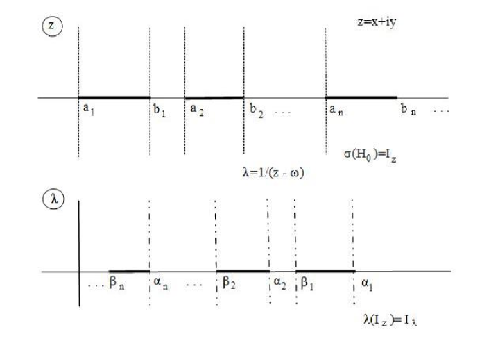
Figure 1. Sets $I=\sigma(H_{0})$ and $\lambda_{\omega}(I)$ with map $\lambda_{\omega}(z)=\frac{1}{z-\omega}$.

Lemma 2.1.

Let

(2.2) $$I=I_{z}=\bigcup^{\infty}_{k=1}[a_{k},b_{k}],\quad 0<a_{1}<b_{1}<a_{2}<b_{2}<\ldots,\quad a_{n}\to+\infty,$$

and let $\lambda_{\omega}(I)=I_{\lambda}$ be its image under the linear fractional transformation $\eqref{lft}$

$$\lambda_{\omega}(I)=I_{\lambda}=\bigcup^{\infty}_{k=1}[\beta_{k}(\omega),\alpha_{k}(\omega)],\ \ \beta_{k}(\omega)=\frac{1}{b_{k}-\omega}\,,\ \ \alpha_{k}(\omega)=\frac{1}{a_{k}-\omega}\,.$$

Then for $\omega<a_{1}$ the following bounds hold:

for $\text{\rm Re\,}z<a_{1}$ or $\text{\rm Re\,}z\in I$

(2.3) $$\frac{\operatorname{\rm d}(\lambda_{\omega}(z),\lambda_{\omega}(I)}{\operatorname{\rm d}(z,I_{z})}>\frac{1}{3|z-\omega|(|z-\omega|+a_{1}-\omega)}\,;$$

for $b_{k}<\text{\rm Re\,}z<a_{k+1}$,  $k=1,2,\ldots$

(2.4) $$\frac{\operatorname{\rm d}(\lambda_{\omega}(z),\lambda_{\omega}(I)}{\operatorname{\rm d}(z,I_{z})}\geq\frac{1}{2|z-\omega|^{2}}\,\left(1+\frac{a_{k+1}-b_{k}}{b_{k}-\omega}\right)^{-1}\,.$$

Moreover, if $\omega<0$ and the gaps are relatively bounded $\eqref{irelbound}$, then the unique bound is valid

(2.5) $$\frac{\operatorname{\rm d}(\lambda_{\omega}(z),\lambda_{\omega}(I)}{\operatorname{\rm d}(z,I_{z})}\geq\frac{1}{5(1+r(I))}\,\frac{1}{|z-\omega|(|z-\omega|+a_{1}-\omega)},\ \ z\in{\mathbb{C}}\backslash I.$$

Proof.

Let us begin with the case $\omega=0$ and put $\lambda_{0}=\lambda=z^{-1}$. If $z=x+iy$ and $x=\text{\rm Re\,}z\leq 0$, then $\text{\rm Re\,}\lambda=x|z|^{-2}\leq 0$ and so

(2.6) $$\frac{\operatorname{\rm d}(\lambda,I_{\lambda})}{\operatorname{\rm d}(z,I_{z})}=\frac{|\lambda|}{|z-a_{1}|}=\frac{1}{|z||z-a_{1}|}\geq\frac{1}{|z|(|z|+a_{1})}\,.$$

Similarly, if $x\in I_{z}$, then $x\geq a_{1}$ and

$$0<\text{\rm Re\,}\lambda=\frac{x}{|z|^{2}}\leq\frac{1}{x}\leq a_{1}^{-1}=\alpha_{1},\quad\operatorname{\rm d}(\lambda,[0,\alpha_{1}])=|\text{\rm Im\,}\lambda|=\frac{|y|}{|z|^{2}}\,.$$

Since now $\operatorname{\rm d}(z,I_{z})=|y|$, we have

(2.7) $$\frac{\operatorname{\rm d}(\lambda,I_{\lambda})}{\operatorname{\rm d}(z,I_{z})}\geq\frac{\operatorname{\rm d}(\lambda,[0,\alpha_{1}])}{\operatorname{\rm d}(z,I_{z})}=\frac{1}{|z|^{2}}>\frac{1}{|z|(|z|+a_{1})}\,.$$

Consider now the case when $x=\text{\rm Re\,}z\notin I_{z}$. Fix $x$ in $k$’s gap,

(2.8) $$b_{k}<x<a_{k+1},\qquad k=k(x)=0,1,\ldots$$

(we put $b_{0}=0$ and treat $(b_{0},a_{1})$ as a number zero gap). Then

$$\operatorname{\rm d}(z,I_{z})=\min(|z-b_{k}|,|z-a_{k+1}|),\quad k=1,2,\ldots,\quad\operatorname{\rm d}(z,I_{z})=|z-a_{1}|,\quad k=0.$$

Define two sets of positive numbers

$$u_{j}=u_{j}(x),\qquad v_{j}=v_{j}(x),\qquad j=k+1,k+2,\ldots$$

by equalities

$$\text{\rm Re\,}(\lambda(x+iu_{j}))=\frac{x}{x^{2}+u_{j}^{2}}=\alpha_{j},\qquad\text{\rm Re\,}(\lambda(x+iv_{j}))=\frac{x}{x^{2}+v_{j}^{2}}=\beta_{j},$$

or, equivalently,

$$u_{j}(x)=\sqrt{x(a_{j}-x)},\qquad v_{j}(x)=\sqrt{x(b_{j}-x)}.$$

We also put $v_{k}=0$, so

$$0=v_{k}<u_{k+1}<v_{k+1}<u_{k+2}<v_{k+2}<\ldots,\quad u_{n},\ v_{n}\to\infty,\ n\to\infty.$$

While the point $z$ traverses the line $x+iy$, $y\in{\mathbb{R}}$, its image $\lambda(z)$ describes a circle with diameter $[0,1/x]$. We discern the following two cases.

Case 1. Assume that $\lambda$ lies over the “gaps for $\lambda$”. For each $k=0,1,\ldots$ there are two options for $\lambda$: interior gaps

(2.9) $$\text{\rm Re\,}\lambda\in(\alpha_{j+1},\beta_{j})\Longleftrightarrow v_{j}<|y|<u_{j+1},\qquad j=k+1,k+2,\ldots$$

and the rightmost gap

(2.10) $$\text{\rm Re\,}\lambda\in(\alpha_{k+1},1/x)\Longleftrightarrow 0<|y|<u_{k+1}.$$

For gaps (2.9) we have

(2.11) $$\operatorname{\rm d}(\lambda,I_{\lambda})=\min(|\lambda-\alpha_{j+1}|,|\lambda-\beta_{j}|)=\frac{1}{|z|}\min\left(\frac{|z-a_{j+1}|}{a_{j+1}},\frac{|z-b_{j}|}{b_{j}}\right)\,.$$

Define an auxiliary function $h$ on the right half-line

$$h(t)=h(t,z):=\frac{|z-t|}{t}=\sqrt{\Bigl{(}\frac{x}{t}-1\Bigr{)}^{2}+y^{2}},\quad t>0.$$

Clearly, $h$ is monotone increasing on $(x,+\infty)$ and decreasing on $(0,x)$ with the minimum $h(x)=|y|$. Hence (2.11) and (2.8) give

$$\begin{split}\operatorname{\rm d}(\lambda,I_{\lambda})&=\frac{\min(h(a_{j+1},z),h(b_{j},z))}{|z|}\geq\frac{h(b_{j},z)}{|z|}\geq\frac{h(b_{k+1},z)}{|z|}\\ &\geq\frac{h(a_{k+1},z)}{|z|}=\frac{|z-a_{k+1}|}{a_{k+1}|z|}\,.\end{split}$$

Since by (2.8) $\operatorname{\rm d}(z,I_{z})\leq|z-a_{k+1}|$, we see that

(2.12) $$\frac{\operatorname{\rm d}(\lambda,I_{\lambda})}{\operatorname{\rm d}(z,I_{z})}\geq\frac{1}{a_{k+1}|z|}\,.$$

For gaps (2.10) let first $k\geq 1$. Then as above in (2.11)

$$\operatorname{\rm d}(\lambda,I_{\lambda})=\frac{1}{|z|}\min\left(\frac{|z-a_{k+1}|}{a_{k+1}},\frac{|z-b_{k}|}{b_{k}}\right)\,,$$

but it is not clear now which term prevails. If $|z-a_{k+1}|\leq|z-b_{k}|$ then $\operatorname{\rm d}(z,I_{z})=|z-a_{k+1}|$ and

$$\frac{\operatorname{\rm d}(\lambda,I_{\lambda})}{\operatorname{\rm d}(z,I_{z})}=\frac{1}{|z|}\min\left(\frac{1}{a_{k+1}},\frac{|z-b_{k}|}{b_{k}|z-a_{k+1}|}\right)=\frac{1}{a_{k+1}|z|}\,.$$

Otherwise $|z-a_{k+1}|>|z-b_{k}|$ implies

$$\frac{\operatorname{\rm d}(\lambda,I_{\lambda})}{\operatorname{\rm d}(z,I_{z})}=\frac{1}{|z|}\min\left(\frac{1}{b_{k}},\frac{|z-a_{k+1}|}{a_{k+1}|z-b_{k}|}\right)\geq\frac{1}{a_{k+1}|z|}\,.$$

Next, for $k=0$ one has $0<x<a_{1}$, and in case (2.10)

$$\operatorname{\rm d}(\lambda,I_{\lambda})=|\lambda-\alpha_{1}|=\frac{|z-a_{1}|}{a_{1}|z|}\,,\quad\operatorname{\rm d}(z,I_{z})=|z-a_{1}|,$$

and so

(2.13) $$\frac{\operatorname{\rm d}(\lambda,I_{\lambda})}{\operatorname{\rm d}(z,I_{z})}=\frac{1}{a_{1}|z|}\,.$$

Finally, in the case of “gaps for $\lambda$” we come to the bound

(2.14) $$\frac{\operatorname{\rm d}(\lambda,I_{\lambda})}{\operatorname{\rm d}(z,I_{z})}\geq\frac{1}{a_{k+1}|z|}\,,\qquad k=0,1,\ldots.$$

A modified version of (2.14) will be convenient in the sequel. For $k\geq 1$ in view of $|z|\geq x>b_{k}$ we have

$$\frac{1}{a_{k+1}|z|}\geq\frac{b_{k}}{a_{k+1}|z|^{2}}$$

and so for $k=1,2,\ldots$

(2.15) $$\frac{\operatorname{\rm d}(\lambda,I_{\lambda})}{\operatorname{\rm d}(z,I_{z})}\geq\frac{1}{|z|^{2}}\,\left(1+\frac{a_{k+1}-b_{k}}{b_{k}}\right)^{-1}=\frac{1}{|z|^{2}}\left(1+\frac{r_{k}}{b_{k}}\right)^{-1}\,,$$

$r_{k}=a_{k+1}-b_{k}$ is the length of $k$’s gap. Similarly, for $k=0$ one has from (2.13)

(2.16) $$\frac{\operatorname{\rm d}(\lambda,I_{\lambda})}{\operatorname{\rm d}(z,I_{z})}\geq\frac{1}{|z|(|z|+a_{1})}\,.$$

Case 2. Assume that $\lambda$ lies over the “bands for $\lambda$”

(2.17) $$\text{\rm Re\,}\lambda\in[\beta_{j},\alpha_{j}]\Longleftrightarrow u_{j}\leq|y|\leq v_{j},\qquad j=k+1,k+2,\ldots.$$

Now

$$\operatorname{\rm d}(\lambda,I_{\lambda})=|\text{\rm Im\,}\lambda|=\frac{|y|}{|z|^{2}}\,,$$

$$\begin{split}\operatorname{\rm d}(z,I_{z})&\leq|z-a_{k+1}|\leq|y|+a_{k+1}-x=|y|+\frac{u_{k+1}^{2}}{x}\leq|y|\left(1+\frac{u_{k+1}}{x}\right)\\ &=|y|\left(1+\sqrt{\frac{a_{k+1}-x}{x}}\right),\end{split}$$

so that

(2.18) $$\frac{\operatorname{\rm d}(\lambda,I_{\lambda})}{\operatorname{\rm d}(z,I_{z})}\geq\frac{1}{|z|^{2}}\,\left(1+\sqrt{\frac{a_{k+1}}{x}-1}\right)^{-1}\,.$$

For $k\geq 1$ (interior gap for $z$) inequality (2.18) can be simplified in view of $x>b_{k}$

(2.19) $$\frac{\operatorname{\rm d}(\lambda,I_{\lambda})}{\operatorname{\rm d}(z,I_{z})}\geq\frac{1}{|z|^{2}}\,\left(1+\sqrt{\frac{r_{k}}{b_{k}}}\right)^{-1}\,.$$

Let now $k=0$, i.e., $0<x=\text{\rm Re\,}z<a_{1}$. In our case $\operatorname{\rm d}(z,I_{z})=|z-a_{1}|$ and

$$|y|\geq u_{1}=\sqrt{x(a_{1}-x)}.$$

If $|y|\geq 2x$ then $|y|\geq\frac{2}{3}|z|$ and so

(2.20) $$\frac{\operatorname{\rm d}(\lambda,I_{\lambda})}{\operatorname{\rm d}(z,I_{z})}=\frac{|y|}{|z|^{2}|z-a_{1}|}\geq\frac{2}{3}\frac{1}{|z|(|z|+a_{1})}\,.$$

Otherwise, $|y|<2x$ implies

$$2\sqrt{x}>\sqrt{a_{1}-x},\qquad x>\frac{a_{1}}{5}.$$

It follows now from (2.18) with $k=0$ that

(2.21) $$\frac{\operatorname{\rm d}(\lambda,I_{\lambda})}{\operatorname{\rm d}(z,I_{z})}\geq\frac{1}{3|z|^{2}}>\frac{1}{3}\frac{1}{|z|(|z|+a_{1})}\,.$$

We can summarize the results obtained above in the following two bounds from below. A combination of (2.6), (2.7), (2.16) and (2.21) gives

(2.22) $$\frac{\operatorname{\rm d}(\lambda,I_{\lambda})}{\operatorname{\rm d}(z,I_{z})}>\frac{1}{3|z|(|z|+a_{1})}\,,\qquad\text{\rm Re\,}z<a_{1}\ \ {\rm or}\ \text{\rm Re\,}z\in I_{z}.$$

A combination of (2.15) and (2.19) provides

(2.23) $$\begin{split}\frac{\operatorname{\rm d}(\lambda,I_{\lambda})}{\operatorname{\rm d}(z,I_{z})}&\geq\frac{1}{\gamma_{k}|z|^{2}}\,,\qquad\gamma_{k}=\max\left\{1+\frac{r_{k}}{b_{k}},\ 1+\sqrt{\frac{r_{k}}{b_{k}}}\right\}\,,\\ b_{k}&<\text{\rm Re\,}z<a_{k+1},\quad k=1,2,\ldots.\end{split}$$

Since $\gamma_{k}<2(1+r_{k}/b_{k})$, the latter can be written as

(2.24) $$\frac{\operatorname{\rm d}(\lambda,I_{\lambda})}{\operatorname{\rm d}(z,I_{z})}\geq\frac{1}{2|z|^{2}}\,\left(1+\frac{r_{k}}{b_{k}}\right)^{-1}\,,\quad b_{k}<\text{\rm Re\,}z<a_{k+1},\quad k=1,2,\ldots.$$

To work out the general case $\omega\not=0$ and prove (2.3) and (2.4), it remains only to shift the variable and apply the results just obtained to the shifted sequence of bands

$$I_{z}(\omega)=\bigcup_{k\geq 1}[a_{k}-\omega,b_{k}-\omega].$$

The final statement follows from a simple observation

$$\frac{r_{k}}{b_{k}-\omega}\leq\frac{r_{k}}{b_{k}}\leq r.$$

The proof is complete. ∎

3. Lieb–Thirring type inequalities

We continue with Hansmann’s inequality (1.1) and the upper (lower) bounds for its right (left) hand sides obtained in previous sections. In what follows, $C_{k}=C_{k}(p,d,I)$, $k=1,2,\ldots$, denote positive constants, which depend on $p,d$, and the set $I$ (0.2).

Proposition 3.1.

Under conditions of Theorem 0.1, for $\omega\leq\omega_{0}$ defined in $\eqref{omega}$, we have

(3.1) $$\sum_{z\in\sigma_{d}(H)}\frac{\operatorname{\rm d}^{p}(z,I)}{|z-\omega|^{p}(|z-\omega|+a_{1}-\omega)^{p}}\leq C_{1}\,\frac{\|V\|^{p}_{p}}{|\omega|^{(q+1)p}},\quad\omega\leq\omega_{0}.$$

Proof.

We apply (1.1) with

$$A_{0}=A_{0}(\omega)=R(\omega,H_{0}),\qquad A=A(\omega)=R(\omega,H).$$

So, by Lemma 1.1, with $I_{\lambda}=\lambda_{\omega}(I)=\sigma(A_{0})$

(3.2) $$\begin{split}&\sum_{\lambda\in\sigma_{d}(A)}\operatorname{\rm d}^{p}(\lambda,I_{\lambda})=\sum_{\lambda\in\sigma_{d}(A)}\operatorname{\rm d}^{p}(\lambda,\sigma(A_{0}))\\ &\leq K\,\|R(\omega,H)-R(\omega,H_{0})\|^{p}_{\mathcal{S}_{p}}\leq C_{2}\,\frac{\|V\|^{p}_{p}}{|\omega|^{(q+1)p}}\,.\end{split}$$

Lemma 2.1 completes the proof of (3.1) as

$$\sum_{z\in\sigma_{d}(H)}\frac{\operatorname{\rm d}^{p}(z,I)}{|z-\omega|^{p}(|z-\omega|+a_{1}-\omega)^{p}}\leq C_{3}(1+r(I))^{p}\,\frac{\|V\|^{p}_{p}}{|\omega|^{(q+1)p}}=C_{4}\,\frac{\|V\|^{p}_{p}}{|\omega|^{(q+1)p}}.$$

∎

Proof of Theorem 0.1. The idea of the proof is to use the above proposition and a “convergence improving trick” from [5, p. 2754].

Put $\alpha:=p(q+1)-1-\tau>0$, and rewrite inequality (3.1) in the form

$$\sum_{z\in\sigma_{d}(H)}\frac{\operatorname{\rm d}^{p}(z,I)\cdot s^{\alpha}}{|z+s|^{p}(|z+s|+a_{1}+s)^{p}}\leq C_{1}\,\frac{\|V\|^{p}_{p}}{s^{1+\tau}},$$

where $s:=|\omega|\geq s_{0}:=|\omega_{0}|$. Observe that

$$|z+s|\leq|z|+s,\quad|z+s|+a_{1}+s\leq 2s+|z|+a_{1},$$

and so

$$\sum_{z\in\sigma_{d}(H)}\frac{\operatorname{\rm d}^{p}(z,I)\cdot s^{\alpha}}{(s+|z|)^{p}(2s+|z|+a_{1})^{p}}\leq C_{1}\,\frac{\|V\|^{p}_{p}}{s^{1+\tau}}\,.$$

Next, integrate the latter inequality with respect to $s$ from $s_{0}$ to infinity and change the order of summation and integration

$$\sum_{z\in\sigma_{d}(H)}\operatorname{\rm d}^{p}(z,I)\,\int^{\infty}_{s_{0}}\frac{s^{\alpha}\,ds}{(s+|z|)^{p}(2s+|z|+a_{1})^{p}}\leq C_{1}\,\frac{\|V\|^{p}_{p}}{\tau s_{0}^{\tau}}.$$

The integral in the left-hand side converges, since

$$\alpha>0,\qquad 2p-\alpha-1=d/2+\tau>0.$$

Making the change of variables $s=(|z|+s_{0})t+s_{0}$ and noticing that

$$2s+|z|+a_{1}=2(|z|+s_{0})t+2s_{0}+|z|+a_{1}\leq 3(|z|+s_{0})(t+1)$$

(see (0.8)), we come to

$$\begin{split}\int^{\infty}_{s_{0}}\frac{s^{\alpha}\,ds}{(s+|z|)^{p}(2s+|z|+a_{1})^{p}}&\geq\frac{1}{3^{p}(|z|+s_{0})^{2p-\alpha-1}}\,\int_{0}^{\infty}\frac{t^{\alpha}\,dt}{(1+t)^{2p}}\\ &=\frac{C(p,d,\tau)}{(|z|+s_{0})^{d/2+\tau}}\,,\end{split}$$

which gives (0.9). The proof of the theorem is complete. $\Box$

Proof of Corollary 0.2. Certainly, $|z|+s_{0}\leq(1+s_{0})(1+|z|)$, and $(1+s_{0})/s_{0}\leq 2$. Hence

(3.3) $$\begin{split}\sum_{z\in\sigma_{d}(H)}\frac{\operatorname{\rm d}^{p}(z,J)}{(1+|z|)^{d/2+\tau}}&\leq C_{2}(1+s_{0})^{d/2}\left(\frac{1+\omega_{0}}{\omega_{0}}\right)^{\tau}\|V\|^{p}_{p}\\ &\leq C(p,d,I,\tau)(1+|\omega_{0}|)^{d/2}\,\|V\|^{p}_{p},\end{split}$$

as claimed. Furthermore, by (0.8)

$$1+s_{0}\leq C_{3}(1+\|V_{0}\|_{\infty})(1+\|V\|^{1/q}_{p})\leq C_{3}(1+\|V_{0}\|_{\infty})(1+\|V\|_{p})^{1/q},$$

and inequality (3.3) reads

$$\sum_{z\in\sigma_{d}(H)}\frac{\operatorname{\rm d}^{p}(z,I)}{(1+|z|)^{d/2+\tau}}\leq C(p,d,I,\tau)\,(1+\|V_{0}\|_{\infty})^{d/2}(1+\|V\|_{p})^{d/2q}\,\|V\|^{p}_{p}.$$

It remains to note that $d/2<d/2q$, so (1.5) follows. The proof of corollary is complete. $\Box$

Let us mention that inequality (1.5) is better (regarding the powers) than the corresponding result in [13, Theorem 0.2].

Acknowledgments. The authors are grateful to F. Gesztesy for a detailed account on the Kato method. They also thank M. Hansmann for valuable discussions on the subject of the article. The paper was prepared during the visit of the first author to the Institute of Mathematics of Bordeaux (IMB UMR5251) at University of Bordeaux. He would like to thank this institution for the hospitality and acknowledges the financial support of “IdEx of University of Bordeaux”.

References

- [1] A. Borichev, L. Golinskii, S. Kupin, A Blaschke-type condition and its application to complex Jacobi matrices, Bull. Lond. Math. Soc. 41 (2009), no. 1, 117-123.
- [2] A. Borichev, L. Golinskii, S. Kupin, New Blaschke-type conditions on zeros of analytic functions from certain classes, preprint, 2015.
- [3] J.C. Cuenin, Eigenvalue bounds for Dirac and fractional Schrödinger operators with complex potentials, submitted; see also http://arxiv.org/abs/1506.07193.
- [4] E. B. Davies, Linear Operators and their Spectra, Cambridge University Press, Cambridge, 2007.
- [5] M. Demuth, M. Hansmann, G. Katriel, On the discrete spectrum of non-selfadjoint operators, J. Funct. Anal. 257 (2009), 2742-2759.
- [6] C. Dubuisson, On quantitative bounds on eigenvalues of a complex perturbation of a Dirac operator, Int. Eq. Oper. Theory 78 (2014), no. 2, 249-269.
- [7] C. Dubuisson, Notes on Lieb-Thirring type inequality for a complex perturbation of fractional Schrödinger operator, to appear in Zh. Mat. Fiz. Anal. Geom.; see also http://arxiv.org/abs/1403.5116.
- [8] C. Dubuisson, L. Golinskii, S. Kupin, New versions of Lieb–Thirring inequalities for complex perturbations of certain model operators, preprint, 2015.
- [9] R. Frank, A. Laptev, E. Lieb, R. Seiringer, Lieb-Thirring inequalities for Schrödinger operators with complex-valued potentials, Lett. Math. Phys. 77 (2006), no. 3, 309-316.
- [10] R. Frank, J. Sabin, Restriction theorems for orthonormal functions, Strichartz inequalities, and uniform Sobolev estimates, submitted; see also http://arxiv.org/abs/1404.2817.
- [11] R. Frank, B. Simon, Eigenvalue bounds for Schrödinger operators with complex potentials, II, submitted; see also http://arxiv.org/abs/1504.01144.
- [12] F. Gesztesy, Y. Latushkin, M. Mitrea, M. Zinchenko, Nonselfadjoint operators, infinite determinants, and some applications, (English summary) Russ. J. Math. Phys. 12 (2005), no. 4, 443-471; see also http://arxiv.org/abs/math/0511371.
- [13] L. Golinskii, S. Kupin, On discrete spectrum of complex perturbations of finite band Schrödinger operators, in : ”Recent trends in analysis : proceedings of the conference in honor of Nikolai Nikolski: Bordeaux, 2011”, Theta Foundation, Bucarest, 2013.
- [14] L. Golinskii, S. Kupin, On complex perturbations of infinite band Schrödinger operators, to appear in Methods Funct. Anal. Topology; see also http://arxiv.org/abs/1502.06022.
- [15] M. Hansmann, On the discrete spectrum of linear operators in Hilbert spaces, Ph.D. thesis, TU Clausthal, 2010.
- [16] M. Hansmann, Variation of discrete spectra for non-selfadjoint perturbations of selfadjoint operators, Int. Eq. Op. Theory 76(1) (2013) 163-178.
- [17] M. Hansmann, An eigenvalue estimate and its application to non-self-adjoint Jacobi and Schrödinger operators, Lett. Math. Phys. 98 (2011), 79-95.
- [18] T. Kato, Wave operators and similarity for some non-selfadjoint operators, Math. Ann. 162 (1965-1966), 258-279.
- [19] A. Laptev and O. Safronov, Eigenvalues estimates for Schrödinger operators with complex potentials, Commun. Math. Phys. bf 292 (1) (2009), 29-54.
- [20] V. Marchenko, I. Ostrovskii, A characterization of the spectrum of the Hill operator, Math. USSR Sbornik 26 (1975), 493-554.
- [21] M. Reed, B. Simon, Methods of modern mathematical physics, vol. 4, Analysis of Operators. Academic Press, Inc., New York, 1978.
- [22] D. Sambou, Lieb-Thirring type inequalities for non-self-adjoint perturbations of magnetic Schrödinger operators, J. Funct. Anal. 266 (2014), no. 8, 5016-5044.
- [23] B. Simon, Trace ideals and their applications, Mathematical Surveys and Monographs, vol. 120. AMS, Providence, RI, 2005.