Notes on a PDE System

for Biological Network Formation

Jan Haskovec  Peter Markowich  Benoît Perthame  Matthias Schlottbom

Abstract. We present new analytical and numerical results for the elliptic-parabolic system of partial differential equations proposed by Hu and Cai [8, 10], which models the formation of biological transport networks. The model describes the pressure field using a Darcy’s type equation and the dynamics of the conductance network under pressure force effects. Randomness in the material structure is represented by a linear diffusion term and conductance relaxation by an algebraic decay term. The analytical part extends the results of [7] regarding the existence of weak and mild solutions to the whole range of meaningful relaxation exponents. Moreover, we prove finite time extinction or break-down of solutions in the spatially one-dimensional setting for certain ranges of the relaxation exponent. We also construct stationary solutions for the case of vanishing diffusion and critical value of the relaxation exponent, using a variational formulation and a penalty method.

The analytical part is complemented by extensive numerical simulations. We propose a discretization based on mixed finite elements and study the qualitative properties of network structures for various parameters values. Furthermore, we indicate numerically that some analytical results proved for the spatially one-dimensional setting are likely to be valid also in several space dimensions.

Key words: Network formation; Weak solutions; Stability; Penalty method; Numerical experiments.

Math. Class. No.: 35K55; 35B32; 92C42

1 Introduction

In [7] we presented a mathematical analysis of the PDE system modeling formation of biological transportation networks

$$-\nabla\cdot[(rI+m\otimes m)\nabla p] = S,$$ (1.1)

$$\frac{\partial m}{\partial t}-D^{2}\Delta m-c^{2}(m\cdot\nabla p)\nabla p+\alpha|m|^{2(\gamma-1)}m = 0,$$ (1.2)

for the scalar pressure $p=p(t,x)\in\mathbb{R}$ of the fluid transported within the network and vector-valued conductance $m=m(t,x)\in\mathbb{R}^{d}$ with $d\leq 3$ the space dimension. The parameters are $D\geq 0$ (diffusivity), $c>0$ (activation parameter), $\alpha>0$ and $\gamma\in\mathbb{R}$; in particular, we restricted ourselves to $\gamma\geq 1$ in [7]. The scalar function $r=r(x)\geq r_{0}>0$ describes the isotropic background permeability of the medium. The source term $S=S(x)$ is assumed to be independent of time and $\gamma\in\mathbb{R}$ is a parameter crucial for the type of networks formed [10]. In particular, experimental studies of scaling relations of conductances (diameters) of parent and daughter edges in realistic network modeling examples suggest that $\gamma=1/2$ can be used to model blood vessel systems in the human body and $\gamma=1$ is adapted to leaf venation [8, 9]. For the details on the modeling which leads to (1.1), (1.2) we refer to [1].

The system was originally derived in [8, 10] as the formal gradient flow of the continuous version of an energy functional describing formation of biological transportation networks on discrete graphs. We pose (1.1), (1.2) on a bounded domain $\Omega\subset\mathbb{R}^{d}$ with smooth boundary $\partial\Omega$, subject to homogeneous Dirichlet boundary conditions on $\partial\Omega$ for $m$ and $p$:

$$m(t,x)=0,\qquad p(t,x)=0\qquad\mbox{for }x\in\partial\Omega,\;t\geq 0,$$ (1.3)

and subject to the initial condition for $m$:

$$m(t=0,x)=m^{0}(x)\qquad\mbox{for }x\in\Omega.$$ (1.4)

The main mathematical interest of the PDE system for network formation stems from the highly unusual nonlocal coupling of the elliptic equation (1.1) for the pressure $p$ to the reaction-diffusion equation (1.2) for the conductance vector $m$ via the pumping term $+c^{2}(\nabla p\otimes\nabla p)m$ and the latter term’s potential equilibriation with the decay term $-|m|^{2(\gamma-1)}m$. A major observation concerning system (1.1)–(1.2) is that it represents the formal $L^{2}(\Omega)$-gradient flow associated with the highly non-convex energy-type functional

$$\mathcal{E}(m):=\frac{1}{2}\int_{\Omega}\left(D^{2}|\nabla m|^{2}+\frac{\alpha}{\gamma}|m|^{2\gamma}+c^{2}|m\cdot\nabla p[m]|^{2}+c^{2}r(x)|\nabla p[m]|^{2}\right)\,\mathrm{d}x,$$ (1.5)

where $p=p[m]\in H^{1}_{0}(\Omega)$ is the unique solution of the Poisson equation (1.1) with given $m$, subject to the homogeneous Dirichlet boundary condition on $\partial\Omega$. Note that (1.5) consists of, respectively, the diffusive energy term, metabolic (relaxation) energy, and the last two terms account for network-fluid interaction energy. We have:

Lemma 1 (Lemma 1 in [7]).

Let $\mathcal{E}(m^{0})<\infty$. Then the energy $\mathcal{E}(m(t))$ is nonincreasing along smooth solutions of (1.1)–(1.2) and satisfies

$$\frac{\,\mathrm{d}}{\,\mathrm{d}t}\mathcal{E}(m(t))=-\int_{\Omega}\left(\frac{\partial m}{\partial t}(t,x)\right)^{2}\,\mathrm{d}x.$$

As usual, along weak solutions, we obtain a weaker form of energy dissipation, see formula (2.4) below.

In [7] we provided the following analytical results for (1.1)–(1.4) in the case $\gamma\geq 1$:

• Existence of global weak solutions in the energy space

• Existence and uniqueness of local in time mild solutions (global in 1d)

• Existence of nontrivial (i.e., $m\not\equiv 0$) stationary states and analysis of their stability (nonlinear in 1d, linearized in multiple dimensions)

• The limit $D\to 0$ in the 1d setting

The purpose of this paper is to extend the analysis of the network formation system by providing several new results, in particular:

• Existence of global weak solutions in the energy space for $1/2\leq\gamma<1$ and of local in time mild solutions for $1/2<\gamma<1$ (Section 2).

• Analysis of the system in the 1d setting: finite time breakdown of solutions for $\gamma<1/2$, infinite time extinction for $1/2\leq\gamma\leq 1$ with small sources, nonlinear stability analysis for $\gamma\geq 1/2$ and $D=0$ (Section 3).

• Construction of stationary solutions in the case $\gamma=1$ and $D=0$ (Section 4).

The analytical part is complemented by extensive numerical examples in Section 5. We propose a discretization based on mixed finite elements and study the qualitative properties of network structures for various parameters values. Furthermore, we indicate numerically that some analytical results proved for the spatially one-dimensional setting are likely to be valid also in several space dimensions.

1.1 Scaling analysis

We introduce the rescaled variables

$$x_{s}:=\frac{x}{\overline{x}},\qquad t_{s}:=\frac{t}{\overline{t}},\qquad m_{s}:=\frac{m}{\overline{m}},\qquad p_{s}:=\frac{p}{\overline{p}},\qquad S_{s}:=\frac{S}{\overline{S}}$$

and choose

$$\overline{x}:=\mbox{diam}(\Omega),\qquad\overline{m}:=\sup_{x\in\Omega}|m^{0}(x)|,\qquad\overline{t}:=\frac{1}{\alpha\overline{m}^{2(\gamma-1)}},\qquad\overline{S}:=\sup_{x\in\Omega}|S(x)|,\qquad\overline{p}:=\frac{\overline{x}^{2}\overline{S}}{\overline{m}^{2}}$$

which leads to $S_{s}=\mathcal{O}(1)$, $m_{s}(t=0)=\mathcal{O}(1)$ and the following rescaled version of (1.1)–(1.2),

$$-\nabla_{x_{s}}\cdot[(r_{s}I+m\otimes m)\nabla_{x_{s}}p_{s}] = S_{s},$$

$$\frac{\partial m_{s}}{\partial t}-D_{s}^{2}\Delta_{x_{s}}m_{s}-c_{s}^{2}(m_{s}\cdot\nabla_{x_{s}}p_{s})\nabla p_{s}+|m_{s}|^{2(\gamma-1)}m_{s} = 0,$$

with

$$r_{s}=\frac{r}{\overline{m}^{2}},\qquad D_{s}^{2}=\frac{\overline{p}\,\overline{m}^{2}}{\overline{x}^{2}\overline{s}},\qquad c_{s}^{2}=\frac{c^{2}\overline{p}^{2}}{\alpha\overline{x}^{2}\overline{m}^{2(\gamma-1)}}.$$

Dropping the index $s$ in the scaled variables, we obtain the system

$$-\nabla\cdot[(rI+m\otimes m)\nabla p] = S,$$ (1.6)

$$\frac{\partial m}{\partial t}-D^{2}\Delta m-c^{2}(m\cdot\nabla p)\nabla p+|m|^{2(\gamma-1)}m = 0,$$ (1.7)

that we will study in this paper. Moreover, for simplicity, we set $r(x)\equiv 1$ in the analytical part (Sections 2–4).

Convention.

In the following, generic, not necessarily equal, constants will be denoted by $C$. Moreover, we will make specific use of the Poincaré constant $C_{\Omega}$, i.e.,

$$\left\|u\right\|_{L^{2}(\Omega)}\leq C_{\Omega}\left\|\nabla u\right\|_{L^{2}(\Omega)}\qquad\mbox{for all }u\in H_{0}^{1}(\Omega).$$

2 Existence of global weak solutions for $1/2\leq\gamma<1$

In [7], Section 2, we provided the proof of existence of global weak solutions for $\gamma\geq 1$ based on the Leray-Schauder fixed point theorem for a regularized version of (1.6)–(1.7) that preserves the energy dissipation structure, and consequent limit passage to remove the regularization. We now extend the proof to the case $1/2\leq\gamma<1$. However, the case $\gamma=1/2$ requires special care since the algebraic term in (1.7) formally becomes $m/|m|$ and an interpretation has to be given for $m=0$. In particular, (1.7) has to be substituted by the differential inclusion

$$\partial_{t}m-D^{2}\Delta m-c^{2}(m\cdot\nabla p[m])\nabla p[m]\in-\partial\mathcal{R}(m),$$ (2.1)

where $\partial\mathcal{R}$ is the subdifferential of $\mathcal{R}(m):=\int_{\Omega}|m|\,\mathrm{d}x$, in particular,

$$\partial\mathcal{R}(m)=\{u\in L^{\infty}(\Omega)^{d};\,u(x) = m(x)/|m(x)|\mbox{ if }m(x)\neq 0,$$ (2.2)

$$|u(x)| \leq 1\mbox{ if }m(x)=0\}.$$ (2.3)

Theorem 1 (Extension of Theorem 1 of [7]).

Let $\gamma\geq 1/2$, $S\in L^{2}(\Omega)$ and $m^{0}\in H_{0}^{1}(\Omega)^{d}\cap L^{2\gamma}(\Omega)^{d}$. Then the problem (1.6)–(1.7), (1.3)–(1.4) (with (2.1) instead of (1.7) if $\gamma=1/2$) admits a global weak solution $(m,p[m])$ with $\mathcal{E}(m)\in L^{\infty}(0,\infty)$ and with

$$m\in L^{\infty}(0,\infty;H_{0}^{1}(\Omega))\cap L^{\infty}(0,\infty;L^{2\gamma}(\Omega)), \partial_{t}m\in L^{2}((0,\infty)\times\Omega),$$

$$\nabla p\in L^{\infty}(0,\infty;L^{2}(\Omega)), m\cdot\nabla p\in L^{\infty}(0,\infty;L^{2}(\Omega)).$$

This solution satisfies the energy dissipation inequality, with $\mathcal{E}$ given by (1.5),

$$\mathcal{E}(m(t))+\int_{0}^{t}\int_{\Omega}\left(\frac{\partial m}{\partial t}(s,x)\right)^{2}\,\mathrm{d}x\,\mathrm{d}s\leq\mathcal{E}(m^{0})\qquad\mbox{for all }t\geq 0.$$ (2.4)

The proof proceeds along the lines of Section 2 of [7], i.e., for $\gamma>1/2$ and $\varepsilon>0$ we consider the regularized system

$$-\nabla\cdot[\nabla p+m(m\cdot\nabla p)\ast\eta_{\varepsilon}] = S,$$ (2.5)

$$\frac{\partial m}{\partial t}-D^{2}\Delta m-c^{2}[(m\cdot\nabla p)\ast\eta_{\varepsilon}]\nabla p+|m|^{2(\gamma-1)}m = 0,$$ (2.6)

with $(\eta_{\varepsilon})_{\varepsilon>0}$ the $d$-dimensional heat kernel $\eta_{\varepsilon}(x)=(4\pi\varepsilon)^{-d/2}\exp(-|x|^{2}/4\varepsilon)$ and $m$, $p$ are extended by $0$ outside $\Omega$ so that the convolution is well defined. For $\gamma=1/2$, equation (2.6) has to be substituted by the differential inclusion

$$\frac{\partial m}{\partial t}-D^{2}\Delta m-c^{2}[(m\cdot\nabla p)\ast\eta_{\varepsilon}]\nabla p\in-\partial\mathcal{R}(m).$$

Weak solutions of the regularized system are constructed by an application of the Leray-Schauder fixed point theorem as in Section 2 in [7], the only change that needs to be done is a slight modification of the proof of Lemma 3 in [7]. In particular, for $\gamma>1/2$ we construct weak solutions of the auxiliary problem

$$\frac{\partial m}{\partial t}-D^{2}\Delta m-f=-|m|^{2(\gamma-1)}m,$$ (2.7)

subject to the initial and boundary conditions

$$m(t=0)=m^{0}\quad\mbox{in }\Omega,\qquad m=0\quad\mbox{on }\partial\Omega.$$ (2.8)

Again, for $\gamma=1/2$ we have to consider the following differential inclusion instead,

$$\frac{\partial m}{\partial t}-D^{2}\Delta m-f\in-\partial\mathcal{R}(m).$$ (2.9)

In the subsequent lemma we construct the so-called slow solution of (2.9), which is the unique weak solution of the PDE

$$\frac{\partial m}{\partial t}-D^{2}\Delta m-f=-r(m)$$ (2.10)

with

$$[r(m)](x)=\left\{\begin{array}[]{ll}m(x)/|m(x)|&\mbox{ when }m(x)\neq 0,\\ 0&\mbox{ when }m(x)=0.\end{array}\right.$$ (2.11)

Lemma 2 (Extension of Lemma 3 in [7]).

For every $D>0$, $\gamma>1/2$, $T>0$ and $f\in L^{2}((0,T)\times\Omega)^{d}$, the problem (2.7)–(2.8) with $m^{0}\in H_{0}^{1}(\Omega)^{d}$ admits a unique weak solution $m\in L^{\infty}(0,T;H_{0}^{1}(\Omega))^{d}\cap L^{2}(0,T;H^{2}(\Omega))^{d}\cap L^{\infty}(0,T;L^{2\gamma}(\Omega))^{d}$ with $\partial_{t}m\in L^{2}((0,T)\times\Omega)^{d}$ and the estimates hold

$$\left\|m\right\|_{L^{\infty}(0,T;H_{0}^{1}(\Omega))} \leq C\left(\left\|f\right\|_{L^{2}((0,T)\times\Omega)}+\left\|m^{0}\right\|_{H_{0}^{1}(\Omega)}\right),$$ (2.12)

$$\left\|\Delta m\right\|_{L^{2}((0,T)\times\Omega)} \leq C\left(\left\|f\right\|_{L^{2}((0,T)\times\Omega)}+\left\|m^{0}\right\|_{H^{1}_{0}(\Omega)}\right).$$ (2.13)

The same statement is true for the problem (2.10)–(2.11), (2.8) in the case $\gamma=1/2$.

Proof.

In both cases (i.e. $\gamma\geq 1/2$) we construct the solution of the differential inclusion

$$\frac{\partial m}{\partial t}+\partial\mathcal{I}_{\gamma}(m)\ni f$$ (2.14)

with the functional $\mathcal{I}_{\gamma}:L^{2}(\Omega)\to[0,+\infty]$ given by

$$\mathcal{I}_{\gamma}(m):=\frac{D^{2}}{2}\int_{\Omega}|\nabla m|^{2}\,\mathrm{d}x+\frac{1}{2\gamma}\int_{\Omega}|m|^{2\gamma}\,\mathrm{d}x,\qquad\mbox{if }m\in H^{1}_{0}(\Omega)\cap L^{2\gamma}(\Omega),$$

and $\mathcal{I}_{\gamma}(m):=+\infty$ otherwise. It can be easily checked that for $\gamma\geq 1/2$ the functional $\mathcal{I}_{\gamma}$ is proper with dense domain, strictly convex and lower semicontinuous on $H^{1}_{0}(\Omega)$. By the Rockafellar theorem [13], the Fréchet subdifferential $\partial\mathcal{I}_{\gamma}(m)$ is a maximal monotone operator and the standard theory [2] then provides the existence of a unique solution $m\in L^{2}(0,T;H^{1}_{0}(\Omega))^{d}\cap L^{2\gamma}((0,T)\times\Omega)^{d}$ of (2.14). Clearly, for $\gamma>1/2$, $m$ is the unique weak solution of (2.7)–(2.8). For $\gamma=1/2$, $m$ is the so-called slow solution, meaning that the velocity $\frac{\,\mathrm{d}m}{\,\mathrm{d}t}$ is the element of minimal norm in $\partial\mathcal{R}(m)$, i.e.,

$$\frac{\,\mathrm{d}m}{\,\mathrm{d}t}=-\mbox{argmin}\{\left\|u\right\|_{H^{1}_{0}(\Omega)};u\in\partial\mathcal{R}(m)\}.$$

Therefore, $m$ is a weak solution of (2.10)–(2.11).

To prove the higher regularity estimates (2.12), (2.13), we use (formally, but easily justifiable) $\Delta m$ as a test function, which after integration by parts leads to

$$\frac{1}{2}\frac{\,\mathrm{d}}{\,\mathrm{d}t}\int_{\Omega}|\nabla m|^{2}\,\mathrm{d}x+D^{2}\int_{\Omega}|\Delta m|^{2}\,\mathrm{d}x-\int_{\Omega}(|m|^{2(\gamma-1)}m)\cdot\Delta m\,\mathrm{d}x=\int_{\Omega}f\cdot\Delta m\,\mathrm{d}x.$$ (2.15)

Then, denoting $\varphi(m):=|m|^{2(\gamma-1)}m$, we have

$$-\int_{\Omega}(|m|^{2(\gamma-1)}m)\cdot\Delta m\,\mathrm{d}x=-\int_{\Omega}\varphi(m)\cdot\Delta m\,\mathrm{d}x=\int_{\Omega}\nabla m\cdot D\varphi(m)\nabla m\,\mathrm{d}x$$ (2.16)

with

$$D\varphi(m)=|m|^{2(\gamma-1)}\left(2(\gamma-1)\frac{m}{|m|}\otimes\frac{m}{|m|}+I\right).$$

Clearly, $D\varphi(m)$ is a nonnegative matrix for $\gamma\geq 1/2$, so that the term (2.16) is nonnegative. The identity (2.15) together with a standard density argument gives directly the required regularity and the estimates (2.12), (2.13).

 

The rest of the proof of existence of solutions of the regularized problem (2.5)–(2.6) is identical to Section 2 of [7]. For the limit $\varepsilon\to 0$, we only need to provide the following result for the case $\gamma=1/2$.

Lemma 3.

Let $m^{k}\to m$ strongly in $L^{1}((0,T)\times\Omega)$ as $k\to\infty$, and denote $h^{k}:=r(m^{k})$ with $r$ given by (2.11). Then there exists $h\in\partial\mathcal{R}(m)$ such that, for a whileuence,

$$h^{k}\rightharpoonup^{*}h\qquad\mbox{weakly* in }L^{\infty}((0,T)\times\Omega)\mbox{ as }k\to\infty.$$

Proof: Because $h^{k}=r(m^{k})$ is uniformly bounded in $L^{\infty}((0,T)\times\Omega)$, there exists a subsequence, still denoted by $h^{k}$, converging to $h\in L^{\infty}((0,T)\times\Omega)$ weakly*. Due to the strong convergence of $m^{k}$ in $L^{1}$, there exists a subsequence converging almost everywhere to $m$. Consequently, $h^{k}$ converges to $m/|m|$ almost everywhere on $\{m\neq 0\}$. On $\{m=0\}$, we have $|h|\leq 1$, so that $h\in\partial\mathcal{R}(m)$ defined by (2.2).

 

Note that in the case $\gamma=1/2$, due to Lemma 3, we only obtain weak solutions of the system (1.6), (2.1). We conjecture that $m$ is in fact a slow solution of (2.1), i.e., that it solves

$$\partial_{t}m-D^{2}\Delta m-c^{2}(m\cdot\nabla p[m])\nabla p[m]=r(m)$$

with $r(m)$ given by (2.11).

Remark 1.

The proof of local in time existence of mild solutions (Theorem 3 of [7]) carries over to the case $1/2<\gamma<1$ without modifications. However, the proof of uniqueness of mild solutions by a contraction mapping argument requires $\gamma\geq 1$ and it is not clear how to adapt it for values of $\gamma$ less than one.

3 Analysis in the 1d setting

Much more can be proved about the system (1.6)–(1.7) in the spatially one dimensional setting. Then, and without loss of generality, we can consider it on the interval $\Omega:=(0,1)$. The system reads

$$-\partial_{x}\bigl{(}\partial_{x}p+m^{2}\partial_{x}p\bigr{)} = S,$$ (3.1)

$$\partial_{t}m-D^{2}\partial_{xx}^{2}m-c^{2}(\partial_{x}p)^{2}m+|m|^{2(\gamma-1)}m = 0,$$ (3.2)

Additionally, throughout this section we assume $S>0$ a.e. on $(0,1$), and for mathematical convenience we prescribe the mixed boundary conditions for $p$,

$$\partial_{x}p(0)=0,\qquad p(1)=0,$$

and homogeneous Neumann boundary condition for $m$. Then, integrating (3.1) with respect to $x$, we obtain

$$(1+m^{2})\partial_{x}p=-\int_{0}^{x}S(y)\,\mathrm{d}y.$$

Denoting $B(x):=\int_{0}^{x}S(y)\,\mathrm{d}y$, we have

$$\partial_{x}p=-\frac{B(x)}{1+m^{2}},$$ (3.3)

so that the system (3.1)–(3.2) is rewritten as

$$\partial_{t}m-D^{2}\partial_{xx}^{2}m=\left(\frac{c^{2}B(x)^{2}}{(1+m^{2})^{2}}-|m|^{2(\gamma-1)}\right)m.$$ (3.4)

3.1 Extinction of solutions for $-1\leq\gamma\leq 1$ and small sources

We show that if the source term $S$ is small enough in a suitable sense, then solutions of (3.4) converge to zero, either in infinite time for $1/2\leq\gamma\leq 1$, or in finite time for $-1\leq\gamma<1/2$. In the latter case it means that the solutions can only exist on finite time intervals, since the algebraic term $|m|^{2(\gamma-1)}m$ is singular at $m=0$ and solutions of (3.4) cannot be extended beyond the point where they reach zero.

Lemma 4.

Let $D\geq 0$, $-1\leq\gamma\leq 1$, $m^{0}\in L^{\infty}(0,1)$ and $c\left\|B\right\|_{L^{\infty}(0,1)}<Z_{\gamma}$ with

$$Z_{\gamma}:=\frac{2}{\gamma+1}\left(\frac{1-\gamma}{1+\gamma}\right)^{\frac{\gamma-1}{2}},\qquad Z_{1}:=1.$$ (3.5)

Without loss of generality, let $\inf_{x\in(0,1)}|m^{0}(x)|>0$, and $m$ be a weak solution of (3.4) with homogeneous Neumann boundary conditions and $m(t=0)=m^{0}$.

Then, for $1/2\leq\gamma\leq 1$, $\left\|m\right\|_{L^{1}(0,1)}$ converges to zero as $t\to\infty$. For $-1\leq\gamma<1/2$ there exists a finite break-down time $T_{0}>0$ such that $\inf_{x\in(0,1)}|m(T_{0},x)|=0$.

Proof.

For $m>0$ we define the positive function

$$h_{\gamma}(m):=m^{2(\gamma-1)}\;(1+m^{2})^{2}.$$ (3.6)

It can be easily shown that for all $-1\leq\gamma\leq 1$,

$$\inf_{0<m<\infty}h_{\gamma}(m)=Z_{\gamma}^{2}>0.$$

Consequently, the assumption $c\|B\|_{L^{\infty}(0,1)}<Z_{\gamma}$ implies

$$\frac{c^{2}\|B\|^{2}_{L^{\infty}(0,1)}}{(1+m^{2})^{2}}-|m|^{2(\gamma-1)}<0\qquad\mbox{for all }m\in\mathbb{R}.$$

As a consequence of the maximum principle for (3.4), we have the a-priori bound

$$\|m(t)\|_{L^{\infty}(0,1)}\leq M:=\|m^{0}\|_{L^{\infty}(0,1)}\qquad\mbox{for all }t\geq 0.$$

Now, we can conclude that there exists a $\delta>0$ such that

$$\frac{c^{2}\|B\|^{2}_{L^{\infty}(0,1)}}{(1+m^{2})^{2}}-|m|^{2(\gamma-1)}<-\delta\qquad\mbox{for }|m|\leq M.$$ (3.7)

As long as $\inf_{x\in(0,1)}|m(t)|>0$, we can multiply (3.4) with ${\rm sign}(m)$ and integrate over $\Omega=(0,1)$,

$$\frac{\,\mathrm{d}}{\,\mathrm{d}t}\int_{0}^{1}|m|\,\mathrm{d}x=D^{2}\int_{0}^{1}(\partial^{2}_{xx}m)\,{\rm sign}(m)\,\mathrm{d}x+\int_{0}^{1}\left(\frac{c^{2}B^{2}|m|}{(1+m^{2})^{2}}-|m|^{2\gamma-1}\right)\,\mathrm{d}x.$$

On the one hand, the Kato inequality [3] for the first term of the right-hand side yields

$$D^{2}\int_{0}^{1}(\partial^{2}_{xx}m)\,{\rm sign}(m)\,\mathrm{d}x\leq D^{2}\int_{0}^{1}\partial^{2}_{xx}|m|\,\mathrm{d}x=D^{2}\Bigl{[}\partial_{x}|m|\Bigr{]}_{x=0}^{1}=D^{2}\Bigl{[}(\partial_{x}m)\,{\rm sign}(m)\Bigr{]}_{x=0}^{1}=0,$$

where the boundary term vanishes due to the homogeneous Neumann boundary conditions. Now, for $1/2\leq\gamma\leq 1$, (3.7) implies

$$\int_{0}^{1}\left(\frac{c^{2}B^{2}|m|}{(1+m^{2})^{2}}-|m|^{2\gamma-1}\right)\,\mathrm{d}x<-\delta\int_{0}^{1}|m|\,\mathrm{d}x,$$

so that

$$\frac{\,\mathrm{d}}{\,\mathrm{d}t}\int_{0}^{1}|m|\,\mathrm{d}x<-\delta\int_{0}^{1}|m|\,\mathrm{d}x$$

and by Gronwall lemma we conclude exponential convergence of $\left\|m\right\|_{L^{1}(0,1)}$ (or, due to the maximum principle, any $L^{q}$-norm of $m$ with $q<\infty$) to zero as $t\to\infty$.

For $-1\leq\gamma<1/2$, from (3.7) and the behaviour near $m\approx 0$ it follows that there exists a $\widetilde{\delta}>0$ such that

$$\frac{c^{2}\|B^{2}\|_{L^{\infty}(0,1)}|m|}{(1+m^{2})^{2}}-|m|^{2\gamma-1}<-\widetilde{\delta}\qquad\mbox{for }|m|\leq M.$$

Therefore, we have

$$\frac{\,\mathrm{d}}{\,\mathrm{d}t}\int_{0}^{1}|m|\,\mathrm{d}x\leq-\widetilde{\delta}$$

and conclude the result with $T_{0}<\left\|m^{0}\right\|_{L^{1}(0,1)}/\widetilde{\delta}$.

 

Remark 2.

For $\gamma<-1$, there exists a unique positive solution $m_{b}$ of the equation

$$\frac{c^{2}B^{2}}{(1+m^{2})^{2}}-|m|^{2(\gamma-1)}=0$$

for each $cB>0$. Consequently, the claim of Lemma 4 cannot be extended to the case $\gamma<-1$ in a straightforward way. It can be done under the smallness assumption on the initial datum $|m^{0}(x)|<m_{b}(x)$ for all $x\in(0,1)$, but we will skip the technical details here.

3.2 Nonlinear stability analysis for $D=0$

In Section 6.1 of [7] we studied the nonlinear asymptotic stability of the 1d network formation system with $D=0$ and $\gamma\geq 1$. We now extend that analysis to values $\gamma\geq 1/2$.

Setting $D=0$ in (3.4), we obtain

$$\partial_{t}m=\left(\frac{c^{2}B(x)^{2}}{(1+m^{2})^{2}}-|m|^{2(\gamma-1)}\right)m,$$ (3.8)

which we interpret as a family of ODEs for $m=m(t)$ with the parameter $x$. Assuming that $S>0$ on $(0,1)$, we have $B(x)>0$ on $(0,1)$.

Clearly, $m=0$ is a steady state for (3.8); with $\gamma=1/2$ we interpret $m/|m|=0$ for $m=0$. To find nonzero steady states, we solve the algebraic equation

$$\frac{c^{2}B(x)^{2}}{(1+m^{2})^{2}}-|m|^{2(\gamma-1)}=0,$$

in other words, we look for the roots of $h_{\gamma}(m)-c^{2}B^{2}(x)=0$ with $h_{\gamma}$ given by (3.6). We distinguish the cases:

• $\gamma>1$: The ODE (3.8) has three stationary points: unstable $m_{0}=0$ and stable $\pm m_{s}$. Therefore, the asymptotic steady state for (3.8) subject to the initial datum $m^{0}=m^{0}(x)$ on $(0,1)$ is $m_{s}(x){\rm sign}(m^{0}(x))$.

• $\gamma=1$:

  • If $c|B(x)|>1$, then there are three stationary points, unstable $m_{0}=0$ and stable $\pm\sqrt{c|B(x)|-1}$.

  • If $c|B(x)|\leq 1$, then there is the only stable stationary point $m=0$.

  Thus, the solution of (3.8) subject to the initial datum $m^{0}=m^{0}(x)$ on $(0,1)$ converges to the asymptotic steady state $\chi_{\{c|B(x)|>1\}}(x){\rm sign}(m^{0}(x))\sqrt{c|B(x)|-1}$.

• For $1/2\leq\gamma<1$ the picture depends on the size of $c|B(x)|$ relative to $Z_{\gamma}$ defined in (3.5).

  • If $c|B(x)|>Z_{\gamma}$, then (3.8) has five stationary points, stable $m_{0}=0$, unstable $\pm m_{u}$ and stable $\pm m_{s}$, with $0<m_{u}<m_{s}$.

  • If $c|B(x)|=Z_{\gamma}$, then zero is a stable stationary point and there are two symmetric nonzero stationary points (attracting from $\pm\infty$ and repulsing towards zero).

  • If $c|B(x)|<Z_{\gamma}$, then there is the only stable stationary point $m=0$.

Remark 3.

The above asymptotic stability result for the case $1/2\leq\gamma<1$ shows that, at least in the case $D=0$, the assumption $c\left\|B\right\|_{L^{\infty}(0,1)}<Z_{\gamma}$ of Lemma 4 is optimal.

4 Stationary solutions in the multidimensional setting for $D=0$

In the multidimensional setting we are able to construct pointwise stationary solutions of (1.6)–(1.7). Regarding the number of possible solutions, we obtain the same picture as in the previous Section 3.2. However, we are not able to provide a stability analysis.

We denote $u:=(I+m\otimes m)\nabla p$, so that (1.6) gives

$$-\nabla\cdot u=S$$

and

$$\nabla p=(I+m\otimes m)^{-1}u=\left(I-\frac{m\otimes m}{1+|m|^{2}}\right)u.$$ (4.1)

The activation term $c^{2}(m\cdot\nabla p)\nabla p$ in (1.7) is then expressed in terms of $u$ as

$$c^{2}(m\cdot\nabla p)\nabla p=c^{2}\frac{m\cdot u}{1+|m|^{2}}\left(I-\frac{m\otimes m}{1+|m|^{2}}\right)u.$$

Therefore, stationary solutions of (1.6)–(1.7) with $D=0$ satisfy

$$c^{2}\frac{m\cdot u}{1+|m|^{2}}u=\left(c^{2}\frac{(m\cdot u)^{2}}{(1+|m|^{2})^{2}}+|m|^{2(\gamma-1)}\right)m.$$ (4.2)

Clearly, $m(x)=0$ is a solution for any $u\in\mathbb{R}^{d}$. On the other hand, if $m(x)\neq 0$, then there exists a nonzero scalar $\beta(x)\in\mathbb{R}\setminus\{0\}$ such that $m(x)=\beta(x)u(x)$. Denoting $z:=\beta(x)|u(x)|$ and inserting into (4.2) gives

$$\frac{c^{2}|u|^{2}}{1+z^{2}}=\frac{c^{2}|u|^{2}z^{2}}{(1+z^{2})^{2}}+|z|^{2(\gamma-1)},$$

which further reduces to

$$c|u|=|z|^{\gamma-1}(1+z^{2}).$$ (4.3)

We now distinguish the cases:

• For $\gamma>1$ the equation (4.3) has exactly one positive solution $z>0$ for every $|u|>0$.

• For $\gamma=1$ the equation (4.3) has exactly one positive solution $z>0$ for every $|u|>1/c$ and no positive solutions for $|u|\leq 1/c$.

• For $1>\gamma\geq 1/2$ (in fact for $\gamma>-1$, but we discard the values of $\gamma<1/2$), if $c|u|>Z_{\gamma}$ with $Z_{\gamma}$ given by (3.5), there exist exactly two positive solutions $z_{1},z_{2}>0$ of (4.3) for every $c|u|>0$. If $c|u|=Z_{\gamma}$, there is one positive solution $z>0$, and if $c|u|<Z_{\gamma}$, (4.3) has no solutions.

Let us recall that in [7] we considered stationary solutions $(m_{0},p_{0})$ of (1.6)–(1.7) in the case $D=0$, $\gamma>1$. These are constructed by fixing measurable disjoint sets $\mathcal{A}_{+}\subseteq\Omega$, $\mathcal{A}_{-}\subseteq\Omega$ and setting

$$m_{0}(x):=\left(\chi_{\mathcal{A}_{+}}(x)-\chi_{\mathcal{A}_{-}}(x)\right)c^{\frac{1}{\gamma-1}}|\nabla p_{0}(x)|^{\frac{2-\gamma}{\gamma-1}}\nabla p_{0}(x),$$ (4.4)

where $p_{0}\in H_{0}^{1}(\Omega)$ solves the nonlinear Poisson equation

$$-\nabla\cdot\left[\left(1+c^{\frac{2}{\gamma-1}}|\nabla p_{0}(x)|^{\frac{2}{\gamma-1}}\chi_{\mathcal{A}_{+}\cup\mathcal{A}_{-}}(x)\right)\nabla p_{0}(x)\right]=S,$$ (4.5)

subject to - say - homogeneous Dirichlet boundary condition. The steady states $p_{0}\in H^{1}_{0}(\Omega)\cap W_{0}^{1,2\gamma/(\gamma-1)}(\mathcal{A}_{+}\cup\mathcal{A}_{-})$ were found as the unique minimizers of the uniformly convex and coercive functional

$$\mathcal{F}_{\gamma}[p]:=\frac{1}{2}\int_{\Omega}|\nabla p|^{2}\,\mathrm{d}x+c^{\frac{2}{\gamma-1}}\frac{\gamma-1}{2\gamma}\int_{\mathcal{A}_{+}\cup\mathcal{A}_{-}}|\nabla p|^{\frac{2\gamma}{\gamma-1}}\,\mathrm{d}x-\int_{\Omega}pS\,\mathrm{d}x,$$

see Theorem 6 in [7]. Let us remark that the linearized stability analysis performed in Section 6.2 of [7] implies that in the case $D=0$, $\gamma>1$ the linearly stable (in the sense of Gâteaux derivative) networks fill up the whole domain due to the necessary condition $\mbox{meas}(\mathcal{A}_{+}\cup\mathcal{A}_{-})=\mbox{meas}(\Omega)$. In the 1d case, the nonlinear stability analysis of Section 3.2 above implies that the same holds also for the (nonlinearly) stable stationary solution. On the other hand, for $\gamma=1$ the stationary solution $m_{0}$ must vanish on the set $\{x\in\Omega;\;|u(x)|\leq 1/c\}$. We shall return to this case below.

4.1 Stationary solutions in the multidimensional setting for $D=0$, $1/2\leq\gamma<1$

Inserting the formula $m(x)=\frac{z(x)}{|u(x)|}u(x)$ into (4.1) gives

$$\nabla p(x) = u(x)\qquad\mbox{for }m(x)=0,$$

$$= \frac{u(x)}{1+z(x)^{2}}\qquad\mbox{for }m(x)\neq 0.$$

Consequently, we choose mutually disjoint measurable sets $\mathcal{A}_{0}$, $\mathcal{A}_{1}$, $\mathcal{A}_{2}$ such that $\mathcal{A}_{0}\cup\mathcal{A}_{1}\cup\mathcal{A}_{2}=\Omega$, and construct the stationary pressure gradient as

$$\nabla p(x)=a(x,|u(x)|^{2})u(x)$$

with

$$a(x,r) = \chi_{\{r<{\overline{Z}}\}}+\chi_{\{r\geq{\overline{Z}}\}}\left(\chi_{\mathcal{A}_{0}}(x)+\frac{\chi_{\mathcal{A}_{1}}(x)}{1+z_{1}(r)^{2}}+\frac{\chi_{\mathcal{A}_{2}}(x)}{1+z_{2}(r)^{2}}\right),$$ (4.6)

where we denoted ${\overline{Z}}:=Z_{\gamma}^{2}/c^{2}$, and $z_{1}(r)$, $z_{2}(r)$ are the two positive solutions of (4.3) with $r=|u|^{2}$, i.e.,

$$c^{2}r=|z(r)|^{2(\gamma-1)}(1+z(r)^{2})^{2}.$$ (4.7)

We denote by $z_{1}(r)$ the branch of solutions of (4.7) that is decreasing in $r$, while $z_{2}(r)$ is increasing. Consequently,

$$\mbox{range}(z_{1})=(0,z({\overline{Z}})],\qquad\mbox{range}(z_{2})=[z({\overline{Z}}),\infty),$$

where we denoted $z({\overline{Z}}):=z_{1}({\overline{Z}})=z_{2}({\overline{Z}})$.

We assume $\int_{\Omega}S(x)\,\mathrm{d}x=0$ and prescribe the homogeneous Neumann boundary condition for $p$,

$$\nabla p\cdot\nu=0\qquad\mbox{on }\partial\Omega,$$

where $\nu$ is the outer normal vector to $\partial\Omega$. We perform the Helmholtz decomposition of $u$ as

$$u=\nabla\varphi+\mathrm{curl}\;U,$$

where $\varphi$ solves

$$-\Delta\varphi = S\qquad\mbox{in }\Omega,$$

$$\nabla\varphi\cdot\nu = 0\qquad\mbox{on }\partial\Omega.$$

The identity $\mathrm{curl}\;\nabla p=\mathrm{curl}(a(x,|u|)u)=0$ gives the equation

$$\mathrm{curl}\left[a(x,|\nabla\varphi+\mathrm{curl}\;U|^{2})(\nabla\varphi+\mathrm{curl}\;U)\right]=0,$$ (4.8)

subject to the boundary condition $\mathrm{curl}\;U\cdot\nu=0$ on $\partial\Omega$.

We define $A(x,r):=\int_{0}^{r}a(x,s)\,\mathrm{d}s\geq 0$ and for given $\varphi=\varphi(x)$ the functional

$$\mathcal{I}(U):=\frac{1}{2}\int_{\Omega}A(x,|\nabla\varphi+\mathrm{curl}\;U|^{2})\,\mathrm{d}x.$$ (4.9)

It is easily checked that (4.8) is the Euler-Lagrange equation corresponding to critical points of $\mathcal{I}$.

We will now check whether $\mathcal{I}$ is convex. For any fixed vector $\xi\in\mathbb{R}^{d}$ have

$$\frac{1}{2}\xi\cdot D^{2}_{ww}A(x,|\nabla\varphi+w|^{2})\xi = \frac{1}{2}\sum_{i=1}^{d}\sum_{j=1}^{d}\partial^{2}_{w_{i}w_{j}}A(x,|\nabla\varphi+w|^{2})\xi_{i}\xi_{j}$$

$$= 2\frac{\partial^{2}A}{\partial r^{2}}(x,|\nabla\varphi+w|^{2})(\xi\cdot(\nabla\varphi+w))^{2}+\frac{\partial A}{\partial r}(x,|\nabla\varphi+w|^{2})|\xi|^{2},$$

where $\frac{\partial A}{\partial r}=\frac{\partial A}{\partial r}(x,r)$ is the derivative of $A$ with respect to the second variable. Therefore, convexity of $\mathcal{I}(U)$ is equivalent to the condition

$$2\frac{\partial^{2}A}{\partial r^{2}}(x,|v|^{2})(\xi\cdot v)^{2}+\frac{\partial A}{\partial r}(x,|v|^{2})|\xi|^{2}\geq 0\qquad\mbox{for all }v,\,\xi\in\mathbb{R}^{d}.$$ (4.10)

Using the decomposition $\xi=\lambda v+v^{\perp}$ with $\lambda=\frac{\xi\cdot v}{|v|^{2}}$ and $v^{\perp}\cdot v=0$ gives

$$\lambda^{2}|v|^{2}\left(2\frac{\partial^{2}A}{\partial r^{2}}(x,|v|^{2})|v|^{2}+\frac{\partial A}{\partial r}(x,|v|^{2})\right)+\frac{\partial A}{\partial r}(x,|v|^{2})|v^{\perp}|^{2}\geq 0.$$

Consequently, (4.10) is equivalent to the conditions

$$\frac{\partial A}{\partial r}(x,r)\geq 0,\qquad 2\frac{\partial^{2}A}{\partial r^{2}}(x,r)r+\frac{\partial A}{\partial r}(x,r)\geq 0$$

for all $x\in\Omega$, $r>0$. Note that $\frac{\partial A}{\partial r}(x,r)=a(x,r)\geq 0$ due to (4.6), so that we only need to verify the second condition. We choose a compactly supported nonnegative test function $\psi\in C^{\infty}_{0}(\Omega,[0,\infty))$ and integrate by parts to obtain

$$\int_{0}^{\infty}\int_{\Omega}\left(2\frac{\partial^{2}A}{\partial r^{2}}(x,r)r+\frac{\partial A}{\partial r}(x,r)\right)\psi(x,r)\,\mathrm{d}x\,\mathrm{d}r=-\int_{0}^{\infty}\int_{\Omega}a(x,r)\left(2r\frac{\partial\psi}{\partial r}+\psi\right)\,\mathrm{d}x\,\mathrm{d}r.$$

Inserting for $a=a(x,r)$ the expression (4.6), we calculate

$$-\int_{0}^{\infty}\int_{\Omega}a(x,r)\left(2r\frac{\partial\psi}{\partial r}+\psi\right)\,\mathrm{d}x\,\mathrm{d}r = \int_{0}^{\overline{Z}}\int_{\Omega}\psi(x,r)\,\mathrm{d}x\,\mathrm{d}r+\int_{\overline{Z}}^{\infty}\int_{\mathcal{A}_{0}}\psi(x,r)\,\mathrm{d}x\,\mathrm{d}r-2{\overline{Z}}\int_{\mathcal{A}_{1}\cup\mathcal{A}_{2}}\psi(x,{\overline{Z}})\,\mathrm{d}x$$

$$+ \int_{\overline{Z}}^{\infty}\int_{\mathcal{A}_{1}}\frac{\psi(x,r)}{1+z_{1}(r)^{2}}\,\mathrm{d}x\,\mathrm{d}r+\int_{\overline{Z}}^{\infty}\int_{\mathcal{A}_{2}}\frac{\psi(x,r)}{1+z_{2}(r)^{2}}\,\mathrm{d}x\,\mathrm{d}r$$

$$+ \frac{2{\overline{Z}}}{1+z_{1}({\overline{Z}})^{2}}\int_{\mathcal{A}_{1}}\psi(x,{\overline{Z}})\,\mathrm{d}x+\frac{2{\overline{Z}}}{1+z_{2}({\overline{Z}})^{2}}\int_{\mathcal{A}_{2}}\psi(x,{\overline{Z}})\,\mathrm{d}x$$

$$+ \frac{4}{c^{2}}\int_{0}^{z_{1}({\overline{Z}})}\int_{\mathcal{A}_{1}}s^{2\gamma-1}\psi(x,z_{1}^{-1}(s))\,\mathrm{d}s-\frac{4}{c^{2}}\int_{z_{2}({\overline{Z}})}^{\infty}\int_{\mathcal{A}_{2}}s^{2\gamma-1}\psi(x,z_{2}^{-1}(s))\,\mathrm{d}s.$$

Note that even if we set $\mathcal{A}_{2}:=\emptyset$, the third term of the right-hand side cannot be, in general, balanced by the other ones. Consequently, we do not have convexity of $\mathcal{I}(U)$.

To check coercivity, we take $r>{\overline{Z}}$, then

$$A(x,r)={\overline{Z}}+(r-{\overline{Z}})\chi_{\mathcal{A}_{0}}(x)+\chi_{\mathcal{A}_{1}}(x)\int_{\overline{Z}}^{r}\frac{\,\mathrm{d}s}{1+z_{1}(s)^{2}}+\chi_{\mathcal{A}_{2}}(x)\int_{\overline{Z}}^{r}\frac{\,\mathrm{d}s}{1+z_{2}(s)^{2}}.$$

With (4.7) we have for both branches $z_{1}$, $z_{2}$,

$$c^{2}r=|z|^{1(\gamma+1)}\left(1+2z^{-2}+z^{-4}\right).$$

Consequently, the increasing branch $z_{2}(r)\to\infty$ when $r\to\infty$ and $c^{2}r\sim z_{2}(r)^{2(1+\gamma)}$, so that

$$\frac{1}{1+z_{2}(r)^{2}}\sim c^{-\frac{2}{1+\gamma}}r^{-\frac{1}{1+\gamma}}$$

and

$$\int^{r}\frac{\,\mathrm{d}s}{1+z_{2}(s)^{2}}\sim r^{\frac{\gamma}{1+\gamma}}.$$

Noting that $r=|u|^{2}=|\mathrm{curl}\;U+\nabla\varphi|^{2}$, the energy estimate gives (at least) control of $|\mathrm{curl}\;U|^{\frac{2\gamma}{1+\gamma}}$. For $1/2\leq\gamma<1$ this gives the range $2/3\leq\frac{2\gamma}{1+\gamma}<1$ which is not enough to obtain usable coercivity estimates. Thus, the existence of stationary points of the functional $\mathcal{I}$ remains open for $1/2\leq\gamma<1$, however, the corresponding variational formulation (4.9) can be used as an alternative method for numerical simulations.

4.2 Stationary solutions in the multidimensional setting for $D=0$, $\gamma=1$

In the case $\gamma=1$, the stationary version of (1.7) with $D=0$ reads

$$c^{2}(\nabla p_{0}\otimes\nabla p_{0})m_{0}=m_{0},$$

i.e., $m_{0}$ is either the zero vector or an eigenvector of the matrix $c^{2}(\nabla p_{0}\otimes\nabla p_{0})$ with eigenvalue $1$. The spectrum of $c^{2}(\nabla p_{0}\otimes\nabla p_{0})$ consists of zero and $c^{2}|\nabla p_{0}|^{2}$, so that $m_{0}\neq 0$ is only possible if $c^{2}|\nabla p_{0}|^{2}=1$. Therefore, for every stationary solution there exists a measurable function $\lambda=\lambda(x)$ such that

$$m_{0}(x)=\lambda(x)\chi_{\{c^{2}|\nabla p_{0}|^{2}=1\}}(x)\nabla p_{0}(x)$$

and $p_{0}$ solves the highly nonlinear Poisson equation

$$-\nabla\cdot\left[\left(1+\frac{\lambda(x)^{2}}{c^{2}}\chi_{\{c^{2}|\nabla p_{0}|^{2}=1\}}(x)\right)\nabla p_{0}\right]=S$$

subject to the homogeneous Dirichlet boundary condition $p_{0}=0$ on $\partial\Omega$.

A simple consideration suggests that stable stationary solutions of (1.6)–(1.7) with $D=0$ should be constructed as

$$-\nabla\cdot\left[(1+a(x)^{2})\nabla p_{0}\right] = S,\qquad p_{0}\in H^{1}_{0}(\Omega),$$ (4.11)

$$c^{2}|\nabla p_{0}(x)|^{2} \leq 1,\qquad\mbox{a.e. on }\Omega,$$ (4.12)

$$a(x)^{2}\left[c^{2}|\nabla p_{0}(x)|^{2}-1\right] = 0,\qquad\mbox{a.e. on }\Omega,$$ (4.13)

for some measurable function $a^{2}=a(x)^{2}$ on $\Omega$ which is the Lagrange multiplier for the condition (4.12). This condition follows from the nonpositivity of the eigenvalues of the matrix $c^{2}(\nabla p_{0}\otimes\nabla p_{0})-I$, which is heuristically a necessary condition for linearized stability of the stationary solution of (1.6)–(1.7) with $D=0$. The function $\lambda=\lambda(x)$ can be chosen as $\lambda(x):=ca(x)$.

4.2.1 Variational formulation

We claim that solutions of (4.11)–(4.13) are minimizers of the energy functional

$$\mathcal{J}[p]:=\int_{\Omega}\left(\frac{|\nabla p|^{2}}{2}-Sp\right)\,\mathrm{d}x$$ (4.14)

on the set $\mathcal{M}:=\{p\in H_{0}^{1}(\Omega),c^{2}|\nabla p|^{2}\leq 1\mbox{ a.e. on }\Omega\}$.

Lemma 5.

Let $S\in L^{2}(\Omega)$. There exists a unique minimizer of the functional (4.14) on the set $\mathcal{M}$. It is the unique weak solution of the problem (4.11)–(4.13) with homogeneous Dirichlet boundary conditions on $\Omega$ and with $a\in L^{2}(\Omega)$.

Proof.

The functional $\mathcal{J}$ is convex and, due to the Poincaré inequality, coercive on $H_{0}^{1}(\Omega)$. Therefore, a unique minimizer $p_{0}\in H_{0}^{1}(\Omega)$ exists on the closed, convex set $\mathcal{M}$. Clearly, (4.11)–(4.13) is the Euler-Lagrange system corresponding to this constrained minimization problem, so that $p_{0}$ is its weak solution. Moreover, using $p_{0}$ as a test function and an application of the Poincaré inequality yields

$$\int_{\Omega}(1+a^{2})|\nabla p_{0}|^{2}\,\mathrm{d}x = \int_{\Omega}Sp_{0}\,\mathrm{d}x$$

$$\leq \int_{\Omega}|\nabla p_{0}|^{2}\,\mathrm{d}x+C\int_{\Omega}S^{2}\,\mathrm{d}x.$$

With (4.13) we have then

$$\int_{\Omega}a^{2}\,\mathrm{d}x=c^{2}\int_{\Omega}a^{2}\nabla|p_{0}|^{2}\,\mathrm{d}x\leq c^{2}C\int_{\Omega}S^{2}\,\mathrm{d}x,$$

so that $a\in L^{2}(\Omega)$.

Next, we prove that any weak solution $p_{0}\in H_{0}^{1}(\Omega)$, $a^{2}\in L^{1}(\Omega)$ of (4.11)–(4.13) is a minimizer of (4.14) on the set $\mathcal{M}$. Indeed, we consider any $q\in\mathcal{M}$ and use $(p_{0}-q)$ as a test function for (4.11),

$$\int_{\Omega}(1+a^{2})\nabla p_{0}\cdot\nabla(p_{0}-q)\,\mathrm{d}x=\int_{\Omega}S(p_{0}-q)\,\mathrm{d}x.$$

The Cauchy-Schwarz inequality for the term $\nabla p_{0}\cdot\nabla q$ gives

$$\frac{1}{2}\int_{\Omega}(1+a^{2})|\nabla p_{0}|^{2}\,\mathrm{d}x\leq\frac{1}{2}\int_{\Omega}(1+a^{2})|\nabla q|^{2}\,\mathrm{d}x+\int_{\Omega}(p_{0}-q)S\,\mathrm{d}x.$$

Moreover, (4.13) gives $a^{2}|\nabla p_{0}|^{2}=a^{2}/c^{2}$, and with $|\nabla q|\leq 1/c^{2}$ we have

$$\int_{\Omega}\left(\frac{|\nabla p_{0}|^{2}}{2}-p_{0}S\right)\,\mathrm{d}x+\frac{1}{2c^{2}}\int a^{2}\,\mathrm{d}x\leq\int_{\Omega}\frac{|\nabla q|^{2}}{2}-qS\,\mathrm{d}x+\frac{1}{2c^{2}}\int a^{2}\,\mathrm{d}x,$$

so that $\mathcal{J}[p_{0}]\leq\mathcal{J}[q]$.

Finally, let $p_{i}\in H_{0}^{1}(\Omega)$, $a_{i}\in L^{2}(\Omega)$, $i=1,2$, be two weak solutions of (4.11)–(4.13). We take the difference of (4.11) for $p_{1}$ and $p_{2}$ and test by $(p_{1}-p_{2})$:

$$\int_{\Omega}\left[(1+a_{1}^{2})\nabla p_{1}-(1+a_{2}^{2})\nabla p_{2}\right]\cdot(\nabla p_{1}-\nabla p_{2})\,\mathrm{d}x=0.$$

We use the Cauchy-Schwarz inequality for

$$\int_{\Omega}(a_{1}^{2}+a_{2}^{2})(\nabla p_{1}\cdot\nabla p_{2})\,\mathrm{d}x\leq\frac{1}{2}\int_{\Omega}(a_{1}^{2}+a_{2}^{2})|\nabla p_{1}|^{2}\,\mathrm{d}x+\frac{1}{2}\int_{\Omega}(a_{1}^{2}+a_{2}^{2})|\nabla p_{2}|^{2}\,\mathrm{d}x\leq\frac{1}{c^{2}}\int_{\Omega}(a_{1}^{2}+a_{2}^{2}),$$

where the second inequality comes from (4.12). Consequently, we have

$$\int_{\Omega}|\nabla p_{1}-\nabla p_{2}|^{2}\,\mathrm{d}x+\int_{\Omega}a_{1}^{2}|\nabla p_{1}|^{2}+a_{2}^{2}|\nabla p_{2}|^{2}\leq\frac{1}{c^{2}}\int_{\Omega}(a_{1}^{2}+a_{2}^{2}).$$

Finally, using (4.13) we obtain

$$\int_{\Omega}|\nabla p_{1}-\nabla p_{2}|^{2}\,\mathrm{d}x\leq 0$$

and conclude that $p_{1}=p_{2}$ a.e. on $\Omega$.

 

Remark 4.

The gradient constrained variational problem (4.14) was studied in [5] as a model for twisting of an elastic-plastic cylindrical bar. There it was shown that the unique solution has $C^{1,1}$-regularity in $\Omega$; see also [16, 17].

4.2.2 A penalty method for $D=0$, $\gamma=1$

Solutions of (4.11)–(4.13) can also be constructed via a penalty approximation. Although the variational formulation used in the previous section is a short, effective and elegant way to prove existence of solutions, we provide the alternative penalty method here, since it provides approximations of the solution and since we find the related analytical techniques interesting on their own. For the following we assume $\Omega$ to be the unit cube $(0,1)^{d}$ and prescribe periodic boundary conditions on $\partial\Omega$ to discard of cumbersome boundary terms.

We consider the penalized problem

$$-\nabla\cdot\left[\left(1+\frac{(|\nabla p_{\varepsilon}|^{2}-1/c^{2})_{+}}{\varepsilon}\right)\nabla p_{\varepsilon}\right]=S,\qquad p_{\varepsilon}\in\overline{H}^{1}(\Omega),$$ (4.15)

where $A_{+}:=\max(A,0)$ denotes the positive part of $A$ and $\overline{H}^{1}(\Omega)=\left\{u\in H^{1}_{\mathrm{per}}(\Omega),\;\int_{\Omega}u\,\mathrm{d}x=0\right\}$. Here $H^{1}_{\mathrm{per}}(\Omega)$ denotes the space of $H^{1}_{\mathrm{loc}}(\mathbb{R}^{d})$-functions with $(0,1)^{d}$-periodicity.

Theorem 2.

For any $S\in L^{2}(\Omega)$ with $\int_{\Omega}S(x)\,\mathrm{d}x=0$ there exists a unique weak solution $p\in\overline{H}^{1}(\Omega)$ of (4.15).

Proof: The functional $\mathcal{F}_{\varepsilon}:\overline{H}^{1}(\Omega)\to\mathbb{R}\cup\{\infty\}$,

$$\mathcal{F}_{\varepsilon}[p]:=\frac{1}{2}\int_{\Omega}|\nabla p|^{2}\,\mathrm{d}x+\frac{1}{4\varepsilon}\int_{\Omega}(|\nabla p|^{2}-1/c^{2})_{+}^{2}\,\mathrm{d}x-\int_{\Omega}pS\,\mathrm{d}x,$$

is uniformly convex and coercive on $\overline{H}^{1}(\Omega)$. The classical theory (see, e.g., [6]) provides the existence of a unique minimizer $p_{\varepsilon}\in\overline{H}^{1}(\Omega)$ of $\mathcal{F}_{\varepsilon}$, which is a weak solution of the corresponding Euler-Lagrange equation (4.15). The uniqueness of solutions follows from the monotonicity of the function $F:\mathbb{R}^{d}\to\mathbb{R}^{d}$, $F(x)=(|x|^{2}-1/c^{2})_{+}x$.

 

We will prove convergence of a subsequence of $\{p_{\varepsilon}\}_{\varepsilon>0}$, solutions of (4.15), towards a solution of (4.11)–(4.13) as $\varepsilon\to 0$. We introduce the notation

$$a_{\varepsilon}:=\frac{(|\nabla p_{\varepsilon}|^{2}-1/c^{2})_{+}}{\varepsilon}.$$ (4.16)

Theorem 3.

Let $S\in H^{1}(\Omega)$ with $\int_{\Omega}S(x)\,\mathrm{d}x=0$, $d\leq 3$ and $(p_{\varepsilon})_{\varepsilon>0}\subset\overline{H}^{1}(\Omega)$ be a family of solutions of (4.15) constructed in Theorem 2, and $(a_{\varepsilon})_{\varepsilon>0}\subset L^{2}(\Omega)$ given by (4.16). Then there exist a subsequence of $(p_{\varepsilon},a_{\varepsilon})$ and $p\in\overline{H}^{1}(\Omega)$, $a^{2}\in L^{2}(\Omega)$ such that, as $\varepsilon\to 0$,

• $\nabla p_{\varepsilon}\rightarrow\nabla p$ strongly in $L^{2}(\Omega)$ and strongly in $L^{4}(\Omega)$.

• $(1+a_{\varepsilon})\nabla p_{\varepsilon}\rightharpoonup(1+a^{2})\nabla p$ weakly in $L^{1}(\Omega)$, so that (4.11) is satisfied in the weak sense.

• $(|\nabla p_{\varepsilon}|^{2}-1/c^{2})_{+}=\varepsilon a_{\varepsilon}\to 0$ strongly in $L^{2}(\Omega)$, so that $(|\nabla p|^{2}-1/c^{2})_{+}=0$ and (4.12) is satisfied a.e.

• $a_{\varepsilon}\left[|\nabla p_{\varepsilon}|^{2}-1/c^{2}\right]=\varepsilon a_{\varepsilon}^{2}\rightarrow 0$ strongly in $L^{1}(\Omega)$, and $a_{\varepsilon}\left[|\nabla p_{\varepsilon}|^{2}-1/c^{2}\right]\rightharpoonup a\left[|\nabla p|^{2}-1/c^{2}\right]$ weakly in $L^{1}(\Omega)$ if $d\leq 3$, so that (4.13) is satisfied a.e.

The proof of the above Theorem is based on the following a priori estimates:

Lemma 6.

The family $(p_{\varepsilon})_{\varepsilon>0}$ constructed in Theorem 2 is uniformly bounded in $L^{\infty}(\Omega)$.

Proof: This is a direct consequence of the maximum principle for (4.15).

 

Lemma 7.

Let $S\in H^{1}(\Omega)$. Then the solutions $p_{\varepsilon}$ of (4.15) satisfy

$$\int_{\Omega}|\nabla^{2}p_{\varepsilon}|^{2}dx\leq C\left\|\nabla S\right\|_{L^{2}(\Omega)}^{2},\qquad\int_{\Omega}(1+a_{\varepsilon})|\nabla^{2}p_{\varepsilon}|^{2}\,\mathrm{d}x\leq C\left\|\nabla S\right\|_{L^{2}(\Omega)}^{2}.$$

Proof.

We use the short-hand notation $\partial_{i}:=\partial_{x_{i}}$ and denote $p_{i}:=\partial_{i}p_{\varepsilon}$ and $p_{ij}:=\partial_{ij}^{2}p_{\varepsilon}$. Moreover, we set $w_{\varepsilon}(x):=|\nabla p_{\varepsilon}(x)|$. We use the Bernstein method and differentiate (4.15) with respect to $x_{j}$:

$$-\partial_{i}\left[\left(1+a_{\varepsilon}\right)p_{ij}\right]-\frac{1}{\varepsilon}\partial_{i}\left[\chi_{\{(cw-1)_{+}\}}(\partial_{j}w^{2})p_{i}\right]=S_{j}.$$

Then we multiply by $p_{j}$ and integrate by parts

$$\int_{\Omega}\left(1+a_{\varepsilon}\right)p_{ij}^{2}\,\mathrm{d}x+\frac{1}{\varepsilon}\int_{\{(cw-1)_{+}\}}(\partial_{j}w^{2})p_{i}p_{ij}\,\mathrm{d}x=\int_{\Omega}S_{j}p_{j}\,\mathrm{d}x.$$

Now we use the identity $2p_{i}p_{ij}=(\partial_{j}w^{2})$, so that the second term of the left-hand side becomes

$$\frac{1}{2\varepsilon}\int_{\{(cw-1)_{+}\}}(\partial_{j}w^{2})^{2}\,\mathrm{d}x=\frac{1}{2\varepsilon}\int_{\Omega}\left[\partial_{j}(w^{2}-1/c^{2})_{+}\right]^{2}\,\mathrm{d}x.$$

Therefore, we have

$$\int_{\Omega}\left(1+a_{\varepsilon}\right)p_{ij}^{2}\,\mathrm{d}x+\frac{1}{2\varepsilon}\int_{\Omega}\left[\partial_{j}(w^{2}-1/c^{2})_{+}\right]^{2}\,\mathrm{d}x=\int_{\Omega}S_{j}p_{j}\,\mathrm{d}x.$$

Using $a_{\varepsilon}\geq 0$ and the nonnegativity of the second term of the left-hand side, we write

$$\frac{1}{2}\int_{\Omega}\left(1+a_{\varepsilon}\right)p_{ij}^{2}\,\mathrm{d}x+\frac{1}{2}\int_{\Omega}p_{ij}^{2}\,\mathrm{d}x\leq\int_{\Omega}\left(1+a_{\varepsilon}\right)p_{ij}^{2}\,\mathrm{d}x\leq\int_{\Omega}S_{j}p_{j}\,\mathrm{d}x.$$

The claim follows by using a Cauchy-Schwarz and Poincaré inequality (with constant $C_{\Omega}$) in the right-hand side,

$$\int_{\Omega}S_{j}p_{j}\,\mathrm{d}x\leq\frac{1}{2\delta}\int_{\Omega}S_{j}^{2}\,\mathrm{d}x+\frac{\delta}{2}\int_{\Omega}p_{j}^{2}\,\mathrm{d}x\leq\frac{1}{2\delta}\int_{\Omega}|\nabla S|^{2}\,\mathrm{d}x+\frac{\delta C_{\Omega}}{2}\int_{\Omega}|\nabla^{2}p|^{2}\,\mathrm{d}x,$$

and choosing $\delta$ such that $\frac{\delta C_{\Omega}}{2}<1/2$,

$$\frac{1}{2}\int_{\Omega}\left(1+a_{\varepsilon}\right)p_{ij}^{2}\,\mathrm{d}x+C\int_{\Omega}p_{ij}^{2}\,\mathrm{d}x\leq\frac{1}{2\delta}\int_{\Omega}|\nabla S|^{2}\,\mathrm{d}x,$$

with $C=\frac{1}{2}-\frac{\delta C_{\Omega}}{2}>0$.

 

Lemma 8.

The solutions $p_{\varepsilon}$ of (4.15) and $a_{\varepsilon}$ given by (4.16) satisfy

$$\int_{\Omega}(1+a_{\varepsilon})^{2}|\nabla^{2}p_{\varepsilon}|^{2}\,\mathrm{d}x\leq\left\|S\right\|_{L^{2}(\Omega)}^{2},\qquad\int_{\Omega}|\nabla a_{\varepsilon}\cdot\nabla p_{\varepsilon}|^{2}\,\mathrm{d}x\leq 2\left\|S\right\|_{L^{2}(\Omega)}^{2}.$$

Proof: We again use the short-hand notation from the previous proof, and, moreover, denote $a_{i}:=\partial_{i}a_{\varepsilon}$. We take the square of (4.15),

$$\int_{\Omega}S^{2}\,\mathrm{d}x = \int_{\Omega}\left[\sum_{i=1}^{d}\partial_{i}[(1+a_{\varepsilon})p_{i}]\right]\left[\sum_{j=1}^{d}\partial_{j}[(1+a_{\varepsilon})p_{j}]\right]\,\mathrm{d}x$$

$$= \sum_{i=1}^{d}\sum_{j=1}^{d}\int_{\Omega}[\partial_{j}[(1+a_{\varepsilon})p_{i}]][\partial_{i}(1+a_{\varepsilon})p_{j}]]\,\mathrm{d}x$$

$$= \sum_{i=1}^{d}\sum_{j=1}^{d}\int_{\Omega}[a_{j}p_{i}+(1+a_{\varepsilon})p_{ij}][a_{i}p_{j}+(1+a_{\varepsilon})p_{ij}]]\,\mathrm{d}x$$

$$= \left(\sum_{i=1}^{d}\int_{\Omega}a_{i}p_{i}\,\mathrm{d}x\right)^{2}+\sum_{i=1}^{d}\sum_{j=1}^{d}\int_{\Omega}(1+a_{\varepsilon})p_{ij}(a_{j}p_{i}+a_{i}p_{j})\,\mathrm{d}x+\int_{\Omega}(1+a_{\varepsilon})^{2}|\nabla^{2}p_{\varepsilon}|^{2}\,\mathrm{d}x.$$

In the middle term of the last line we use the identity $\partial_{x_{i}}|\nabla p|^{2}=2\sum_{j=1}^{d}p_{j}p_{ij}$, so that

$$\sum_{i=1}^{d}\sum_{j=1}^{d}\int_{\Omega}(1+a_{\varepsilon})p_{ij}(a_{j}p_{i}+a_{i}p_{j})\,\mathrm{d}x=\sum_{i=1}^{d}\int_{\Omega}(1+a_{\varepsilon})a_{i}\partial_{x_{i}}|\nabla p|^{2}\,\mathrm{d}x.$$

Morever, denoting $w:=|\nabla p|^{2}$, we realize that $a_{\varepsilon}(w)=\frac{(w-1/c^{2})_{+}}{\varepsilon}$ is a nondecreasing function of $w$, so that $a_{i}\partial_{x_{i}}|\nabla p|^{2}=(\partial_{x_{i}}a_{\varepsilon}(w))(\partial_{x_{i}}w)=a_{\varepsilon}^{\prime}(w)(\partial_{x_{i}}w)^{2}\geq 0$. Consequently, the middle term is nonnegative and we have

$$\int_{\Omega}(1+a_{\varepsilon})^{2}|\nabla^{2}p_{\varepsilon}|^{2}\,\mathrm{d}x\leq\int_{\Omega}S^{2}\,\mathrm{d}x.$$

Now, knowing that $(1+a_{\varepsilon})\Delta p_{\varepsilon}$ is bounded in $L^{2}(\Omega)$ due to Lemma 7, and expanding the derivatives in (4.15),

$$(1+a_{\varepsilon})\Delta p_{\varepsilon}+\nabla p_{\varepsilon}\cdot\nabla a_{\varepsilon}=-S,$$

we conclude

$$\left\|\nabla p_{\varepsilon}\cdot\nabla a_{\varepsilon}\right\|_{L^{2}(\Omega)}\leq\left\|S\right\|_{L^{2}(\Omega)}+\left\|(1+a_{\varepsilon})\Delta p_{\varepsilon}\right\|_{L^{2}(\Omega)}\leq 2\left\|S\right\|_{L^{2}(\Omega)}.$$

 

Lemma 9.

The sequence $(a_{\varepsilon})_{\varepsilon>0}$ defined in (4.16) is uniformly bounded in $L^{2}(\Omega)$.

Proof: We multiply (4.15) by $a_{\varepsilon}p_{\varepsilon}$ and integrate by parts. This gives

$$\int_{\Omega}(1+a_{\varepsilon})a_{\varepsilon}|\nabla p_{\varepsilon}|^{2}\,\mathrm{d}x+\int_{\Omega}(1+a_{\varepsilon})p_{\varepsilon}\nabla p_{\varepsilon}\cdot\nabla a_{\varepsilon}\,\mathrm{d}x=\int_{\Omega}Sp_{\varepsilon}a_{\varepsilon}\,\mathrm{d}x.$$

We write the first term as

$$\int_{\Omega}(1+a_{\varepsilon})a_{\varepsilon}|\nabla p_{\varepsilon}|^{2}\,\mathrm{d}x = \int_{\Omega}(1+a_{\varepsilon})a_{\varepsilon}(|\nabla p_{\varepsilon}|^{2}-1/c^{2})\,\mathrm{d}x+\frac{1}{c^{2}}\int_{\Omega}(1+a_{\varepsilon})a_{\varepsilon}\,\mathrm{d}x$$

$$= \varepsilon\int_{\Omega}(1+a_{\varepsilon})a_{\varepsilon}^{2}\,\mathrm{d}x+\frac{1}{c^{2}}\int_{\Omega}(1+a_{\varepsilon})a_{\varepsilon}\,\mathrm{d}x.$$

Due to the nonnegativity of the first term, we have

$$\frac{1}{c^{2}}\int_{\Omega}a_{\varepsilon}^{2}\,\mathrm{d}x \leq \frac{1}{c^{2}}\int_{\Omega}(1+a_{\varepsilon})a_{\varepsilon}\,\mathrm{d}x\leq\int_{\Omega}(1+a_{\varepsilon})a_{\varepsilon}|\nabla p_{\varepsilon}|^{2}\,\mathrm{d}x$$

$$\leq \left\|S\right\|_{L^{2}(\Omega)}\left\|p_{\varepsilon}\right\|_{L^{\infty}(\Omega)}\left\|a_{\varepsilon}\right\|_{L^{2}(\Omega)}+\left\|\nabla p_{\varepsilon}\cdot\nabla a_{\varepsilon}\right\|_{L^{2}(\Omega)}\left\|p_{\varepsilon}\right\|_{L^{\infty}(\Omega)}\left\|1+a_{\varepsilon}\right\|_{L^{2}(\Omega)}$$

$$\leq \frac{1}{2\delta}\left\|S\right\|_{L^{2}(\Omega)}^{2}\left\|p_{\varepsilon}\right\|_{L^{\infty}(\Omega)}^{2}+\frac{\delta}{2}\left\|a_{\varepsilon}\right\|_{L^{2}(\Omega)}^{2}$$

$$+\frac{1}{2\delta}\left\|\nabla p_{\varepsilon}\cdot\nabla a_{\varepsilon}\right\|_{L^{2}(\Omega)}^{2}\left\|p_{\varepsilon}\right\|_{L^{\infty}(\Omega)}^{2}+\delta\left(|\Omega|^{2}+\left\|a_{\varepsilon}\right\|_{L^{2}(\Omega)}^{2}\right)$$

for any $\delta>0$. Then, an application of Lemmata 6 and 8 gives a constant $C>0$ such that

$$\frac{1}{c^{2}}\left\|a_{\varepsilon}\right\|_{L^{2}(\Omega)}^{2}\leq C(1+\delta^{-1})+\frac{3\delta}{2}\left\|a_{\varepsilon}\right\|_{L^{2}(\Omega)}^{2}$$

and choosing $\delta>0$ small enough, we conclude.

 

Now we are ready to prove Theorem 3:

Proof: From Lemma 7 we conclude that $\nabla^{2}p_{\varepsilon}$ is uniformly bounded in $L^{2}(\Omega)$, so, in $d\leq 3$ spatial dimensions, $\nabla p_{\varepsilon}$ converges strongly in $L^{4}(\Omega)$ to $\nabla p$ due to the compact Sobolev embedding.

Since $a_{\varepsilon}$ is bounded in $L^{2}(\Omega)$ by Lemma 9, there exists a weakly converging subsequence to $a^{2}\in L^{2}(\Omega)$. Thus, due to the strong convergence of $\nabla p_{\varepsilon}$, the product $(1+a_{\varepsilon})\nabla p_{\varepsilon}$ converges weakly in $L^{1}(\Omega)$ to $(1+a^{2})\nabla p$.

Clearly, $\varepsilon a_{\varepsilon}\to 0$ strongly in $L^{2}(\Omega)$. Moreover, due to the inequality $|a_{+}-b_{+}|\leq|a-b|$, we have

$$0\leq\int_{\Omega}\left|(|\nabla p_{\varepsilon}|^{2}-1/c^{2})_{+}-(|\nabla p|^{2}-1/c^{2})_{+}\right|\,\mathrm{d}x\leq\int_{\Omega}\left||\nabla p_{\varepsilon}|^{2}-|\nabla p|^{2}\right|\,\mathrm{d}x,$$

so that the strong convergence of $\nabla p_{\varepsilon}$ in $L^{2}(\Omega)$ implies

$$\varepsilon a_{\varepsilon}=(|\nabla p_{\varepsilon}|^{2}-1/c^{2})_{+}\to(|\nabla p|^{2}-1/c^{2})_{+}\qquad\mbox{strongly in }L^{1}(\Omega).$$

Consequently, $(|\nabla p|^{2}-1/c^{2})_{+}=0$ a.e.

Clearly, $\varepsilon a_{\varepsilon}^{2}\to 0$ strongly in $L^{1}(\Omega)$. The strong convergence of $\nabla p_{\varepsilon}$ in $L^{4}(\Omega)$ and weak convergence (of a subsequence of) $a_{\varepsilon}$ in $L^{2}(\Omega)$ implies

$$\varepsilon a_{\varepsilon}^{2}=a_{\varepsilon}\left[|\nabla p_{\varepsilon}|^{2}-1/c^{2}\right]\rightharpoonup a^{2}\left[|\nabla p|^{2}-1/c^{2}\right]\qquad\mbox{weakly in }L^{1}(\Omega).$$

Consequently, $a^{2}\left[|\nabla p|^{2}-1/c^{2}\right]=0$ a.e.

 

Finally, let us note that uniqueness of solutions of the system (4.11)–(4.13) was already proved in Lemma 5.

4.3 Stationary solutions via the variational formulation for $D=0$, $1/2\leq\gamma<1$

Let us recall that in [7] we constructed stationary solutions $(m_{0},p_{0})$ of (1.6)–(1.7) in the case $\gamma>1$, $D=0$ by using (4.4) and employing the variational formulation of the nonlinear Poisson equation (4.5). Clearly, this approach fails for $\gamma<1$ due to the singularity of the term $|\nabla p_{0}(x)|^{\frac{2-\gamma}{\gamma-1}}\nabla p_{0}(x)$ at $|\nabla p_{0}|=0$ and the resulting non-boundedness from below of the associated functional. However, stationary solutions can be constructed by “cutting off” small values of $|\nabla p_{0}|$. For simplicity, we set the activation parameter $c^{2}:=1$ in this section.

We fix a measurable set $\mathcal{A}\subset\Omega$ and a constant $\alpha>0$ to be specified later, and define the stationary solution of (1.6), (1.7) for $D=0$:

$$m_{0}=\chi_{\mathcal{A}}\chi_{\{|\nabla p_{0}|>\alpha\}}|\nabla p_{0}|^{\frac{2-\gamma}{\gamma-1}}\nabla p_{0},$$ (4.17)

where $p_{0}$ solves

$$-\nabla\cdot\left[(1+m_{0}\otimes m_{0})\nabla p_{0}\right]=S.$$

This is the Euler-Lagrange equation corresponding to the functional $\mathcal{F}_{\alpha}:H^{1}_{0}(\Omega)\to\mathbb{R}$,

$$\mathcal{F}_{\alpha}[p]=\int_{\Omega}\frac{|\nabla p|^{2}}{2}+\frac{\gamma-1}{2\gamma}\chi_{\mathcal{A}}(x)\left(|\nabla p|^{\frac{2\gamma}{\gamma-1}}-\alpha^{\frac{2\gamma}{\gamma-1}}\right)_{-}\,\mathrm{d}x.$$ (4.18)

We examine the convexity of $\mathcal{F}$ in dependence on the value of $\alpha$. Defining $F:\mathbb{R}^{d}\to\mathbb{R}$,

$$F(\xi):=\frac{|\xi|^{2}}{2}+\frac{\gamma-1}{2\gamma}\left(|\xi|^{\frac{2\gamma}{\gamma-1}}-\alpha^{\frac{2\gamma}{\gamma-1}}\right)_{-},$$

we calculate the Hessian matrix

$$D^{2}F(\xi)=F^{\prime\prime}(|\xi|)\frac{\xi\otimes\xi}{|\xi|^{2}}+F^{\prime}(|\xi|)\left(\frac{I}{|\xi|}-\frac{\xi\otimes\xi}{|\xi|^{3}}\right).$$

This has the eigenvectors $\xi$ and $\xi^{\perp}$ and a quick inspection reveals that $F$ is convex as a function of $\xi$ if and only if $F^{\prime}(|\xi|)\geq 0$ and $F^{\prime\prime}(|\xi|)\geq 0$. Writing $r:=|\xi|$, we have

$$F^{\prime}(r) = r+r^{\frac{\gamma+1}{\gamma-1}},\qquad r>\alpha,$$

$$= r,\qquad r<\alpha,$$

and

$$F^{\prime\prime}(r) = 1+\delta(r-\alpha)\alpha^{\frac{\gamma+1}{\gamma-1}}+\frac{\gamma+1}{\gamma-1}r^{\frac{2}{\gamma-1}},\qquad r\geq\alpha,$$

$$= 1,\qquad r<\alpha.$$

Thus, $F$ is a uniformly convex function on $\mathbb{R}^{d}$ if and only if $\alpha>\alpha_{\gamma}$ with

$$\alpha_{\gamma}:=\left(\frac{1-\gamma}{1+\gamma}\right)^{\frac{\gamma-1}{2}}.$$ (4.19)

Lemma 10.

Let $1/2\leq\gamma<1$ and $\alpha>\alpha_{\gamma}$ with $\alpha_{\gamma}$ given by (4.19). Then the functional (4.18) is coercive and uniformly convex on $H_{0}^{1}(\Omega)$ and the unique minimizer $p_{0}$ with $m_{0}$ given by (4.17) is a stationary solution of (1.6)–(1.7).

Unfortunately, in the spatially one-dimensional case we are able to show that the above construction delivers the nonlinearly unstable steady states (as long as $m_{0}\not\equiv 0$), so these solutions will never be observed in the long time limit of the system (1.6)–(1.7). For simplicity, we set $\Omega:=(0,1)$ and $\mathcal{A}=\emptyset$. Let us recall that the 1d problem with $D=0$ reduces to the ODE family

$$\partial_{t}m=\left(\frac{B(x)^{2}}{(1+m^{2})^{2}}-|m|^{2(\gamma-1)}\right)m.$$ (4.20)

As calculated in Section 3.2, the nonlinearly stable stationary solution of (4.20) for $1/2<\gamma<1$ is

$$m(x) = 0,\qquad\mbox{if }|B(x)|\leq Z_{\gamma},$$

$$m(x) \in \{0,\pm m_{s}(x)\},\qquad\mbox{if }|B(x)|>Z_{\gamma},$$

where $Z_{\gamma}$ is given by (3.5) and $m_{s}>0$ is the largest solution of

$$\frac{B(x)^{2}}{(1+m^{2})^{2}}=|m|^{2(\gamma-1)},$$

with $B(x)=\int_{0}^{x}S(y)\,\mathrm{d}y>0$. Note that for $|B(x)|>Z_{\gamma}$ the above algebraic equation has four solutions $\pm m_{u}$, $\pm m_{s}$ with $0<m_{u}<m_{s}$, and $m_{u}$ is the unstable, $m_{s}$ stable solution for (4.20). Moreover, note that

$$Z_{\gamma}=\frac{2}{1+\gamma}\alpha_{\gamma},$$

so that $Z_{\gamma}>\alpha_{\gamma}$.

Now, let $(m_{0},p_{0})$ be the solution constructed in Lemma 10, i.e., $p_{0}$ is the unique minimizer of (4.18) and $m_{0}$ is given by (4.17). Clearly, to have a nonzero stable state $m_{0}=m_{0}(x)$ for some $x\in\Omega$, it is necessary that

$$|B(x)|>Z_{\gamma}\qquad\mbox{and}\qquad|\partial_{x}p_{0}(x)|>\alpha>\alpha_{\gamma}.$$

Moreover, if $m_{0}(x)\neq 0$, we have the formulas

$$|m_{0}|=|\partial_{x}p_{0}|^{\frac{1}{\gamma-1}}\qquad\mbox{and}\qquad|B(x)|=|m_{0}|^{\gamma-1}(1+|m_{0}|^{2})=|\partial_{x}p_{0}|\left(1+|\partial_{x}p_{0}|^{\frac{2}{\gamma-1}}\right).$$

Thus, defining $f_{\gamma}(u):=u\left(1+u^{\frac{2}{\gamma-1}}\right)$ for $u>0$, we have $|B(x)|=f_{\gamma}(|\partial_{x}p_{0}|)$. The function $f_{\gamma}(u)$ has a unique strict minimum on $\mathbb{R}^{+}$ at $u=\alpha_{\gamma}>0$ and $f_{\gamma}(\alpha_{\gamma})=Z_{\gamma}$. Since $\lim_{u\to 0}f_{\gamma}(u)=\lim_{u\to+\infty}f_{\gamma}(u)=+\infty$, for each $|B(x)|>Z_{\gamma}$ there exist $0<u_{1}<\alpha_{\gamma}<u_{2}$ such that $f_{\gamma}(u_{1})=f_{\gamma}(u_{2})=|B(x)|$. Clearly, $u_{1}$, $u_{2}$ correspond to the nonzero steady states $m_{u}$, $m_{s}$ of (4.20), and since $|m_{0}|=|\partial_{x}p_{0}|^{\frac{1}{\gamma-1}}$ is a decreasing function of $u=|\partial_{x}p_{0}|$ and $m_{u}<m_{s}$, the unstable steady state $m_{u}$ corresponds to $u_{2}$, while the stable steady state $m_{s}$ corresponds to $u_{1}$. Since, by construction, we have to choose $u=|\partial_{x}p_{0}|>\alpha_{\gamma}$ in order to have $m_{0}(x)\neq 0$, we are in fact choosing $u_{2}$ and thus the unstable steady state $m_{u}$.

5 Numerical Method and Examples

The model has the ability to generate fascinating patterns and we illustrate this with numerical experiments performed in two space dimensions using a Galerkin framework. These interesting patterns show up if the diffusivity in the system is low, i.e. $D\ll 1$, and the pressure gradient is large. In this context let us also mention [1, 8], where numerical simulations for Eqs. (1.6)–(1.7) have been presented.

Furthermore, we want to demonstrate that the results of the analysis in one dimension are also relevant for the two dimensional setting. For instance, for $\gamma<1/2$ we are interested in extinction in finite time of the solution, cf. Section 3.1, and for $1/2\leq\gamma<1$ we demonstrate instability of solutions constructed in Section 4.3.

5.1 Mixed variational formulation

Since we are interested in the case $D\ll 1$, it turns out to be useful to reformulate Eq. (1.7) as a mixed problem. Consequently, setting $\sigma=\nabla m$, we consider

$$-\nabla\cdot[(rI+m\otimes m)\nabla p] =S\quad\text{in }\Omega\times(0,T),$$

$$p =0\quad\text{ on }\Gamma\times(0,T),$$

$$\nu\cdot(rI+m\otimes m)\nabla p =0\quad\text{ on }\partial\Omega\setminus\Gamma\times(0,T),$$

$$\partial_{t}m-D^{2}\nabla\cdot\sigma =c^{2}(\nabla p\otimes\nabla p)m-|m|^{2(\gamma-1)}m\quad\text{in }\Omega\times(0,T),$$

$$\sigma-\nabla m =0\quad\text{in }\Omega\times(0,T),$$

$$m =0\quad\text{on }\partial\Omega\times(0,T),$$

with $m(t=0)=m^{0}$ in $\Omega$. Here, $\Gamma\subset\partial\Omega$ denotes the Dirichlet part of the boundary, and we denote by $H^{1}_{0,\Gamma}(\Omega)=\{p\in H^{1}(\Omega):p_{\mid\Gamma}=0\}$ the space of Sobolev functions vanishing on $\Gamma$. Additionally, we need the space $H({\rm div})=\{\mu\in L^{2}(\Omega)^{2}:\ \nabla\cdot\mu\in L^{2}(\Omega)\}$. As a starting point for our Galerkin framework we consider the following weak formulation: Find $(p,m,\sigma)\in L^{\infty}(0,T;H^{1}_{0,\Gamma}(\Omega))\times L^{2}(0,T;L^{2}(\Omega)^{2})\times L^{2}(0,T;H({\rm div})^{2})$ such that

$$\int_{\Omega}(rI+m\otimes m)\nabla p\cdot\nabla q\,\mathrm{d}x =\int_{\Omega}Sq\,\mathrm{d}x,$$

$$\int_{\Omega}\partial_{t}m\cdot v\,\mathrm{d}x-\int_{\Omega}D^{2}\nabla\cdot\sigma\cdot v\,\mathrm{d}x =\int_{\Omega}f_{\gamma,c}(m,\nabla p)\cdot v\,\mathrm{d}x,$$

$$\int_{\Omega}\sigma\cdot\mu\,\mathrm{d}x+\int_{\Omega}m\cdot\nabla\cdot\mu\,\mathrm{d}x =0,$$

for all $(q,v,\mu)\in H^{1}_{0,\Gamma}(\Omega)\times L^{2}(\Omega)^{2}\times H({\rm div})^{2}$, and $m(t=0)=m^{0}$ in $\Omega$. Here, we use the abbreviation

$$f_{\gamma,c}(m,\nabla p)=c^{2}(\nabla p\otimes\nabla p)m-|m|_{\rho}^{2(\gamma-1)}m,$$

where $|m|_{\rho}=\sqrt{m_{1}^{2}+m_{2}^{2}+\rho}$ is a regularized absolute value with regularization parameter $\rho\geq 0$. Any strong solution $(m,p)$ to (1.6)–(1.7) satisfying the above boundary conditions yields a solution to the flux based weak formulation in case $\rho=0$ and $\gamma>1/2$. Homogeneous Neumann boundary conditions for $m$ result in homogeneous Dirichlet boundary conditions for $\sigma\cdot\nu$ on $\partial\Omega$, and the function space for $\sigma$ has to be adapted accordingly.

5.2 Space discretization

To obtain a space discretization, we let $\{\mathcal{T}_{h}\}$ be a family of regular quasi-uniform triangulations of $\Omega$ with $h=\max_{T\in\mathcal{T}_{h}}h_{T}$ and $h_{T}=\sqrt{|T|}$ for all $T\in\mathcal{T}_{h}$. For the approximation of the pressure $p$ we choose standard Lagrangian finite elements, i.e. continuous, piecewise linear functions

$$P_{h}=\{v_{h}\in C^{0}(\overline{\Omega}):v_{h\mid T}\in\mathcal{P}_{1}(T)\ \forall T\in\mathcal{T}_{h},v_{h\mid\Gamma}=0\}\subset H^{1}_{0,\Gamma}(\Omega).$$

For the approximation of the conductance vector $m$ we choose piecewise constant functions

$$M_{h}=\{v_{h}\in L^{2}(\Omega):v_{h\mid T}\in\mathcal{P}_{0}(T)\ \forall T\in\mathcal{T}_{h}\},$$

and for the approximation of $\sigma$ we choose lowest order Raviart-Thomas elements

$$V_{h}=\{v_{h}\in H({\rm div}):v_{h\mid T}\in RT_{0}(T)=\mathcal{P}_{0}(T)+x\mathcal{P}_{0}(T)\ \forall T\in\mathcal{T}_{h}\}.$$

The resulting Galerkin approximation is then as follows. Find $(p_{h},m_{h},\sigma_{h})\in L^{\infty}(0,T;P_{h})\times L^{2}(0,T;M_{h}^{2})\times L^{2}(0,T;V_{h}^{2})$ such that for a.e. $t\in(0,T]$

$$\int_{\Omega}(rI+m_{h}(t)\otimes m_{h}(t))\nabla p_{h}(t)\cdot\nabla q_{h}\,\mathrm{d}x =\int_{\Omega}Sq_{h}\,\mathrm{d}x,$$

$$\int_{\Omega}\partial_{t}m_{h}(t)\cdot v_{h}\,\mathrm{d}x-\int_{\Omega}D^{2}\nabla\cdot\sigma_{h}(t)\cdot v_{h}\,\mathrm{d}x =\int_{\Omega}f_{\gamma,c}(m_{h}(t),\nabla p_{h}(t))\cdot v_{h}\,\mathrm{d}x,$$

$$\int_{\Omega}\sigma_{h}(t)\cdot\mu_{h}\,\mathrm{d}x+\int_{\Omega}m_{h}(t)\cdot\nabla\cdot\mu_{h}\,\mathrm{d}x =0,$$

for all $(q_{h},v_{h},\mu_{h})\in P_{h}\times M_{h}^{2}\times V_{h}^{2}$, and $m_{h}(t=0)=m_{h}^{0}$ in $\Omega$. Here, $m_{h}^{0}$ denotes the $L^{2}$-projection of $m^{0}$ onto $M_{h}$. Assuming sufficient regularity of solutions, the method applied to the stationary problem is of first order in the $L^{2}(\Omega)$-norm and also first order in the $L^{2}(\Omega)$-norm for $\nabla p$ and $\sigma$. The $L^{2}(\Omega)$-projection of $m$ is approximated with second order in $L^{2}(\Omega)$ if $f_{\gamma,c}(m,\nabla p)\in H^{1}(\Omega)$. Our analytical results do not provide such regularity; however, even for regular solutions the error estimates are in practice not very helpful since the constants depend on norms of derivatives of solutions which are locally very large in the small diffusion - large activation regime. For details on the approximation spaces, mixed finite elements and corresponding error estimates see for instance [4].

5.3 Time discretization

For the discretization of the time variable let $0=t^{0}<t^{1}<\ldots<t^{K}=T$ denote a partition of $[0,T]$. By $m_{h}^{k}\approx m_{h}(t^{k})$, $p_{h}^{k}\approx p_{h}(t^{k})$ and $\sigma_{h}^{k}\approx\sigma_{h}(t^{k})$, $0\leq k\leq K$, we denote the corresponding approximation in time, which is obtained by solving the following implicit-explicit (IMEX) first-order Euler scheme

$$\int_{\Omega}(rI+m_{h}^{k}\otimes m_{h}^{k})\nabla p_{h}^{k}\cdot\nabla q_{h}\,\mathrm{d}x =\int_{\Omega}Sq_{h}\,\mathrm{d}x,$$ (5.1)

$$\int_{\Omega}m_{h}^{k+1}\cdot v_{h}-\delta^{k+1}D^{2}\nabla\cdot\sigma_{h}^{k+1}\cdot v_{h}\,\mathrm{d}x =\int_{\Omega}\big{(}m_{h}^{k}+\delta^{k+1}f_{\gamma,c}(m^{k}_{h},\nabla p_{h}^{k})\big{)}\cdot v_{h}\,\mathrm{d}x,$$ (5.2)

$$\int_{\Omega}\sigma_{h}^{k+1}\cdot\mu_{h}\,\mathrm{d}x+\int_{\Omega}m_{h}^{k+1}\cdot\nabla\cdot\mu_{h}\,\mathrm{d}x =0,$$ (5.3)

for all $(q_{h},v_{h},\mu_{h})\in P_{h}\times M_{h}^{2}\times V_{h}^{2}$, and $\delta^{k+1}=t^{k+1}-t^{k}$. We note that for $D=0$ Eq. (1.7) is an ODE, and (5.2) amounts to an explicit Euler scheme for approximating $m_{h}(t)$ on each triangle $T\in\mathcal{T}_{h}$. In addition, there is no coupling between the different triangles in this case, and consequently no numerical diffusion is introduced into the system.

The discrete counterpart of the energy defined in (1.5) is defined as follows

$$\mathcal{E}_{h}(m^{k}_{h})=\frac{1}{2}\int_{\Omega}D^{2}|\sigma_{h}^{k}|^{2}+\frac{|m_{h}^{k}|_{\rho}^{2\gamma}}{\gamma}+c^{2}|m^{k}_{h}\cdot\nabla p^{k}_{h}|^{2}+c^{2}|\nabla p_{k}^{h}|^{2}\,\mathrm{d}x.$$

Our main guideline for obtaining a stable scheme is to ensure that $\mathcal{E}_{h}(m^{k+1}_{h})\leq\mathcal{E}_{h}(m^{k}_{h})$ for all $k\geq 0$, which is inspired by but weaker than (2.4). We choose an adaptive time-stepping according to the following rule: $\delta^{1}=1/(2c^{2}\||\nabla p^{0}_{h}|\|_{\infty}^{2})$, $t_{1}=t_{0}+\delta^{1}$, $\delta^{2}=\delta^{1}$. Let $\delta^{k}$ be given. If $\delta^{k}\in(1/(20c^{2}\||\nabla p^{k}_{h}|\|_{\infty}^{2}),9/(10c^{2}\||\nabla p^{k}_{h}|\|_{\infty}^{2}))$ then $\delta^{k+1}=\delta^{k}$, otherwise set $\delta^{k+1}=1/(2c^{2}\||\nabla p^{k}_{h}|\|_{\infty}^{2})$, and $t_{k+1}=t^{k}+\delta^{k+1}$. Moreover, we let $\delta^{k}$ be sufficiently small. This choice of time-step is motivated by the solution of the ODE system

$$\tilde{m}_{t}=\begin{pmatrix}0&0\\ 0&c^{2}|\nabla p|^{2}\end{pmatrix}\tilde{m},\qquad\tilde{m}(0)=\tilde{m}_{0},$$

which is obtained from Eq. (1.7) with $D=0$ and no relaxation term through diagonalization. Assuming $\nabla p(t)$ does not depend on $t$, the solution is given by

$$\tilde{m}_{1}(t)=\tilde{m}_{0,1},\quad\tilde{m}_{2}(t)=\exp(c^{2}|\nabla p|^{2}t)\tilde{m}_{0,2}.$$

Since $c^{2}\nabla p_{h}^{k}\otimes\nabla p_{h}^{k}$ is positive semi-definite the explicit Euler method is unstable for all choices of $\delta^{k}$. Stability might however be retained through the relaxation term as soon as $c^{2}\nabla p_{h}^{k}\otimes\nabla p_{h}^{k}-|m_{h}^{k}|^{2(\gamma-1)}I$ is negative definite, i.e. if $c^{2}|\nabla p_{h}^{k}|^{2}<|m_{h}^{k}|^{2(\gamma-1)}$; cf. Section 4.2. Besides this stability issue there is an additional linearization error by treating $\nabla p_{h}^{k}$ explicitly. Hence, if $\nabla p_{h}^{k}$ is changing rapidly, then $\delta^{k}$ should be sufficiently small to obtain a reasonable accuracy. A detailed investigation of stable and accurate time-stepping schemes is however out of the scope of this paper and is left for further research; let us mention [11, 15] for IMEX schemes in the context of reaction-diffusion equations.

5.4 Setup

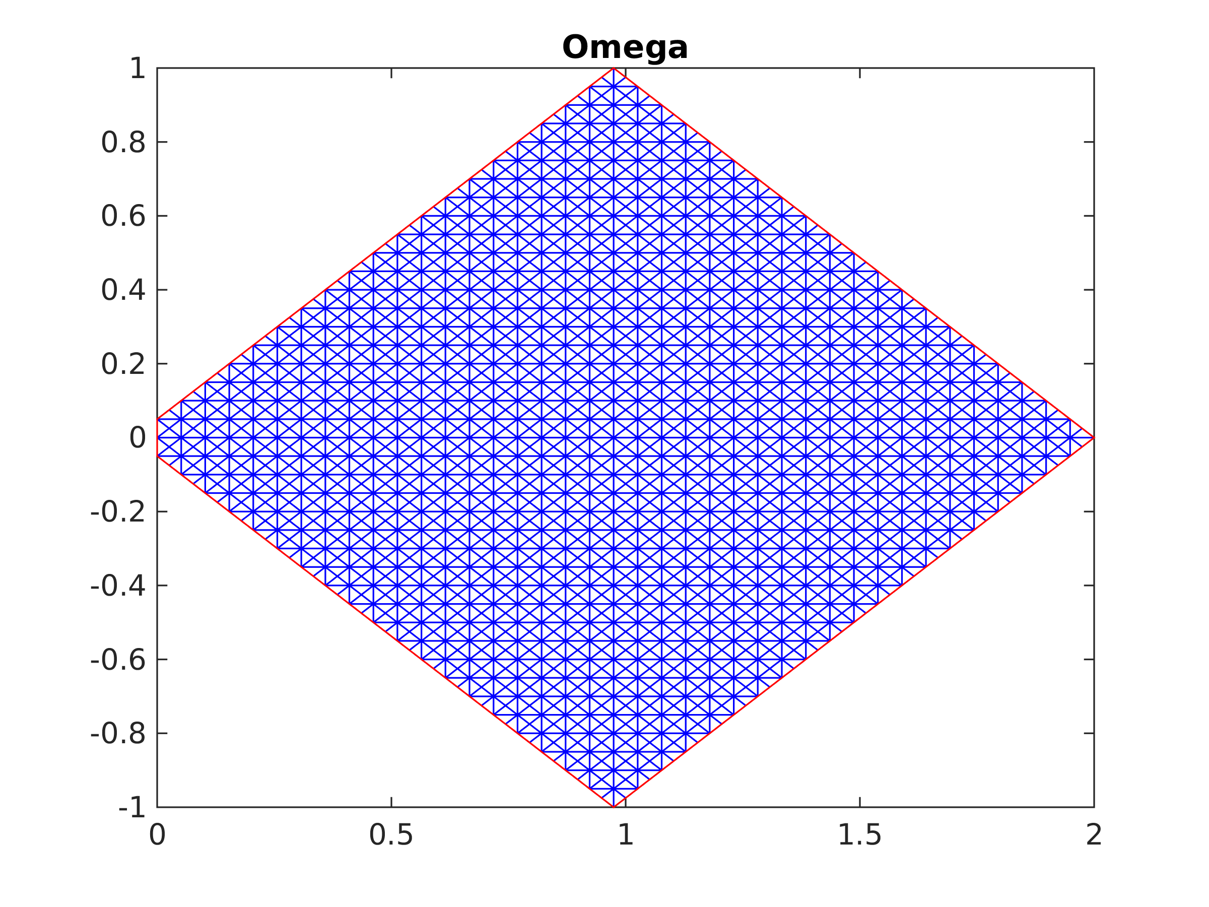
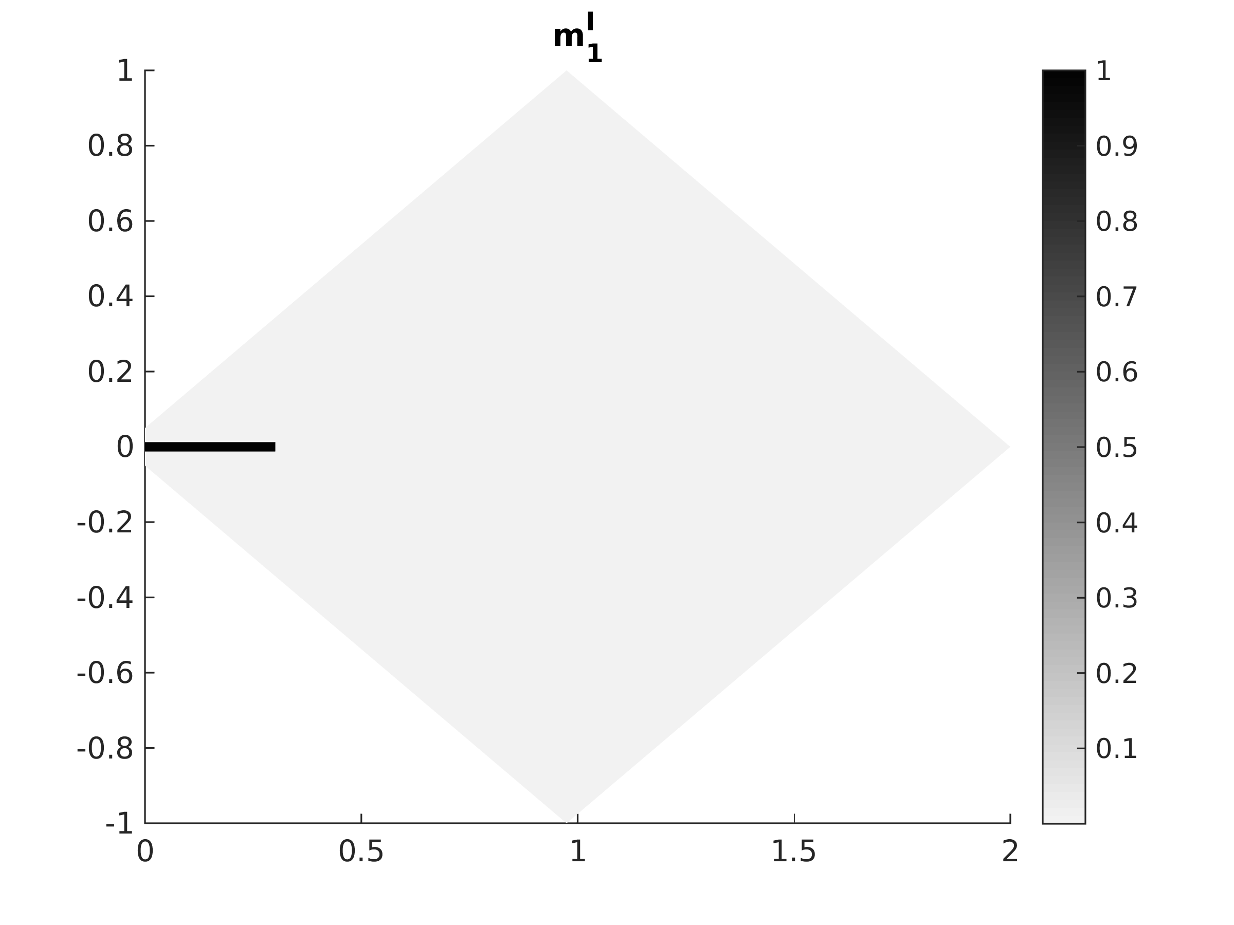
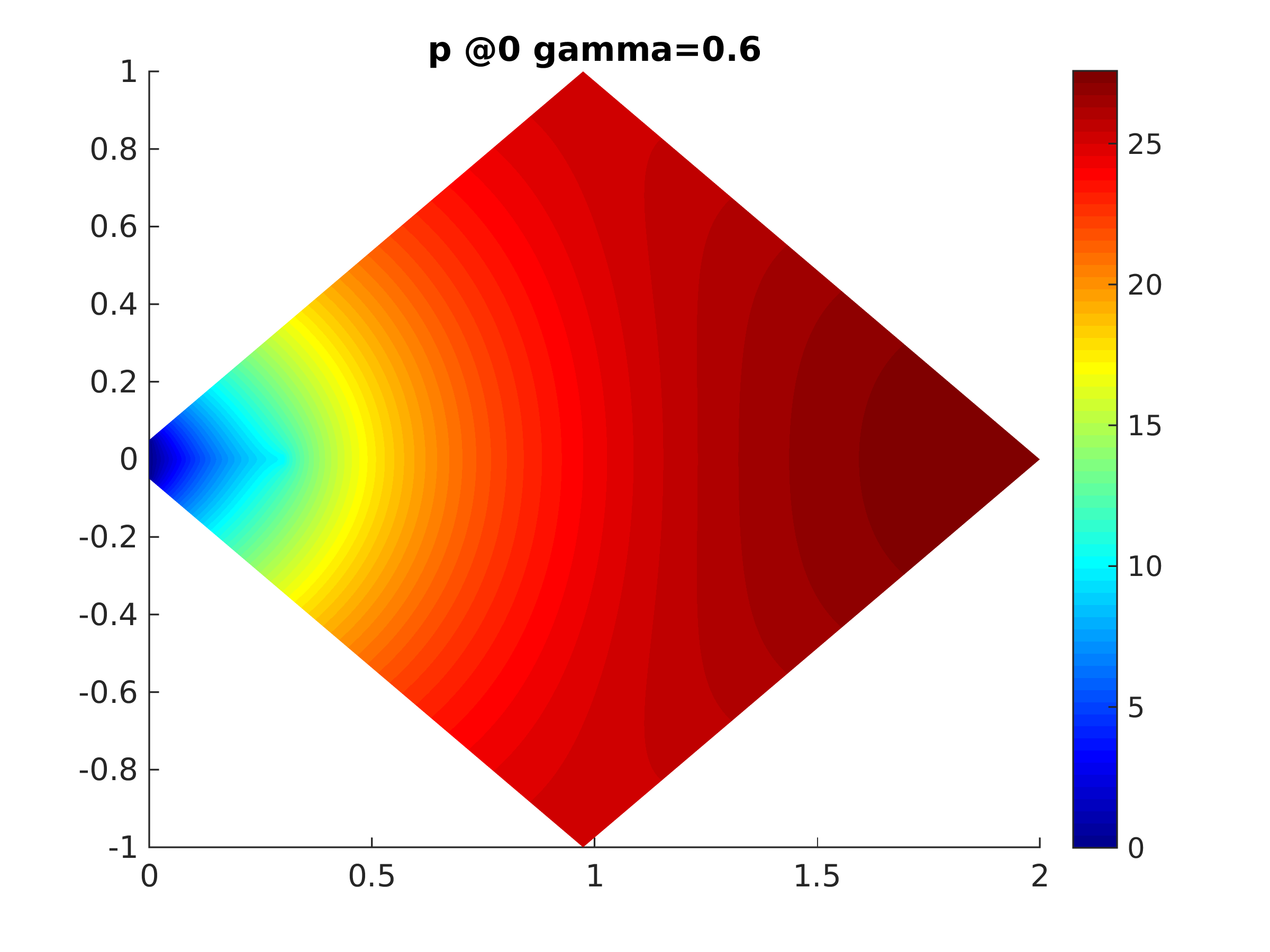
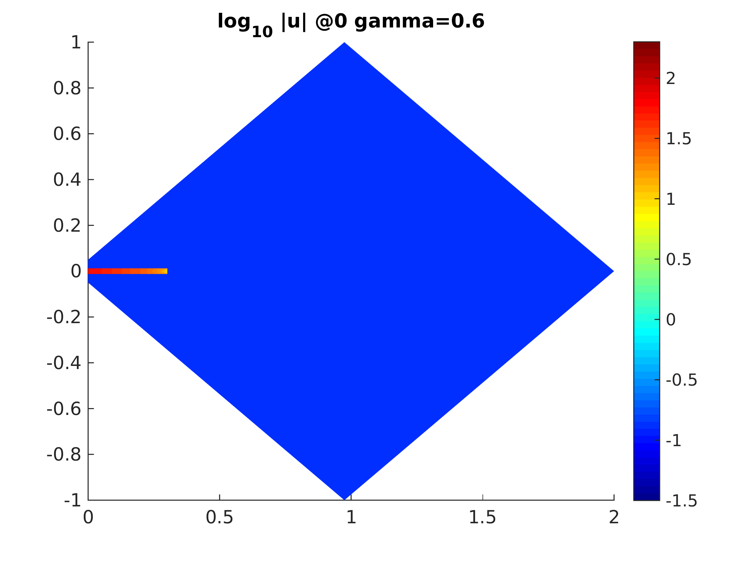
Figure 1: From left to right: Triangulation $\mathcal{T}_{h}$ of $\Omega$ with $1,678$ vertices and $3,196$ triangles; initial datum $m_{1}^{0}$, while $m_{2}^{0}=0$; initial pressure $p^{0}_{h}$; decadic logarithm of the absolute value of the initial velocity $|u^{0}_{h}|$. Note that $p^{0}_{h}$ and $|u^{0}_{h}|$ are the same for all values of $\gamma$.

As a computational domain we consider a diamond shaped two-dimensional domain with one edge cut, see Figure 1. We use a refined triangulation with $102,905$ vertices and $204,544$ triangles, which corresponds to $h\approx 0.0032$. The Dirichlet boundary is defined as $\Gamma=\{x\in\mathbb{R}^{2}:x_{1}=0\}\cap\partial\Omega$. If not stated otherwise, we let

$$S=1,\quad r=\frac{1}{10},\quad c=50,\quad D=\frac{1}{1000},\quad\gamma=\frac{1}{2},\quad\rho=10^{-12},$$

where $\rho$ is the regularization parameter defined in Section 5.1, and define the initial datum as

$$m^{0}_{1}(x)=\begin{cases}1,&x\leq 0.3\text{ and }|y|\leq 0.0125,\\ 0,&\text{ else,}\end{cases}\qquad m^{0}_{2}=0.$$

The main quantity of interest is the discrete velocity defined as

$$u_{h}^{k}=(rI+m_{h}^{k}\otimes m_{h}^{k})\nabla p_{h}^{k},$$

see also Section 4. The initial velocity $u_{h}^{0}$ and the initial pressure $p_{h}^{0}$ do not depend on $\gamma$ or $D$, and they are depicted in Figure 1. Since the numerical simulation is computationally expensive, we could not compute a stationary state in many examples below. However, in order to indicate that the presented solutions are near a stationary state, we define the stationarity measures

$$\mathcal{E}_{h,t}^{k}=\frac{\mathcal{E}_{h}(m^{k}_{h})-\mathcal{E}_{h}(m^{k-1}_{h})}{\delta^{k}}\quad\text{and}\quad m_{h,t}^{k}=\frac{\|m^{k}_{h}-m^{k-1}_{h}\|_{L^{2}(\Omega)}}{\delta^{k}}.$$

Furthermore, we define the quantity

$$s_{k}=\frac{\|u_{h}^{k}\|_{L^{2}(\Omega)}}{\|u_{h}^{k}\|_{L^{1}(\Omega)}},$$

which measures the sparsity of the network. In order to demonstrate the dependence of the solution on the different parameters in the system we first present some simulations for varying parameter values.

5.5 Varying $D$

The proliferation of the network and its structure is crucially influenced by diffusion. In the limit of vanishing diffusion $D=0$ the support of the conductance vector cannot grow. If diffusion is too large, interesting patterns will not show up in the stationary network. In the following we investigate the influence of different values for $D\in\{\frac{1}{2},\frac{1}{10},\frac{1}{100},\frac{1}{1000}\}$ on the network formation, while keeping $\gamma=1/2$ fixed. For $D\geq 1/10$, the obtained velocities are dominated by diffusion and no fine scale structures appear in the network, see Figures 2 and 3. For $D=1/100$ the resulting velocity is still diffusive, but some large scale structure is visible, see Figure 4. Decreasing the diffusion coefficient even further to $D=1/1000$, the network builds fine scale structures, see Figure 5. We note that the velocity is not near a stationary state here. For this very small $D=1/1000$, we have to be careful in interpreting the results. Our simulations have shown a strong mesh dependence for this case, which is not apparent for $D\geq 1/2$. We are not able to fully explain this behavior, but the comparison on different meshes for large diffusion and moderate values of $c$, which makes in turn $c\nabla p$ moderate, suggest that the mesh is too coarse to be able to resolve the diffusion process properly in the presence of strong activation. Here, one should use finer meshes to resolve this issue, which however also leads to prohibitively long computation times. A modification of the existing scheme to cope with this issue is left to further research.

Nonetheless, we believe that the velocities presented here are qualitatively correct, as they structurally show the right behavior, i.e. the smaller the diffusion $D$ the finer the scales in the network are, and the higher the sparsity index $s_{k}$ is, see also Table 1. Let us remark that the closer $\gamma$ is to $1/2$, the sparser the structures should be in a stationary state, which complies with the well-known fact that $L^{1}$-norm minimization promotes sparse solutions (note that the metabolic energy term in (1.5) becomes a multiple of $\left\|m\right\|_{L^{1}(\Omega)}$ for $\gamma=1/2$). Furthermore, even though the results in Figure 5 are quantitatively very different, they possess qualitatively the same properties; namely the thickness of the primary, secondary and tertiary branches. Let us again emphasize that the results of Figure 5 are far from being stationary, and the networks are likely to change their structure when further evolving.

Figure 2: Stationary velocity $|u_{h}^{k}|$ for $\gamma=\frac{1}{2}$ and $D=\frac{1}{2}$ in a Log₁₀-scale, and corresponding evolution of $\mathcal{E}_{h}(m_{h}^{k})$. The stationary state is reached for $t=3.2898$.

Figure 3: Near stationary velocity $|u_{h}^{k}|$ for $\gamma=\frac{1}{2}$ and $D=\frac{1}{10}$ in a Log₁₀-scale, and corresponding evolution of $\mathcal{E}_{h}(m_{h}^{k})$ and $\|c|\nabla p_{h}^{k}|\|_{L^{\infty}(\Omega)}$.

Figure 4: Near stationary velocity $|u_{h}^{k}|$ for $\gamma=\frac{1}{2}$ and $D=\frac{1}{100}$ in a Log₁₀-scale, and corresponding evolution of $\mathcal{E}_{h}(m_{h}^{k})$ and $\|c|\nabla p_{h}^{k}|\|_{L^{\infty}(\Omega)}$.

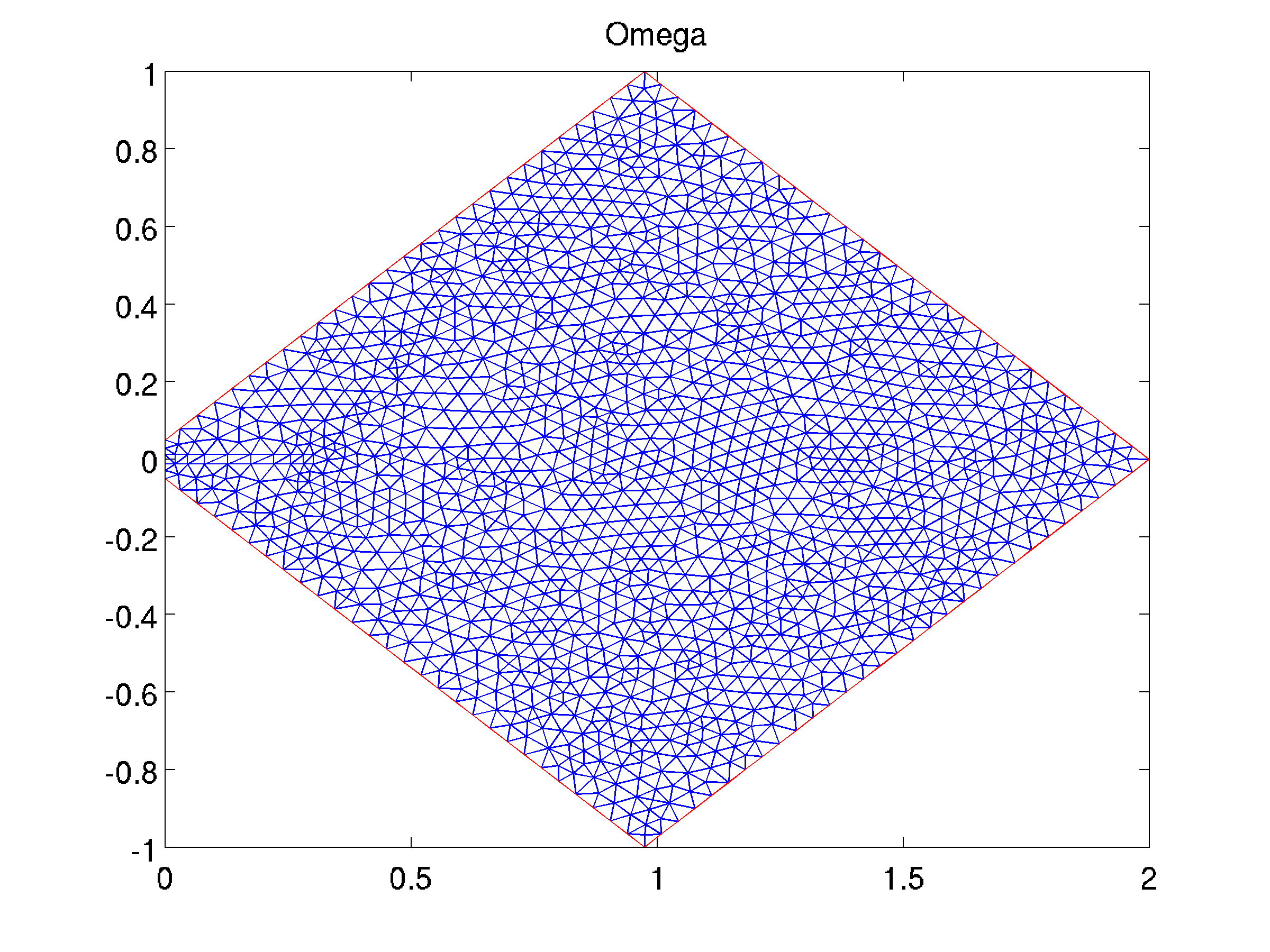
Figure 5: Left panel: Velocity $|u_{h}^{k}|$ for $\gamma=\frac{1}{2}$ and $D=\frac{1}{1000}$ in a Log₁₀-scale computed on a refined triangulation from the uniform grid shown in Figure 1 with $102,905$ vertices, cf. Section 5.4. Corresponding velocity (middle panel) computed on a refinement with $107,009$ vertices of the non-uniform grid shown in the right panel. For the refined non-uniform grid we have $\min h_{T}=0.0017$ and $\max h_{T}=0.0043$.

$D$	$\frac{1}{2}$	$\frac{1}{10}$	$\frac{1}{100}$
$t^{k}$	$3.2898$	$14.6883$	$32.333$
$\mathcal{E}_{h,t}^{k}$	$-1.1\times 10^{-5}$	$-2.9\times 10^{-6}$	$-1.5\times 10^{-2}$
$m_{h,t}^{k}$	$6.2\times 10^{-7}$	$4.5\times 10^{-2}$	$2.8\times 10^{-1}$
$s_{k}$	$1.344153$	$1.348375$	$1.576061$

Table 1: Stationarity and sparsity measures for different values of $D$ and $\gamma=\frac{1}{2}$, see Section 5.5.

5.6 Varying $\gamma$

In order to demonstrate the dependence of the network formation process on the relaxation term, we let $\gamma\in\{\frac{3}{5},\frac{3}{4},1,\frac{3}{2},2\}$; for $\gamma=\frac{1}{2}$ see Section 5.5. For $\gamma\in\{\frac{3}{2},2\}$ the results are depicted in Figure 9 and Figure 10. From the evolution of the energies and from Table 2 we may conclude that for these two values of $\gamma$ we are near a stationary state, and that for $\gamma>1$ no fine scale structures built up. For $\gamma=1$, depicted in Figure 8, network structures appear for large times. This may also be indicated by the oscillating behavior of $\nabla p$ for larger times. The changes in energy are however already small. In view of Section 4.2, stable solutions should satisfy $c\||\nabla p_{h}^{k}|\|_{L^{\infty}(\Omega)}\leq 1$ in the limiting case $D=0$. Here, $D=1/1000$, and $c|\nabla p_{h}^{k}|\leq 2$ is in accordance with this analysis.

For $\gamma\in\{\frac{3}{5},\frac{3}{4}\}$ we observe fine scale structures, which are depicted in Figure 6 and Figure 7. As remarked in the previous section, the network evolution is influenced by the underlying grid due to coarse discretization, very small diffusion, and very large activiation terms. Note that for small times we have $c\||\nabla p\|_{L^{\infty}(\Omega)}\approx 4000$, which enters quadratically in the activation term. The closer $\gamma$ is to $1$ the less the relaxation term promotes sparsity. This might explain that for $\gamma\geq\frac{3}{4}$ we see two branches originating from the Dirichlet boundary $\Gamma=\partial\Omega\cap\{x_{1}=0\}$. Since the pressure gradient is very large at the transition of Dirichlet to Neumann boundary, artificial conductance is created. Notice that these two branches do not appear for $\gamma\in\{\frac{1}{2},\frac{3}{5}\}$. In this context let us mention that in several situations $L^{1}$-type minimization can be performed exactly by soft-shrinkage, where values below a certain threshold, which corresponds to $\delta^{k}$ here, are set to $0$. Hence, small values of $m$, due to round-off or small diffusion, will less affect the evolution.

Figure 6: Near stationary velocity $|u_{h}^{k}|$ for $\gamma=\frac{3}{5}$, $D=\frac{1}{1000}$ in a Log₁₀-scale for different times, and corresponding evolution of the $\mathcal{E}_{h}(m_{h}^{k})$ and $\|c|\nabla p|\|_{L^{\infty}(\Omega)}$ vs. time in a logarithmic scaling.

Figure 7: Velocity $|u_{h}^{k}|$ for $\gamma=\frac{3}{4}$, $D=\frac{1}{1000}$ in a Log₁₀-scale, and corresponding evolution of the $\mathcal{E}_{h}(m_{h}^{k})$ and $\|c|\nabla p|\|_{L^{\infty}(\Omega)}$ vs. time in a logarithmic scaling.

Figure 8: Velocity $|u_{h}^{k}|$ for $\gamma=1$, $D=\frac{1}{1000}$ in a Log₁₀-scale, and corresponding evolution of the $\mathcal{E}_{h}(m_{h}^{k})$ and $\|c|\nabla p|\|_{L^{\infty}(\Omega)}$ vs. time in a logarithmic scaling.

Figure 9: Velocity $|u_{h}^{k}|$ for $\gamma=\frac{3}{2}$, $D=\frac{1}{1000}$ in a Log₁₀-scale, and corresponding evolution of the $\mathcal{E}_{h}(m_{h}^{k})$ and $\|c|\nabla p|\|_{L^{\infty}(\Omega)}$ vs. time in a logarithmic scaling.

Figure 10: Velocity $|u_{h}^{k}|$ for $\gamma=2$, $D=\frac{1}{1000}$ in a Log₁₀-scale, and corresponding evolution of the $\mathcal{E}_{h}(m_{h}^{k})$ and $\|c|\nabla p|\|_{L^{\infty}(\Omega)}$ vs. time in a logarithmic scaling.

$\gamma$	$\frac{3}{5}$	$\frac{3}{4}$	$1$	$\frac{3}{2}$	$2$
$t^{k}$	$121.5026$	$131.7063$	$140.3437$	$89.9778$	$95.1952$
$\mathcal{E}_{h,t}^{k}$	$-1.3\times 10^{-2}$	$-3.4\times 10^{-3}$	$-2.1\times 10^{-3}$	$-4.2\times 10^{-7}$	$-9.8\times 10^{-7}$
$m_{h,t}^{k}$	$2.1\times 10^{-1}$	$9.1\times 10^{-2}$	$1.1\times 10^{-1}$	$1.7\times 10^{-4}$	$1.1\times 10^{-5}$
$s_{k}$	$3.547262$	$4.153456$	$1.555159$	$1.181271$	$1.161117$

Table 2: Stationarity and sparsity measures for different values of $\gamma$ and $D=\frac{1}{1000}$, see Section 5.6. For $\gamma\in\{\frac{3}{2},2\}$ the change in the energy $\mathcal{E}_{h}$ is already within machine accuracy.

5.7 Unstable stationary solutions for $D=0$ and $\frac{1}{2}\leq\gamma<1$

In Section 4.3 we have constructed stationary solutions for $D=0$ and $\frac{1}{2}\leq\gamma<1$. In one dimension our stability analysis shows that these stationary states are not stable. In the following, we indicate that these stationary states are unstable also in two dimensions. To do so, we compute the minimizer of the functional $\mathcal{F}_{\alpha}$ defined in (4.18) with

$$\alpha=\alpha_{\gamma}=c^{-\frac{1}{4}}\Big{(}\frac{1-\gamma}{1+\gamma}\Big{)}^{\frac{\gamma-1}{2}},$$

which is (4.19) for general values of $c$. For the minimization we use a gradient descent method with step-sizes chosen by the Armijo rule [12]. The iteration is stopped as soon as two subsequent iterates of the pressure, say $p^{k}$ and $p^{k+1}$, satisfy $\|p^{k}-p^{k+1}\|_{H^{1}(\Omega)}/\|p^{k}\|_{H^{1}(\Omega)}<10^{-15}$, i.e. they coincide up to round-off errors. Since the derivative of $\mathcal{F}_{\alpha}$ is discontinuous, one should in general use more general methods from convex optimization to ensure convergence of the minimization scheme, for instance proximal point methods [14]. However, in our example also the gradient descent method converged. We set $\gamma=1/2$, $r=1$ and $c=50$. Moreover, we let $\mathcal{A}=\{x\in\mathbb{R}^{2}:(x_{1}-1)^{2}-x_{2}^{2}<1/4\}\subset\Omega$, see Figure 11. The stationary conductance $m_{0}$ is computed via (4.17) and satisfies

$$\|c\nabla p_{0}\otimes c\nabla p_{0}m_{0}-|m_{0}|^{2(\gamma-1)}m_{0}\|_{L^{2}(\Omega)}\approx 2\times 10^{-16},$$

which shows stationarity of the resulting solution $(p_{0},m_{0})$ up to machine precision. The resulting stationary pressure and conductances are depicted in Figure 11.

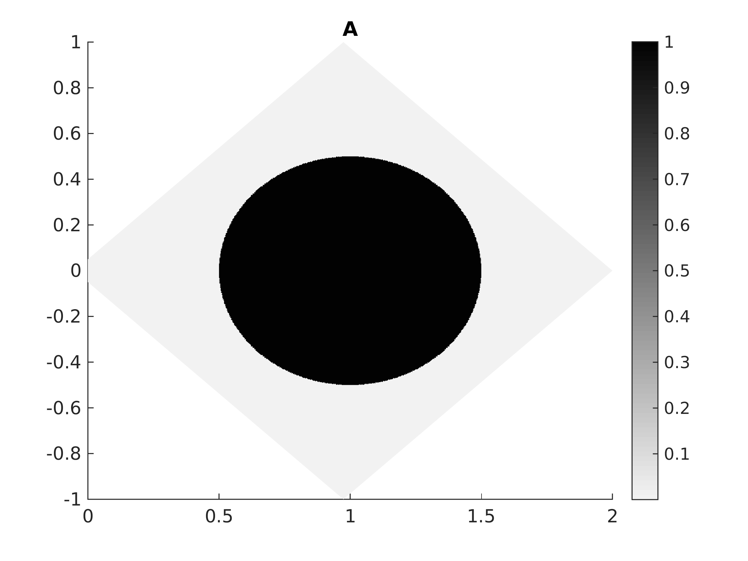
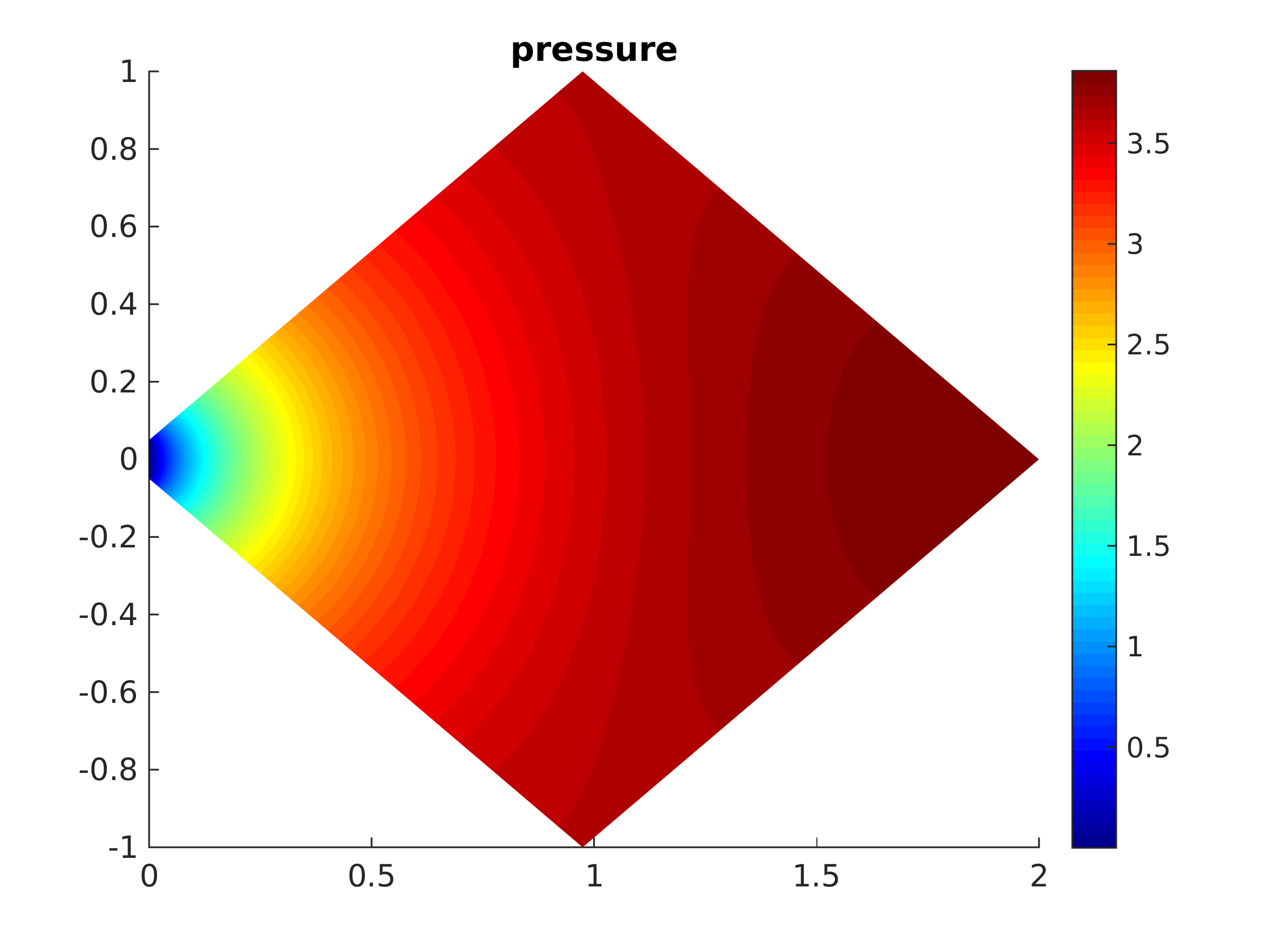
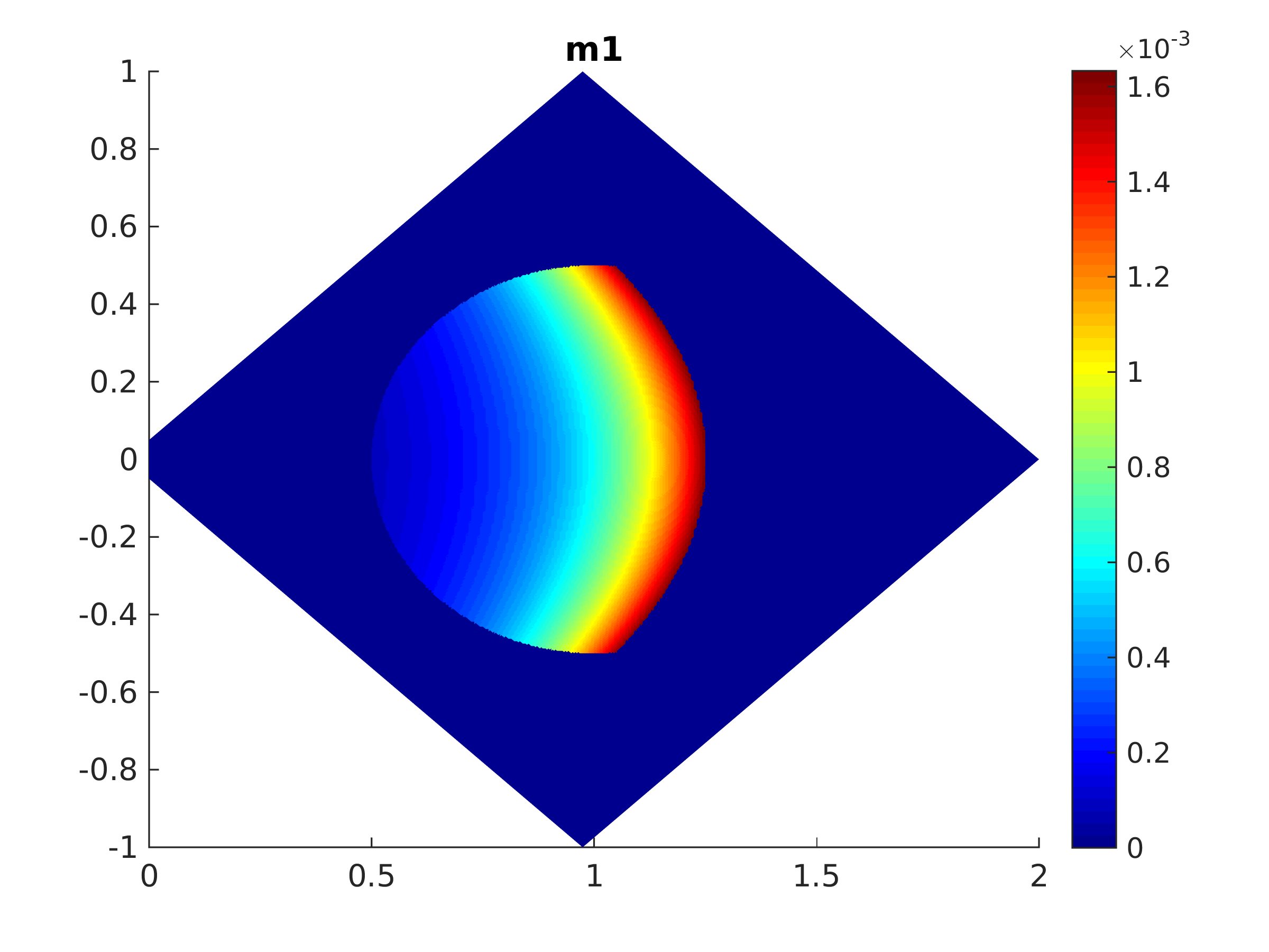
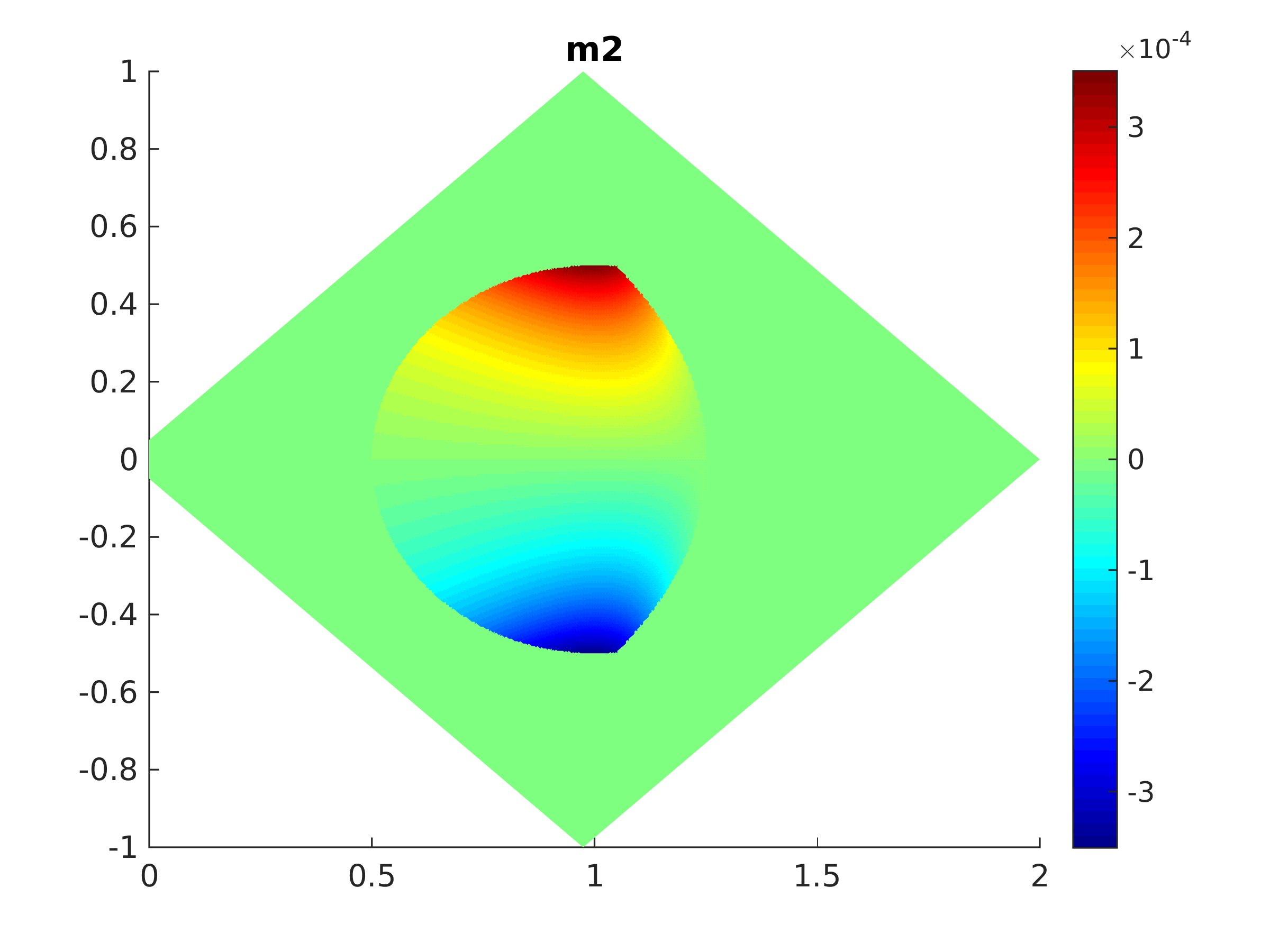
Figure 11: Stationary solution for $D=0$ and $\gamma=1/2$ via minimization of $\mathcal{F}_{\alpha}$ defined in (4.18). From left to right: Indicator function $\chi_{\mathcal{A}}$ of the set $\mathcal{A}$. Stationary pressure $p_{0}$. Stationary conductances $m_{0,1}$ and $m_{0,2}$.

In order to investigate the stability of the stationary state, we let $\eta$ denote uniformly distributed random noise on $[-\frac{1}{2},\frac{1}{2}]$, which we normalize such that $\|\eta\|_{L^{2}(\Omega)}=1$. We set

$$m^{0}_{\eta}=(1+\frac{\eta}{1000})m_{0}$$

as initial datum for our time-stepping scheme. The resulting evolution is depicted in Figure 12. Since the added noise is very small, the first picture in Figure 12 is visually identical to the absolute value $|m_{0}|$ of the unperturbed stationary solution. We observe that $m_{\eta}(t)$ does not converge to $m_{0}$, showing instability of the stationary state $(p_{0},m_{0})$.

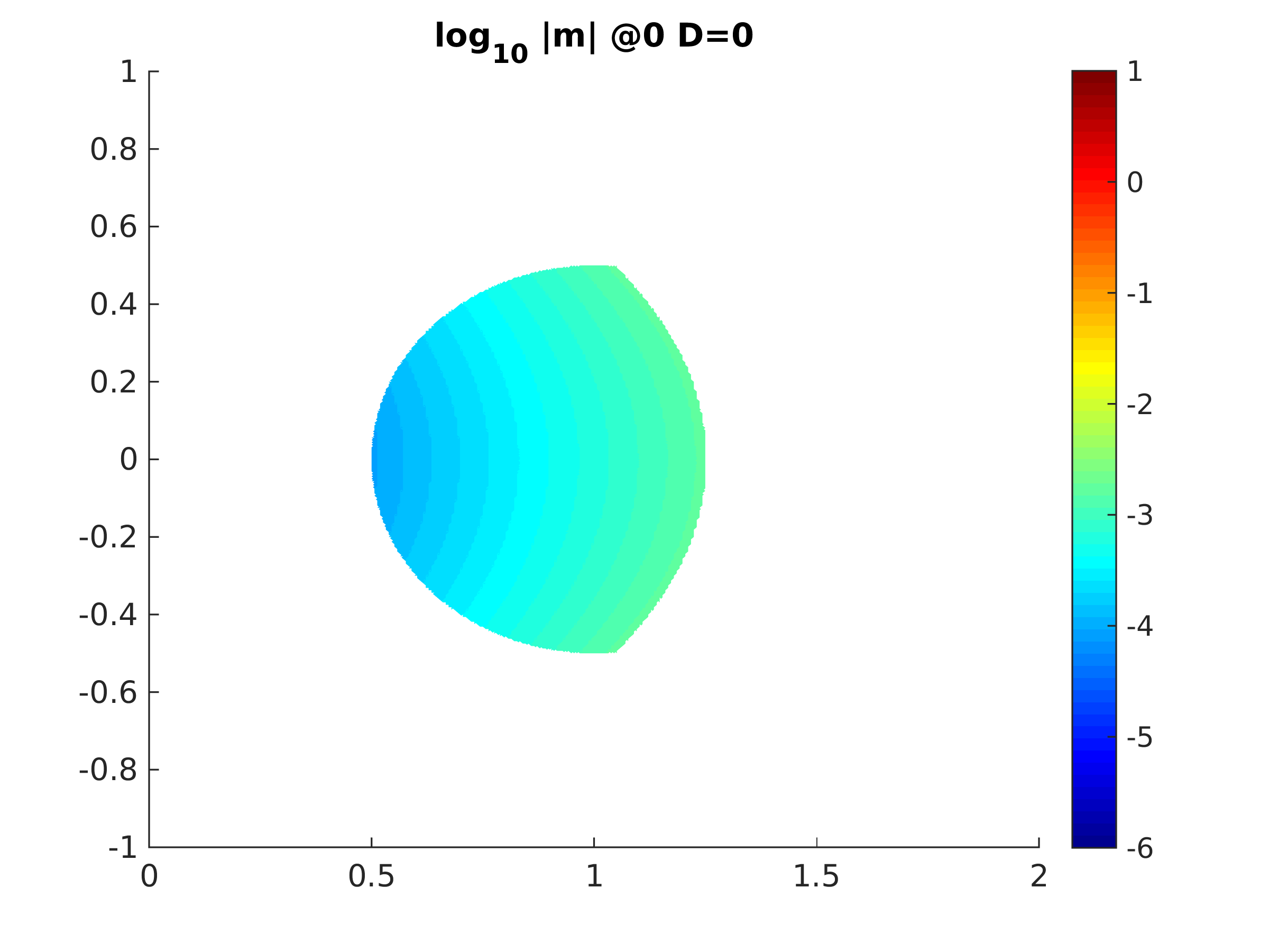
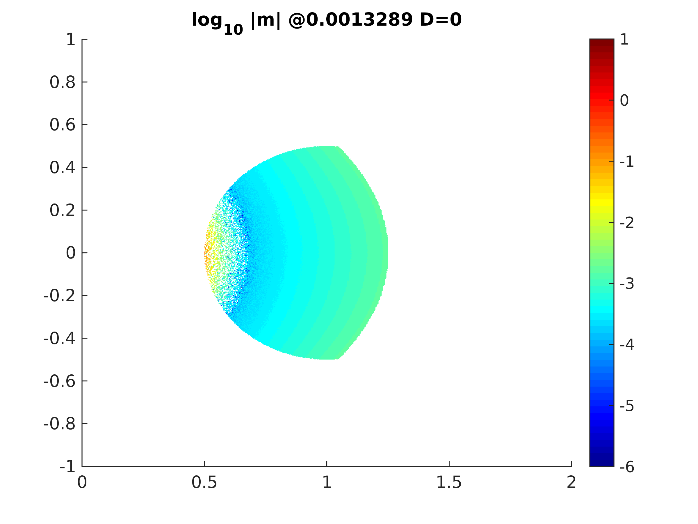
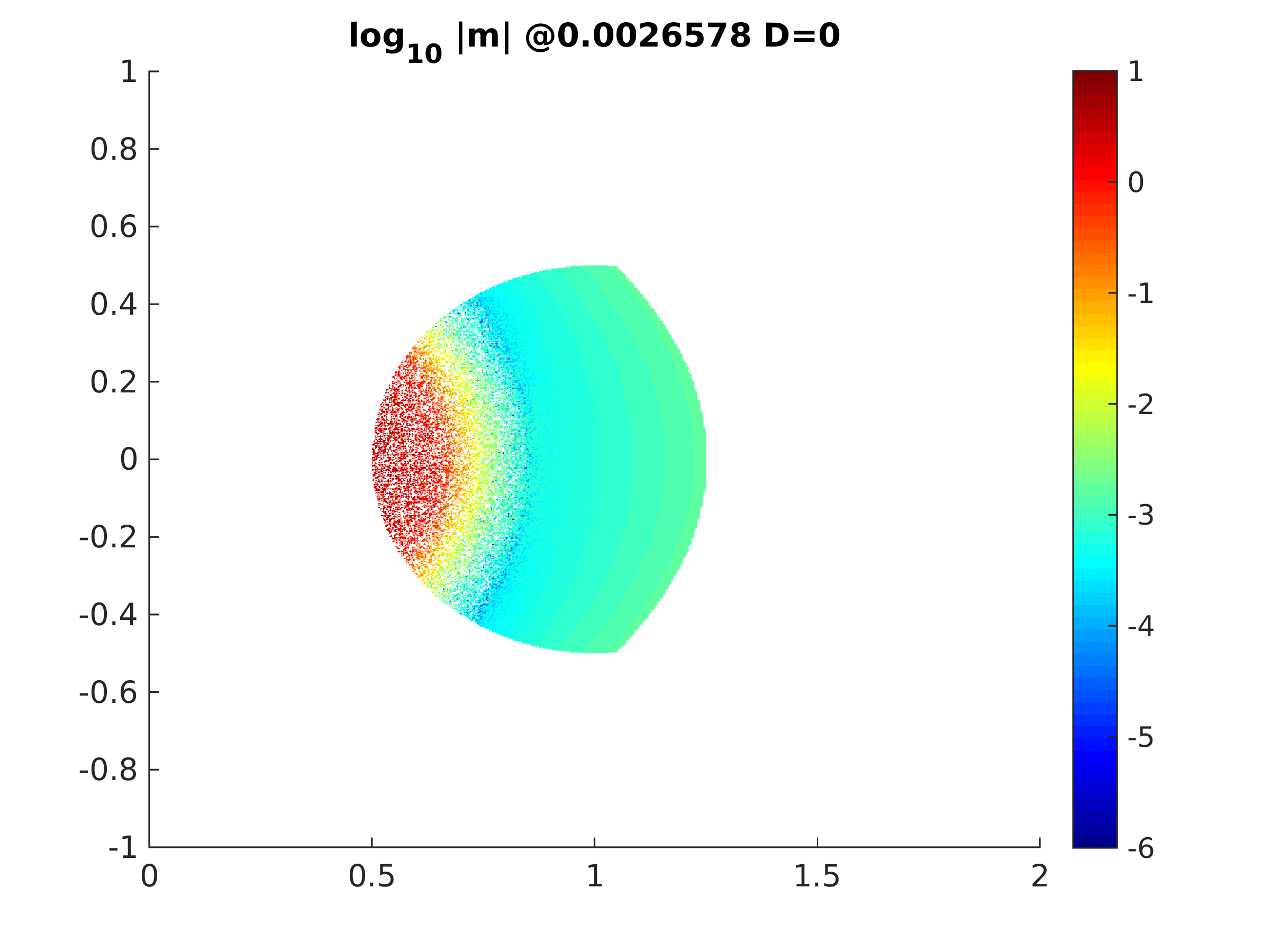
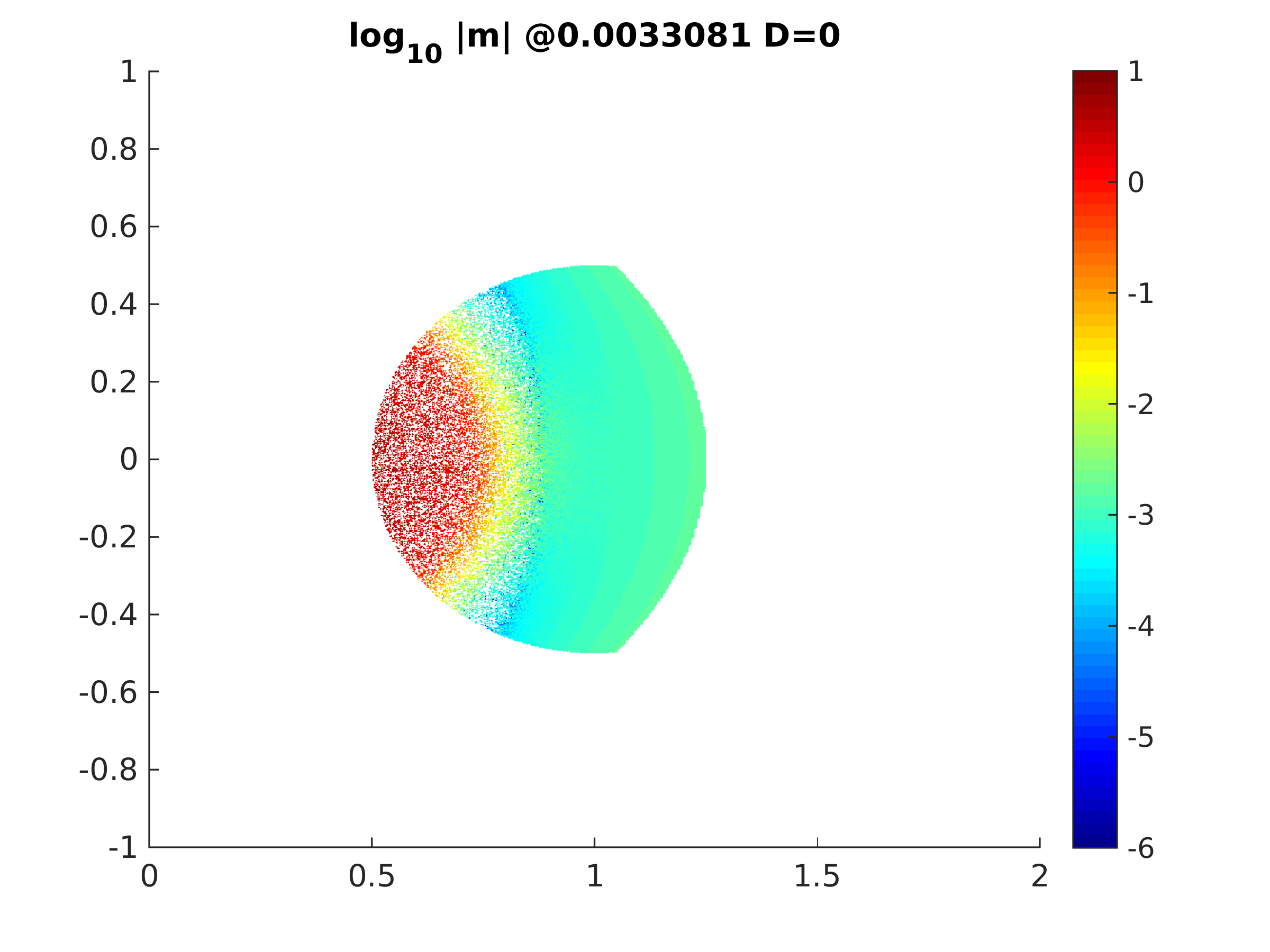
Figure 12: Evolution of the absolute value of the perturbed stationary solution $m^{0}_{\eta}$ computed in Section 5.7 for different times in a logarithmic scale.

5.8 Finite time break-down for $\gamma<1/2$

In Section 3.1 we have proven that $m$ decays exponentially to zero for $-1\leq\gamma\leq 1$, and that $m$ becomes zero after a finite time if $\gamma<1/2$ and the quantity $cS$ is sufficiently small. In this case, the relaxation term $|m|^{2(\gamma-1)}m$ develops a singularity and is meaningless in the limit $|m|\to 0$. In the following we demonstrate numerically that this happens also in two dimensions, which complements the one-dimensional analysis of Section 3.1. In view of Section 3.1, we replace the homogeneous Dirichlet conditions for $m$ by homogeneous Neumann conditions. For our test we set $c=1$ and $\rho=0$. To start with a strictly positive initial datum, we modify $m^{0}$ as follows

$$\tilde{m}^{0}_{1}=m^{0}_{1}+10^{-3},\quad\tilde{m}^{0}_{2}=m^{0}_{2},$$

and we define the extinction time as

$$T_{ex,\gamma}=\min\{t=t^{k}:\min_{x\in\Omega}|m_{h}^{k}(x)|<10^{-8}\}.$$

The results are depicted in Table 3. We observe that the smaller $\gamma$ the shorter the extinction time is. Monotone increase of $\gamma\mapsto T_{ex,\gamma}$ might be expected since for smaller values of $\gamma$ the relaxation term becomes more singular as $m\to 0$. Therefore, for smaller $\gamma$ the relaxation term dominates the activation term already for smaller times. In particular, $f_{\gamma,c}(m_{h}^{k},\nabla p_{h}^{k})$ acts like a sink. The threshold $10^{-8}$ seems to be somewhat arbitrary in the first place. However, in all our numerical simulations $\min_{x\in\Omega}|m_{h}^{k}(x)|$ decreased in a continuous fashion to values being approximately $10^{-6}$, and then dropped below the threshold in one step. Therefore, all threshold values in the interval $[10^{-8},10^{-6}]$ would yield the same $T_{ex,\gamma}$ in these examples. This result indicates that Lemma 4 might be extended to multiple dimensions.

$\gamma$	0	$\frac{1}{10}$	$\frac{1}{4}$	$\frac{2}{5}$
$T_{ex,\gamma}$	$5.3\times 10^{-7}$	$2.6\times 10^{-6}$	$2.1\times 10^{-5}$	$2.1\times 10^{-4}$
$\min_{x\in\Omega}|m_{h}^{k}(x)|$	$5.9\times 10^{-9}$	$5.4\times 10^{-9}$	$3.7\times 10^{-12}$	$2.8\times 10^{-10}$

Table 3: Extinction times $T_{ex,\gamma}$ for different values of $\gamma$.

Acknowledgment. BP is (partially) funded by the french ”ANR blanche” project Kibord: ANR-13-BS01-0004” and by Institut Universitaire de France. PM acknowledges support of the Fondation Sciences Mathematiques de Paris in form of his Excellence Chair 2011. MS acknowledges support by ERC via Grant EU FP 7 - ERC Consolidator Grant 615216 LifeInverse.

References

- [1] G. Albi, M. Artina, M. Fornasier and P. Markowich: Biological transportation networks: modeling and simulation. Preprint (2015).
- [2] J. Aubin, and A. Cellina: Differential Inclusions. Set Valued Maps and Viability Theory. Springer-Verlag Berlin Heidelberg New York Tokyo, 1984.
- [3] J. Àvila and A. Ponce: Variants of Kato’s inequality and removable singularities. Journal d’Analyse Mathématique 91 (2003), pp. 143–178.
- [4] D. Boffi, F. Brezzi, L. F. Demkowicz, R. G. Durán, R. S. Falk, and M. Fortin: Mixed Finite Elements, Compatibility Conditions, and Applications Springer, Berlin Heidelberg, 2008.
- [5] L. Caffarelli, and N. Riviere, The Lipschitz character of the stress tensor, when twisting an elastic plastic bar. Arch. Rational Mech. Anal. 69 (1979), no. 1, pp. 31–36.
- [6] L. C. Evans: Partial Differential Equations. American Mathematical Society, Providence, Rhode Island, 1998.
- [7] J. Haskovec, P. Markowich and B. Perthame: Mathematical Analysis of a PDE System for Biological Network Formation. Comm. PDE 40:5, pp. 918-956, 2015.
- [8] D. Hu: Optimization, Adaptation, and Initialization of Biological Transport Networks. Notes from lecture (2013).
- [9] D. Hu, private correspondence (2014).
- [10] D. Hu and D. Cai: Adaptation and Optimization of Biological Transport Networks. Phys. Rev. Lett. 111 (2013), 138701.
- [11] T. Koto: IMEX Runge-Kutta schemes for reaction-diffusion equations. Journal of Computational and Applied Mathematics (2008), Vol. 215, Issue 1, pp. 182–195.
- [12] J. Nocedal, and S. J. Wright: Numerical Optimization. Springer, New York, 1999.
- [13] R. Phelps: Lectures on Maximal Monotone Operators. Extracta Mathematicae 12 (1997), pp. 193-230.
- [14] R. T. Rockafellar: Monotone Operators and the Proximal Point Algorithm SIAM J. Control and Optimization (1976), Vol. 14, No. 5, pp. 877–898.
- [15] S. J. Ruuth: Implicit-explicit methods for reaction-diffusion problems in pattern formation. J. Math. Biol. (1995), 34:148–176.
- [16] M. Safdari: The regularity of some vector-valued variational inequalities with gradient constraints. arXiv:1501.05339.
- [17] M. Safdari: The free boundary of variational inequalities with gradient constraints. arXiv:1501.05337.