Hyperbolic chaos in self-oscillating systems based on mechanical triple linkage: Testing absence of tangencies of stable and unstable manifolds for phase trajectories

Abstract

Dynamical equations are formulated and a numerical study is provided for self-oscillatory model systems based on the triple linkage hinge mechanism of Thurston – Weeks – Hunt – MacKay. We consider systems with holonomic mechanical constraint of three rotators as well as systems, where three rotators interact by potential forces. We present and discuss some quantitative characteristics of the chaotic regimes (Lyapunov exponents, power spectrum). Chaotic dynamics of the models we consider are associated with hyperbolic attractors, at least, at relatively small supercriticality of the self-oscillating modes; that follows from numerical analysis of the distribution for angles of intersection of stable and unstable manifolds of phase trajectories on the attractors. In systems based on rotators with interacting potential the hyperbolicity is violated starting from a certain level of excitation.

MSC2010 numbers: 37D45, 37D20, 34D08, 32Q05, 70F20

Key words: dynamical system, chaos, hyperbolic attractor, Anosov dynamics, rotator, Lyapunov exponent, self-oscillator.

1 Introduction

Hyperbolic theory is a branch of the theory of dynamical systems undergoing essential and deep development during the last half century. It gives rigorous mathematical justification of chaotic behavior in deterministic systems, both in the discrete-time case (iterative maps – diffeomorphisms) and in continuous time (flows) [1, 2, 3, 4, 5]. The hyperbolic theory deals with invariant sets in phase space of dynamical systems composed exclusively of saddle trajectories. For such a trajectory, in the vector space of all possible infinitesimal perturbations (tangent space), one can define a subspace of vectors of exponentially decreasing norm in direct time, and a subspace of vectors exponentially decreasing in reverse time. In flow systems, for trajectories different from a fixed point, one has to introduce additionally a neutral one-dimensional subspace corresponding to perturbations along the phase trajectory, which neither grow, nor decay in time in average. An arbitrary vector of small perturbation is required to be a linear combination of vectors related to these subspaces. The set of trajectories that approach the reference orbit in the course of evolution in time is called the stable manifold. Similarly, the unstable manifold is a set of trajectories which approach the reference orbit in reverse time.

For conservative systems the hyperbolic chaos is associated with Anosov dynamics, when a typical trajectory in the phase space (for diffeomorphisms), or on the energy surface (for flows), is dense. For dissipative systems, the hyperbolic theory introduces a special type of chaotic attractors called the uniformly hyperbolic attractors.

The dynamic behavior considered by the hyperbolic theory is rough, or structurally stable, that is, the phase space arrangement, dynamical behavior and its statistical characteristics are not sensitive to variations in parameters and functions in the equations of motion. In this regard, it was natural to expect that the hyperbolic chaos should occur in many physical situations. However, as time passed and numerous examples of chaotic systems of different nature were proposed and studied, it became clear that they do not fit the narrow frames of the early hyperbolic theory. Therefore, the hyperbolic dynamics is regarded commonly rather as a kind of refined abstract image of chaos than something having direct relation to real systems. So, efforts of mathematicians were redirected to development of broadly applicable generalizations  [6, 7].

In textbooks and reviews on dynamical systems the hyperbolic chaos is represented usually by artificially constructed mathematical examples, like Anosov torus automorphism, DA-attractor of Smale, Smale – Williams solenoid, Plykin attractor  [1, 2, 3, 4, 5], whereas the question of implementation and possible applications of hyperbolic chaos in nature and technology was not elaborated for a long time.

If mathematicians are developing their examples using geometric, topological, algebraic constructions, a physicist should use a very different toolbox for design models with hyperbolic chaos: oscillators, particles, interactions, feedback loops etc. Recently, great progress has been made in this direction, and numerous examples of physically realizable systems are offered with attractors of Smale – Williams type and with other kinds of hyperbolic attractors [8, 9, 10, 11, 12, 13, 14, 15, 16, 17, 18, 19, 20]. Regarding clarity and transparency, a preference should be given surely to mechanical systems [20, 21, 22, 23, 24] as they are easily understood and interpreted through our everyday experience.

It may be noted, however, that the physical examples of hyperbolic attractors discussed so far [8, 9, 10, 11, 12, 13, 14, 15, 16, 17, 18, 19, 20] are obtained by reduction of the dynamical description to the Poincaré maps; in time intervals between the passages of the Poincaré section, one cannot speak definitely of uniform in time stretching and compression for the corresponding vector subspaces of perturbations. The question of design of physical systems with attractors, which would be characterized by hyperbolicity uniform in continuous time, at least approximately, remains open.

In this regard, an interesting starting point example is the hinge mechanism discussed in the popular-scientific article of Thurston and Weeks [25] as an illustration of a system with nontrivial topology of the configuration space. The mechanism is composed of three identical disks in a common plane, which are able to rotate about their central axes fixed at the vertices of an equilateral triangle (Fig. 1). At the edge of each disk a hinge is attached, and these hinges P_1,2,3 are connected by three identical rods to one more movable hinge P₀.

Instant configuration of the system is determined by the variables $\,\theta_{1},\,\theta_{2},\,\theta_{3}$ characterizing the rotation angles of the disks, but only two of them are independent because of the imposed constraint. Thus, the configuration space is a two-dimensional manifold. In settings we consider here it will be a surface of genus 3 (”pretzel with three holes”). The kinetic energy is a quadratic form of the generalized velocities (time derivatives of the local coordinates on the two-dimensional manifold). This quadratic form whose coefficients depend on lengths and masses of the structural elements, defines a certain metric on the two-dimensional manifold, and the motion takes place along the geodesic lines of this metric.

It was proven that for two-dimensional manifolds of genus different from 0 and 1 the dynamics along the geodesics are nonintegrable [26]. If the curvature is negative everywhere, the motion definitely corresponds to Anosov hyperbolic dynamics [27, 28]. In the triple linkage, as stated by Hunt and MacKay [29], with appropriate selection of sizes and masses one can reach a situation where the metric is of negative curvature over the whole manifold. Recently, some other hinge mechanisms capable of demonstrating the dynamics of Anosov have been proposed and analyzed [30, 31]. (Moreover, similar dynamics are discussed in the context of model description of motion of electrons in the doubly periodic potential of two-dimensional crystal lattice [32, 29].)

Hunt and MacKay also pointed out [29] that with addition of friction and providing feedback by means of a supplied control device one can get a hyperbolic chaotic attractor. However, in this respect, the authors limit themselves to though convincing, but only to verbal argumentation, appealing to the structural stability of the Anosov dynamics in the original conservative system. No study was carried out which would consider concrete equations of a model system, demonstrate hyperbolic chaos numerically, and analyze its quantitative characteristics like Lyapunov exponents.

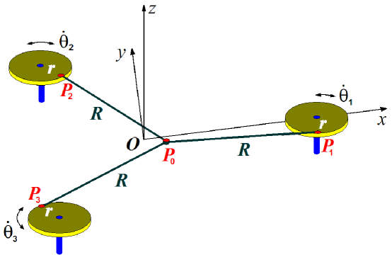
Figure 1: The triple linkage of Thurston and Weeks.

In the present article we formulate differential equations and provide a numerical study of self-oscillatory systems inspired by the triple linkage mechanism. The analysis here will be restricted to the case where the disk radius is small compared with the length of the rods connecting them with a movable hinge, and inertial properties of the mechanism are determined exclusively by the disks. In this case, the curvature of the metric defined by the kinetic energy is negative except for a finite set of eight points where it is zero. It is definitely enough to ensure the Anosov hyperbolic dynamics at any positive constant kinetic energy.

First, we will discuss a model precisely corresponding to the idea of Hunt and MacKay, when dissipation is introduced depending on the total kinetic energy of the system, being negative at small energies and positive at large energies; it creates a situation where some constant-energy surface becomes an attractor. Practically it implies that the added control device has to measure instantaneous kinetic energy of the whole system and actuators have to be introduced which provide application of torques to the disks to make the energy approach a desirable fixed value.

Another model system we examine is based on the assumption that each disk is a self-rotating subsystem; without interaction with the partners it would tend to rotation in one or other direction with some constant angular velocity not depending on specific initial conditions, due to the dissipation and feedback intrinsic to this subsystem itself. This variant seems much easier for practical implementation; it is possible to use a pair of friction clutches attached to each disk and passing rotation in opposite directions, with a properly chosen law of friction dependence on the relative angular velocity. When mechanical constraints are imposed by rods and hinges in such a device, the dynamics will not be reduced to that on a constant energy surface; the kinetic energy after decay of transients continues to oscillate chaotically.

Next, instead of the models with geometric constraints, we consider systems of three rotators interacting through some force field whose potential depends on the angles of rotation of the disks (see also Ref. [33]). The potential minimum is supposed to take place on a surface in the configuration space assumed in the previous models with mechanical constraint. It basically allows us to get away from the mechanical objects and to talk about possible implementation of chaotic systems of other physical nature, like electronic devices operating as generators of robust chaos.

As we depart from the original hinge mechanism, where chaos is hyperbolic, the hyperbolicity surely persists due to the structural stability of the Anosov dynamics for infinitesimal variations of the evolution operator in comparison with the original system. But for variations of finite magnitude, justification of the hyperbolic nature of the dynamics is of significance; so we have to apply some computer criteria for verification of hyperbolicity. In the present paper we will exploit the so-called criterion of angles for this purpose.

The idea of testing hyperbolicity based on statistics of angles between stable and unstable manifolds has been proposed for saddle invariant sets in [34]. Subsequently, it has been used for verification of hyperbolicity of attractors [35, 36], including attractors of Smale – Williams and Plykin type in Poincaré maps for systems that allow physical implementation [8, 13, 37].

The technique consists in the following. Along a typical phase trajectory belonging to the invariant set of interest, we follow it in forward time and in reverse time, and evaluate at each point an angle between the subspaces of perturbation vectors to analyze their statistical distribution. If the resulting distribution does not contain angles close to zero, it indicates a hyperbolic nature of the invariant set. If positive probability for zero angles is found, the tangencies between the stable and unstable manifolds of the trajectory do occur, and the invariant set is not hyperbolic. The latter may indicate the presence of a quasi-attractor that is a complex set, which contains long-period stable cycles with very narrow domains of attraction [2].

2 A system with a mechanical constraint
possessing an invariant energy surface

The Cartesian coordinates of the hinges P_1,2,3 attached to the disks (Figure 1) are expressed through the angles $\theta_{1}$, $\theta_{2}$, $\theta_{3}$, measured from the rays connecting the centers of the disks with origin O, as follows:

$$\begin{array}[]{l}x_{1}=1-r\cos\theta_{1},\,\,y_{1}=-r\sin\theta_{1},\\ x_{2}=-\textstyle{1\over 2}+\textstyle{1\over 2}r\cos\theta_{2}+\textstyle{{\sqrt{3}}\over 2}r\sin\theta_{2},\,\,\,\,y_{2}=\,\textstyle{{\sqrt{3}}\over 2}+\textstyle{1\over 2}r\sin\theta_{2}-\textstyle{{\sqrt{3}}\over 2}r\cos\theta_{2},\\ x_{3}=-\textstyle{1\over 2}+\textstyle{1\over 2}r\cos\theta_{3}-\textstyle{{\sqrt{3}}\over 2}r\sin\theta_{3},\,\,\,\,\,y_{3}=-\textstyle{{\sqrt{3}}\over 2}+\textstyle{1\over 2}r\sin\theta_{3}+\textstyle{{\sqrt{3}}\over 2}r\cos\theta_{3}.\\ \end{array}$$ (1)

The mechanical geometric constraint due to the rods and hinges implies that the radius of the circumscribed circle of the triangle P₁P₂P₃ must be $R$. By the well-known formula, $R=abc/4S$, where $a$, $b$, $c$ are the lengths of sides of the triangle, and $S$ is its area. With given coordinates of three vertices ($x_{i}$, $y_{i})$, we evaluate the lengths of sides, and the area is expressed through the vector product of two vectors, one from P₁ to P₂ and the other from P₁ to P₃: $S=\textstyle{1\over 2}\left|{{\rm{\bf b}}\times{\rm{\bf c}}}\right|$. Thus, we have $(abc)^{2}-4R^{2}({\rm{\bf b}}\times{\rm{\bf c}})^{2}=0$, which can be rewritten as

$$\begin{array}[]{l}[(x_{1}-x_{2})^{2}+(y_{1}-y_{2})^{2}][(x_{2}-x_{3})^{2}+(y_{2}-y_{3})^{2}][(x_{3}-x_{1})^{2}+(y_{3}-y_{1})^{2}]-\\ \,\,\,\,\,\,\,\,\,\,\,\,\,\,\,\,\,\,\,\,\,\,\,-4R^{2}(x_{2}y_{3}+x_{3}y_{1}+x_{1}y_{2}-x_{3}y_{2}-x_{1}y_{3}-x_{2}y_{1})^{2}=0.\\ \end{array}$$ (2)

Substituting the expressions (1), we get the geometric constraint equation in the form $F(\theta_{1},\theta_{2},\theta_{3})=0$.

Let us suppose that the disks are the only massive elements of the construction, and their moments of inertia are assumed to be unity; additionally, each of them may be driven by an external torque $M_{1,2,3}$. Then the equations of motion read (see, e.g., [38, 39])

$$\ddot{\theta}_{1}=M_{1}+\Lambda\partial F/\partial\theta_{1},\,\,\ddot{\theta}_{2}=M_{1}+\Lambda\partial F/\partial\theta_{2},\,\,\ddot{\theta}_{3}=M_{3}+\Lambda\partial F/\partial\theta_{3},$$ (3)

$$F(\theta_{1},\,\,\theta_{2},\,\,\theta_{3})=0,$$ (4)

where the multiplier $\Lambda$ must be determined taking into account the algebraic condition of the holonomic mechanical constraint (4). This expression $F=0$ and the relation obtained by differentiating $\sum\nolimits_{j=1}^{3}{\dot{\theta}_{j}}\partial F/\partial\theta_{j}=0$ correspond to two integrals of motion for the system (3), which is formally of the sixth order.

Assuming $r<<1$ and expanding (2) in Taylor series up to terms of the first order in the small parameter, we obtain

$$27(R^{2}-1)-18r(2R^{2}-3)(\cos\theta_{1}+\cos\theta_{2}+\cos\theta_{3})=0.$$ (5)

Setting $R$=1,we arrive at a very simple equation of holonomic constraint

$$F(\theta_{1},\theta_{2},\theta_{3})=\cos\theta_{1}+\cos\theta_{2}+\cos\theta_{3}=0,$$ (6)

which will be the only one used in subsequent considerations.

In the conservative case, in the absence of the external torques, $M_{1,2,3}$=0, the system conserves the kinetic energy

$$T=\textstyle{1\over 2}(\dot{\theta}_{1}^{2}+\dot{\theta}_{2}^{2}+\dot{\theta}_{3}^{2}),$$ (7)

and the dynamics can be interpreted as motion of a point particle on a two-dimensional surface given by equation (6), along the geodesics of the metric defined by the quadratic form

$$ds^{2}=\textstyle{1\over 2}(d\theta_{1}^{2}+d\theta_{2}^{2}+d\theta_{3}^{2}),$$ (8)

with the consistence condition on the differentials $d\theta_{1}\sin\theta_{1}+d\theta_{2}\sin\theta_{2}+d\theta_{3}\sin\theta_{3}=0$ because of the constraint equation. Calculation of the Gaussian curvature leads to the formula [29, 33]

$$K=-\frac{\cos^{2}\theta_{1}+\cos^{2}\theta_{2}+\cos^{2}\theta_{3}}{2\left({\sin^{2}\theta_{1}+\sin^{2}\theta_{2}+\sin^{2}\theta_{3}}\right)^{2}}.$$ (9)

As is seen, the curvature is negative everywhere, except for a finite number of points, namely, eight of them, where it vanishes: $(\theta_{1},\,\theta_{2},\,\theta_{3})=(\pm\pi/2,\,\pm\pi/2,\,\pm\pi/2)$. Therefore, the motion along geodesic lines with nonzero kinetic energy is the Anosov dynamics [29].

Formally, the phase space of the system is six-dimensional; accordingly, there are six Lyapunov exponents characterizing the behavior of phase trajectories perturbed near a reference orbit. In the conservative case, there is one positive, four zero, and one negative exponent, which is equal to the positive exponent in absolute value. One exponent equal to zero appears due to the autonomous nature of the system; it is responsible for a perturbation vector tangent to the reference phase trajectory. One more zero exponent is associated with a perturbation corresponding to the energy shift. The remaining two zero exponents are nonphysical and should be excluded from consideration, since they relate to perturbations of two integrals of motion caused by the mechanical constraint, i.e., they violate the constraint equation.

Since the system does not have any intrinsic characteristic time scale, the positive and negative Lyapunov exponents for the exponential growth and decay of perturbations per unit time should be proportional to the velocity, i.e., to the square root of energy, namely, $\lambda=\pm\kappa\sqrt{W}$. As the dynamics is associated with motion on the surface of negative curvature, the coefficient in this expression is determined by the average curvature of the metric. Empirical numerical calculations for the system with the constraint (6) yield $\kappa=0.70$ [33].

To get a dissipative system with chaotic attractor according to the proposals of Hunt and MacKay [29], we introduce the torques depending on the generalized velocities in such a way that the kinetic energy tends during the time evolution to a value $\mu$, namely

$$M_{i}=\nu[\mu-\textstyle{1\over 2}(\dot{\theta}_{1}^{2}+\dot{\theta}_{2}^{2}+\dot{\theta}_{3}^{2})]\dot{\theta}_{i},\,\,i=1,2,3,$$ (10)

where $\nu$ is a constant factor. To obtain such a function, the mechanism should be supplemented with a controlling device and actuators, which apply the torques $M_{1,2,3}$ to the axles of the disks depending on the value of the detected instant kinetic energy.

Differentiating the constraint equation with respect to time once and twice, we have

$$\begin{array}[]{c}\dot{\theta}_{1}\sin\theta_{1}+\dot{\theta}_{2}\sin\theta_{2}+\dot{\theta}_{3}\sin\theta_{3}=0,\\ \ddot{\theta}_{1}\sin\theta_{1}+\ddot{\theta}_{2}\sin\theta_{2}+\ddot{\theta}_{3}\sin\theta_{3}+\dot{\theta}_{1}^{2}\cos\theta_{1}+\dot{\theta}_{2}^{2}\cos\theta_{2}+\dot{\theta}_{3}^{2}\cos\theta_{3}=0.\\ \end{array}$$ (11)

Substituting the second derivatives from the equations of motion (3) into (11), we obtain an explicit formula for the multiplier

$$\Lambda=-\frac{\sum\nolimits_{j=1}^{3}{\left({\dot{\theta}_{j}^{2}\cos\theta_{j}+M_{j}\sin\theta_{j}}\right)}}{\sum\nolimits_{j=1}^{3}{\sin^{2}\theta_{j}}},$$ (12)

and arrive at the closed set of equations

$$\ddot{\theta}_{i}=\nu[\mu-\textstyle{1\over 2}(\dot{\theta}_{1}^{2}+\dot{\theta}_{2}^{2}+\dot{\theta}_{3}^{2})]\left({\dot{\theta}_{i}-\frac{\sum\nolimits_{j=1}^{3}{\dot{\theta}_{j}\sin\theta_{j}}}{\sum\nolimits_{j=1}^{3}{\sin^{2}\theta_{j}}}\sin\theta_{i}}\right)-\frac{\sum\nolimits_{j=1}^{3}{\dot{\theta}_{j}^{2}\cos\theta_{j}}}{\sum\nolimits_{j=1}^{3}{\sin^{2}\theta_{j}}}\sin\theta_{i},\,\,i=1,2,3.$$ (13)

The equation determining the time evolution of the kinetic energy $W=\textstyle{1\over 2}(\dot{\theta}_{1}^{2}+\dot{\theta}_{2}^{2}+\dot{\theta}_{3}^{2})$ is derived easily from (13) and reads

$$\dot{W}=2\nu(\mu-W)W.$$ (14)

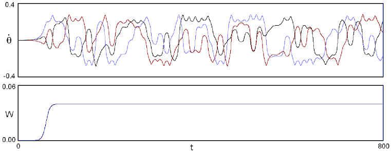
Figure 2: Dependences of the generalized velocities $\dot{\theta}_{1},\,\,\dot{\theta}_{2},\,\,\dot{\theta}_{3}$ and the energy $W$ on time in the course of the transient process from a low-energy state towards chaotic self-oscillations in the system (13) at $\mu=0.04$, $\nu=3$.

Figure 2 illustrates the transient process in the system (13) at $\mu$=0.04 and $\nu$=3 starting from a point in the configuration space consistent with the mechanical constraint with very small initial velocity towards the regime of chaotic self-oscillations, which corresponds to constant energy, although the angular velocities behave chaotically, without any visible repetition of forms.

Figure 3 shows a trajectory in the configuration space obtained from numerical integration of equations (13). Due to the imposed mechanical constraint, it is placed on a two-dimensional surface defined by the equation $\cos\theta_{1}+\cos\theta_{2}+\cos\theta_{3}=0$. When plotting the picture, the angular variables are related to the interval from 0 to 2$\pi$, i.e., the diagram in the three-dimensional space ($\theta_{1}$,$\theta_{2}$,$\theta_{3})$ corresponds to a single fundamental cubic cell, which reproduces itself periodically with a shift by 2$\pi$ along each of three coordinate axes. Any opposite pair of faces of the cubic cell may be identified; then we come to a compact manifold of genus 3, i.e., to the surface topologically equivalent to the ”pretzel with three holes.”

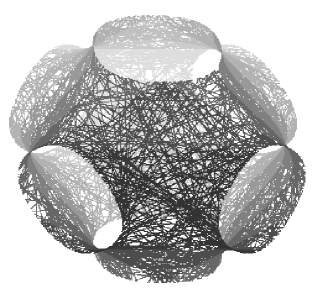
Figure 3: A trajectory in three-dimensional configuration space of the system (13) obtained by numerical integration of the equations; it is placed on the two-dimensional surface defined by the constraint equation $\cos\theta_{1}+\cos\theta_{2}+\cos\theta_{3}=0$.

In order to characterize the observed chaos quantitatively, we turn to the Lyapunov exponents. Excluding two nonphysical zero exponents, which violate the constraint equation, we have four exponents in the rest. Since the motion on the attractor takes place on the energy surface, the exponents for perturbations without departure from this surface will be equal to those in the conservative system at the same energy: $\kappa\sqrt{W}$, 0, and $-\kappa\sqrt{W}$. The exponent corresponding to perturbation of the energy is evaluated simply as the Lyapunov exponent of the attracting fixed point $W=\mu$ in the equation (14); it is equal to $-2\nu\mu$.

Figure 4 shows graphs for the Lyapunov exponents versus parameter $\mu$ in the system (13). The solid lines correspond to the relations mentioned in the preceding paragraph. The dots represent results of calculation of the Lyapunov exponents using the Benettin algorithm [40, 13]. Numerical integration of equations (13), formally written in the form ${\rm{\bf\dot{x}}}={\rm{\bf F}}({\rm{\bf x}},t)$, where x is a six-dimensional state vector, is performed together with a collection of six sets of variation equations ${\rm{\bf\dot{\tilde{x}}}}={\rm{\bf{F}^{\prime}}}({\rm{\bf x}}(t),t){\rm{\bf\tilde{x}}}$, where ${\rm{\bf{F}^{\prime}}}({\rm{\bf x}}(t),t)$ is the Jacobi matrix of size 6x6 composed of partial derivatives. In the process of numerical integration, orthogonalization and normalization of the perturbation vectors is carried out at each step, according to the Gram – Schmidt procedure. Lyapunov exponents are evaluated as coefficients of increase or decrease of the accumulated sums of logarithms of vector norms obtained after the orthogonalization, but before the normalization. At the final stage of the procedure, two nonphysical exponents violating the mechanical constraint condition are excluded.

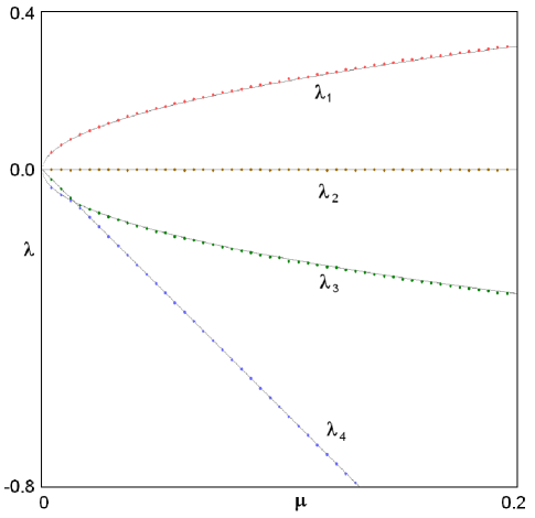
Figure 4: Lyapunov exponents for the dissipative system (13) depending on the parameter $\mu$ at $\nu$=3. The dots correspond to numerical computations based on the Benettin algorithm, and the solid lines are plotted according to the formulas $\pm 0.70\sqrt{\mu}$ and $-2\nu\mu$.

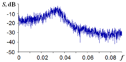
Figure 5: The power spectrum of the signal $u(t)=\cos\theta_{1}(t)$ from the system (13) for $\nu$ = 3, $\mu$ = 0.04

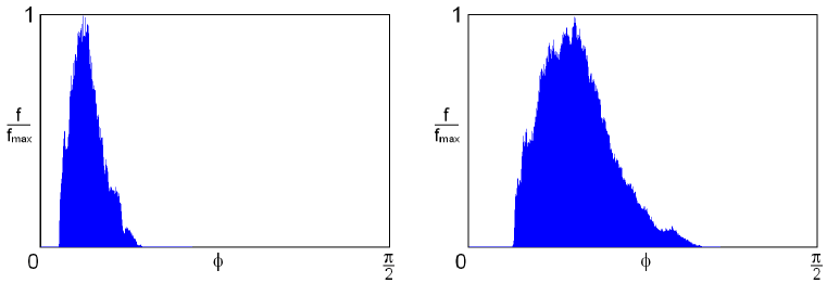
Figure 6: Verification of the criterion of angles in the system (13) with a mechanical constraint for the attractor represented by an invariant energy surface at $\mu$=0.04 (a) and at $\mu$=0.25 (b) with $\nu$=3.

Figure 5 shows the power spectrum of the signal determined as $u(t)=\cos\theta_{1}(t)$. It is obtained by processing time series from numerical simulation of the dynamics on the attractor at $\mu$ = 0.04 and $\nu$ = 3. The spectrum is computed in accordance with the procedure of the power spectral density estimation recommended in the theory of stochastic processes [41]. The spectral density is depicted in logarithmic scale, in decibels (10 dB correspond to the 10-fold ratio of power levels). As seen from the diagram, the continuous spectrum, which corresponds to chaotic dynamics, is quite uniform (no pronounced peaks are seen).

The observed attractor is undoubtedly hyperbolic since the dynamics takes place along geodesic lines of the metric of negative curvature (except a finite number of points) on the energy surface. It is interesting, however, to try application of the criterion of angles in this case to test the methodology, which further will be exploited in situations where the presence or absence of hyperbolicity is not trivial.

To use the criterion in a form proposed in [37], we start by calculating a reference orbit ${\rm{\bf x}}(t)$ on the attractor, tracing the solution of the equation ${\rm{\bf\dot{x}}}={\rm{\bf F}}({\rm{\bf x}},t)$ over a sufficiently long time interval. Then take the linearized equation for the perturbation vector ${\rm{\bf\dot{\tilde{x}}}}={\rm{\bf{F}^{\prime}}}({\rm{\bf x}}(t),t){\rm{\bf\tilde{x}}}$ and integrate it along the reference trajectory forward in time with normalization of the vector ${\rm{\bf\tilde{x}}}$ at each step $n$ to avoid divergence. (In our problem we have one unstable direction, and, so, one positive Lyapunov exponent.) The result is a set of unit vectors $\,\{{\rm{\bf x}}_{n}\}$. Next, the integration is performed in reverse time along the same reference orbit using the linear equation ${\rm{\bf\dot{u}}}=-[{\rm{\bf{F}^{\prime}}}({\rm{\bf x}}(t),t)]^{\rm{T}}{\rm{\bf u}}$, where the superscript T denotes the matrix conjugation. It provides a set of vectors $\,\{{\rm{\bf u}}_{n}\}$, each defines the orthogonal complement to the stable subspace of the perturbation vectors at a point of the reference trajectory. These vectors also are normalized to unity in the course of the computations. Now, to evaluate the angle $\phi$ between the one-dimensional unstable subspace and the stable subspace at each $n$-th step we calculate the angle $\beta_{n}\in$[0,$\pi$/2] between the vectors ${\rm{\bf\tilde{x}}}_{n}$ and ${\rm{\bf u}}_{n}$: $\cos\beta_{n}=\left|{{\rm{\bf u}}_{n}(t)\cdot{\rm{\bf\tilde{x}}}_{n}(t)}\right|$, and set $\phi_{n}=\pi\mathord{\left/{\vphantom{\pi 2}}\right.\kern-1.2pt}2-\beta_{n}$.

Figure 6 shows the histograms obtained numerically for the angles between stable and unstable subspaces in the system (13). As is seen, the distributions are well separated from zero angles $\phi$, i.e., the test confirms the hyperbolic nature of the attractor.

3 A system of three self-rotators
with a mechanical constraint

Let us turn now to a system where the external forces applied to the disks depend only on the angular velocity of each disk, namely, suppose

$$M_{i}=\nu(\mu-\textstyle{1\over 2}\dot{\theta}_{1}^{2})\dot{\theta}_{i},\,\,i=1,2,3.$$ (15)

In a real device, to provide such torques, one can use a pair of friction clutches attached to each disk, which transmit oppositely directed rotations, selecting properly the functional dependence of the friction coefficient on the velocity. In this case, each of the three disks is a self-rotator that means a subsystem, which, being singled out, manifests evolution in time with approach to a steady rotation with constant angular velocity $\dot{\theta}=\pm\sqrt{2\mu}$ in one or other direction (depending on initial conditions).

Equations (3) upon the constraint (4) in this case can be rewritten as

$$\ddot{\theta}_{i}=\nu(\mu-\textstyle{1\over 2}\dot{\theta}^{2})\left({\dot{\theta}_{i}-\frac{\sum\nolimits_{j=1}^{3}{\dot{\theta}_{j}\sin\theta_{j}}}{\sum\nolimits_{j=1}^{3}{\sin^{2}\theta_{j}}}\sin\theta_{i}}\right)-\frac{\sum\nolimits_{j=1}^{3}{\dot{\theta}_{j}^{2}\cos\theta_{j}}}{\sum\nolimits_{j=1}^{3}{\sin^{2}\theta_{j}}}\sin\theta_{i},\,\,i=1,2,3.$$ (16)

During the motion, due to the imposed mechanical constraint, the representative point remains on the same surface as in the previous example (Figure 3).

Figure 7 shows time dependences of the angular velocities of the disks and of the energy $W=\textstyle{1\over 2}(\dot{\theta}_{1}^{2}+\dot{\theta}_{2}^{2}+\dot{\theta}_{3}^{2})$ in the transient process at $\mu$=0.02, $\nu$=3 starting from a point allowable by the mechanical constraint with some small initial velocity. As a result, a regime of chaotic self-oscillations develops, in which the kinetic energy undulates irregularly around a mean value. Figure 8 shows how the kinetic energy and standard deviation depend on the super-criticality parameter $\mu$.

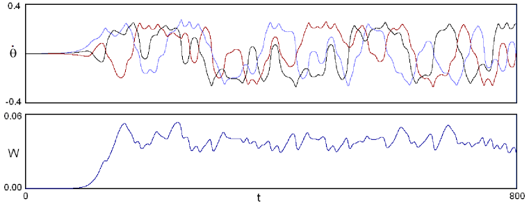
Figure 7: Dependences of the generalized velocities $\dot{\theta}_{1},\,\,\dot{\theta}_{2},\,\,\dot{\theta}_{3}$ and energy $W=\textstyle{1\over 2}(\dot{\theta}_{1}^{2}+\dot{\theta}_{2}^{2}+\dot{\theta}_{3}^{2})$ on time in the transient process of development of chaotic self-oscillations in the mechanical linkage of three self-rotators (16) with $\mu$=0.02, $\nu$=3.

Concerning a number of Lyapunov exponents for the new version of the system, the same arguments as for the previous model are valid; so, four of them are relevant. Figure 9 shows a plot of the Lyapunov exponents versus parameter $\mu$ as computed with the Benettin algorithm. The diagram looks qualitatively similar to that in Fig. 4; so, one can suppose that the hyperbolicity persists despite of the occurrence of energy oscillations in time.

Figure 10 shows the power spectrum of the signal $u(t)=\cos\theta_{1}(t)$ as obtained by processing the time series from numerical simulation of the dynamics on the attractor that demonstrates obvious similarity with Figure 5. Like in the previous case, the spectrum is continuous and looks uniform enough.

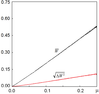
Figure 8: Dependences of the kinetic energy and its standard deviation on the parameter $\mu$ as obtained from numerical integration of equations (16) for the mechanical linkage of three self-rotators at $\nu$=3.

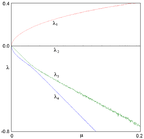
Figure 9: Lyapunov exponents of the linkage of three self-rotators (16) depending on $\mu$ at $\nu$=3.

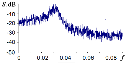
Figure 10: The power spectrum of the signal generated by the system (16) for $\nu$=3 and $\mu$=0.02.

Figure 11 shows histograms of the angles between stable and unstable subspaces in the system (16) obtained numerically for $\nu$=3 with $\mu$=0.02 and 0.13. The distributions do not include angles close to zero, so, the test confirms the hyperbolic nature of the attractor.

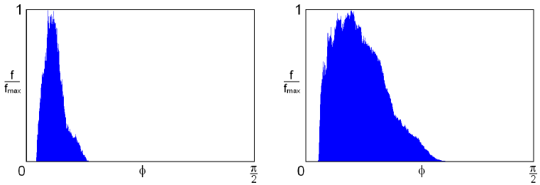
Figure 11: Verification of the criterion of angles in the linkage of three self-rotators (16) at $\mu$=0.02 and $\mu$=0.13 with $\nu$=3.

4 Systems of three rotators with potential
interaction

From systems with mechanical constraints let us move now to a class of systems where the interaction of three constituting components (rotators) is introduced by a potential function depending on the angle variables. We impose a specific form of this function in such a way that the potential minimum is reached on a surface just corresponding to that defined by the equation of mechanical constraint in the previous examples: $U(\theta_{1},\theta_{2},\theta_{3})=\textstyle{1\over 2}(\cos\theta_{1}+\cos\theta_{2}+\cos\theta_{3})^{2}$. Instead of equations (3) we write now

$$\ddot{\theta}_{i}=-\partial U/\partial\theta_{i}+M_{i}=(\cos\theta_{1}+\cos\theta_{2}+\cos\theta_{3})\sin\theta_{1}+M_{i},\,\,i=1,2,3,$$ (17)

where $M_{1,2,3}$ designate external torques supplied to the rotators.

We will consider two options.

In the first case, we assume that the applied torques are defined according to (10) and ensure that the system tends to a level of constant kinetic energy. The set of equations reads

$$\ddot{\theta}_{i}=\nu[\mu-\textstyle{1\over 2}(\dot{\theta}_{1}^{2}+\dot{\theta}_{2}^{2}+\dot{\theta}_{3}^{2})]\dot{\theta}_{i}-(\cos\theta_{1}+\cos\theta_{2}+\cos\theta_{3})\sin\theta_{i},\,\,i=1,2,3.$$ (18)

This system was proposed and particularly studied earlier in Ref. [33].

In the second case, we define the torques by (15), so the system is composed of three self-rotators interacting due to the potential forces, and the equations look as follows:

$$\ddot{\theta}_{i}=\nu(\mu-\textstyle{1\over 2}\dot{\theta}_{i}^{2})\dot{\theta}_{i}-(\cos\theta_{1}+\cos\theta_{2}+\cos\theta_{3})\sin\theta_{i},\,\,i=1,2,3.$$ (19)

Figure 12 illustrates the transient processes in the systems (18) and (19) starting from a state of low energy. In both cases, the result of the transient process is a chaotic self-oscillating mode where the kinetic energy irregularly fluctuates around a mean value. These fluctuations are small in amplitude and have relatively short time scale in the first model. In the second model, the magnitude of the energy undulation is much larger, and the time scale is notably larger: the energy dependence is similar to that for a model with a mechanical constraint in Figure 7.

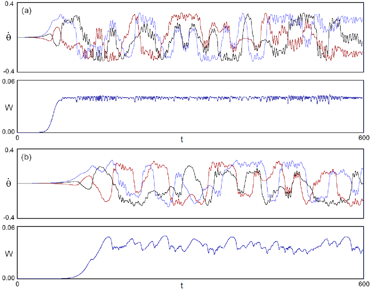
Figure 12: Generalized velocities and kinetic energy versus time in the transient process for system (18) at $\mu$=0.04, $\nu$=3 (a) and in system (19) at $\mu$=0.02, $\nu$=3 (b).

Figure 13 shows trajectories in the configuration space for the systems (18) and (19). For small values of the parameter $\mu$, which correspond to small average energy of the sustained self-oscillatory mode, the orbits are close to the two-dimensional surface defined by the equation $\cos\theta_{1}+\cos\theta_{2}+\cos\theta_{3}=0$, which is consistent with the mechanical constraint imposed in models of two previous sections (diagram (a) and (c)). Hence, we guess that the hyperbolic nature of the dynamics in this domain yet persists. However, one can observe that the trajectory is ”fluffed up” transversally to the surface that reflects the occurrence of fluctuations in the potential energy in the course of the motion in the sustained mode. This effect is still negligible for small $\mu$, but it becomes more pronounced with increase of the parameter, as seen in diagrams (b) and (d). We expect (and this is supported by numerical calculations, see below) that due to this effect the dynamics may change its nature, and ceases to be hyperbolic.

Figure 14 demonstrates the dependence of the average kinetic energy oscillations and standard deviation of the energy on parameter $\mu$ for the models (18) and (19). As is seen, in the second case the energy fluctuations are much more pronounced. This is not surprising, since the models (18) and (19) are modifications of the models (13) and (16) with potential interaction instead of the mechanical constraint, and in the model (13) the energy fluctuations are excluded altogether. In diagram (b), approximately at $\mu\approx$0.18, one observes a sharp change in the dynamical behavior: at larger $\mu$ a regular self-oscillation mode occurs instead of chaos; this mode corresponds to an attractive limit cycle in the phase space.

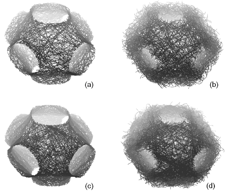
Figure 13: Trajectories in the three-dimensional configuration space on attractors of the system (18) at $\mu$ = 0.04 (a) and $\mu$ = 0.25 (b), and of the system (19) at $\mu$ = 0.02 (c) and $\mu$ = 0.13 (d) for $\nu=3$.

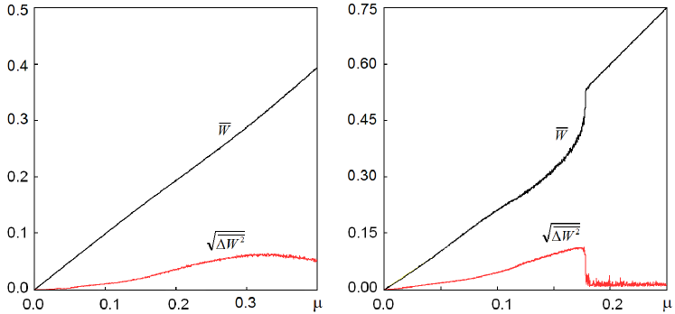
Figure 14: The average kinetic energy of oscillations and its standard deviation depending on parameter $\mu$ for three rotators with potential interaction as obtained numerically for the models (18) (a) and (19) (b) at $\nu$ = 3.

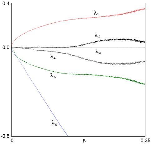
Figure 15: Lyapunov exponents of the system (18) composed of three rotators with interaction potential depending on the parameter $\mu$ at $\nu$=3.

Figures 15 and 16 show graphs of Lyapunov exponents depending on the parameter $\mu$ for the models (18) and (19) calculated with the Benettin algorithm. For these systems, we must take into account all six exponents as there is no reason to exclude any of them from consideration. The presence of a zero exponent is explained by the autonomous nature of the system; it is associated with the perturbation vector tangent to the reference trajectory.

For the system (18), throughout the parameter range shown in the picture, the senior Lyapunov exponent is positive, indicating a chaotic nature of the dynamics. Its parameter dependence is smooth, without drops accompanying the appearance of ”windows of regularity” in many systems with nonhyperbolic attractors. The second exponent in the region of small $\mu$ is close to zero, but then becomes positive. So for $\mu>0.17$ we have two positive exponents; this regime is referred to as hyperchaos [42]. Three exponents remain negative in the whole range, although one of them is close to zero in the region of small $\mu$. Obviously, at small $\mu$, where three exponents are close to zero, we can suggest a possibility of approximate description of the dynamics with replacement of the potential interaction by the mechanical constraint with reduction to the model, discussed in Section 2. Also the possibility of approximation of the exponents $\lambda_{1}$ and $\lambda_{5}$ by $\pm\mbox{const}\cdot\sqrt{W}$, as in the reduced model, is evident from Figure 15.

For the system (19) in the region of small $\mu$ we have one positive, one zero, and four negative Lyapunov exponents. The dependence of the exponents on the parameter is smooth here, without irregularities, which suggests that the hyperbolic chaos persists, as in the reduced model of Section 3. The senior Lyapunov exponent remains positive, and the dynamics is chaotic up to $\mu\approx$0.18. When this point is approached, brokenness arises and progresses in the graph of the senior exponent, which apparently indicates destruction of the hyperbolicity, though no visible drops to zero with formation of regularity windows are distinguished. Then the chaos disappears sharply, and the system manifests transition to the regular mode, where the senior exponent is zero, and the others are negative, which corresponds to the limit cycle.

Figure 17 shows power spectra of the signal $u(t)=\cos\theta_{1}(t)$ generated by the systems (18) and (19) at relatively low values of $\mu$, which correspond presumably to the hyperbolic chaos. They can be compared with that shown in Figure 5 for the model (13), certainly relating to the hyperbolic chaos. The spectra are continuous, which corresponds to the chaotic nature of the dynamics, and evidently are characterized by a relatively high degree of uniformity.

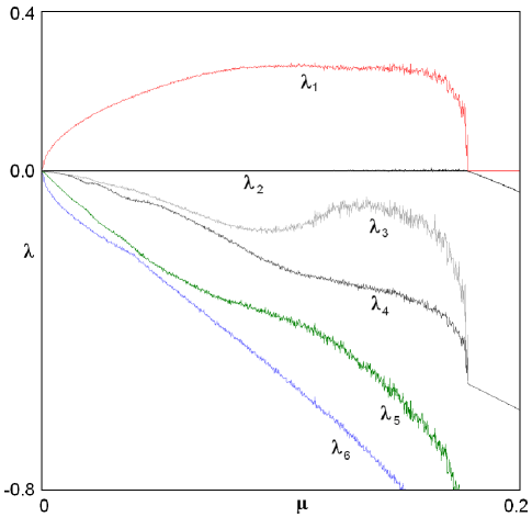
Figure 16: Lyapunov exponents of the system (19) composed of three self-rotators with interaction potential, depending on the supercriticality parameter $\mu$ with $\nu$=3.

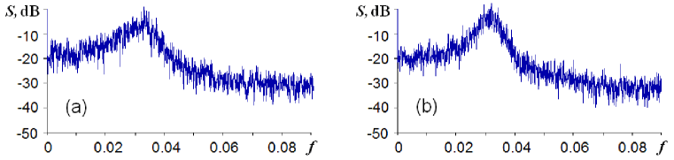
Figure 17: Power spectra of the signal $u(t)=\cos\theta_{1}(t)$ for $\nu$=3 in the system (18) at $\mu$=0.04 (a) and in the system (19) $\mu$=0.02 (b).

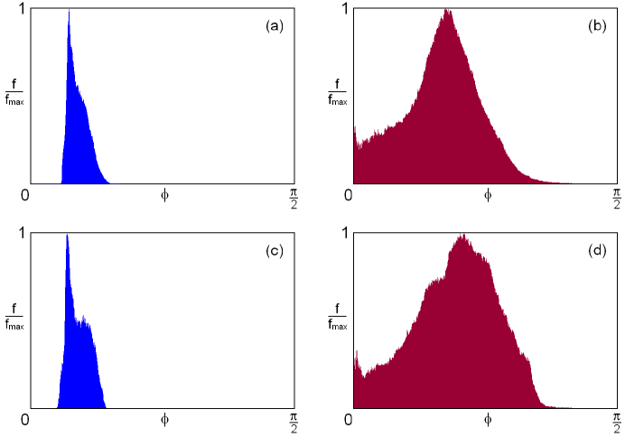
Figure 18: Verification of the criterion of angles for systems of three rotators with potential interaction in the model (18) at $\mu$=0.04 (a) and $\mu$=0.25 (b), and in the model (19) at $\mu$=0.02 (c) and $\mu$=0.13 (d). Histograms (a) and (c) show distributions separated from zero, which indicates the hyperbolic nature of the attractor. Diagrams (b) and (d) show the distributions with positive probability of zero angles indicating occurrences of tangencies of stable and unstable manifolds, which means violation of the hyperbolicity.

Figure 18 shows results of testing the attractors of models (18) and (19) using the criterion of angles. Here the numerically obtained histograms are plotted for the angles between stable and unstable subspaces of perturbation vectors for typical chaotic phase trajectories. At small values of $\mu$ the distributions are disposed at some finite distance from zero, i.e., the test confirms the hyperbolicity. This feature, however, is violated somewhere in the course of increase of $\mu$. Observe that histograms (b) and (d) clearly demonstrate the presence of angles close to zero, which indicates the occurrence of tangencies of stable and unstable manifolds, and, hence, signalizes about non-hyperbolic nature of the attractor. As this phenomenon was not observed in the reduced models of Sections 2 and 3, it is natural to assume that the destruction of hyperbolicity is linked with excursions of phase trajectories relating to the attractor outside a narrow neighborhood of the surface of equal potential in the configuration space.

5 Conclusion

Chaos associated with hyperbolic attractors in dissipative systems and with Anosov dynamics in conservative systems is characterized by roughness, or structural stability as a mathematically rigorously proven attribute. Therefore, devices that generate such chaos should be preferred for any practical applications of chaos as they are robust, i.e., they have low sensitivity to various imperfections, variations of parameters, noise, etc.

A possible productive approach to design systems with hyperbolic chaos starting from some abstract and artificial example of such dynamical behavior consists in its modification to a physically realizable device by variation of functions and parameters involved in the original equations. While the variations are small enough, the hyperbolic nature of the dynamics persists by virtue of the structural stability. However, if we depart further and further from the original system, the hyperbolicity may break up; its preservation must be monitored using some mathematically justified quantitative criteria. One of them is based on analysis of statistical distribution of angles between stable and unstable manifolds of relevant phase trajectories to demonstrate absence of tangencies between these manifolds.

In this article we have discussed several chaotic systems based on the triple linkage hinge mechanism of Thurston, Weeks, Hunt, and MacKay. The original system is composed of three elements able to rotate about fixed axles with mechanical constraint imposed with some hinges and rods. We modify the model and introduce activity and dissipation by adding appropriate terms in the equations to get examples of systems with hyperbolic chaotic attractors. In one version, these additional terms are chosen to provide a tendency to approach a constant level of kinetic energy. In another more pragmatic setup, each of the three basic elements is represented by a self-rotator that is a subsystem, which, being isolated, tends to rotate in one or other direction with constant angular velocity.

Results of numerical simulations are presented, and characteristics of the attractors (Lyapunov exponents, power spectra) are discussed. Robust chaos is observed in the models under study in wide ranges, being not destroyed under variation of parameters. The calculations have been performed for verification of the criterion of angles, and confirmation of the hyperbolic nature of attractors is provided in the considered models, at least, for self-oscillatory modes of small supercriticality.

An alternative approach to a more rigorous substantiation of hyperbolicity may be based on computer verification of the so-called Alekseev cone criterion [43, 4, 44, 13]. In Ref. [30] the authors consider the application of the cone criterion to justification of Anosov dynamics for linkages where the curvature is not globally negative (some areas of positive curvature are present). One more approach consists in analyzing invariant measure; on hyperbolic attractors it must correspond to the concept of Sinai – Ruelle – Bowen measures [3, 4, 13].

Besides the models with mechanical constraints, we have suggested and considered systems manifesting analogous dynamical behavior, where interaction of the rotators is provided by potential forces. In principle, it opens up a prospect to go away from mechanics and implement systems of a different nature, e.g., electronic devices operating as generators of robust chaos. They will manifest hyperbolic dynamics, roughly uniform in continuous time, in contrast to previously proposed systems [13, 14]; apparently, it will improve essentially the spectral properties of the generated chaotic signals.

This work was supported by RNF grant No 15-12-20035.

References

- [1] Smale, S., Differentiable Dynamical Systems, Bull. Amer. Math. Soc. (NS), 1967, vol. 73, pp. 747-817.
- [2] Shilnikov, L., Mathematical Problems of Nonlinear Dynamics: A Tutorial, Internat. J. Bifur. Chaos Appl. Sci. Engrg., 1997, vol. 7, no. 9, pp. 1953-2001.
- [3] Dynamical Systems 9: Dynamical Systems with Hyperbolic Behaviour, D.V.Anosov (Ed.), Encyclopaedia Math. Sci., vol. 9, Berlin: Springer, 1995.
- [4] Katok, A. and Hasselblatt, B., Introduction to the Modern Theory of Dynamical Systems, Cambridge: Cambridge University Press, 1996.
- [5] Afraimovich, V. and Hsu, S.-B., Lectures on Chaotic Dynamical Systems, AMS/IP Studies in Advanced Mathematics, vol. 28, Providence, RI: Amer. Math. Soc., Somerville, MA: International Press, 2003.
- [6] Pesin, Ya.B., Lectures on partial hyperbolicity and stable ergodicity. Zurich lectures in advanced mathematics, European Mathematical Society, 2004.
- [7] Bonatti, C., Diaz, L.J., Viana, M., Dynamics Beyond Uniform Hyperbolicity. A Global Geometric and Probobalistic Perspective. Encyclopedia of Mathematical Sciences, vol.102, Berlin, Heidelberg, New-York: Springer, 2005.
- [8] Kuznetsov, S.P., Example of a Physical System with a Hyperbolic Attractor of the Smale–Williams Type, Phys. Rev. Lett., 2005, vol. 95, 144101.
- [9] Kuznetsov, S.P. and Seleznev, E.P., Strange Attractor of Smale–Williams Type in the Chaotic Dynamics of a Physical System, Zh. Eksper. Teoret. Fiz., 2006, vol. 129, no. 2, pp. 400-412 [J. Exp. Theor. Phys., 2006, vol. 102, no. 2, pp. 355-364].
- [10] Isaeva, O.B., Jalnine, A.Y., Kuznetsov, S.P., Arnold’s cat map dynamics in a system of coupled nonautonomous van der Pol oscillators, Physical Review E, 2006, vol. 74, no 4, p. 046207.
- [11] Kuznetsov, S.P. and Pikovsky, A. Autonomous Coupled Oscillators with Hyperbolic Strange Attractors, Physica D, 2007, vol. 232, pp. 87-102.
- [12] Kuznetsov, S.P., Example of Blue Sky Catastrophe Accompanied by a Birth of Smale–Williams Attractor, Regular and Chaotic Dynamics, 2010, vol. 15, nos. 2-3, pp. 348-353.
- [13] Kuznetsov, S.P., Hyperbolic Chaos: A Physicist’s View, Berlin: Springer, 2012.
- [14] Kuznetsov, S.P., Dynamical Chaos and Uniformly Hyperbolic Attractors: From Mathematics to Physics, Phys. Uspekhi, 2011, vol. 54, no. 2, pp. 119-144; see also: Uspekhi Fiz. Nauk, 2011, vol. 181, pp. 121-149.
- [15] Kuznetsov, S.P., Plykin type attractor in electronic device simulated in MULTISIM, Chaos: An Interdiskiplinary Journal of Nonlinear Science, 2011, vol. 21, no 4, p. 043105.
- [16] Isaeva, O.B., Kuznetsov, S.P., and Mosekilde, E., Hyperbolic chaotic attractor in amplitude dynamics of coupled self-oscillators with periodic parameter modulation, Physical Review E., 2011, vol. 84, no. 1, p. 016228.
- [17] Isaeva, O.B., Kuznetsov, A.S., Kuznetsov, S.P., Hyperbolic chaos in parametric oscillations of a string, Rus. J. Nonlin. Dyn., 2013, vol. 9, no. 1, pp. 3-10
- [18] Kuznetsov S.P., Kuznetsov A.S., Kruglov V.P., Hyperbolic chaos in systems with parametrically excited patterns of standing waves, Rus. J. Nonlin. Dyn., 2014, vol. 10, no. 3, pp. 265-277. (Russian.)
- [19] Jalnine, A.Y., Hyperbolic and non-hyperbolic chaos in a pair of coupled alternately excited FitzHugh–Nagumo systems, Communications in Nonlinear Science and Numerical Simulation, 2015, vol. 23, no. 1, pp. 202-208.
- [20] Kuznetsov, S.P., Some mechanical systems manifesting robust chaos, Nonlinear Dynamics and Mobile Robotics, 2013, vol. 1, no. 1, pp. 3-22.
- [21] Borisov, A.V., Kazakov, A.O., and Kuznetsov, S.P., Nonlinear dynamics of the rattleback: a nonholonomic model, Physics-Uspekhi, 2014, vol. 57, no. 5, pp. 453-460; see also: Uspekhi Fiz. Nauk, 2014, vol. 184, pp. 493-500.
- [22] Kuznetsov, S.P., Plate falling in a fluid: Regular and chaotic dynamics of finite-dimensional models, Regular and Chaotic Dynamics, 2015, vol. 20, no. 3, pp. 345-382.
- [23] Borisov, A.V., Mamaev, I.S., On the motion of a heavy rigid body in an ideal fluid with circulation, Chaos: An Interdiskiplinary Journal of Nonlinear Science, 2006, vol. 16, no. 1, p. 013118.
- [24] Borisov, A.V., Jalnine, A.Y., Kuznetsov, S.P., Sataev, I.R., and Sedova, J.V., Dynamical phenomena occurring due to phase volume compression in nonholonomic model of the rattleback, Regular and Chaotic Dynamics, 2012, vol. 17, no. 6, pp. 512-532.
- [25] Thurston, W.P. and Weeks, J.R., The mathematics of three-dimensional manifolds, Sci. Am., 1984, vol. 251, pp. 94-106.
- [26] Kozlov, V.V., Topological obstacles to the integrability of natural mechanical systems, Soviet Math. Dokl., 1980, vol. 20, pp. 1413-1415.
- [27] Anosov, D.V., Geodesic flows on closed Riemannian manifolds of negative curvature, Trudy Mat. Inst. Steklov, 1967, vol. 90, pp. 3-210.
- [28] Balazs, N.L. and Voros, A., Chaos on the pseudosphere, Physics Reports, 1986, vol. 143, no. 3, pp. 109-240.
- [29] Hunt, T.J. and MacKay, R.S., Anosov Parameter Values for the Triple Linkage and a Physical System with a Uniformly Chaotic Attractor, Nonlinearity, 2003, vol. 16, pp. 1499-1510.
- [30] Magalhães, M. L. S. and Pollicott, M., Geometry and dynamics of planar linkages, Communications in Mathematical Physics, 2013, vol. 317, no. 3, pp. 615-634.
- [31] Kourganoff, M., Anosov geodesic flows, billiards and linkages, arXiv:1503.04305, 2015, pp. 1-27.
- [32] Kozlov, V.V., Closed orbits and chaotic dynamics of a charged particle in a periodic electromagnetic field, Regular and Chaotic Dynamics, 1997, vol. 2, no. 1, pp. 3-12.
- [33] Kuznetsov, S.P., Chaos in the system of three coupled rotators: from Anosov dynamics to hyperbolic attractor, Proceedings of Saratov University – New series. Series Physics, 2015, vol. 15, no. 2, pp. 5-17. (Russian.)
- [34] Lai, Y.-C., Grebogi, C., Yorke, J. A., Kan, I., How often are chaotic saddles nonhyperbolic? Nonlinearity, 1993, vol. 6, pp. 779-798.
- [35] Anishchenko, V.S., Kopeikin, A.S., Kurths, J., Vadivasova, T.E., Strelkova G.I., Studying hyperbolicity in chaotic systems, Physics Letters A, 2000, vol. 270, pp. 301-307.
- [36] Ginelli, F., Poggi, P., Turchi, A., Chaté, H., Livi, R., Politi, A., Characterizing Dynamics with Covariant Lyapunov Vectors, Phys. Rev. Lett., 2007, vol. 99, p. 130601.
- [37] Kuptsov, P.V., Fast numerical test of hyperbolic chaos, Physical Review E, 2012, vol. 85, no 1, p. 015203.
- [38] Gantmakher, F.R., Lectures in analytical mechanics, Moscow: Mir Publishers, 1970.
- [39] Goldstein, H., Poole, C.P., Safko, J.L., Classical Mechanics (3rd ed.). Addison-Wesley, 2001.
- [40] Benettin, G., Galgani, L., Giorgilli, A., and Strelcyn, J.-M., Lyapunov Characteristic Exponents for Smooth Dynamical Systems and for Hamiltonian Systems: A Method for Computing All of Them, Meccanica, 1980, vol. 15, pp. 9-30.
- [41] Jenkins, G.M. and Watts, D.G.: Spectral analysis and its application. San Francisco: Holden-Day, Inc., 1968.
- [42] Rössler, O. E., An equation for hyperchaos, Physics Letters A, 1979, vol. 71, no. 2, pp. 155-157.
- [43] Sinai, Y.G., Stochasticity of dynamical systems. In: Gaponov-Grekhov, A.V. (ed.), Nonlinear Waves, Moscow: Nauka, 1979, pp.192-212. (Russian.)
- [44] Kuznetsov, S.P. and Sataev, I.R., Hyperbolic attractor in a system of coupled non-autonomous van der Pol oscillators: Numerical test for expanding and contracting cones, Physics Letters A, 2007, 365, nos. 1-2, pp. 97-104.