Coupling Importance Sampling and Multilevel Monte Carlo using Sample Average Approximation

Abstract

In this work, we propose a smart idea to couple importance sampling and Multilevel Monte Carlo (MLMC). We advocate a per level approach with as many importance sampling parameters as the number of levels, which enables us to handle the different levels independently. The search for parameters is carried out using sample average approximation, which basically consists in applying deterministic optimisation techniques to a Monte Carlo approximation rather than resorting to stochastic approximation. Our innovative estimator leads to a robust and efficient procedure reducing both the discretization error (the bias) and the variance for a given computational effort. In the setting of discretized diffusions, we prove that our estimator satisfies a strong law of large numbers and a central limit theorem with optimal limiting variance, in the sense that this is the variance achieved by the best importance sampling measure (among the class of changes we consider), which is however non tractable. Finally, we illustrate the efficiency of our method on several numerical challenges coming from quantitative finance and show that it outperforms the standard MLMC estimator.

AMS 2000 Mathematics Subject Classification. 60F05, 62F12, 65C05, 60H35.

Key Words and Phrases. Sample average approximation; multilevel Monte Carlo; variance reduction; uniform strong large law of numbers; central limit theorem; importance Sampling.

1 Introduction

Expectations involving a stochastic process are often computed using a Monte Carlo method combined with a discretization scheme. For instance, computing a hedging portfolio in finance uses these tools. Generally, the asset price is modeled by a diffusion process $(X_{t})_{0\leq t\leq T}$, defined as the solution of a stochastic differential equation (SDE)

$$dX_{t}=b(X_{t})dt+\sigma(X_{t})dW_{t},\quad X_{0}=x\in\mathbb{R}^{d}$$ (1.1)

where $b:{\mathbb{R}}^{d}\to{\mathbb{R}}^{d}$, $\sigma:{\mathbb{R}}^{d}\to{\cal M}_{d\times q}$ and $W$ is a Brownian motion with values in ${\mathbb{R}}^{q}$ defined on some given probability space $(\Omega,(\mathcal{F}_{t})_{0\leq t\leq T},{\mathbb{P}})$ with finite time horizon $T>0$. The process $X$ hardly ever has an explicit solution, which implies that its simulation requires the use of a discretization scheme. For $n\in{\mathbb{N}}^{*}$, consider the continuous time Euler approximation $X^{n}$ with time step $\delta=T/n$ given by

$$dX^{n}_{t}=b(X^{n}_{\eta_{n}(t)})dt+\sigma(X^{n}_{\eta_{n}(t)})dW_{t},\quad\eta_{n}(t)=\lfloor t/\delta\rfloor\delta.$$

This work aims at combining importance sampling with different discretization methods: first, we study the use of importance sampling for the standard case of Euler Monte Carlo and then we apply it to MLMC. Many different changes of measure can be used to implement importance sampling. When working with Lévy processes, it is common to use the Esscher transform to introduce a new family of measures. For Brownian driven SDEs, the Esscher transform actually corresponds to a Gaussian change of measure in the spirit of the Girsanov theorem. Following the ideas of Arouna [1], we consider a parametric family of stochastic processes $(X_{t}({\theta}))_{0\leq t\leq T}$, with $\theta\in{\mathbb{R}}^{q}$, driven by a Brownian motion with linear drift

$$dX_{t}(\theta)=\left(b(X_{t}(\theta))+\sigma(X_{t}(\theta))\theta\right)dt+\sigma(X_{t}(\theta))dW_{t}.$$

We also define the continuous time Euler approximation $X^{n}(\theta)$ of the process $X(\theta)$. From Girsanov’s Theorem, the process $(B^{\theta}_{t}\stackrel{{\scriptstyle\Delta}}{{=}}W_{t}+\theta t)_{t\leq T}$ is a Brownian motion under the new probability measure ${\mathbb{P}}_{\theta}$ equivalent to ${\mathbb{P}}$ and such that

$$\frac{d{\mathbb{P}}_{\theta}}{d{\mathbb{P}}}_{|{\cal F}_{t}}=\exp\left(-\theta\cdot W_{t}-\frac{1}{2}|\theta|^{2}t\right)\stackrel{{\scriptstyle\Delta}}{{=}}{\cal E}^{-}(W,\theta).$$

Therefore,

$${\mathbb{E}}_{{\mathbb{P}}}[\psi(X_{T})]={\mathbb{E}}_{{\mathbb{P}}_{\theta}}[\psi(X_{T}(\theta))]={\mathbb{E}}_{{\mathbb{P}}}\left[\psi(X_{T}(\theta)){\cal E}^{-}(W,\theta)\right].$$ (1.2)

This equality still holds when replacing $X$ (resp. $X(\theta)$) by its Euler scheme $X^{n}$ (resp. $X^{n}(\theta)$). The l.h.s. and r.h.s. expectations are both computed under the original probability measure. In the following, we will always use the measure ${\mathbb{P}}$ and therefore we will not write it anymore. The idea of importance sampling Monte Carlo is to use the r.h.s of (1.2) to build a Monte Carlo estimator of ${\mathbb{E}}[\psi(X_{T})]$ using $X^{n}(\theta)$ with $\theta$ given by

$$\theta^{\star}=\operatorname*{\arg\!\min}_{\theta\in{\mathbb{R}}^{q}}\mathrm{Var}\left(\psi(X_{T}(\theta)){\cal E}^{-}(W,\theta)\right).$$

Importance sampling for Euler Monte Carlo is studied in Section 2: first, we investigate how to approximate $\theta^{\star}$ in practice and second we prove that the Monte Carlo estimator combined with this approximation of $\theta^{\star}$ satisfies a strong law of large numbers and a central limit theorem when both $n$ and the number of samples go to infinity. This result extends the limit theorems obtained in [23], in which the authors investigated the case of a fixed number of discretization steps $n$. The error induced by using ${\mathbb{E}}[\psi(X^{n}_{T}(\theta))]$ instead of ${\mathbb{E}}[\psi(X_{T}(\theta))]$ is called the discretization error and is responsible for the bias of the Euler Monte Carlo estimator, while the Monte Carlo approximation only impacts the variance. The two errors are balanced when the number of samples $N$ of the Monte Carlo method is proportional to $n^{2}$, which leads to an overall complexity of order $n^{3}$. In order to reduce the bias for a given computational effort, Kebaier [24] proposed to use the Statistical Romberg method, which combines discretization schemes on two nested time grids. This method was generalized by Giles [13] who proposed to use a multilevel Monte Carlo algorithm following the line of Heinrich’s multilevel method for parametric integration [19].

Let $m,L\in{\mathbb{N}}$ with $m\geq 2$ and $L>0$, the idea of the multilevel method is to write the expectation on the finest time grid as a telescopic sum involving all the other grids (referred to as levels)

$${\mathbb{E}}[\psi(X_{T}^{m^{L}})]={\mathbb{E}}[\psi(X_{T}^{m^{0}})]+\sum_{\ell=1}^{L}{\mathbb{E}}[\psi(X_{T}^{m^{\ell}})-\psi(X_{T}^{m^{\ell-1}})]$$ (1.3)

and then to approximate each expectation by a Monte Carlo method with a well chosen number of samples to balance the errors between the different terms. We refer the reader to the extensive literature on MLMC for more details, see e.g. [3, 9, 10, 11, 14, 16, 15, 18, 20, 27]. For a fixed computational budget, the use of multilevel techniques clearly reduces the bias, but in many situations the high variance also brings in a significant inaccuracy, which naturally leads to trying to couple MLMC with variance reduction techniques.

In this work, we focus on coupling importance sampling with MLMC. In [5] and [17], the authors choose to apply MLMC to the right hand side of (1.2) coming up with

$$\begin{split}{\mathbb{E}}[\psi(X_{T}^{m^{L}})]&={\mathbb{E}}\left[\psi(X_{T}^{m^{0}}(\lambda)){\cal E}^{-}(W,\lambda)\right]\\ &\quad+\sum_{\ell=1}^{L}{\mathbb{E}}\left[(\psi(X_{T}^{m^{\ell}}(\lambda))-\psi(X_{T}^{m^{\ell-1}}(\lambda))){\cal E}^{-}(W,\lambda)\right].\end{split}$$ (1.4)

This approach mixes all the levels through the optimization of the parameter $\lambda$ and breaks the independence between the levels of the multilevel approach, which nonetheless made it so popular and easy to implement.

Instead of using (1.4), we would rather apply importance sampling to each expectation in the telescopic sum of (1.3) to obtain for $\lambda_{1},\dots,\lambda_{L}\in{\mathbb{R}}^{q}$

$${\mathbb{E}}[\psi(X_{T}^{m^{L}})] ={\mathbb{E}}\left[\psi(X_{T}^{m^{0}}(\lambda_{0})){\cal E}^{-}(W,\lambda_{0})\right]$$

$$\quad+\sum_{\ell=1}^{L}{\mathbb{E}}\left[(\psi(X_{T}^{m^{\ell}}(\lambda_{\ell}))-\psi(X_{T}^{m^{\ell-1}}(\lambda_{\ell}))){\cal E}^{-}(W,\lambda_{\ell})\right].$$

Our importance sampling multilevel estimator is obtained by applying a Monte Carlo method to each of the levels $\ell$ with $N_{\ell}$ samples

$$Q_{L}(\lambda_{0},\dots,\lambda_{L}) =\frac{1}{N_{0}}\sum_{k=1}^{N_{0}}\psi({\tilde{X}}^{m^{0}}_{T,0,k}(\lambda_{0})){\cal E}^{-}(\tilde{W}_{0,k},\lambda_{0})$$

$$\qquad+\sum_{\ell=1}^{L}\frac{1}{N_{\ell}}\sum_{k=1}^{N_{\ell}}\left(\psi({\tilde{X}}^{m^{\ell}}_{T,\ell,k}(\lambda_{\ell}))-\psi({\tilde{X}}^{m^{\ell-1}}_{T,\ell,k}(\lambda_{\ell}))\right){\cal E}^{-}(\tilde{W}_{\ell,k},\lambda_{\ell})$$ (1.5)

The samples used in the different levels are independent and within each level they are i.i.d. For any $\ell\geq 0$, the variables ${\tilde{X}}^{m^{\ell}}_{T,\ell,k}(\lambda_{\ell})$ (resp. ${\tilde{X}}^{m^{\ell-1}}_{T,\ell,k}(\lambda_{\ell})$ when $\ell>0$) are the terminal values of the Euler schemes of $X(\lambda_{\ell})$ with $m^{\ell}$ (resp. $m^{\ell-1}$) time steps built using the same Brownian path $\tilde{W}_{\ell,k}$. The variance of the importance sampling MLMC estimator is given by

$$\mathrm{Var}[Q_{L}]=N_{0}^{-1}\sigma_{0}(\lambda_{0})^{2}+\sum_{\ell=1}^{L}N^{-1}_{\ell}\frac{(m-1)T}{m^{\ell}}\sigma_{\ell}^{2}(\lambda_{\ell})$$

where

$$\sigma_{0}^{2}(\lambda_{0}) \stackrel{{\scriptstyle\Delta}}{{=}}\mathrm{Var}[\psi(X^{m^{0}}_{T}(\lambda_{0})){\cal E}^{-}(W,\lambda_{0})]$$

$$\sigma_{\ell}^{2}(\lambda_{\ell}) \stackrel{{\scriptstyle\Delta}}{{=}}\frac{m^{\ell}}{(m-1)T}\mathrm{Var}\left[\left(\psi(X^{m^{\ell}}_{T}(\lambda_{\ell}))-\psi(X^{m^{\ell-1}}_{T}(\lambda_{\ell}))\right){\cal E}^{-}(W,\lambda_{\ell})\right].$$

By allowing for one importance sampling parameter $\lambda_{\ell}$ per level, our approach has many advantages over [5, 17]. First, the computations within the different levels remain independent. Second, the variance of each level $\ell$ only depends on $\lambda_{\ell}$, which reduces the global minimization problem to several smaller minimization problems. Third, we actually minimize the real variance of the estimator and not its asymptotic value and more importantly it can be implemented without knowing $\nabla\psi$, which however appears in the central limit theorem for MLMC. The new idea of using one importance sampling parameter per level was later taken up in [6] but coupled with stochastic approximation to build adaptive estimators.

Actually, minimizing $\lambda\longmapsto\sigma_{\ell}^{2}(\lambda)$ can be achieved by using the randomly truncated Robbins Monro algorithm proposed by Chen et al. [7, 8] and later investigated in the context of importance sampling by Lapeyre and Lelong [25] and Lelong [26]. The numerical stability of these stochastic algorithms strongly depends on the choice of the descent step — often referred to as the gain sequence — which proves to be highly sensitive in practice. To overcome this difficulty, Jourdain and Lelong [23] proposed to apply deterministic optimization techniques to sample average estimators to search for the optimal parameter. Following their methodology, we define $\sigma_{\ell,N_{\ell}^{\prime}}^{2}$ as the sample average approximation of $\sigma_{\ell}^{2}$ with $N_{\ell}^{\prime}$ samples using the standard empirical Monte Carlo estimator of the variance. We assume that the samples used in $\sigma_{\ell,N_{\ell}^{\prime}}^{2}$ are independent of those used in $Q_{L}$. We refer to Section 3 for more details on how to choose the samples in the different approximations. Now, we sketch the algorithm corresponding to our method.

1 for $\ell=0:L$ do

       Sample the random function $\lambda\longmapsto\sigma_{\ell,N_{\ell}^{\prime}}(\lambda)$.

        // $\sigma_{\ell,N_{\ell}^{\prime}}^{2}$ is the sample average approximation of $\sigma_{\ell}^{2}$, see Section 3.1

2       Compute $\hat{\lambda}_{\ell}=\operatorname*{\arg\!\min}\sigma_{\ell,N_{\ell}^{\prime}}^{2}(\lambda)$ using Newton–Raphson’s algorithm.

3       Independently of $\sigma_{\ell,N_{\ell}^{\prime}}^{2}$, sample the level $\ell$ of (1) using $\hat{\lambda}_{\ell}$.

4      

5 end for

Sum all the levels to obtain

$$Q_{L}(\hat{\lambda}_{0},\dots,\hat{\lambda}_{L}) =\frac{1}{N_{0}}\sum_{k=1}^{N_{0}}\psi({\tilde{X}}^{m^{0}}_{T,0,k}(\hat{\lambda}_{0})){\cal E}^{-}(\tilde{W}_{0,k},\hat{\lambda}_{0})$$

$$\qquad+\sum_{\ell=1}^{L}\frac{1}{N_{\ell}}\sum_{k=1}^{N_{\ell}}\left(\psi({\tilde{X}}^{m^{\ell}}_{T,\ell,k}(\hat{\lambda}_{\ell}))-\psi({\tilde{X}}^{m^{\ell-1}}_{T,\ell,k}(\hat{\lambda}_{\ell}))\right){\cal E}^{-}(\tilde{W}_{\ell,k},\hat{\lambda}_{\ell}).$$

Algorithm 1.1 Multilevel Importance Sampling (MLIS)

First, we investigate in Section 2 the standard Euler Monte Carlo method coupled with importance sampling. Then, in Section 3, we study the importance sampling framework with MLMC. We prove that $Q_{L}(\hat{\lambda}_{0},\dots,\hat{\lambda}_{L})$ satisfies a strong law of large numbers and a central limit theorem. Our MLIS estimator achieves the smallest possible variance within the family of MLMC estimators approximating ${\mathbb{E}}[\psi(X_{T})]$ using the class of processes $(X(\lambda))_{\lambda\in{\mathbb{R}}^{q}}$. Note that this is also the limiting variance obtained in [5] for the MLMC estimator built on (1.4) with the best possible parameter $\lambda\in{\mathbb{R}}^{q}$. The main difficulty in proving these results is the uniform control of the triangular arrays involved in the adaptive multilevel estimator. To overcome this issue, we prove in Section 4 new limit theorems for doubly indexed sequences of random variables in a general setting (see Propositions 4.1 and 4.3). In section 5, we illustrate the efficiency of MLIS on challenging problems coming from quantitative finance and show that it outperforms the standard MLMC estimator.

2 Importance sampling with Euler Monte Carlo

2.1 Notation and general assumptions

• For a vector $x\in{\mathbb{R}}^{q}$, $\left|x\right|$ denotes the Euclidean norm of $x$.

• The superscript ^∗ denotes the transpose operator.

• For a matrix $A\in{\cal M}_{d\times q}$, $\left|M\right|$ denotes the Frobenius norm of $A$ defined by $\sqrt{\mathrm{Tr}(A^{*}A)}$, which corresponds to the Euclidean norm on ${\mathbb{R}}^{d\times q}$.

• For $q\in{\mathbb{N}}^{*}$, $I_{q}$ denotes the identity matrix with size $q\times q$.

• For $\alpha>0$, we define the set of functions

  $${\cal H}_{\alpha}=\Big{\{} \psi:{\mathbb{R}}^{d}\rightarrow{\mathbb{R}}\mbox{ s.t. }\exists c>0,\beta\geq 1,\;\forall x\in{\mathbb{R}}^{d},\;|\psi(x)|\leq c(1+|x|^{\beta})$$

  $$\quad\mbox{and }\forall x,y\in{\mathbb{R}}^{d},\;|\psi(x)-\psi(y)|\leq c(1+(|x|^{\beta}\wedge|y|^{\beta}))|x-y|^{\alpha}\Big{\}}$$ (2.1)

• For a sequence of random variables $(X_{n})_{n}$, “$X_{n}\Longrightarrow X$” means that $(X_{n})_{n}$ converges in distribution to $X$.

Here, we gather several standard assumptions required to ensure the convergence of the Euler scheme.

• 1. The functions $b$ and $\sigma$ are Lipschitz

     $$\quad\forall x,y\in\mathbb{R}^{d},\quad|b(x)-b(y)|+\left|\sigma(x)-\sigma(y)\right|\leq C_{b,\sigma}|x-y|, \mathcal{H}_{b,\sigma}$$ ()

     for some real number $C_{b,\sigma}>0$.

  2. $\forall p\geq 1,\;X,X^{n}\in L^{p}$ and there exists $K_{p}(T)>0$ s.t.

     $${\mathbb{E}}\left[{\sup_{0\leq t\leq T}}\left|X_{t}-{X}^{n}_{t}\right|^{p}\right]\leq\frac{K_{p}(T)}{n^{p/2}}.$$

  3. There exist $\gamma\in[1/2,1]$ and $C_{\psi}(T,\gamma)>0$ s.t.

     $$n^{\gamma}({\mathbb{E}}\psi(X^{n}_{T})-{\mathbb{E}}\psi(X_{T}))\rightarrow C_{\psi}(T,\gamma). {\cal H}_{\gamma}$$ ()

• The function $\psi$ satisfies

  $${\mathbb{P}}(\psi(X_{T})\neq 0)>0\quad\text{and}\quad\forall\,\theta\in{\mathbb{R}}^{q},\;{\mathbb{E}}\left[\psi(X_{T})^{2}\mathrm{e}^{-\theta\cdot W_{T}}\right]<\infty.$$ (2.2)

2.2 General framework

In this section, we investigate the case of an Euler Monte Carlo approach. We consider the importance sampling representation of ${\mathbb{E}}[\psi(X_{T})]$ given by

$${\mathbb{E}}[\psi(X_{T}(\theta)){\cal E}^{-}(W,\theta)].$$

The optimal value for $\theta$ is given by

$$\theta^{\star}=\operatorname*{\arg\!\min}_{\theta\in{\mathbb{R}}^{q}}\quad\mbox{ with }\quad v(\theta)\stackrel{{\scriptstyle\Delta}}{{=}}{\mathbb{E}}[(\psi(X_{T}(\theta)){\cal E}^{-}(W,\theta))^{2}].$$

By using (1.2), we can rewrite $v$ as

$$v(\theta)={\mathbb{E}}[\psi(X_{T})^{2}{\cal E}^{+}(W,\theta)]\quad\mbox{ with }\quad{\cal E}^{+}(W,\theta)\stackrel{{\scriptstyle\Delta}}{{=}}\mathrm{e}^{-W_{T}\cdot\theta+\frac{\left|\theta\right|}{2}}.$$

From a practical point of view, the quantity $v(\theta)$ is not explicit so we use the Euler scheme to discretize $X(\theta)$ and approximate $\theta^{\star}$ by

$$\theta_{n}\stackrel{{\scriptstyle\Delta}}{{=}}\operatorname*{\arg\!\min}_{\theta\in{\mathbb{R}}^{q}}v_{n}(\theta)\quad\mbox{ with }\quad v_{n}(\theta)\stackrel{{\scriptstyle\Delta}}{{=}}{\mathbb{E}}\left[\psi(X_{T}^{n})^{2}{\cal E}(W,\theta)\right].$$ (2.3)

Since the expectation is usually not tractable, we replace it by its sample average approximation and define

$$\theta_{n,N}\stackrel{{\scriptstyle\Delta}}{{=}}\operatorname*{\arg\!\min}_{\theta\in{\mathbb{R}}^{q}}v_{n,N}(\theta)\quad\mbox{ with }\quad v_{n,N}(\theta)\stackrel{{\scriptstyle\Delta}}{{=}}\frac{1}{N}\sum_{i=1}^{N}\left(\psi(X^{n}_{T,i})^{2}{\cal E}(W_{i},\theta)\right),$$ (2.4)

where $(X^{n}_{T,i},W_{T,i})_{1\leq i\leq N}$ are i.i.d. samples with the law of $(X^{n}_{T},W_{T})$. The existence and uniqueness of $\theta^{\star}$, $\theta_{n}$ and $\theta_{n,N}$ are ensured by the following lemma whose proof can easily be adapted from [23, Lemma 1.1].

Lemma 2.1.

Under Condition (${\mathcal{H}}$-2), the functions $v$, $v_{n}$ and $v_{n,N}$ are infinitely continuously differentiable for all $n,N$ and the derivatives are obtained by exchanging expectation and differentiation. Moreover, the functions $v$ and $v_{n}$ are strongly convex and so is $v_{n,N}$ for any $N$ such that $v_{n,N}$ is not identically zero.

2.3 Convergence of the optimal importance sampling parameter

Theorem 2.2.

Suppose $\sigma$ and $b$ satisfy ($\mathcal{H}_{b,\sigma}$). Let $\psi$ satisfy Condition (${\mathcal{H}}$-2) and belong to ${\cal H}_{\alpha}$ for some $\alpha>0$. Then, $\theta_{n}\to\theta^{\star}$ a.s. when $n\to+\infty$.

By Hölder’s inequality, for any function $\psi\in{\cal H}_{\alpha}$, (${\mathcal{H}}$-2) implies that $\sup_{n}{\mathbb{E}}[\psi(X^{n}_{T})^{2}\mathrm{e}^{-\theta\cdot W_{T}}]<+\infty$. Hence, the proof of the theorem ensues from [5, Theorem 2.2].

In the following, we let $N$ depend on $n$ so that $N\stackrel{{\scriptstyle\Delta}}{{=}}N_{n}$ tends to infinity with $n$.

Proposition 2.3.

Assume that Assumption ($\mathcal{H}_{b,\sigma}$) holds and that $\psi\in{\cal H}_{\alpha}$ for some $\alpha>0$. Then, for all $K>0$, a.s. when $n\to\infty$

$$\sup_{|\theta|\leq K}|v_{n,N_{n}}(\theta)-v(\theta)|\to 0;\;\sup_{|\theta|\leq K}|\nabla v_{n,N_{n}}(\theta)-\nabla v(\theta)|\to 0.$$

Proof.

The proof of the two results are very similar, we omit the second one and concentrate on the uniform convergence for $v_{n,N_{n}}$. To do so, we will apply Proposition 4.3. Now, we check Assumptions (${\mathcal{H}}$-4), (${\mathcal{H}}$-5), (${\mathcal{H}}$-6). At first, note that under Assumption ($\mathcal{H}_{b,\sigma}$), we have the almost sure convergence of $X^{n}_{T}$ towards $X_{T}$. As $\psi\in\mathcal{H}_{\alpha}$, it follows from Property (${\mathcal{H}}$-1)-ii that for all $a>1$, $\sup_{n\in{\mathbb{N}}}{\mathbb{E}}\left[\left|\psi(X^{n}_{T})^{2}e^{-\theta\cdot W_{T}+\frac{1}{2}|\theta|^{2}T}\right|^{a}\right]<\infty$. Note that for every fixed $n$, the sequence $\left(\psi(X^{n}_{T,i})^{2}e^{-\theta\cdot W_{T,i}+\frac{1}{2}|\theta|^{2}T}\right)_{i}$ is i.i.d. Then, we deduce that for all $m\in{\mathbb{N}}^{*}$

$$\lim_{n\rightarrow\infty}{\mathbb{E}}\left[v_{n,m}(\theta)\right]={\mathbb{E}}\left[\psi(X_{T})^{2}e^{-\theta\cdot W_{T}+\frac{1}{2}|\theta|^{2}T}\right].$$

This yields (${\mathcal{H}}$-4). Let $K>0$. As $\psi\in\mathcal{H}_{\alpha}$ we obtain using the Cauchy Schwarz inequality and Property (${\mathcal{H}}$-1)-ii that

$$\sup_{n}\sup_{m}m\mathrm{Var}\left(\sup_{|\theta|\leq K}v_{n,m}(\theta)\right)\leq\sup_{n}{\mathbb{E}}^{1/2}\left[\psi(X^{n}_{T})^{8}\right]{\mathbb{E}}^{1/2}\left[\sup_{|\theta|\leq K}e^{-4\theta\cdot W_{T}+2|\theta|^{2}T}\right]<\infty.$$

Using the same arguments, we also get

$$\sup_{n}\sup_{m}\mathrm{Var}\left(\psi(X^{n}_{T,m})^{2}\sup_{|\theta|\leq K}e^{-\theta\cdot W_{T,m}+\frac{1}{2}|\theta|^{2}T}\right)<\infty.$$

This yields (${\mathcal{H}}$-5). Concerning the last assumption, if we fix $\delta>0$, $\theta\in{\mathbb{R}}^{d}$ and set $B(\theta,\delta)$ — the open ball with center $\theta$ and radius $\delta$ — then the Cauchy Schwarz inequality gives

$$\sup_{n}{\mathbb{E}}\left[\psi(X^{n}_{T})^{2}\sup_{\theta^{\prime}\in B(\theta,\delta)}\left|e^{-\theta^{\prime}\cdot W_{T}+\frac{1}{2}|\theta^{\prime}|^{2}T}-e^{-\theta\cdot W_{T}+\frac{1}{2}|\theta|^{2}T}\right|\right]^{2}\leq\\ \sup_{n}{\mathbb{E}}\left[\psi(X^{n}_{T})^{4}\right]{\mathbb{E}}\left[\sup_{\theta^{\prime}\in B(\theta,\delta)}\left|e^{-\theta^{\prime}\cdot W_{T}+\frac{1}{2}|\theta^{\prime}|^{2}T}-e^{-\theta\cdot W_{T}+\frac{1}{2}|\theta|^{2}T}\right|^{2}\right].$$

Using the elementary inequality $|e^{x}-e^{y}|\leq\left|x-y\right|(\mathrm{e}^{{x}}+\mathrm{e}^{{y}})$, we easily deduce that the quantity ${\mathbb{E}}\left[\sup_{\theta^{\prime}\in B(\theta,\delta)}\left|e^{-\theta^{\prime}\cdot W_{T}+\frac{1}{2}|\theta^{\prime}|^{2}T}-e^{-\theta\cdot W_{T}+\frac{1}{2}|\theta|^{2}T}\right|^{2}\right]$ can be made arbitrarily small. Finally, Assumption (${\mathcal{H}}$-6) is satisfied using Remark 4.4. ∎

Theorem 2.4.

Assume that Assumption ($\mathcal{H}_{b,\sigma}$) holds and that $\psi\in{\cal H}_{\alpha}$ for some $\alpha>0$. Then, $\theta_{n,N_{n}}\longrightarrow\theta^{\star}$ a.s. and $\sqrt{N_{n}}(\theta_{n,N_{n}}-\theta^{\star})\Longrightarrow N(0,\Gamma)$ when $n\to\infty$ with

$$\Gamma=[\nabla^{2}v(\theta^{\star})]^{-1}\mathrm{Var}\left((T\theta^{\star}-W_{T})\psi(X_{T})^{2}\mathrm{e}^{-\theta^{\star}\cdot W_{T}+\frac{1}{2}|\theta^{\star}|^{2}T}\right)[\nabla^{2}v(\theta^{\star})]^{-1}.$$

Proof.

We already know from Proposition 2.3 that a.s. $v_{n,N_{n}}$ converges locally uniformly to $v$. Let $\varepsilon>0$. By the strict convexity of $v$, $\delta\stackrel{{\scriptstyle\Delta}}{{=}}\inf_{|\theta-\theta^{\star}|\geq\varepsilon}v(\theta)-v(\theta^{\star})>0$.
The local uniform convergence of $v_{n,N_{n}}$ to $v$ ensures that

$$\exists n_{\delta}>0,\forall n\geq n_{\delta},\forall\theta\in{\mathbb{R}}^{q}\mbox{ s.t. }|\theta-\theta^{\star}|\leq\varepsilon,\;|v_{n,N_{n}}(\theta)-v(\theta)|\leq\frac{\delta}{3}.$$ (2.5)

For $n\geq n_{\delta}$ and $\theta$ such that $|\theta-\theta^{\star}|\geq\varepsilon$, we can deduce from the convexity of $v_{n,N_{n}}$ that

$$v_{n,N_{n}}(\theta)-v_{n,N_{n}}(\theta^{\star}) \geq\frac{|\theta-\theta^{\star}|}{\varepsilon}\left[v_{n,N_{n}}\left(\theta^{\star}+\varepsilon\frac{\theta-\theta^{\star}}{|\theta-\theta^{\star}|}\right)-v_{n,N_{n}}(\theta^{\star})\right]$$

$$\geq\frac{|\theta-\theta^{\star}|}{\varepsilon}\left[v\left(\theta^{\star}+\varepsilon\frac{\theta-\theta^{\star}}{|\theta-\theta^{\star}|}\right)-v(\theta^{\star})-\frac{2\delta}{3}\right]\geq\frac{\delta}{3}$$

where the last two inequalities come from (2.5). If we apply this inequality for $\theta=\theta_{n,N_{n}}$, we obtain a contradiction since $v_{n,N_{n}}(\theta_{n,N_{n}})-v_{n,N_{n}}(\theta^{\star})\leq 0$. Hence, we deduce that for all $n\geq n_{\delta}$, $|\theta_{n,N_{n}}-\theta^{\star}|<\varepsilon$. Therefore, $\theta_{n,N_{n}}$ converges a.s. to $\theta^{\star}$. If we combine this result with the local uniform convergence of $v_{n,N_{n}}$ to the continuous function $v$, we deduce that $v_{n,N_{n}}(\theta_{n,N_{n}})$ converges a.s. to $v(\theta^{\star})$.

Moreover, we get by Equation (3.9) that for all $K>0$

$$\sup_{|\theta|\leq K}\left|\partial_{\theta^{(j)}}\psi(X_{T})^{2}\mathrm{e}^{-\theta\cdot W_{T}+\frac{1}{2}|\theta|^{2}T}\right|$$

$$\quad\leq\mathrm{e}^{K^{2}T/2}\psi(X_{T})^{2}\left(K+(\mathrm{e}^{KW_{t}^{(j)}}+\mathrm{e}^{-KW_{t}^{(j)}})\right)\prod_{i=1}^{q}(\mathrm{e}^{KW_{t}^{(i)}}+\mathrm{e}^{-KW_{t}^{(i)}}).$$

The r.h.s is integrable by Condition (${\mathcal{H}}$-2). Hence, ${\mathbb{E}}\left[\sup_{|\theta|\leq K}\left|\nabla_{\theta}\psi(X_{T})^{2}\mathrm{e}^{-\theta\cdot W_{T}+\frac{1}{2}|\theta|^{2}T}\right|\right]<+\infty$. Similarly, one can prove that ${\mathbb{E}}\left[\sup_{|\theta|\leq K}\left|\nabla_{\theta}^{2}\psi(X_{T})^{2}\mathrm{e}^{-\theta\cdot W_{T}+\frac{1}{2}|\theta|^{2}T}\right|\right]<+\infty$. Then, to prove the central limit theorem governing the convergence of $\theta_{n,N_{n}}$ to $\theta^{\star}$, we reproduce the proof of [29, Theorem A2, pp. 74], which is mainly based on the a.s. local uniform convergence of $\nabla v_{n,N_{n}}$ and on its asymptotic normality ensuing from Theorem A.1. ∎

2.4 A second stage Monte Carlo approach

In this section, we aim at building adaptive Monte Carlo estimators in the setting of discretized diffusion processes following the spirit of [23]. Our setting differs mainly because we want to let both the number of time steps and the number of samples go to infinity. Asymptotic results rely on a uniform control of the triangular arrays involved in the adaptive importance sampling Monte Carlo estimator. The technical results from Section 4 will be tremendously useful to provide such controls.

Using the estimators of $\theta^{\star}$ studied in the previous section, we define a Monte Carlo estimator of ${\mathbb{E}}[\psi(X_{T})]$ based on Equation (1.2). We introduce the $\sigma$-algebra ${\cal G}$ generated by the samples $(W_{i})_{i\geq 1}$ used to compute $\theta_{n}$ and $\theta_{n,N_{n}}$.

Let $(\tilde{W}_{i})_{i}$ be i.i.d. samples according to the law of $W$ but independent of ${\cal G}$. Conditionally on ${\cal G}$, we introduce i.i.d. samples $(\tilde{X}_{i}(\theta_{n,N_{n}}))_{i}$ following the law of $X(\theta_{n,N_{n}})$ such that for each $i$, $\tilde{X}_{i}(\theta_{n,N_{n}})$ is the solution of the SDE driven by $\tilde{W}_{i}$. We introduce $(\tilde{\cal G}_{k})_{k>0}$ the filtration defined by $\tilde{\cal G}_{k}=\sigma(\tilde{W}_{i},1\leq i\leq k)$ and ${\cal G}^{\sharp}_{k}={\cal G}\vee\tilde{\cal G}_{k}$. For each $i>0$, we also consider $\tilde{X}_{i}^{n}(\theta_{n,N_{n}})$ defined as the Euler discretization of $\tilde{X}_{i}(\theta_{n,N_{n}})$. Based on these new sets of samples, we define

$$M_{n,N_{n}}=\frac{1}{N_{n}}\sum_{i=1}^{N_{n}}g(\theta_{n,N_{n}},\tilde{X}^{n}_{T,i}(\theta_{n,N_{n}}),\tilde{W}_{T,i}),$$

where the function $g:{\mathbb{R}}^{q}\times{\mathbb{R}}^{d}\times{\mathbb{R}}^{q}\rightarrow{\mathbb{R}}$ is defined by

$$g(\theta,x,y)\stackrel{{\scriptstyle\Delta}}{{=}}\psi(x)\mathrm{e}^{-\theta\cdot y-\frac{1}{2}|\theta|^{2}T}.$$ (2.6)

For the clearness of the coming proofs, it is convenient to introduce the following notation

$$M_{n,N_{n}}(\theta)=\frac{1}{N_{n}}\sum_{i=1}^{N_{n}}g(\theta,\tilde{X}^{n}_{T,i}(\theta),\tilde{W}_{T,i}).$$

Note that $M_{n,N_{n}}=M_{n,N_{n}}(\theta_{n,N_{n}})$.

Theorem 2.5.

Assume that Assumption ($\mathcal{H}_{b,\sigma}$) holds and that $\psi\in{\cal H}_{\alpha}$ for some $\alpha>0$. Then, $M_{n,N_{n}}\longrightarrow{\mathbb{E}}[\psi(X_{T})]$ a.s. when $n\rightarrow+\infty$.

Proof.

Using the conditional independence of the samples $(\tilde{X}_{i}^{n}(\theta_{n,N_{n}}),\tilde{W}_{i})_{i}$, we have

$${\mathbb{E}}[g(\theta_{n,N_{n}},\tilde{X}^{n}_{T,i}(\theta_{n,N_{n}}),\tilde{W}_{T,i})|{\cal G}]={\mathbb{E}}[\psi(X^{n}_{T})]\stackrel{{\scriptstyle\Delta}}{{=}}e_{n}\quad\mbox{for all $i>0$}.$$

Let ${\cal V}\subset{\mathbb{R}}^{q}$ be a compact neighbourhood of $\theta^{\star}$. We define the sequence

$$Y_{i,n}=\left(g(\theta_{n,N_{n}},\tilde{X}^{n}_{T,i}(\theta_{n,N_{n}}),\tilde{W}_{T,i})-e_{n}\right)\mathrm{1}_{\left\{\theta_{n,N_{n}}\in{\cal V}\right\}}$$

and its empirical average $\overline{Y}_{m,n}=\mathop{\frac{1}{m}}\nolimits\sum_{i=1}^{m}Y_{i,n}$ for all $m>0$. It is obvious that ${\mathbb{E}}[Y_{i,n}]=0$ and using the conditional independence ${\mathbb{E}}[\left|\overline{Y}_{m,n}\right|^{2}]=\frac{1}{m}{\mathbb{E}}[\left|Y_{1,n}\right|^{2}]$.

$${\mathbb{E}}[\left|Y_{1,n}\right|^{2}] \leq{\mathbb{E}}\left[{\mathbb{E}}\left[|g(\theta_{n,N_{n}},\tilde{X}^{n}_{T,i}(\theta_{n,N_{n}}),\tilde{W}_{T,i})-e_{n}|^{2}\Big{|}{\cal G}\right]\mathrm{1}_{\left\{\theta_{n,N_{n}}\in{\cal V}\right\}}\right]$$

$$\leq{\mathbb{E}}\left[v_{n}(\theta_{n,N_{n}})\mathrm{1}_{\left\{\theta_{n,N_{n}}\in{\cal V}\right\}}\right]\leq\sup_{\theta\in{\cal V}}v_{n}(\theta).$$

We know that $v_{n}$ is convex and converges point-wise to $v$, which is also convex and continuous. Hence, $v_{n}$ converges locally uniformly to $v$, which implies that for all compact sets $K\subset{\mathbb{R}}^{q}$, $\lim_{n\rightarrow+\infty}\sup_{\theta\in K}v_{n}(\theta)=\sup_{\theta\in K}v(\theta)$. Hence, $\sup_{n}\sup_{\theta\in{\cal V}}v_{n}(\theta)<+\infty$. Applying Proposition 4.1 proves that ${\overline{Y}_{N_{n},n}\xrightarrow[n\rightarrow+\infty]{a.s.}0}$. As $\theta_{n,N_{n}}$ converges a.s. to $\theta^{\star}\in K$, this also implies that $\lim_{n\rightarrow+\infty}M_{n,N_{n}}={\mathbb{E}}[\psi(X_{T})]$ a.s. ∎

Theorem 2.6.

Under the assumptions of Theorem 2.5 and if Condition (${\cal H}_{\gamma}$) holds, we have

$$\sqrt{N_{n}}(M_{n,N_{n}}-{\mathbb{E}}[\psi(X_{T})])\Longrightarrow{\cal N}(C_{\psi}(T,\alpha),\sigma^{2})\mbox{ when }n\rightarrow+\infty.$$

where $\sigma^{2}={\mathbb{E}}\Bigl{[}\psi(X_{T})^{2}\mathrm{e}^{-\theta^{\star}\cdot W_{T}+\frac{1}{2}|\theta^{\star}|^{2}T}\Bigr{]}-{\mathbb{E}}[\psi(X_{T})]^{2}.$

Remark 2.7.

Assume the number of time steps used in the Euler scheme is fixed to $n=1$ and consider the estimator $M_{1,N}(\theta_{1,N})$. Then, we know from [2, Theorem 3.4] that, when $N\to\infty$,

$$M_{1,N}(\theta_{1,N})\longrightarrow{\mathbb{E}}[g(\theta_{1},X^{1}_{T}(\theta_{1}),W_{T})]\quad a.s.$$

$$\sqrt{N}(M_{1,N}(\theta_{1,N})-{\mathbb{E}}[g(\theta_{1},X^{1}_{T}(\theta_{1}),W_{T})])\Longrightarrow{\cal N}(0,\sigma_{1}^{2})$$

with $\sigma_{1}^{2}={\mathbb{E}}\Bigl{[}\psi(X^{1}_{T})^{2}\mathrm{e}^{-\theta_{1}\cdot W_{T}+\frac{1}{2}|\theta_{1}|^{2}T}\Bigr{]}-{\mathbb{E}}[\psi(X^{1}_{T})]^{2}.$

Proof.

We can write the left hand side of the convergence result by introducing $M_{n,N_{n}}(\theta^{\star})$

$$\sqrt{N_{n}}(M_{n,N_{n}}-{\mathbb{E}}[\psi(X_{T})])=\sqrt{N_{n}}(M_{n,N_{n}}(\theta_{n,N_{n}})-M_{n}(\theta^{\star}))+\sqrt{N_{n}}(M_{n,N_{n}}(\theta^{\star})-{\mathbb{E}}[\psi(X_{T})])$$

The convergence of the last term on the r.h.s $\sqrt{N_{n}}(M_{n,N_{n}}(\theta^{\star})-{\mathbb{E}}[\psi(X_{T})])$ is governed by the central limit theorem for Euler Monte Carlo, which yields the announced limit (see [12]). It remains to prove that $\sqrt{N_{n}}(M_{n,N_{n}}(\theta_{n,N_{n}})-M_{n,N_{n}}(\theta^{\star}))$ converges to zero in probability.

Let $\varepsilon>0$ and $\alpha<\frac{1}{2}$,

$${\mathbb{P}}\left(\sqrt{N_{n}}|M_{n,N_{n}}(\theta_{n,N_{n}})-M_{n,N_{n}}(\theta^{\star})|>\varepsilon\right)$$

$$=\quad{\mathbb{P}}\left(\sqrt{N_{n}}|M_{n,N_{n}}(\theta_{n,N_{n}})-M_{n,N_{n}}(\theta^{\star})|>\varepsilon\>;\;N_{n}^{\alpha}|\theta_{n,N_{n}}-\theta^{\star}|>1\right)$$

$$\quad+{\mathbb{P}}\left(\sqrt{N_{n}}|M_{n,N_{n}}(\theta_{n,N_{n}})-M_{n,N_{n}}(\theta^{\star})|>\varepsilon\>;\;N_{n}^{\alpha}|\theta_{n,N_{n}}-\theta^{\star}|\leq 1\right)$$

$$=\quad{\mathbb{P}}\left(\;N_{n}^{\alpha}|\theta_{n,N_{n}}-\theta^{\star}|>1\right)$$

$$\quad+{\mathbb{P}}\left(\sqrt{N_{n}}|M_{n,N_{n}}(\theta_{n,N_{n}})-M_{n,N_{n}}(\theta^{\star})|\mathrm{1}_{\left\{N_{n}^{\alpha}|\theta_{n,N_{n}}-\theta^{\star}|\leq 1\right\}}>\varepsilon\right).$$

By Theorem 2.4, ${\mathbb{P}}\left(\;N_{n}^{\alpha}|\theta_{n,N_{n}}-\theta^{\star}|>1\right)$ tends to zero when $n$ goes to infinity. Let $K>0$ s.t. for all $n$ large enough $\{\theta\in{\mathbb{R}}^{q}\>:\>|\theta-\theta^{\star}|\leq N_{n}^{-\alpha}\}\subset B(0,K)$. We can bound the second term on the r.h.s. by using Markov’s inequality

$${\mathbb{P}}\left(\sqrt{N_{n}}|M_{n,N_{n}}(\theta_{n,N_{n}})-M_{n,N_{n}}(\theta^{\star})|\mathrm{1}_{\left\{N_{n}^{\alpha}|\theta_{n,N_{n}}-\theta^{\star}|\leq 1\right\}}>\varepsilon\right)$$

$$\leq\frac{N_{n}}{\varepsilon^{2}}{\mathbb{E}}\left[|M_{n,N_{n}}(\theta_{n,N_{n}})-M_{n,N_{n}}(\theta^{\star})|^{2}\mathrm{1}_{\left\{\theta_{n,N_{n}}\in B(0,K)\right\}}\right]$$

$$\leq\frac{1}{\varepsilon^{2}}{\mathbb{E}}\left[|g(\theta_{n,N_{n}},\tilde{X}_{T}^{n}(\theta_{n,N_{n}}),\tilde{W}_{T})-g(\theta^{\star},\tilde{X}_{T}^{n}(\theta^{\star}),\tilde{W}_{T})|^{2}\mathrm{1}_{\left\{\theta_{n,N_{n}}\in B(0,K)\right\}}\right]$$

$$\leq\frac{1}{\varepsilon^{2}}{\mathbb{E}}\left[|g(\theta_{n,N_{n}},\tilde{X}_{T}^{n}(\theta_{n,N_{n}}),\tilde{W}_{T})-g(\theta_{n,N_{n}},\tilde{X}_{T}(\theta_{n,N_{n}}),\tilde{W}_{T})|^{2}\mathrm{1}_{\left\{\theta_{n,N_{n}}\in B(0,K)\right\}}\right]$$

$$\quad+\frac{1}{\varepsilon^{2}}{\mathbb{E}}\left[|g(\theta_{n,N_{n}},\tilde{X}_{T}(\theta_{n,N_{n}})\tilde{W}_{T})-g(\theta^{\star},\tilde{X}_{T}^{n}(\theta^{\star}),\tilde{W}_{T})|^{2}\mathrm{1}_{\left\{\theta_{n,N_{n}}\in B(0,K)\right\}}\right].$$

We treat each of the two terms separately.

$\blacktriangleright$ First term

From the independence between $\theta_{n,N_{n}}$ and $\tilde{W}$, we can write

$${\mathbb{E}}\left[|g(\theta_{n,N_{n}},\tilde{X}_{T}^{n}(\theta_{n,N_{n}}),\tilde{W}_{T})-g(\theta_{n,N_{n}},\tilde{X}_{T}(\theta_{n,N_{n}}),\tilde{W}_{T})|^{2}\mathrm{1}_{\left\{\theta_{n,N_{n}}\in B(0,K)\right\}}\right]$$

$$\quad={\mathbb{E}}\left[|\psi(X_{T}^{n})-\psi(X_{T})|^{2}\exp(-\theta_{n,N_{n}}\cdot\tilde{W}_{T}+\frac{1}{2}|\theta_{n,N_{n}}|^{2}T)\mathrm{1}_{\left\{\theta_{n,N_{n}}\in B(0,K)\right\}}\right]$$

$$\quad\leq{\mathbb{E}}\left[|\psi(X_{T}^{n})-\psi(X_{T})|^{2(1+\eta)}\right]^{\frac{1}{1+\eta}}\mathrm{e}^{\frac{1+2\eta}{2\eta}K^{2}T},\quad\mbox{for some }\eta>0.$$

Relying on the uniform integrability ensured by property (${\mathcal{H}}$-1)-ii and since $\psi\in{\cal H}_{\alpha}$, we can let $n$ go to infinity inside the expectation to obtain that

$$\lim_{n\rightarrow+\infty}{\mathbb{E}}\left[|g(\theta_{n,N_{n}},\tilde{X}_{T}^{n}(\theta_{n,N_{n}}),\tilde{W}_{T})-g(\theta_{n,N_{n}},\tilde{X}_{T}(\theta_{n,N_{n}}),\tilde{W}_{T})|^{2}\mathrm{1}_{\left\{\theta_{n,N_{n}}\in B(0,K)\right\}}\right]=0.$$

$\blacktriangleright$ Second term

Since the function $g$ is continuous w.r.t its first two parameters and $X_{T}^{\theta}$ is continuous w.r.t the parameter $\theta$, $\lim_{n\rightarrow+\infty}g(\theta_{n,N_{n}},\tilde{X}_{T}(\theta_{n,N_{n}}),\tilde{W}_{T})-g(\theta^{\star},\tilde{X}_{T}^{n}(\theta^{\star}),\tilde{W}_{T})=0$ a.s. To conclude the proof, we need to show that the family of r.v.

$$\left(|g(\theta_{n,N_{n}},\tilde{X}_{T}(\theta_{n,N_{n}}),\tilde{W}_{T})-g(\theta^{\star},\tilde{X}_{T}^{n}(\theta^{\star}),\tilde{W}_{T})|^{2}\mathrm{1}_{\left\{\theta_{n,N_{n}}\in B(0,K)\right\}}\right)_{n}$$

is uniformly integrable.

First, for any $\theta\in{\mathbb{R}}^{q}$ and $2(1+\eta)>a>2$

$${\mathbb{E}}\left[|g(\theta,\tilde{X}_{T}(\theta),\tilde{W}_{T})|^{a}\right] ={\mathbb{E}}\left[|\psi(\tilde{X}_{T})|^{a}\mathrm{e}^{-(a-1)\theta\cdot\tilde{W}_{T}+\frac{(a-1)|\theta|^{2}T}{2}}\right]$$

$$\leq{\mathbb{E}}\left[|\psi(\tilde{X}_{T})|^{2(1+\eta)}\right]^{\frac{2(1+\eta)}{a}}\mathrm{e}^{C|\theta|^{2}}$$ (2.7)

where $C$ is a constant only depending on $a$ and $T$. This yields that for some $\delta>0$ and some constant $C>0$ independent of $\theta$, ${\mathbb{E}}\left[|g(\theta,\tilde{X}_{T}(\theta),\tilde{W}_{T})|^{2+\delta}\right]<C\mathrm{e}^{C|\theta|^{2}}$. Then, we get

$$\sup_{n}{\mathbb{E}}\left[|g(\theta_{n,N_{n}},\tilde{X}_{T}(\theta_{n,N_{n}}),\tilde{W}_{T})|^{2+\delta}\mathrm{1}_{\left\{\theta_{n,N_{n}}\in B(0,K)\right\}}\right]$$

$$=\sup_{n}{\mathbb{E}}\left[{\mathbb{E}}\left[|g(\theta_{n,N_{n}},\tilde{X}_{T}(\theta_{n,N_{n}}),\tilde{W}_{T})|^{2+\delta}|\theta_{n,N_{n}}\right]\mathrm{1}_{\left\{\theta_{n,N_{n}}\in B(0,K)\right\}}\right]$$

$$\leq\sup_{n}C{\mathbb{E}}\left[\mathrm{e}^{C|\theta_{n,N_{n}}|^{2}}\mathrm{1}_{\left\{\theta_{n,N_{n}}\in B(0,K)\right\}}\right]\leq C\mathrm{e}^{CK}.$$

We can similarly obtain that

$$\sup_{n}{\mathbb{E}}\left[|g(\theta^{\star},\tilde{X}_{T}^{n}(\theta^{\star}),\tilde{W}_{T})|^{2+\delta}\right]\leq\sup_{n}{\mathbb{E}}\left[|\psi(X_{T}^{n})|^{2(1+\eta)}\right]^{\frac{2(1+\eta)}{2+\delta}}\mathrm{e}^{C|\theta^{\star}|^{2}}.$$

This proves that the family of r.v.

$$\left(|g(\theta_{n,N_{n}},\tilde{X}_{T}(\theta_{n,N_{n}}),\tilde{W}_{T})-g(\theta^{\star},\tilde{X}_{T}^{n}(\theta^{\star}),\tilde{W}_{T})|^{2}\mathrm{1}_{\left\{\theta_{n,N_{n}}\in B(0,K)\right\}}\right)_{n}$$

is uniformly integrable, which ends the proof. ∎

3 Multilevel Importance sampling Monte Carlo

In the recent years, many works showed that MLMC supersedes Monte Carlo when combined with discretization schemes. Then, it has become natural to investigate how this new approach could be coupled with existing variance reduction techniques and in particular with importance sampling. In this section, we study the mathematical properties of our importance sampling MLMC estimator $Q_{L}(\hat{\lambda}_{0},\dots,\hat{\lambda}_{L})$. First, we start by proving the existence and uniqueness of $\hat{\lambda}_{0},\dots,\hat{\lambda}_{L}$ in Section 3.2 and then we prove a strong law of large numbers and a central limit theorem for $Q_{L}(\hat{\lambda}_{0},\dots,\hat{\lambda}_{L})$ in Section 3.3.

3.1 General framework

Our multilevel importance sampling estimator writes

$$Q_{L}(\lambda_{0},\dots,\lambda_{L}) =\frac{1}{N_{0}}\sum_{k=1}^{N_{0}}\psi({\tilde{X}}^{m^{0}}_{T,0,k}(\lambda_{0})){\cal E}^{-}(\tilde{W}_{0,k},\lambda_{0})$$

$$\qquad+\sum_{\ell=1}^{L}\frac{1}{N_{\ell}}\sum_{k=1}^{N_{\ell}}\left(\psi({\tilde{X}}^{m^{\ell}}_{T,\ell,k}(\lambda_{\ell}))-\psi({\tilde{X}}^{m^{\ell-1}}_{T,\ell,k}(\lambda_{\ell}))\right){\cal E}^{-}(\tilde{W}_{\ell,k},\lambda_{\ell}).$$ (3.1)

For any fixed $\ell\in\{1,\cdots,L\}$, the random variables $(\tilde{W}_{\ell,k})_{1\leq k\leq N_{\ell}}$ are independent and are distributed according to the Brownian law. We assume that for $\ell,\ell^{\prime}\in\{1,\cdots,L\}$, with $\ell\neq\ell^{\prime}$, the blocks $(\tilde{W}_{\ell,k})_{1\leq k\leq N_{\ell}}$ and $(\tilde{W}_{\ell^{\prime},k})_{1\leq k\leq N_{\ell^{\prime}}}$ are independent. For any fixed $\ell\in\{1,\cdots,L\}$ and $k\in\{1,\dots,N_{\ell}\}$, the variables ${\tilde{X}}^{m^{\ell}}_{T,\ell,k}(\lambda_{\ell})$ (resp. ${\tilde{X}}^{m^{\ell-1}}_{T,\ell,k}(\lambda_{\ell})$) are the terminal values of the Euler schemes of $X(\lambda_{\ell})$ with $m^{\ell}$ (resp. $m^{\ell-1}$) time steps built using the same Brownian path $\tilde{W}_{\ell,k}$. The key of the multilevel approach is to use the same Brownian path to compute ${\tilde{X}}^{m^{\ell}}_{T,\ell,k}(\lambda_{\ell})$ and ${\tilde{X}}^{m^{\ell-1}}_{T,\ell,k}(\lambda_{\ell})$. The blocks of random variables used in two different levels are independent. From these assumptions, one can compute the variance of the multilevel estimator given by

$$\mathrm{Var}[Q_{L}]=N_{0}^{-1}\sigma_{0}(\lambda_{0})^{2}+\sum_{\ell=1}^{L}N^{-1}_{\ell}\frac{(m-1)T}{m^{\ell}}\sigma_{\ell}^{2}(\lambda_{\ell})$$

where

$$\sigma_{0}^{2}(\lambda_{0}) \stackrel{{\scriptstyle\Delta}}{{=}}\mathrm{Var}[\psi(X^{m^{0}}_{T}(\lambda_{0})){\cal E}^{-}(W,\lambda_{0})]$$

$$\sigma_{\ell}^{2}(\lambda_{\ell}) \stackrel{{\scriptstyle\Delta}}{{=}}\frac{m^{\ell}}{(m-1)T}\mathrm{Var}\left[\left\{\psi(X^{m^{\ell}}_{T}(\lambda_{\ell}))-\psi(X^{m^{\ell-1}}_{T}(\lambda_{\ell}))\right\}{\cal E}^{-}(W,\lambda_{\ell})\right].$$

By applying (1.2), the variances of each level $\ell\geq 0$ can be written $\sigma^{2}_{\ell}(\lambda_{\ell})=v_{\ell}(\lambda_{\ell})-\Xi_{\ell}^{2}$ with

$$v_{0}(\lambda_{0}) \stackrel{{\scriptstyle\Delta}}{{=}}{\mathbb{E}}\left[\psi(X^{m^{0}}_{T})^{2}{\cal E}^{+}(W,\lambda_{0})\right],\quad\Xi_{0}\stackrel{{\scriptstyle\Delta}}{{=}}{\mathbb{E}}\left[\psi(X^{m^{0}}_{T})\right]$$ (3.2)

$$v_{\ell}(\lambda_{\ell}) \stackrel{{\scriptstyle\Delta}}{{=}}\frac{m^{\ell}}{(m-1)T}{\mathbb{E}}\left[\left|\psi(X^{m^{\ell}}_{T})-\psi(X^{m^{\ell-1}}_{T})\right|^{2}{\cal E}^{+}(W,\lambda_{\ell})\right],$$ (3.3)

$$\Xi_{\ell} \stackrel{{\scriptstyle\Delta}}{{=}}\sqrt{\frac{m^{\ell}}{(m-1)T}}{\mathbb{E}}\left[\psi(X^{m^{\ell}}_{T})-\psi(X^{m^{\ell-1}}_{T})\right]$$ (3.4)

and ${\cal E}^{+}(W,\lambda)\stackrel{{\scriptstyle\Delta}}{{=}}\mathrm{e}^{-\lambda\cdot W_{T}+\mathop{\frac{1}{2}}\nolimits\left|\lambda\right|^{2}T}.$ Hence, the global variance is given by

$$\mathrm{Var}[Q_{L}]=N^{-1}_{0}(v_{0}(\lambda_{0})-\Xi_{0}^{2})+\sum_{\ell=1}^{L}N^{-1}_{\ell}\frac{(m-1)T}{m^{\ell}}\left(v_{\ell}(\lambda_{\ell})-\Xi_{\ell}^{2}\right).$$

To actually minimize the functions $\lambda\longmapsto v_{\ell}^{2}(\lambda)$, we consider the sample average approximation of $v_{\ell}$ with $N_{\ell}^{\prime}$ samples

$$v_{0,N_{0}^{\prime}}(\lambda_{0}) \stackrel{{\scriptstyle\Delta}}{{=}}\frac{1}{N_{0}^{\prime}}\sum_{k=1}^{N_{0}^{\prime}}\psi(X^{m^{0}}_{T,0,k})^{2}{\cal E}^{+}(W_{0,k},\lambda_{0}),$$

$$v_{\ell,N_{\ell}^{\prime}}(\lambda_{\ell}) \stackrel{{\scriptstyle\Delta}}{{=}}\frac{1}{N_{\ell}^{\prime}}\sum_{k=1}^{N_{\ell}^{\prime}}\frac{m^{\ell}}{(m-1)T}\left|\psi(X^{m^{\ell}}_{T,\ell,k})-\psi(X^{m^{\ell-1}}_{T,\ell,k})\right|^{2}{\cal E}^{+}(W_{\ell,k},\lambda_{\ell}).$$

3.2 Convergence of the importance sampling parameters

From Lemma 2.1, we deduce that $v_{\ell,N_{\ell}^{\prime}}$ has a unique minimum

$$\widehat{\lambda}_{\ell}=\arg\min_{\lambda\in{\mathbb{R}}^{q}}v_{\ell,N_{\ell}^{\prime}}(\lambda).$$

Theorem 3.1.

Assume $b$ and $\sigma$ are $C^{1}$ with bounded derivatives, $\psi\in{\cal H}_{\alpha}$ for some $\alpha\geq 1$, $\psi$ is $C^{1}$ and $\nabla\psi$ has polynomial growth. Then, the sequence of random functions $(v_{\ell,N_{\ell}^{\prime}}:\lambda\in{\mathbb{R}}^{q}\rightarrow v_{\ell,N_{\ell}^{\prime}}(\lambda))_{\ell}$ converges a.s. locally uniformly to the strongly convex function $v:{\mathbb{R}}^{q}\rightarrow{\mathbb{R}}$ defined by

$$v(\lambda)\stackrel{{\scriptstyle\Delta}}{{=}}{\mathbb{E}}\left[\left(\nabla\psi(X_{T})\cdot U_{T}\right)^{2}{\cal E}^{+}(W,\lambda)\right]$$ (3.5)

with

$$dU_{t}=\nabla b(X_{t})U_{t}dt+\sum_{j=1}^{q}\nabla{\sigma}_{j}(X_{t})U_{t}dW^{j}_{t}-\frac{1}{\sqrt{2}}\sum_{ij,=1}^{q}\nabla{\sigma}_{j}(X_{t}){\sigma}_{i}(X_{t})d\check{W}^{i,j}_{t}$$ (3.6)

where $\check{W}$ is a Brownian motion independent of $W$ with values in ${\mathbb{R}}^{q\times q}$.

Moreover, $\widehat{\lambda}_{\ell}$ converges a.s. to $\lambda^{\star}\stackrel{{\scriptstyle\Delta}}{{=}}\arg\min_{\lambda}v(\lambda)$, when $\ell\to+\infty$.

Proof.

Let us define the doubly indexed sequence

$$Y_{k,\ell}(\lambda)= \frac{m^{\ell}}{(m-1)T}\left|\psi(X^{m^{\ell}}_{T,k})-\psi(X^{m^{\ell-1}}_{T,k})\right|^{2}{\cal E}^{+}(W_{k},\lambda).$$

For any fixed $\ell$, the sequence $(Y_{k,\ell}(\lambda))_{k}$ is i.i.d. so that for any $k$, ${\mathbb{E}}[Y_{k,\ell}(\lambda)]=y_{\ell}(\lambda)$ with

$$y_{\ell}(\lambda)= {\mathbb{E}}\left[\frac{m^{\ell}}{(m-1)T}\left|\psi(X^{m^{\ell}}_{T})-\psi(X^{m^{\ell-1}}_{T})\right|^{2}{\cal E}^{+}(W,\lambda)\right].$$

We deduce from Proposition A.4 that the sequence $(y_{\ell})_{\ell}$ converges pointwise to the continuous function ${\mathbb{E}}\left[\left(\nabla\psi(X_{T})\cdot U_{T}\right)^{2}{\cal E}^{+}(W,\lambda)\right]$, thus satisfying Assumption (${\mathcal{H}}$-4)-i. The i.i.d. property of the sequence $(Y_{k,\ell}(\lambda))_{k}$ also implies that

$${\mathbb{E}}\left[\sup_{\left|\lambda\right|\leq K}\mathop{\frac{1}{N}}\nolimits\left(\sum_{k=1}^{N}Y_{k,\ell}(\lambda)\right)^{2}\right]\leq{\mathbb{E}}\left[\mathop{\frac{1}{N}}\nolimits\sum_{k=1}^{N}\sup_{\left|\lambda\right|\leq K}Y_{k,\ell}(\lambda)^{2}\right]\leq\frac{1}{N}{\mathbb{E}}\left[\sup_{\left|\lambda\right|\leq K}Y_{1,\ell}(\lambda)^{2}\right].$$ (3.7)

$${\mathbb{E}}\left[\sup_{\left|\lambda\right|\leq K}Y_{1,\ell}(\lambda)^{2}\right]^{2}\leq{\mathbb{E}}\left[\left(\frac{m^{\ell}}{(m-1)T}\left|\psi(X^{m^{\ell}}_{T})-\psi(X^{m^{\ell-1}}_{T})\right|^{2}\right)^{4}\right]{\mathbb{E}}\left[\sup_{\left|\lambda\right|\leq K}{\cal E}^{+}(W,\lambda)^{4}\right].$$ (3.8)

Using the following upper bound

$$\sup_{|\lambda|\leq K}e^{-\lambda\cdot W_{T}+\frac{1}{2}|\lambda|^{2}T}\leq\mathrm{e}^{\frac{1}{2}K^{2}T}\prod_{l=1}^{q}(\mathrm{e}^{KW_{T}^{(l)}}+\mathrm{e}^{-KW_{T}^{(l)}}),$$ (3.9)

${\mathbb{E}}\left[\sup_{\left|\lambda\right|\leq K}{\cal E}^{+}(W,\lambda)^{4}\right]<+\infty$. Let us have a closer look at the first term in (3.8). From Condition (• ‣ 2.1), we can write

$${\mathbb{E}}\left[\left(m^{\ell}\left|\psi(X^{m^{\ell}}_{T})-\psi(X^{m^{\ell-1}}_{T})\right|^{2}\right)^{4}\right]\leq C{\mathbb{E}}\left[m^{4\ell}\left|X^{m^{\ell}}_{T}-X^{m^{\ell-1}}_{T}\right|^{8\alpha}\left(1+\left|X^{m^{\ell}}_{T}\right|^{8\beta}+\left|X^{m^{\ell-1}}_{T}\right|^{8\beta}\right)\right].$$

By using the strong rate of convergence of the Euler scheme, we notice that for any $p>1$,

$${\mathbb{E}}\left[m^{4\ell p}\left|X^{m^{\ell}}_{T}-X^{m^{\ell-1}}_{T}\right|^{8\alpha p}\right]\leq m^{4\ell p}C\left(m^{-4\alpha p\ell}+m^{-4\alpha p(\ell-1)}\right)\leq Cm^{4\alpha p-4\ell p(\alpha-1)}.$$

Hence, since $\alpha\geq 1$, by using the Cauchy Schwartz inequality we easily check that

$$\sup_{\ell}{\mathbb{E}}\left[\left(\frac{m^{\ell}}{(m-1)T}\left|\psi(X^{m^{\ell}}_{T})-\psi(X^{m^{\ell-1}}_{T})\right|^{2}\right)^{4}\right]<+\infty.$$

By combining all these results into (3.8), we obtain that $\sup_{\ell}{\mathbb{E}}\left[\sup_{\left|\lambda\right|\leq K}Y_{1,\ell}^{2}(\lambda)\right]<+\infty$. Then, we deduce along with (3.7) that the sequence $(Y_{k,\ell})_{k,\ell}$ satisfies Assumption (${\mathcal{H}}$-5) of Proposition 4.3.

Let $\delta>0$ and $\lambda\in{\mathbb{R}}^{d}$.

$${\mathbb{E}}\left[\sup_{\left|\mu-\lambda\right|\leq\delta}\left|Y_{1,\ell}(\lambda)-Y_{1,\ell}(\mu)\right|\right]^{2}\leq$$

$${\mathbb{E}}\left[\left(\frac{m^{\ell}}{(m-1)T}\left|\psi(X^{m^{\ell}}_{T})-\psi(X^{m^{\ell-1}}_{T})\right|^{2}\right)^{2}\right]{\mathbb{E}}\left[\sup_{\left|\mu-\lambda\right|\leq\delta}\left|{\cal E}^{+}(W,\lambda)-{\cal E}^{+}(W,\mu)\right|^{2}\right].$$

We have just proved that the first expectation on the r.h.s is bounded uniformly in $\ell$. Since the exponential weights are a.s. continuous with respect to $\lambda$, it is clear that
${\lim_{\delta\to 0}\sup_{\left|\mu-\lambda\right|\leq\delta}\left|{\cal E}^{+}(W,\lambda)-{\cal E}^{+}(W,\mu)\right|^{2}=0}$ a.s. Moreover, we can apply Lebesgue’s theorem with the upper–bound given by (3.9) to deduce that

$$\lim_{\delta\to 0}\sup_{\ell}{\mathbb{E}}\left[\sup_{\left|\mu-\lambda\right|\leq\delta}\left|Y_{1,\ell}(\lambda)-Y_{k,\ell}(\mu)\right|\right]=0.$$

Thus, Assumption (${\mathcal{H}}$-6) of Proposition 4.3 is satisfied. Finally, we can apply Proposition 4.3 to prove that the sequence $\mathop{\frac{1}{N_{\ell}^{\prime}}}\nolimits\sum_{k=1}^{N_{\ell}^{\prime}}Y_{k,\ell}$ converges a.s locally uniformly to $0$. The convergence of $\widehat{\lambda_{\ell}}$ to $\lambda^{\star}$ can be deduced by closely mimicking the proof of Theorem 2.4. ∎

3.3 Strong law of large numbers and central limit theorem

Let us introduce a sequence $(a_{\ell})_{\ell\in{\mathbb{N}}}$ of positive real numbers such that $\lim_{L\rightarrow\infty}\sum_{\ell=1}^{L}a_{\ell}=\infty$. We assume that the sample size $N_{\ell}$ has the following form

$$N_{\ell,L}^{\rho}=\frac{\rho(L)}{m^{\ell}a_{\ell}}\sum_{k=1}^{L}a_{k},\quad\ell\in\{0,\cdots,L\}$$ (3.10)

for some increasing function $\rho:{\mathbb{N}}\rightarrow{\mathbb{R}}$.

We choose this form for $N_{\ell}$ because it is a generic form allowing us a straightforward use of the Toeplitz Lemma, which is a key tool to prove the central limit theorem. Since $\lim_{L\rightarrow\infty}\sum_{\ell=1}^{L}a_{\ell}=\infty$, for any sequence $(x_{\ell})_{\ell\geq 1}$ converging to some limit $x\in{\mathbb{R}}$,

$$\lim_{L\rightarrow+\infty}\frac{\sum_{\ell=1}^{L}a_{\ell}x_{\ell}}{\sum_{\ell=1}^{L}a_{\ell}}=x.$$

We define the $\sigma$-algebra ${\cal G}$ generated by the samples $(W_{\ell,k})_{\ell,k\geq 1}$ used to compute $\widehat{\lambda}_{L}$. In the above framework, the variables $(\tilde{W}_{\ell,k})_{\ell,k}$ are independent of ${\cal G}$. We also introduce the filtration $(\tilde{\cal G}_{\ell})_{\ell>0}$ generated by $(\tilde{W}_{\ell,k},k\geq 1)_{\ell}$ and the filtration $({\cal G}^{\sharp}_{\ell})_{\ell>0}$ defined as ${\cal G}^{\sharp}_{\ell}={\cal G}\vee\tilde{\cal G}_{\ell}$.

Theorem 3.2.

Assume that $\sup_{L}\sup_{\ell}\frac{L^{2}a_{\ell}}{\rho(L)\sum_{k=1}^{L}a_{k}}<+\infty$. Then, under the assumptions of Theorem 3.1, $Q_{L}(\widehat{\lambda}_{0},\dots,\widehat{\lambda}_{L})\longrightarrow{\mathbb{E}}[\psi(X_{T})]$ a.s. when $L\to+\infty$.

For the choice $a_{\ell}=1$ for all $\ell$, the condition on $\rho$ reduces to $\sup_{L}\frac{L}{\rho(L)}<+\infty$.

Proof.

As ${\mathbb{E}}[\psi(X^{L}_{T})]$ converges to ${\mathbb{E}}[\psi(X_{T})]$ as $L$ goes to infinity, it is enough to show that $Q_{L}(\widehat{\lambda}_{0},\dots,\widehat{\lambda}_{L})-{\mathbb{E}}[\psi(X^{L}_{T})]$ tends to $0$.

$$Q_{L}(\widehat{\lambda}_{0},\dots,\widehat{\lambda}_{L})-{\mathbb{E}}[\psi(X^{L}_{T})] =\frac{1}{N^{\rho}_{0,L}}\sum_{k=1}^{N^{\rho}_{0,L}}\psi({\tilde{X}}^{m^{0}}_{T,0,k}(\widehat{\lambda}_{0})){\cal E}^{-}(\tilde{W}_{0,k},\widehat{\lambda}_{0})-{\mathbb{E}}[\psi(X^{m^{0}}_{T,0})]$$

$$+\sum_{\ell=1}^{L}\frac{1}{N^{\rho}_{\ell,L}}\Bigg{(}\sum_{k=1}^{N^{\rho}_{\ell,L}}\left(\psi({\tilde{X}}^{m^{\ell}}_{T,\ell,k}(\widehat{\lambda}_{\ell}))-\psi({\tilde{X}}^{m^{\ell-1}}_{T,\ell,k}(\widehat{\lambda}_{\ell}))\right){\cal E}^{-}(\tilde{W}_{\ell,k},\widehat{\lambda}_{\ell})$$

$$\phantom{+\sum_{\ell=1}^{L}\frac{1}{N_{\ell}}\Bigg{(}}-{\mathbb{E}}\left[\psi({\tilde{X}}^{m^{\ell}}_{T,\ell})-\psi({\tilde{X}}^{m^{\ell-1}}_{T,\ell})\right]\Bigg{)}.$$ (3.11)

From Theorem 2.5 and Remark 2.7, we know that

$$\frac{1}{N^{\rho}_{0,L}}\sum_{k=1}^{N^{\rho}_{0,L}}\psi({\tilde{X}}^{m^{0}}_{T,0,k}(\widehat{\lambda}_{0})){\cal E}^{-}(\tilde{W}_{0,k},\widehat{\lambda}_{0})-{\mathbb{E}}[\psi(X^{m^{0}}_{T,0})]\xrightarrow[L\to+\infty]{a.s.}0.$$

Then, it suffices to prove that the remaining terms in (3.3) tend to $0$ with $L$. Let ${\cal V}$ be a compact neighbourhood of $\lambda^{\star}$.

$$\sum_{\ell=1}^{L}\frac{1}{N^{\rho}_{\ell,L}}\Bigg{(}\sum_{k=1}^{N^{\rho}_{\ell,L}}\left(\psi({\tilde{X}}^{m^{\ell}}_{T,\ell,k}(\widehat{\lambda}_{\ell}))-\psi({\tilde{X}}^{m^{\ell-1}}_{T,\ell,k}(\widehat{\lambda}_{\ell}))\right){\cal E}^{-}(\tilde{W}_{\ell,k},\widehat{\lambda}_{\ell})-{\mathbb{E}}\left[\psi({\tilde{X}}^{m^{\ell}}_{T,\ell})-\psi({\tilde{X}}^{m^{\ell-1}}_{T,\ell})\right]\Bigg{)}=$$

$$\sum_{\ell=1}^{L}\frac{1}{N^{\rho}_{\ell,L}}\Bigg{(}\sum_{k=1}^{N^{\rho}_{\ell,L}}\left(\psi({\tilde{X}}^{m^{\ell}}_{T,\ell,k}(\widehat{\lambda}_{\ell}))-\psi({\tilde{X}}^{m^{\ell-1}}_{T,\ell,k}(\widehat{\lambda}_{\ell}))\right){\cal E}^{-}(\tilde{W}_{\ell,k},\widehat{\lambda}_{\ell})-{\mathbb{E}}\left[\psi({\tilde{X}}^{m^{\ell}}_{T,\ell})-\psi({\tilde{X}}^{m^{\ell-1}}_{T,\ell})\right]\Bigg{)}\mathrm{1}_{\left\{\widehat{\lambda}_{\ell}\in{\cal V}\right\}}$$

$$+\sum_{\ell=1}^{L}\frac{1}{N^{\rho}_{\ell,L}}\Bigg{(}\sum_{k=1}^{N^{\rho}_{\ell,L}}\left(\psi({\tilde{X}}^{m^{\ell}}_{T,\ell,k}(\widehat{\lambda}_{\ell}))-\psi({\tilde{X}}^{m^{\ell-1}}_{T,\ell,k}(\widehat{\lambda}_{\ell}))\right){\cal E}^{-}(\tilde{W}_{\ell,k},\widehat{\lambda}_{\ell})-{\mathbb{E}}\left[\psi({\tilde{X}}^{m^{\ell}}_{T,\ell}-\psi({\tilde{X}}^{m^{\ell-1}}_{T,\ell})\right]\Bigg{)}\mathrm{1}_{\left\{\widehat{\lambda}_{\ell}\notin{\cal V}\right\}}$$

For $\ell$ large enough (although random), $\mathrm{1}_{\left\{\widehat{\lambda}_{\ell}\notin{\cal V}\right\}}=0$. Hence, the second term in the above equation tends to $0$ a.s. when $L$ goes to infinity. It remains to prove that the first term also converges to zero. To do so, we apply Proposition 4.1 to the sequence

$$Y_{\ell,q}= q\frac{1}{N_{\ell,q}^{\rho}}\Bigg{(}\sum_{k=1}^{N_{\ell,q}^{\rho}}\left(\psi({\tilde{X}}^{m^{\ell}}_{T,\ell,k}(\widehat{\lambda}_{\ell}))-\psi({\tilde{X}}^{m^{\ell-1}}_{T,\ell,k}(\widehat{\lambda}_{\ell}))\right){\cal E}^{-}(\tilde{W}_{\ell,k},\widehat{\lambda}_{\ell})$$

$$\qquad-{\mathbb{E}}\left[\left(\psi({\tilde{X}}^{m^{\ell}}_{T,\ell})-\psi({\tilde{X}}^{m^{\ell-1}}_{T,\ell})\right)\right]\Bigg{)}\mathrm{1}_{\left\{\widehat{\lambda}_{\ell}\in{\cal V}\right\}}$$

and set $\overline{Y}_{L,q}=\mathop{\frac{1}{L}}\nolimits\sum_{\ell=1}^{L}Y_{\ell,q}$. Note that ${\mathbb{E}}[Y_{\ell,q}]=0$ for all $\ell$ and $q$. Since the samples used in the different levels are independent and the $\hat{\lambda}_{\ell}$’s are independent of the filtration $\tilde{\cal G}$, we can write

$${\mathbb{E}}\left[\left|\overline{Y}_{L,q}\right|^{2}\right] =\mathop{\frac{1}{L^{2}}}\nolimits{\mathbb{E}}\left[{\mathbb{E}}\left[\left|\sum_{\ell=1}^{L}Y_{\ell,q}\right|^{2}\Big{|}{\cal G}\right]\right]=\mathop{\frac{1}{L^{2}}}\nolimits\sum_{\ell=1}^{L}{\mathbb{E}}\left[\left|Y_{\ell,q}\right|^{2}\right].$$ (3.12)

Using the same kind of arguments, we obtain

$${\mathbb{E}}\left[\left|Y_{\ell,q}\right|^{2}\right] \leq q^{2}\frac{1}{N_{\ell,q}^{\rho}}{\mathbb{E}}\left[\left(\psi({\tilde{X}}^{m^{\ell}}_{T,\ell})-\psi({\tilde{X}}^{m^{\ell-1}}_{T,\ell})\right)^{2}{\cal E}^{+}(\tilde{W}_{\ell},\widehat{\lambda}_{\ell})\mathrm{1}_{\left\{\widehat{\lambda}_{\ell}\in{\cal V}\right\}}\right]$$

$$\leq\frac{q^{2}a_{\ell}}{\rho(q)\sum_{k=1}^{q}a_{k}}\left\{m^{\ell}{\mathbb{E}}\left[\left(\psi({\tilde{X}}^{m^{\ell}}_{T,\ell})-\psi({\tilde{X}}^{m^{\ell-1}}_{T,\ell})\right)^{2}{\cal E}^{+}(\tilde{W}_{\ell},\widehat{\lambda}_{\ell})\mathrm{1}_{\left\{\widehat{\lambda}_{\ell}\in{\cal V}\right\}}\right]\right\}.$$

From Proposition A.4, the term into braces converges when $\ell$ goes to infinity. Hence, using the assumptions on the function $\rho$, we get

$$\sup_{q}\sup_{\ell}{\mathbb{E}}\left[\left|Y_{\ell,q}\right|^{2}\right]<+\infty.$$ (3.13)

By combining Equations (3.12) and (3.13), we get that $\sup_{L}\sup_{q}L{\mathbb{E}}\left[\left|\overline{Y}_{L,q}\right|^{2}\right]<+\infty$. Hence, Proposition 4.1 yields that $\overline{Y}_{L,L}$ vanishes when $L$ goes to infinity and this ends the proof. ∎

Theorem 3.3.

Suppose that the assumptions of Theorem 3.1 hold and that Condition (${\cal H}_{\gamma}$) is satisfied. If $N_{\ell,L}^{\rho}$ is given by (3.10) with $\rho(L)=m^{2\gamma L}(m-1)T$ and the sequence $(a_{\ell})_{\ell}$ satisfies

$$\lim_{L\rightarrow\infty}\frac{1}{\left(\sum_{\ell=1}^{L}a_{\ell}\right)^{p/2}}\sum_{\ell=1}^{L}a_{\ell}^{p/2}=0,\mbox{ for }p>2,$$ (3.14)

then $m^{\gamma L}(Q_{L}(\widehat{\lambda}_{0},\dots,\widehat{\lambda}_{L})-{\mathbb{E}}[\psi(X_{T})])\Longrightarrow{\cal N}(C_{\psi}(T,\gamma),v(\lambda^{\star}))$ when $L\to\infty.$

The convergence rate does not depend on the number of samples $N_{\ell}^{\prime}$ provided that they tend to infinity with $\ell$.

Proof.

By assumption (${\cal H}_{\gamma}$), we have that $\lim_{L\rightarrow+\infty}m^{\gamma L}({\mathbb{E}}[\psi(X^{m^{L}}_{T})-\psi(X_{T})]=C_{\psi}(T,\gamma).$ The convergence of the level $0$ is governed by Theorem 2.6 (see Remark 2.7) which yields that, when $L\to\infty$,

$$\left(\frac{1}{\sqrt{N^{\rho}_{0,L}}}\sum_{k=1}^{N^{\rho}_{0,L}}\psi(\tilde{X}^{m^{0}}_{T,0,k}(\widehat{\lambda}_{0})){\cal E}^{-}(\tilde{W}_{0,k},\widehat{\lambda}_{0})-{\mathbb{E}}[\psi(X^{m^{0}}_{T})]\right)\Longrightarrow{\cal N}(0,\sigma_{0}^{2}(\hat{\lambda}_{0})).$$

Then, we deduce from the choice of the function $\rho$ that

$$m^{\gamma L}\left(\frac{1}{N^{\rho}_{0,L}}\sum_{k=1}^{N^{\rho}_{0,L}}\psi(\tilde{X}^{m^{0}}_{T,0,k}(\widehat{\lambda}_{0})){\cal E}^{-}(\tilde{W}_{0,k},\widehat{\lambda}_{0})-{\mathbb{E}}[\psi(X^{m^{0}}_{T})]\right)\xrightarrow[L\to+\infty]{\quad{\mathbb{P}}\quad}0.$$

Since all the blocks are independent, it is sufficient to prove that

$$m^{\gamma L}\left(\sum_{\ell=1}^{L}\frac{1}{N^{\rho}_{\ell,L}}\sum_{k=1}^{N^{\rho}_{\ell,L}}\left(\psi(\tilde{X}^{m^{\ell}}_{T,\ell,k}(\widehat{\lambda}_{\ell}))-\psi(\tilde{X}^{m^{\ell-1}}_{T,\ell,k}(\widehat{\lambda}_{\ell}))\right){\cal E}^{-}(\tilde{W}_{\ell,k},\widehat{\lambda}_{\ell})-{\mathbb{E}}[\psi(X^{n}_{T})]\right)\Longrightarrow{\cal N}(0,v(\lambda^{\star})).$$

To do so, we introduce the $({\cal G}^{\sharp}_{l})_{l\geq 1}$-martingale array $(Y_{l}^{n})_{l\geq 1}$ defined by

$$Y_{l}^{n}\stackrel{{\scriptstyle\Delta}}{{=}}\sum_{\ell=1}^{l}\frac{m^{\gamma L}}{N^{\rho}_{\ell,L}}\sum_{i=1}^{N^{\rho}_{\ell,L}}\left[\left(\psi(\tilde{X}^{m^{\ell}}_{T,\ell,i}(\widehat{\lambda}_{\ell}))-\psi(\tilde{X}^{m^{\ell-1}}_{T,\ell,i}(\widehat{\lambda}_{\ell}))\right){\cal E}^{-}(\tilde{W}_{\ell,i},\widehat{\lambda}_{\ell})-{\mathbb{E}}\left[\psi(\tilde{X}^{m^{\ell}}_{T})-\psi(\tilde{X}^{m^{\ell-1}}_{T})\right]\right],$$

so ${\mathbb{E}}[Y_{l}^{n}]=0$ for all $l,n$. According to Theorem A.1, we need to study the asymptotic behaviors of the two quantities

$$\langle Y^{n}\rangle_{L}=\sum_{\ell=1}^{L}\mathbb{E}\left[|Y_{\ell}^{n}-Y_{\ell-1}^{n}|^{2}\Big{|}{\cal G}^{\sharp}_{\ell-1}\right]\mbox{ and }\sum_{\ell=1}^{L}{\mathbb{E}}\left[|Y_{\ell}^{n}-Y_{\ell-1}^{n}|^{p}\big{|}{\cal G}^{\sharp}_{\ell-1}\right],\;\mbox{ for }p>2\mbox{ as }n\rightarrow\infty.$$

Note that $\widehat{\lambda}_{\ell}$ is ${\cal G}^{\sharp}_{\ell-1}$–measurable and for any $\lambda\in{\mathbb{R}}^{q}$ the variables $(\tilde{X}^{m^{\ell}}_{T,\ell,i}(\lambda),\tilde{X}^{m^{\ell-1}}_{T,\ell,i}(\lambda))_{1\leq i\leq N_{l}}$ are independent of ${\cal G}^{\sharp}_{\ell-1}$, then using (3.10) with $\rho(L)=m^{2\gamma L}(m-1)T$, we rewrite the first quantity as follows

$$\langle Y^{n}\rangle_{L} =\frac{1}{\sum_{\ell=1}^{L}a_{\ell}}\sum_{\ell=1}^{L}a_{\ell}\left[v_{\ell}(\widehat{\lambda}_{\ell})-\Xi_{\ell}^{2}\right]$$

with $v_{\ell}$ defined by (3.3) and $\Xi_{\ell}$ defined by (3.4). Let ${\cal V}$ be a compact neighbourhood of $\lambda^{\star}$. We can write

$$\langle Y^{n}\rangle_{L} =\frac{1}{\sum_{\ell=1}^{L}a_{\ell}}\sum_{\ell=1}^{L}a_{\ell}\left[v_{\ell}(\widehat{\lambda}_{\ell})-\Xi_{\ell}^{2}\right]\mathrm{1}_{\left\{\widehat{\lambda}_{\ell}\in{\cal V}\right\}}+\frac{1}{\sum_{\ell=1}^{L}a_{\ell}}\sum_{\ell=1}^{L}a_{\ell}\left[v_{\ell}(\widehat{\lambda}_{\ell})-\Xi_{\ell}^{2}\right]\mathrm{1}_{\left\{\widehat{\lambda}_{\ell}\notin{\cal V}\right\}}.$$ (3.15)

From Proposition A.4, we know that $\Xi_{\ell}\longrightarrow{\mathbb{E}}[\nabla\psi(X_{T}).U_{T}]=0$, where the last equality is a straightforward consequence of [24, Proposition 2.1]. From Proposition A.4, we know that the sequence of fucntions $v_{\ell}$ converges pointwise to $v$ defined by (3.5). Moreover, we can easily prove that this convergence is locally uniform. Hence, by the convergence of $\widehat{\lambda}_{\ell}$ to $\lambda^{\star}$ (see Theorem 3.1), we deduce that $v_{\ell}(\widehat{\lambda}_{\ell})\mathrm{1}_{\left\{\widehat{\lambda}_{\ell}\in{\cal V}\right\}}$ converges to $v(\lambda^{\star})$ when $\ell\to+\infty$. Moreover, for $\ell$ large enough (although random), $\mathrm{1}_{\left\{\widehat{\lambda}_{\ell}\notin{\cal V}\right\}}=0$.

Thus, we deduce from the Toeplitz lemma that $\langle Y^{n}\rangle_{L}\longrightarrow v(\lambda^{\star})$ a.s. Using Burkholder’s inequality and Jensen’s inequalty together with the assumptions on $\psi$ and Property (${\mathcal{H}}$-1)-ii, we obtain that for any $p>2$, there exists $C_{p}>0$ such that

$$\sum_{\ell=1}^{L}{\mathbb{E}}\left[|Y_{\ell}^{n}-Y_{\ell-1}^{n}|^{p}\big{|}{\cal G}^{\sharp}_{\ell-1}\right]\leq\frac{C_{p}}{\left(\sum_{\ell=1}^{L}a_{\ell}\right)^{p/2}}\sum_{\ell=1}^{L}a_{\ell}^{p/2}\xrightarrow[L\rightarrow\infty]{}0$$

where the convergence to zero is ensured by (3.14). Consequently, we can apply Theorem A.1 to achieve the proof. ∎

Remark 3.4.

As usual, one can rescale $m^{\gamma L}(Q_{L}(\widehat{\lambda}_{0},\dots,\widehat{\lambda}_{L})-{\mathbb{E}}[\psi(X_{T})])$ by an estimator of $v(\lambda^{\star})$ to obtain a central limit theorem with variance $1$. Thanks to Theorem 3.1, we know that $v_{\ell,N_{\ell}}(\hat{\lambda}_{\ell})$ is a convergent estimator of $v(\lambda^{\star})$ and we can easily deduce from the proof of Theorem 3.3 that under its assumptions

$$m^{2\gamma L}\left\{\vphantom{\frac{1}{N^{\rho}_{0,L}}\left(\frac{1}{N^{\rho}_{0,L}}\sum_{k=1}^{N^{\rho}_{0,L}}(\psi(X^{m^{0}}_{T}){\cal E}^{+}(W_{0,k},\lambda_{0}))^{2}-\left(\frac{1}{N^{\rho}_{0,L}}\sum_{k=1}^{N^{\rho}_{0,L}}\psi(X^{m^{0}}_{T}){\cal E}^{+}(W_{0,k},\lambda_{0})\right)^{2}\right)}\right. \frac{1}{N^{\rho}_{0,L}}\left(\frac{1}{N^{\rho}_{0,L}}\sum_{k=1}^{N^{\rho}_{0,L}}(\psi(\tilde{X}^{m^{0}}_{T}){\cal E}^{+}(\tilde{W}_{0,k},\lambda_{0}))^{2}-\left(\frac{1}{N^{\rho}_{0,L}}\sum_{k=1}^{N^{\rho}_{0,L}}\psi(\tilde{X}^{m^{0}}_{T}){\cal E}^{+}(\tilde{W}_{0,k},\lambda_{0})\right)^{2}\right)$$

$$\left.\vphantom{\frac{1}{N^{\rho}_{0,L}}\left(\frac{1}{N^{\rho}_{0,L}}\sum_{k=1}^{N^{\rho}_{0,L}}(\psi(X^{m^{0}}_{T}){\cal E}^{+}(W_{0,k},\lambda_{0}))^{2}-\left(\frac{1}{N^{\rho}_{0,L}}\sum_{k=1}^{N^{\rho}_{0,L}}\psi(X^{m^{0}}_{T}){\cal E}^{+}(W_{0,k},\lambda_{0})\right)^{2}\right)}+\sum_{\ell=1}^{L}N^{-1}_{\ell}\frac{(m-1)T}{m^{\ell}}\left(\tilde{v}_{\ell,N_{\ell}}(\lambda_{\ell})-\tilde{\Xi}_{\ell,N_{\ell}}^{2}\right)\right\}\xrightarrow[L\to+\infty]{}v(\lambda^{\star}).$$

Note that the quantities $\tilde{v}_{\ell,N_{\ell}}$ and $\tilde{\Xi}_{\,N_{\ell}}$ are defined as in (3.3) and (3.4) but using the tilde sample paths $(\tilde{X}_{\ell,k})$ and $(\tilde{W}_{\ell,k})$. The term into braces, which can be computed online during the multilevel Monte Carlo procedure, can be used to build confidence intervals. Any convergent estimator of $v(\lambda^{\star})$ could of course be used, but this one has the advantage to correspond to the true variance of the multilevel Monte Carlo estimator for any finite number of levels $L$ and not only asymptotically.

4 Strong law of large numbers for doubly indexed sequences

In this section, we prove two corner stone results used in the convergence of the multilevel approach. We tackle the convergence of empirical averages of doubly indexed random sequences when both indices tend to infinity together.

Proposition 4.1.

Let $(X_{n,m})_{n,m}$ be a doubly indexed sequence of vector valued random variables such that for all $n$, ${\mathbb{E}}[X_{n,m}]=x_{m}$ with $\lim_{m\to+\infty}x_{m}=x$ . We define $\overline{X}_{n,m}=\mathop{\frac{1}{n}}\nolimits\sum_{i=1}^{n}X_{i,m}$. Assume that the two following assumptions are satisfied

• 1. $\sup_{n}\sup_{m}n\mathrm{Var}\left(\overline{X}_{n,m}\right)<+\infty$.

  2. $\sup_{n}\sup_{m}\mathrm{Var}\left(X_{n,m}\right)<+\infty$.

Then, for all increasing functions $\rho:{\mathbb{N}}\to{\mathbb{N}}$, $\overline{X}_{n,\rho(n)}\longrightarrow x$ a.s. and in ${\mathbb{L}}^{2}$ when $n\to\infty$.

From this proposition, one can easily deduce the following corollary by extracting a bespoke subsequence

Corollary 4.2.

Assume that $(X_{n,m})_{n,m}$ be a doubly indexed sequence of vector valued random variables satisfying the assumptions of Proposition 4.1. Then, for any strictly increasing function $\xi:{\mathbb{N}}\to{\mathbb{N}}$, $\overline{X}_{\xi(n),n}\longrightarrow x$ a.s. and in ${\mathbb{L}}^{2}$ when $n\to\infty$.

Proof of Proposition 4.1.

The proof of this result closely mimics the one of [28, Theorem IV.1.1]. We introduce the sequence $(Y_{i,m})_{i,m}$ defined by $Y_{i,m}=X_{i,m}-x_{m}$, which satisfies ${\mathbb{E}}[Y_{i,m}]=0$. As $\lim_{m\to\infty}x_{m}=x$, it is sufficient to prove that $\overline{Y}_{n,\rho(n)}\longrightarrow 0$ a.s.

Condition (${\mathcal{H}}$-3)-i implies the ${\mathbb{L}}^{2}$ convergence to $0$. We introduce the sequence $(Z_{n,m})_{n}$ defined by $Z_{n,m}=\sup\{\left|\bar{Y}_{k,m}\right|\;:\;n^{2}\leq k<(n+1)^{2}\}$. Let $k$ be such that $n^{2}\leq k<(n+1)^{2}$, then

$$\left|\bar{Y}_{k,m}\right| \leq n^{-2}\left(n^{2}\left|\bar{Y}_{n^{2},m}\right|+\sum_{i=n^{2}+1}^{k}\left|Y_{i,m}\right|\right),$$

$$Z_{n,m} \leq\left|\bar{Y}_{n^{2},m}\right|+\frac{1}{n^{2}}\sum_{i=n^{2}+1}^{(n+1)^{2}}\left|Y_{i,m}\right|.$$

Then,

$${\mathbb{E}}[Z_{n,m}^{2}]\leq{\mathbb{E}}[\bar{Y}_{n^{2},m}^{2}]+\sum_{i=n^{2}+1}^{(n+1)^{2}}\left(\frac{{\mathbb{E}}[\left|Y_{i,m}\right|^{2}]}{n^{4}}+2\frac{{\mathbb{E}}[\left|\bar{Y}_{n^{2},m}\right|\left|Y_{i,m}\right|]}{n^{2}}\right)+2\sum_{i,j=n^{2}+1;i\neq j}^{(n+1)^{2}}\frac{{\mathbb{E}}[\left|Y_{j,m}\right|\left|Y_{i,m}\right|]}{n^{4}}.$$

Let $\kappa>0$ denote the maximum of the upper bounds involved in Assumption (${\mathcal{H}}$-3). Using the Cauchy Schwartz inequality, we get

$${\mathbb{E}}[Z_{n,m}^{2}] \leq\frac{\kappa}{n^{2}}+\frac{\kappa((n+1)^{2}-n^{2})}{n^{4}}+2\frac{\kappa^{2}((n+1)^{2}-n^{2})}{n^{3}}+2\frac{\kappa^{2}((n+1)^{2}-n^{2})^{2}}{n^{4}}$$

$$\leq\frac{\kappa}{n^{2}}+\frac{\kappa(2n+1)}{n^{4}}+2\frac{\kappa^{2}(2n+1)}{n^{3}}+2\frac{\kappa^{2}(2n+1)^{2}}{n^{4}}.$$

Hence, for any function $\rho:{\mathbb{N}}\to{\mathbb{N}}$, ${\mathbb{E}}[Z_{n,\rho(n)}^{2}]\leq Cn^{-2}$ where $C>0$ is a constant independent of $\rho$. Therefore, we have ${\mathbb{P}}(Z_{n,\rho(n)}\geq n^{-1/4})\leq Cn^{-3/2}$. This inequality implies using the Borel Cantelli Lemma that, for $n$ large enough $Z_{n,\rho(n)}\leq n^{-1/4}$ a.s. which yields the a.s. convergence to $0$. ∎

Proposition 4.3.

Let $(F_{n,m})_{n,m}$ be a doubly indexed sequence of random variables with values in the set of continuous functions, ie. for all $n,m$, $F_{n,m}:\Omega\longrightarrow C^{0}({\mathbb{R}}^{d})$. Moreover, we assume that there exists a sequence of deterministic functions $(f_{m})_{m}$ s.t. for all $n$ ${\mathbb{E}}[F_{n,m}]=f_{m}$ for all $m$. We define $\overline{F}_{n,m}=\mathop{\frac{1}{n}}\nolimits\sum_{i=1}^{n}F_{i,m}$. Assume that the two following assumptions are satisfied

• One of the following criteria holds

  1. The sequence $(f_{m})_{m}$ converges pointwise to some continuous function $f$.

  2. The sequence $(f_{m})_{m}$ converges locally uniformly to some function $f$.

• For any compact set $W\subset{\mathbb{R}}^{d}$,

  1. $\sup_{n}\sup_{m}n\mathrm{Var}\left(\sup_{x\in W}\left|\overline{F}_{n,m}(x)\right|\right)<+\infty$.

  2. $\sup_{n}\sup_{m}\mathrm{Var}\left(\sup_{x\in W}\left|F_{n,m}(x)\right|\right)<+\infty$.

• For all $y\in{\mathbb{R}}^{d}$, $\lim_{\delta\to 0}\sup_{n}\sup_{m}{\mathbb{E}}\left[\sup_{\left|x-y\right|\leq\delta}\left|F_{n,m}(x)-F_{n,m}(y)\right|\right]=0$.

Then, for all functions $\rho:{\mathbb{N}}\to{\mathbb{N}}$, the sequence of random functions $\overline{F}_{n,\rho(n)}$ converges a.s. locally uniformly to the locally continuous function $f$.

Remark 4.4.

• When for every fixed $m$, the sequence $(F_{n,m})_{n}$ is independent and identically distributed, Assumption (${\mathcal{H}}$-6) is ensured by

  $$\forall\,y\in{\mathbb{R}}^{d},\;\lim_{\delta\to 0}\limsup_{m}{\mathbb{E}}\left[\sup_{\left|x-y\right|\leq\delta}\left|F_{1,m}(x)-F_{1,m}(y)\right|\right]=0$$

  and Assumption (${\mathcal{H}}$-5)-ii implies (${\mathcal{H}}$-5)-i.

• As in Corollary 4.2, for any strictly increasing function $\xi:{\mathbb{N}}\to{\mathbb{N}}$, the sequence $\overline{F}_{\xi(n),n}$ converges a.s. locally uniformly to the locally continuous function $f$.

Proof.

We can apply Proposition 4.1, to deduce that a.s. $\overline{F}_{n,\rho(n)}$ converges pointwise to the function $f$. If we do not already know that $f$ is continuous, then thanks to (${\mathcal{H}}$-5)-ii, we can apply Lebesgue’s theorem to deduce that the functions $f_{m}$ are continuous. The uniform convergence of the sequence $f_{m}$ to $f$ (see (${\mathcal{H}}$-4)-ii) proves that the function $f$ is continuous.

Let $W$ be a compact set of ${\mathbb{R}}^{d}$, we can cover $W$ with a finite number $K$ of open balls $W_{k}$ with centers $(x_{k})_{k}$ and radiuses $(r_{k})_{k}$, i.e. $W_{k}=B(x_{k},r_{k})$ and $W=\cup_{k=1}^{K}W_{k}$. We want to prove that

$$\sup_{x\in W}\left|\overline{F}_{n,\rho(n)}(x)-f(x)\right|\xrightarrow[n\to+\infty]{a.s.}0.$$

We write

$$\sup_{x\in W}\left|\overline{F}_{n,\rho(n)}(x)-f(x)\right|=\sum_{k=1}^{K}\sup_{x\in W_{k}}\left|\overline{F}_{n,\rho(n)}(x)-f(x)\right|.$$ (4.1)

We split each term

$$\sup_{x\in W_{k}}\left|\overline{F}_{n,\rho(n)}(x)-f(x)\right|= \sup_{x\in W_{k}}\left|\overline{F}_{n,\rho(n)}(x)-\overline{F}_{n,\rho(n)}(x_{k})\right|+\sup_{x\in W_{k}}\left|f(x)-f(x_{k})\right|$$

$$\quad+\left|\overline{F}_{n,\rho(n)}(x_{k})-f(x_{k})\right|$$ (4.2)

Let $\varepsilon>0$. The idea is to choose the radiuses $r_{k}$ small enough to ensure that each term is controlled by a function of $\varepsilon$. Now, we make the idea precise. For all $k=1,\dots,K$, the last term term can be made smaller that $\varepsilon/K$ for $n$ larger that some $N_{k}$ using the pointwise convergence. For all $n\geq\max_{k\leq K}N_{k}$, and all $1\leq k\leq K$, $\left|\overline{F}_{n,\rho(n)}(x_{k})-f(x_{k})\right|\leq\varepsilon/K$. The function $f$ being continuous, it is uniformly continuous on every $W_{k}$. If we choose the $W_{k}$ such that their radiuses are small enough (we may need to increase $K$), we can ensure that for all $1\leq k\leq K$ $\sup_{x\in W_{k}}\left|f(x)-f(x_{k})\right|\leq\varepsilon/K$. The first term on the r.h.s of (4) deserves more attention

$$\sup_{x\in W_{k}}\left|\overline{F}_{n,\rho(n)}(x)-\overline{F}_{n,\rho(n)}(x_{k})\right|\leq\mathop{\frac{1}{n}}\nolimits\sum_{i=1}^{n}\sup_{x\in W_{k}}\left|F_{i,\rho(n)}(x)-F_{i,\rho(n)}(x_{k})\right|.$$ (4.3)

Now, for every $1\leq k\leq K$, we want to apply Proposition 4.1 to the sequence of random variables $\left(\sup_{x\in W_{k}}\left|F_{n,m}(x)-F_{n,m}(x_{k})\right|\right)_{n,m}$. Assumption (${\mathcal{H}}$-3) is clearly satisfied using Minkowski’s inequality.

Let us define the sequence $(Y_{n,m})_{n,m}$ by

$$Y_{n,m}=\sup_{x\in W_{k}}\left|F_{n,m}(x)-F_{n,m}(x_{k})\right|-{\mathbb{E}}\left[\sup_{x\in W_{k}}\left|F_{n,m}(x)-F_{n,m}(x_{k})\right|\right],$$

satisfying ${\mathbb{E}}[Y_{n,m}]=0$ and the assumptions of Proposition 4.1. Hence, it yields that

$$\lim_{n\to+\infty}\mathop{\frac{1}{n}}\nolimits\sum_{i=1}^{n}\sup_{x\in W_{k}}\left|F_{i,\rho(n)}(x)-F_{i,\rho(n)}(x_{k})\right|-{\mathbb{E}}\left[\sup_{x\in W_{k}}\left|F_{n,\rho(n)}(x)-F_{n,\rho(n)}(x_{k})\right|\right]=0.$$ (4.4)

From (${\mathcal{H}}$-6), we know that if the $W_{k}$ are chosen small enough,

$$\sup_{n}{\mathbb{E}}\left[\sup_{x\in W_{k}}\left|F_{n,\rho(n)}(x)-F_{n,\rho(n)}(x_{k})\right|\right]\leq\varepsilon/K.$$ (4.5)

Then, combining (4.3), (4.4) and (4.5) yields that $\sup_{x\in W_{k}}\left|\overline{F}_{n,\rho(n)}(x)-\overline{F}_{n,\rho(n)}(x_{k})\right|\leq\varepsilon/K$. We plus this inequality into (4) and deduce from (4.1), that for $n$ large enough,

$$\sup_{x\in W}\left|\bar{F}_{n,\rho(n)}(x)-f(x)\right|\leq 3\varepsilon.\qed$$

5 Numerical experiments

5.1 Practical implementation

Our approach cleverly mixes the famous multilevel Monte Carlo technique with importance sampling to reduce the variance. A classical approach would have been to consider the multilevel approximation of ${\mathbb{E}}\left[\psi(X_{T}(\theta))\mathrm{e}^{-\theta\cdot W_{T}-\frac{1}{2}|\theta|^{2}T}\right]$ while choosing the value of $\theta$ which minimizes the variance of the central limit theorem for multilevel Monte Carlo (see [4]). The asymptotic variance involves both $\nabla\psi$ and the process $U$ given in (3.6). Hence, a classical approach to importance sampling for multilevel Monte Carlo would require extra knowledge than the function $\psi$ and the underlying process $X$, thus precluding any kind of automation.

We have chosen a completely different approach allowing for one importance sampling parameter per level, which enables us to treat each level independently of the others. In each level, we use a sample average approximation as in [23] to compute the optimal importance sampling parameter defined as the one minimizing the variance of the current level. From Theorem 3.3, we know that this approach is optimal in the sense that our multilevel estimator $Q_{L}(\hat{\lambda}_{0},\dots,\hat{\lambda}_{L})$ satisfies a central limit theorem with a limiting variance given by $\inf v$ where $v$ defined by (3.5) is the variance of the standard multilevel Monte Carlo estimator. We managed to provide an algorithm reaching the optimal limiting variance without computing $\nabla\psi$ nor the process $U$, hence our approach can be made fully automatic.

Computation of $\hat{\lambda}_{\ell}$.

The parameters $\hat{\lambda}_{\ell}$ are defined as the solutions of strongly convex minimization problems. The minimization step is performed by the Newton–Raphson algorithm to $\nabla v_{\ell,N_{\ell}^{\prime}}$. The samples required to compute $\nabla v_{\ell,N_{\ell}^{\prime}}$ and $\nabla^{2}v_{\ell,N_{\ell}^{\prime}}$ are generated once and for all before starting the Newton–Raphson procedure such that the same samples are used through all the iterations of the gradient descent. This feature is specific to the optimisation step and may make the algorithm highly memory demanding as soon as the numbers $N^{\prime}_{\ell}$ become large. As the parameter $\lambda$ is not involved in the function $\psi$, all the quantities $\psi(X^{m^{\ell}}_{T,\ell,k})-\psi(X^{m^{\ell-1}}_{T,\ell,k})$ for $k=1,\dots,N_{\ell}$ can be precomputed before starting the minimization algorithm, which enables us to save a lot of computational time.

The efficiency of the Newton–Raphson algorithm very much depends on the convexity of the $v_{\ell,N_{\ell}^{\prime}}$ functions. As already pointed out in [23], the smallest eigenvalue of the Hessian matrix $\nabla^{2}v_{\ell,N_{\ell}^{\prime}}$ is basically $\frac{T}{N_{\ell}^{\prime}}\sum_{k=1}^{N_{\ell}^{\prime}}\frac{m^{\ell}}{(m-1)T}\left|\psi(X^{m^{\ell}}_{T,\ell,k})-\psi(X^{m^{\ell-1}}_{T,\ell,k})\right|^{2}{\cal E}^{+}(W_{\ell,k},\lambda)$, which can become extremely small and then conflicts with the will to have the strongest possible convexity in order to speed up Newton–Raphson’s algorithm. This difficulty is circumvented by noticing the equality $\nabla v_{\ell,N_{\ell}^{\prime}}(\hat{\lambda}_{\ell})=0$ can be written as

$$\hat{\lambda}_{\ell}T-\frac{\frac{1}{N_{\ell}^{\prime}}\sum_{k=1}^{N_{\ell}^{\prime}}\frac{m^{\ell}}{(m-1)T}W_{k,\ell,T}\left|\psi(X^{m^{\ell}}_{T,\ell,k})-\psi(X^{m^{\ell-1}}_{T,\ell,k})\right|^{2}\mathrm{e}^{-\hat{\lambda}_{\ell}\cdot W_{T,\ell,k}}}{\frac{1}{N_{\ell}^{\prime}}\sum_{k=1}^{N_{\ell}^{\prime}}\frac{m^{\ell}}{(m-1)T}\left|\psi(X^{m^{\ell}}_{T,\ell,k})-\psi(X^{m^{\ell-1}}_{T,\ell,k})\right|^{2}\mathrm{e}^{-\hat{\lambda}_{\ell}\cdot W_{T,\ell,k}}}=0.$$

Hence, $\hat{\lambda}_{\ell}$ can be interpreted as the root of $\nabla u_{\ell,N_{\ell}^{\prime}}$ with

$$u_{\ell,N_{\ell}^{\prime}}(\lambda)=\frac{\left|\lambda\right|^{2}T}{2}+\log\left(\frac{1}{N_{\ell}^{\prime}}\sum_{k=1}^{N_{\ell}^{\prime}}\frac{m^{\ell}}{(m-1)T}\left|\psi(X^{m^{\ell}}_{T,\ell,k})-\psi(X^{m^{\ell-1}}_{T,\ell,k})\right|^{2}\mathrm{e}^{-\lambda\cdot W_{T,\ell,k}}\right).$$

The Hessian matrix of $u_{\ell,N_{\ell}^{\prime}}$ is given by

$$\nabla^{2}u_{\ell,N_{\ell}^{\prime}}(\lambda)= TI_{q}+\frac{\frac{1}{N_{\ell}^{\prime}}\sum_{k=1}^{N_{\ell}^{\prime}}\frac{m^{\ell}}{(m-1)T}W_{k,\ell,T}{(W_{k,\ell,T})}^{*}\left|\psi(X^{m^{\ell}}_{T,\ell,k})-\psi(X^{m^{\ell-1}}_{T,\ell,k})\right|^{2}\mathrm{e}^{-\lambda\cdot W_{T,\ell,k}}}{\frac{1}{N_{\ell}^{\prime}}\sum_{k=1}^{N_{\ell}^{\prime}}\frac{m^{\ell}}{(m-1)T}\left|\psi(X^{m^{\ell}}_{T,\ell,k})-\psi(X^{m^{\ell-1}}_{T,\ell,k})\right|^{2}\mathrm{e}^{-\lambda\cdot W_{T,\ell,k}}}$$

$$- \frac{\left(\frac{1}{N_{\ell}^{\prime}}\sum_{k=1}^{N_{\ell}^{\prime}}\frac{m^{\ell}}{(m-1)T}W_{k,\ell,T}\left|\psi(X^{m^{\ell}}_{T,\ell,k})-\psi(X^{m^{\ell-1}}_{T,\ell,k})\right|^{2}\mathrm{e}^{-\lambda\cdot W_{T,\ell,k}}\right)}{\frac{1}{N_{\ell}^{\prime}}\sum_{k=1}^{N_{\ell}^{\prime}}\frac{m^{\ell}}{(m-1)T}\left|\psi(X^{m^{\ell}}_{T,\ell,k})-\psi(X^{m^{\ell-1}}_{T,\ell,k})\right|^{2}\mathrm{e}^{-\lambda\cdot W_{T,\ell,k}}}$$

$$\quad\frac{\left(\frac{1}{N_{\ell}^{\prime}}\sum_{k=1}^{N_{\ell}^{\prime}}\frac{m^{\ell}}{(m-1)T}W_{k,\ell,T}\left|\psi(X^{m^{\ell}}_{T,\ell,k})-\psi(X^{m^{\ell-1}}_{T,\ell,k})\right|^{2}\mathrm{e}^{-\lambda\cdot W_{T,\ell,k}}\right)^{*}}{\frac{1}{N_{\ell}^{\prime}}\sum_{k=1}^{N_{\ell}^{\prime}}\frac{m^{\ell}}{(m-1)T}\left|\psi(X^{m^{\ell}}_{T,\ell,k})-\psi(X^{m^{\ell-1}}_{T,\ell,k})\right|^{2}\mathrm{e}^{-\lambda\cdot W_{T,\ell,k}}}.$$ (5.1)

From the Cauchy Schwartz inequality, it is clear that $\nabla^{2}u_{\ell,N_{\ell}^{\prime}}(\lambda)$ is lower bounded by $TI_{q}$, where the inequality is to be understood in the sense of the order on symmetric matrices.

Description of the algorithm.

Our algorithm splits in two steps: the minimization step to compute the optimal importance sampling measure and the MLMC step to actually provide an estimator of ${\mathbb{E}}[\psi(X_{T})]$. The samples used in the two steps are independent. For the sake of clearness, we provide the pseudocode of our global method in in Algorithm 5.1.

1 Generate $X^{m^{0}}_{T,0,1},\dots,X^{m^{0}}_{T,0,N_{0}^{\prime}}$ i.i.d. samples following the law of $X^{m^{0}}_{T}$ independently of the other blocks.

2 Solve $\nabla u_{0,N_{0}^{\prime}}(\hat{\lambda}_{0})=0$ by using the Newton–Raphson algorithm.

3 for $\ell=1:L$ do

4       Generate $(X^{m^{\ell}}_{T,\ell,1},X^{m^{\ell-1}}_{T,\ell,1}),\dots,(X^{m^{\ell}}_{T,\ell,N_{\ell}^{\prime}},X^{m^{\ell-1}}_{T,\ell,N_{\ell}^{\prime}})$ i.i.d. samples following the law of $(X^{m^{\ell}}_{T},X^{m^{\ell-1}}_{T})$ independently of the other blocks.

5       Solve $\nabla u_{\ell,N_{\ell}^{\prime}}(\hat{\lambda}_{\ell})=0$ by using the Newton–Raphson algorithm.

6 end for

7Conditionally on $\hat{\lambda}_{0}$, generate $\tilde{X}^{m^{0}}_{T,0,1}(\hat{\lambda}_{0}),\dots,\tilde{X}^{m^{0}}_{T,0,N_{0}}(\hat{\lambda}_{0})$ i.i.d. samples with the law of $X^{m^{0}}_{T}(\hat{\lambda}_{0})$ independently of the other blocks. The tilde and non tilde quantities are conditionally independent.

8 for $\ell=1:L$ do

9       Conditionally on $\hat{\lambda}_{\ell}$, generate $(\tilde{X}^{m^{\ell}}_{T,\ell,1}(\hat{\lambda}_{\ell}),\tilde{X}^{m^{\ell-1}}_{T,\ell,1}(\hat{\lambda}_{\ell})),\dots,(\tilde{X}^{m^{\ell}}_{T,\ell,N_{\ell}}(\hat{\lambda}_{\ell}),\tilde{X}^{m^{\ell-1}}_{T,\ell,N_{\ell}}(\hat{\lambda}_{\ell}))$ i.i.d. samples with the law of $(X^{m^{\ell}}_{T}(\hat{\lambda}_{\ell}),X^{m^{\ell-1}}_{T}(\hat{\lambda}_{\ell}))$ independently of the other blocks. The tilde and non tilde quantities are conditionally independent.

10      

11 end for

Compute the multilevel importance sampling estimator

$$Q_{L}(\hat{\lambda}_{0},\dots,\hat{\lambda}_{L}) =\frac{1}{N_{0}}\sum_{k=1}^{N_{0}}\psi({\tilde{X}}^{m^{0}}_{T,0,k}(\hat{\lambda}_{0})){\cal E}^{-}(\tilde{W}_{0,k},\hat{\lambda}_{0})$$

$$\qquad+\sum_{\ell=1}^{L}\frac{1}{N_{\ell}}\sum_{k=1}^{N_{\ell}}\left(\psi({\tilde{X}}^{m^{\ell}}_{T,\ell,k}(\hat{\lambda}_{\ell}))-\psi({\tilde{X}}^{m^{\ell-1}}_{T,\ell,k}(\hat{\lambda}_{\ell}))\right){\cal E}^{-}(\tilde{W}_{\ell,k},\hat{\lambda}_{\ell}).$$

Algorithm 5.1 Multilevel Importance Sampling (MLIS)

Complexity analysis.

In this paragraph, we focus on the impact of the number of levels $L$ on the overall computational time of our algorithm. The computational cost of the standard multilevel estimator is proportional to

$$C_{ML}=\sum_{\ell=0}^{L}N_{\ell}m^{\ell}=m^{2L+1}L^{2}.$$

The global cost of our algorithm writes as the sum of the cost of the computation of the $(\hat{\lambda}_{\ell})_{\ell}$ and of the standard multilevel estimator

$$C_{MLIS}=\sum_{\ell=0}^{L}N_{\ell}^{\prime}(m^{\ell}+3K_{\ell})+\sum_{\ell=0}^{L}N_{\ell}m^{\ell}$$

where $K_{\ell}$ is the number of iterations of Newton–Raphson’s algorithm to approximate $\hat{\lambda}_{\ell}$ and the factor $3$ corresponds to the fact that building $\nabla u_{\ell,N_{\ell}^{\prime}}$ and $\nabla^{2}u_{\ell,N_{\ell}^{\prime}}$ basically boils down to three Monte Carlo summations. In practice, $K_{\ell}\leq 5$ as the problem is strongly convex. Because the same random variables are used at each iteration of the optimisation step, they must be stored, which makes the memory footprint of our algorithm proportional to $N^{\prime}_{\ell}$.

So, if we choose $N_{\ell}^{\prime}=\frac{N_{\ell}m^{\ell}}{m^{\ell}+15}$, the total cost of our MLIS algorithm should be roughly twice the cost of the standard multilevel estimator. This choice of $N_{\ell}^{\prime}$ reduces the number of samples used to approximate the variance of the first levels compared to using directly $N_{\ell}$. However, when $L$ increases, $N^{\prime}_{\ell}$ can become extremely large for small values of $\ell$ which leads to an even larger memory footprint (see Section 5.1). Not to break the scalability of the algorithm, the values of $N^{\prime}_{\ell}$ have to be kept reasonable depending on the amount of memory available on the computer. For an instance, enforcing $N^{\prime}_{\ell}\leq 500000$ is reasonable on a computer with $8Gb$ of RAM. Anyway, it is crystal clear that a fairly good approximation of the variance $v_{\ell}$ is enough and running for an ultimately accurate estimator would lead to a tremendous waste of computational time. Monitoring the convergence of $v_{\ell,N_{\ell}^{\prime}}$ would really help choosing sensible values for $N_{\ell}^{\prime}$.

5.2 Comparison with existing algorithms

In Theorem 3.3, we obtain the same limiting variance as in [5], in which the authors apply MLMC to importance sampling (see (1.4)) and not vice–versa as we do. The way importance sampling and MLMC are coupled does not actually matter in terms of convergence rate but it does matter in practice. First, our approach preserves the independence of the different levels by solving one optimization problem per level instead of a global one. Hence, the contributions of the different levels are computed independently of each other as in the standard MLMC setting. Second, we use sample average approximation combined with Newton–Raphson’s algorithm to compute the best importance parameters, whereas in [5, 6], the authors rely on stochastic approximation, which is known to demand proper tuning to effectively converge in practice. Our approach inherits from the good convergence properties of Newton’s algorithm when applied to strongly convex problems with a tractable Hessian matrix. As already noted in [23], this approach is more stable and robust.

5.3 Experimental settings

We compare four methods in terms of their root mean squared error (RMSE): the crude Monte Carlo method (MC), the adaptive Monte Carlo method proposed in [23] (MC+IS), the Multilevel Monte Carlo method (ML) and our Importance Sampling Multilevel Monte Carlo estimator (ML+IS). We recall that the RMSE is defined by $RMSE=\sqrt{\text{Bias}^{2}+\text{Variance}}$. In the computation of the bias, the true value is replaced by its multilevel Monte Carlo estimator with $L=9$ levels, which yields a very accurate approximation. Not to mention, the CPU times showed on the graphs take into account both the time to the search for the optimal parameter and the time for the second stage Monte Carlo, be it multilevel or not.

5.4 Multidimensional Dupire’s framework

We consider a $d-$dimensional local volatility model, in which the dynamics, under the risk neutral measure, of each asset $S^{i}$ is supposed to be given by

$$dS_{t}^{i}=S_{t}^{i}(r\,dt+\sigma(t,S_{t}^{i})dW^{i}_{t}),\qquad S_{0}=(S_{0}^{1},\dots,S_{0}^{d})$$

where $W=(W^{1},\dots,W^{d})$, each component $W^{i}$ being a standard Brownian motion with values in ${\mathbb{R}}$. For the numerical experiments, the covariance structure of $W$ will be assumed to be given by $\langle W^{i},W^{j}\rangle_{t}=\rho t\mathrm{1}_{\left\{i\neq j\right\}}+t\mathrm{1}_{\left\{i=j\right\}}$. We suppose that $\rho\in(-\frac{1}{d-1},1)$, which ensures that the matrix $C=(\rho\mathrm{1}_{\left\{i\neq j\right\}}+\mathrm{1}_{\left\{i=j\right\}})_{1\leq i,j\leq d}$ is positive definite. Let $L$ denote the lower triangular matrix involved in the Cholesky decomposition $C=LL^{*}$. To simulate $W$ on the time-grid $0<t_{1}<t_{2}<\ldots<t_{N}$, we need $d\times N$ independent standard normal variables and set

$$\begin{pmatrix}W_{t_{1}}\\ W_{t_{2}}\\ \vdots\\ W_{t_{N-1}}\\ W_{t_{N}}\end{pmatrix}=\begin{pmatrix}\sqrt{t_{1}}L&0&0&\ldots&0\\ \sqrt{t_{1}}L&\sqrt{t_{2}-t_{1}}L&0&\ldots&0\\ \vdots&\ddots&\ddots&\ddots&\vdots\\ \vdots&\ddots&\ddots&\sqrt{t_{N-1}-t_{N-2}}L&0\\ \sqrt{t_{1}}L&\sqrt{t_{2}-t_{1}}L&\ldots&\sqrt{t_{N-1}-t_{N-2}}L&\sqrt{t_{N}-t_{N-1}}L\end{pmatrix}G,$$

where $G$ is a normal random vector in ${\mathbb{R}}^{d\times N}$. The maturity time and the interest rate are respectively denoted by $T>0$ and $r>0$. The local volatility function $\sigma$ we have chosen is of the form

$$\sigma(t,x)=0.6(1.2-\mathrm{e}^{-0.1t}\mathrm{e}^{-0.001(x\mathrm{e}^{rt}-s)^{2}})\mathrm{e}^{-0.05\sqrt{t}},$$ (5.2)

with $s>0$. We know that there exists a duality between the variables $(t,x)$ and $(T,K)$ in Dupire’s framework. Hence for formula (5.2) to make sense, one should choose $s$ equal to the spot price of the underlying asset so that the bottom of the smile is located at the forward money. We refer to Figure 1 to have an overview of the smile.

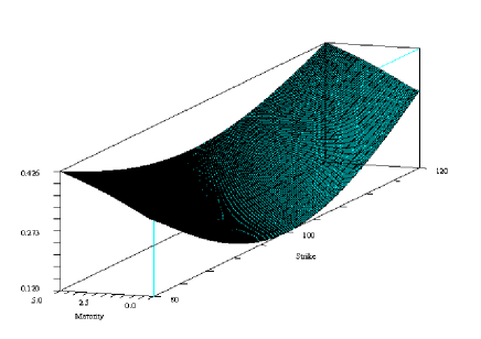
Figure 1: Local volatility function

Basket option

We consider options with payoffs of the form $(\sum_{i=1}^{d}\omega^{i}S_{T}^{i}-K)_{+}$ where $(\omega^{1},\dots,\omega^{d})$ is a vector of algebraic weights. The strike value $K$ can be taken negative to deal with Put like options. With no surprise, we can see on Figure 2 that multilevel estimators always outperform their classical Monte Carlo counterpart. The comparison for very little accurate estimators may be meaningless as it is pretty difficult to reliably measure short execution times and the empirical variance of the estimator is in this case even less accurate than the estimator itself. Note that the points on the extreme right hand side are obtained for multilevel estimators with $L=2$, respectively for Monte Carlo estimators with $256$ samples. For RMSE between $0.1$ and $0.005$, our MLIS estimator is $10$ times faster than the standard ML estimator. When a very high accuracy is required, namely when RMSE is smaller than $0.001$, the MLIS estimator remains between $3$ and $4$ times faster than the standard multilevel estimator, which is already a great achievement since for this level of accuracy, the ML estimator may need several dozens of minutes to yield its result.

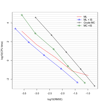
Figure 2: $\sqrt{MSE}$ vs. CPU time for a basket option in the local volatility model with $I=5$, $r=0.05$, $T=1$, $S_{0}=100$, $K=100$, $m=4$.

5.5 Multidimensional Heston model

The multidimensional Heston model can be easily written by specifying on the one hand that each asset follows a 1-D Heston model and on the other hand the correlation structure between the involved Brownian motions. The asset price process $S=(S^{1},\dots,S^{d})$ and the volatility process $\sigma=(\sigma^{1},\dots,\sigma^{d})$ solve

$$dS^{i}_{t} =rS^{i}_{t}dt+\sqrt{\sigma_{t}^{i}}S^{i}_{t}dB^{i}_{t}$$

$$d\sigma^{i}_{t} =\kappa^{i}(a^{i}-\sigma_{t}^{i})dt+\nu^{i}_{t}\sqrt{\sigma^{i}_{t}}(\gamma^{i}dB^{i}_{t}+\sqrt{1-(\gamma^{i})^{2}}d\tilde{B}^{i}_{t})$$

where all the components of $B=(B^{1},\dots,B^{d})$ and $\tilde{B}=(\tilde{B}^{1},\dots,\tilde{B}^{d})$ are real valued Brownian motions. The vectors $\kappa=(\kappa^{1},\dots,\kappa^{d})$ and $a=(a^{1},\dots,a^{d})$ denote respectively the reversion rate and the mean level of each volatility process, while the vector $\nu$ is the volatility of the volatility process. The vector $\bar{\gamma}=(\gamma^{1},\dots,\gamma^{d})$ embodies the correlations between an asset and its volatility process, with $\gamma^{i}\in]-1,1[$ for all $1\leq i\leq d$. The vector valued processes $B$ and $\tilde{B}$ are independent and satisfy

$$d\langle B\rangle_{t}=\Gamma_{S}\,dt\quad\text{and}\quad d\langle\tilde{B}\rangle_{t}=I_{d}\,dt$$

where we assume for our experiments that the covariance matrix $\Gamma_{S}$ has the structure

$$\Gamma_{S}=\begin{pmatrix}1&\rho&\ldots&\rho\\ \rho&1&\ddots&\vdots\\ \vdots&\ddots&\ddots&\rho\\ \rho&\ldots&\rho&1\end{pmatrix}$$ (5.3)

with $\rho\in\left]\frac{-1}{I-1},1\right[$, such that the matrix $\Gamma_{S}$ is positive definite. The processes $B$ and $\tilde{B}$ are Wiener processes with covariance matrices given by $\Gamma_{S}$ and $I_{d}$ respectively.

For the sake of simplicity, we decided not to add any extra correlation between the components of $\tilde{B}$, hence the choice $d\langle\tilde{B}\rangle=I_{d}\,dt$ and we assume in the following that for all the $\gamma^{i}$’s are equal for $1\leq i\leq d$, $\gamma^{i}=\gamma$. The correlations between the volatilities are entirely specified by the correlations between the assets. Even though we do not aim at discussing the correlation structure of the multidimensional Heston model, we believe it is important to make precise the underlying correlation structure in the multidimensional model so that the experiments are easily reproducible.

The model can be equivalently written

$$dS^{i}_{t} =rS^{i}_{t}dt+\sqrt{\sigma_{t}^{i}}S^{i}_{t}dB^{i}_{t}$$

$$d\sigma^{i}_{t} =\kappa^{i}(a^{i}-\sigma_{t}^{i})dt+\nu^{i}_{t}\sqrt{\sigma^{i}_{t}}dW^{i}_{t}$$

where the processes $W$ and $B$ are Wiener processes satisfying

$$d\langle B\rangle_{t}=\Gamma_{S}\,dt;\;d\langle B,W\rangle_{t}=\gamma\Gamma_{S}\,dt;\;d\langle W\rangle_{t}=(\gamma^{2}\Gamma_{S}+(1-\gamma^{2})I_{d})\,dt.$$

The process $(B,W)$ with values in ${\mathbb{R}}^{2d}$ is a Wiener process with covariance matrix

$$\Gamma=\begin{pmatrix}\Gamma_{S}&\gamma\Gamma_{S}\\ \gamma\Gamma_{S}&\gamma^{2}\Gamma_{S}+(1-\gamma^{2})I_{d}\end{pmatrix}.$$

Hence, the pair of processes $(B,W)$ can be easily simulated by applying the Cholesky factorization of $\Gamma$ to a standard Brownian motion with values in ${\mathbb{R}}^{2d}$.

Basket Option

We consider a basket option as in the local volatility model. Figure 3 looks very much the same as in the case of the local volatility model (see Figure 2). The MLIS estimator always outperforms all the ML estimator by a factor of $3$ to $4$. Note that for small RMSE, the computational time can go beyond several hours, hence cutting it down by two or three times represents a real improvement.

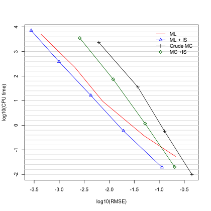
Figure 3: $\sqrt{MSE}$ vs. CPU time for a best of option in the multidimensional Heston model with $I=10$, $r=0.03$, $T=1$, $S_{0}=100$, $K=100$, $\nu=0.01$, $\kappa=2$, $a=0.04$, $\gamma=-0.2$, $\rho=0.3$ and $m=4$.

Best of option

We consider options with payoffs of the form $(\max_{1\leq i\leq d}S_{T}^{i}-K)_{+}$. The payoff of this option does obviously not satisfy the assumptions of Theorem 3.2 as the payoff of the “best of” options is not Hölder with $\alpha\geq 1$. Nonetheless, the multilevel approach beats the standard Monte Carlo technology by far (see Figure 4). Moreover, coupling importance sampling with the multilevel approach improves the accuracy. For a fixed RMSE, we can expect MLIS to be $3$ faster that ML. This example shows the robustness of the method, which performs well whereas the theoretical assumptions are not satisfied.

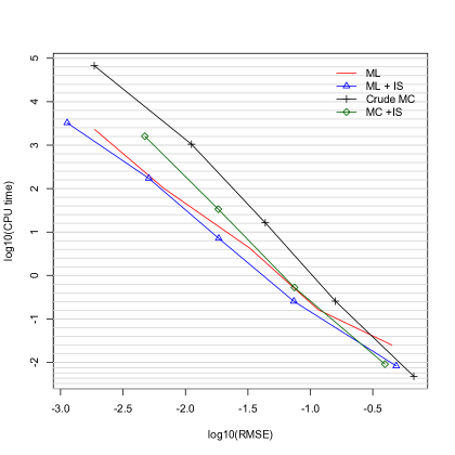
Figure 4: $\sqrt{MSE}$ vs. CPU time for a best of option in the multidimensional Heston model with $I=5$, $r=0.03$, $T=1$, $S_{0}=100$, $K=140$, $\nu=0.25$, $\kappa=2$, $a=0.04$, $\gamma=0.2$, $\rho=0.5$ and $m=4$.

6 Conclusion

We have presented a new estimator making the most of the recent works on multilevel Monte Carlo and on adaptive importance sampling. As expected, this new estimator outperforms the standard multilevel Monte Carlo estimator by a great deal. For a fixed accuracy measured in terms the mean squared error, the MLIS estimator is between $3$ and $10$ times faster that the standard multilevel Monte Carlo estimator. This efficiency of our MLIS approach could still be improved by monitoring the number of samples $N_{\ell}^{\prime}$ to be used to approximate the variance $v_{\ell,N_{\ell}^{\prime}}$ in each level. Actually, we believe that there is no need to compute a too accurate approximation of this variance as a slight decrease in the accuracy of $\hat{\lambda}_{\ell}$ would not lead to a serious deterioration of the accuracy of the MLIS estimator but it could help save a lot of computational time.

Appendix A Auxiliary lemmas

A.1 Central limit theorems for martingale arrays

Theorem A.1 (Central limit theorem for triangular array).

Suppose that $(\Omega,\mathbb{F},{\mathbb{P}})$ is a probability space and that for each $n$, we have a filtration $\mathbb{F}_{n}=(\mathcal{F}_{k}^{n})_{k\geq 0}$, a sequence $k_{n}\longrightarrow\infty\mbox{ as }n\longrightarrow\infty$ and a real vector martingale $Y^{n}=(Y_{k}^{n})_{k\geq 0}$ adapted to $\mathbb{F}_{n}$. We make the following two assumptions.

• 1. There exists a deterministic symmetric positive semi-definite matrix $\varGamma$, such that

     $$\langle Y^{n}\rangle_{k_{n}}=\sum_{k=1}^{k_{n}}\mathbb{E}\left[|Y_{k}^{n}-Y_{k-1}^{n}|^{2}|\mathcal{F}_{k-1}^{n}\right]\overset{\mathbb{P}}{\underset{n\rightarrow\infty}{\longrightarrow}}\varGamma.$$

  2. There exists a real number $a>1$, such that

     $$\sum_{k=1}^{k_{n}}\mathbb{E}\left[|Y_{k}^{n}-Y_{k-1}^{n}|^{2a}|\mathcal{F}_{k-1}^{n}\right]\overset{\mathbb{P}}{\underset{n\rightarrow\infty}{\longrightarrow}}0.$$

Then

$$Y_{k_{n}}^{n}\xrightarrow{\mathcal{L}}\mathcal{N}(0,\varGamma)\quad\mbox{ as }\;n\rightarrow\infty.$$

A.2 Asymptotic behavior of the process $\left(X^{m^{\ell}}-X^{m^{\ell-1}}\right)_{\ell\geq 0}$

In the following we recall some results around the stable convergence. Let $Z_{n}$ be a sequence of random variables with values in a Polish space $E$, all defined on the same probability space $(\Omega,\mathcal{F},{\mathbb{P}})$. Let $(\tilde{\Omega},\tilde{\mathcal{F}},\tilde{\mathbb{P}})$ be an extension of $(\Omega,\mathcal{F},{\mathbb{P}})$, and let $Z$ be an $E$-valued random variable on the extension. We say that $(Z_{n})$ converges in law to $Z$ stably and write $Z_{n}\Longrightarrow^{stably}Z$, if

$$\mathbb{E}(Uh(Z_{n}))\rightarrow\tilde{\mathbb{E}}(Uh(Z))$$

for all $h:E\rightarrow\mathbb{R}$ bounded continuous and all bounded random variable $U$ on $(\Omega,\mathcal{F})$ . According to Section 2 of Jacod [21] and Lemma 2.1 of Jacod and Protter [22], we have the following result

Lemma A.2.

Let $V_{n}$ and $V$ be defined on $(\Omega,\mathcal{F})$ with values in another metric space.

$$\mbox{If }\;\;V_{n}\overset{\mathbb{P}}{\rightarrow}V,\;\;Z_{n}\Longrightarrow^{stably}Z\;\;\;\mbox{then}\;\;\;(V_{n},Z_{n})\Longrightarrow^{stably}(V,X).$$

The following result proved by Ben Alaya and Kebaier [4, Theorem 3] is an improvement of Theorem 3.2 of Jacod and Protter [22], for the setting of Multilevel Euler scheme. More precisely, if $(X^{m^{\ell}}_{t})_{t\geq 0}$ denotes the Euler scheme with time step $m^{\ell}$, with $m,\ell\in{\mathbb{N}}\setminus\{0,1\}$, then we have the following weak convergence in the Skorohod topology.

Theorem A.3.

Assume that $b$ and $\sigma$ are $\mathcal{C}^{1}$ with linear growth then the following result holds.

$$\text{For all}\;m\in\mathbb{N}\setminus\{0,1\},\quad\sqrt{\frac{m^{\ell}}{(m-1)T}}(X^{m^{\ell}}-X^{m^{\ell-1}})\Longrightarrow^{stably}U,\quad\text{ as }\ell\rightarrow\infty,$$

with $(U_{t})_{0\leq t\leq T}$ the $d$-dimensional diffusion process solution to (3.6)

Proposition A.4.

Let $\psi:{\mathbb{R}}^{d}\to{\mathbb{R}}$ be a $C^{1}$ function such that $\psi\in{\cal H}_{\alpha}$, for some $\alpha\geq 1$ and $\nabla\psi$ has at most polynomial growth. For any real valued random variable $Y$ defined on $(\Omega,{\cal F})$ such that ${\mathbb{E}}[\left|Y\right|^{1+\eta}]$, for some $\eta>0$, we have, for any $\delta>0$

$${\mathbb{E}}\left[\left(\frac{m^{\ell}}{(m-1)T}\right)^{\delta/2}\left(\psi(X^{m^{\ell}}_{T})-\psi(X^{m^{\ell-1}}_{T})\right)^{\delta}Y\right]\xrightarrow[\ell\to+\infty]{}{\mathbb{E}}\left[\left(\nabla\psi(X_{T})\cdot U_{T}\right)^{\delta}Y\right].$$

Proof.

The Taylor expansion applied to the real valued function $\psi$ yields

$$\psi(X^{m^{\ell}}_{T})-\psi(X^{m^{\ell-1}}_{T})= \nabla\psi(X_{T})\cdot(X^{m^{\ell}}_{T}-X^{m^{\ell-1}}_{T})$$

$$+(X^{m^{\ell}}_{T}-X_{T})\cdot\varepsilon(X^{m^{\ell}}_{T}-X_{T})-(X^{m^{\ell-1}}_{T}-X_{T})\cdot\varepsilon(X^{m^{\ell-1}}_{T}-X_{T})$$

with $\varepsilon:{\mathbb{R}}^{d}\to{\mathbb{R}}^{d}$ satisfying $\lim_{\left|x\right|\to 0}\varepsilon(x)=0$. From Property ((${\mathcal{H}}$-1)-ii), we easily get

$$\sqrt{\frac{m^{\ell}}{(m-1)T}}\left((X^{m^{\ell}}_{T}-X_{T})\cdot\varepsilon(X^{m^{\ell}}_{T}-X_{T})-(X^{m^{\ell-1}}_{T}-X_{T})\cdot\varepsilon(X^{m^{\ell-1}}_{T}-X_{T})\right)\xrightarrow[\ell\to\infty]{{\mathbb{P}}}0.$$

So, we conclude from Lemma A.2 and Theorem A.3 that

$${\sqrt{\frac{m^{\ell}}{(m-1)T}}}\left(\psi(X^{m^{\ell}}_{T})-\psi(X^{m^{\ell-1}}_{T})\right)\Longrightarrow^{stably}\nabla\psi(X_{T}).U_{T},\;\mbox{ as }\;\ell\rightarrow\infty.$$

Let $\eta>\kappa>0$. From the assumptions on $\psi$ together with Property (${\mathcal{H}}$-1)-ii, we get

$$\sup_{\ell\geq 0}{\mathbb{E}}\left[\left|\left(\frac{m^{\ell}}{(m-1)T}\right)^{\delta/2}\left(\psi(X^{m^{\ell}}_{T})-\psi(X^{m^{\ell-1}}_{T})\right)^{\delta}Y\right|^{1+\kappa}\right]<\infty,$$

which yields the uniform integrability of the family $\left(\left(\frac{m^{\ell}}{(m-1)T}\right)^{\delta/2}\left(\psi(X^{m^{\ell}}_{T})-\psi(X^{m^{\ell-1}}_{T})\right)^{\delta}Y\right)_{\ell}$. The conclusion easily follows. ∎

References

• Arouna [2004] B. Arouna. Adaptative Monte Carlo method, a variance reduction technique. Monte Carlo Methods Appl., 10(1):1–24, 2004. ISSN 0929-9629. doi: 10.1163/156939604323091180. URL http://dx.doi.org/10.1163/156939604323091180.
• Badouraly Kassim et al. [2014] L. Badouraly Kassim, J. Lelong, and I. Loumrhari. Importance sampling for jump processes and applications to finance. Journal of Computational Finance (to appear), 00(00), 2014. http://hal.archives-ouvertes.fr/hal-00842362.
• Ben Alaya and Kebaier [2014] M. Ben Alaya and A. Kebaier. Multilevel Monte Carlo for Asian options and limit theorems. Monte Carlo Methods Appl., 20(3):181–194, 2014. ISSN 0929-9629. doi: 10.1515/mcma-2013-0025. URL http://dx.doi.org/10.1515/mcma-2013-0025.
• Ben Alaya and Kebaier [2015] M. Ben Alaya and A. Kebaier. Central limit theorem for the multilevel monte carlo euler method. Ann. Appl. Probab., 25(1):211–234, 02 2015.
• Ben Alaya et al. [2015] M. Ben Alaya, K. Hajji, and A. Kebaier. Importance sampling and statistical Romberg method. Bernoulli, 21(4):1947–1983, 2015. ISSN 1350-7265. doi: 10.3150/14-BEJ622. URL http://dx.doi.org/10.3150/14-BEJ622.
• Ben Alaya et al. [2016] M. Ben Alaya, K. Hajji, and A. Kebaier. Improved adaptive Multilevel Monte Carlo and applications to finance. 2016. URL http://adsabs.harvard.edu/abs/2016arXiv160302959B.
• Chen and Zhu [1986] H. F. Chen and Y. M. Zhu. Stochastic approximation procedures with randomly varying truncations. Sci. Sinica Ser. A, 29(9):914–926, 1986. ISSN 0253-5831.
• Chen et al. [1988] H. F. Chen, G. Lei, and A. J. Gao. Convergence and robustness of the Robbins-Monro algorithm truncated at randomly varying bounds. Stochastic Process. Appl., 27(2):217–231, 1988. ISSN 0304-4149. doi: 10.1016/0304-4149(87)90039-1. URL http://dx.doi.org/10.1016/0304-4149(87)90039-1.
• Collier et al. [2015] N. Collier, A.-L. Haji-Ali, F. Nobile, E. von Schwerin, and R. Tempone. A continuation multilevel Monte Carlo algorithm. BIT, 55(2):399–432, 2015. ISSN 0006-3835. doi: 10.1007/s10543-014-0511-3. URL http://dx.doi.org/10.1007/s10543-014-0511-3.
• Creutzig et al. [2009] J. Creutzig, S. Dereich, T. Müller-Gronbach, and K. Ritter. Infinite-dimensional quadrature and approximation of distributions. Found. Comput. Math., 9(4):391–429, 2009. ISSN 1615-3375. doi: 10.1007/s10208-008-9029-x. URL http://dx.doi.org/10.1007/s10208-008-9029-x.
• Dereich [2011] S. Dereich. Multilevel Monte Carlo algorithms for Lévy-driven SDEs with Gaussian correction. Ann. Appl. Probab., 21(1):283–311, 2011. ISSN 1050-5164. doi: 10.1214/10-AAP695. URL http://dx.doi.org/10.1214/10-AAP695.
• Duffie and Glynn [1995] D. Duffie and P. Glynn. Efficient Monte Carlo simulation of security prices. Ann. Appl. Probab., 5(4):897–905, 1995.
• Giles [2008a] M. B. Giles. Multilevel Monte Carlo path simulation. Oper. Res., 56(3):607–617, 2008a. ISSN 0030-364X. doi: 10.1287/opre.1070.0496. URL http://dx.doi.org/10.1287/opre.1070.0496.
• Giles [2008b] M. B. Giles. Improved multilevel Monte Carlo convergence using the Milstein scheme. In Monte Carlo and quasi-Monte Carlo methods 2006, pages 343–358. Springer, Berlin, 2008b. doi: 10.1007/978-3-540-74496-2_20. URL http://dx.doi.org/10.1007/978-3-540-74496-2_20.
• Giles and Szpruch [2014] M. B. Giles and L. Szpruch. Antithetic multilevel Monte Carlo estimation for multi-dimensional SDEs without Lévy area simulation. Ann. Appl. Probab., 24(4):1585–1620, 2014. ISSN 1050-5164. doi: 10.1214/13-AAP957. URL http://dx.doi.org/10.1214/13-AAP957.
• Giles et al. [2009] M. B. Giles, D. J. Higham, and X. Mao. Analysing multi-level Monte Carlo for options with non-globally Lipschitz payoff. Finance Stoch., 13(3):403–413, 2009. ISSN 0949-2984. doi: 10.1007/s00780-009-0092-1. URL http://dx.doi.org/10.1007/s00780-009-0092-1.
• Hajji [2014] K. Hajji. Accélération de la méthode de Monte Carlo pour des processus de diffusions et applications en Finance. PhD thesis, Université Paris 13, 2014.
• Heinrich [1998] S. Heinrich. Monte Carlo complexity of global solution of integral equations. J. Complexity, 14(2):151–175, 1998. ISSN 0885-064X. doi: 10.1006/jcom.1998.0471. URL http://dx.doi.org/10.1006/jcom.1998.0471.
• Heinrich [2001] S. Heinrich. Multilevel monte carlo methods. Lecture Notes in Computer Science, Springer-Verlag, 2179(1):58–67, 2001.
• Heinrich and Sindambiwe [1999] S. Heinrich and E. Sindambiwe. Monte carlo complexity of parametric integration. J. Complexity, 15(3):317–341, 1999. ISSN 0885-064X. doi: 10.1006/jcom.1999.0508. URL http://dx.doi.org/10.1006/jcom.1999.0508. Dagstuhl Seminar on Algorithms and Complexity for Continuous Problems (1998).
• Jacod [1997] J. Jacod. On continuous conditional Gaussian martingales and stable convergence in law. In Séminaire de Probabilités, XXXI, volume 1655 of Lecture Notes in Math., pages 232–246. Springer, Berlin, 1997.
• Jacod and Protter [1998] J. Jacod and P. Protter. Asymptotic error distributions for the Euler method for stochastic differential equations. Ann. Probab., 26(1):267–307, 1998. ISSN 0091-1798.
• Jourdain and Lelong [2009] B. Jourdain and J. Lelong. Robust Adaptive Importance Sampling for Normal Random Vectors. Ann. Appl. Probab., 19(5):1687–1718, 2009. doi: 10.1214/09-AAP595. URL http://arxiv.org/pdf/0811.1496v2.
• Kebaier [2005] A. Kebaier. Statistical Romberg extrapolation: a new variance reduction method and applications to option pricing. Ann. Appl. Probab., 15(4):2681–2705, 2005. doi: 10.1214/105051605000000511.
• Lapeyre and Lelong [2011] B. Lapeyre and J. Lelong. A framework for adaptive Monte Carlo procedures. Monte Carlo Methods Appl., 17(1):77–98, 2011. ISSN 0929-9629. doi: 10.1515/MCMA.2011.002. URL http://dx.doi.org/10.1515/MCMA.2011.002.
• Lelong [2008] J. Lelong. Almost sure convergence for randomly truncated stochastic algorithms under verifiable conditions. Statist. Probab. Lett., 78(16):2632–2636, 2008. ISSN 0167-7152. doi: 10.1016/j.spl.2008.02.034. URL http://dx.doi.org/10.1016/j.spl.2008.02.034.
• Lemaire and Pagès [2016 (to appear] V. Lemaire and G. Pagès. Multilevel Richardson-Romberg extrapolation. Bernoulli, 2016 (to appear). URL http://arxiv.org/abs/1401.1177v3.
• Revuz [1997] D. Revuz. Probabilités. Hermann, 1997.
• Rubinstein and Shapiro [1993] R. Y. Rubinstein and A. Shapiro. Discrete event systems. Wiley Series in Probability and Mathematical Statistics: Probability and Mathematical Statistics. John Wiley & Sons Ltd., Chichester, 1993. Sensitivity analysis and stochastic optimization by the score function method.